Abstract
Pseudo-nitzschia spp. blooms are a recurrent problem in many coastal areas globally, imposing some significant threats to the health of humans, ecosystems and the economy. Monitoring programmes have been established, where feasible, to mitigate the impacts caused by Pseudo-nitzschia spp. and other harmful algae blooms. The detection of such blooms from satellite data could really provide timely information on emerging risks but the development of taxa-specific algorithms from available multispectral data is still challenged by coupled optical properties with other taxa and water constituents, availability of ground data and generalisation capabilities of algorithms. Here, we developed a new set of algorithms (PNOI) for the detection and monitoring of Pseudo-nitzschia spp. blooms over the Galician coast (NW Iberian Peninsula) from Sentinel-3 OLCI reflectances using a support vector machine (SVM). Our algorithm was trained and tested with reflectance data from 260 OLCI images and 4607 Pseudo-nitzschia spp. match up data points, of which 2171 were of high quality. The performance of the no bloom/bloom model in the independent test set was robust, showing values of 0.80, 0.72 and 0.79 for the area under the curve (AUC), sensitivity and specificity, respectively. Similar results were obtained by our below detection limit/presence model. We also present different model thresholds based on optimisation of true skill statistic (TSS) and F1-score. PNOI outperforms linear models, while its relationship with in situ chlorophyll-a concentrations is weak, demonstrating a poor correlation with the phytoplankton abundance. We showcase the importance of the PNOI algorithm and OLCI sensor for monitoring the bloom evolution between the weekly ground sampling and during periods of ground data absence, such as due to COVID-19.
1. Introduction
Harmful algae blooms (HABs) in coastal marine systems are an increasingly frequent and intense event that affects the health of humans and the ecosystem and impacts regional economies [1,2]. In recent years, reports on HAB incidences have increased, raising serious concerns [3] of climate change accelerating their frequency [4]. The detection and monitoring of HABs is traditionally based on direct observations, i.e., field samplings at fixed sampling stations [5,6]. However, there is a need for the development of new systems for the detection and monitoring of HABs that will be capable of providing, in real or quasi-real time, synoptic environmental intelligence in order to guide the tactical decisions of industries and authorities. The last decades have witnessed a revolution in Earth observation capabilities for global surface water observation with new missions (e.g., Sentinel) [7]. The increasing availability of satellite data from these missions has profoundly transformed the approaches to monitor and sustainably manage coastal environments [8].
Remote sensing detection (RS) of HABs is usually based on the retrieval of chlorophyll a (Chl-a) as a proxy [9]. Chl-a concentration provides valuable information on phytoplankton biomass but does not discriminate the HAB species from the phytoplankton community. As a result, the HAB-forming species can remain undefined, limiting the direct identification of the specific risks. Species indicator algorithms have been suggested for the direct detection of specific HAB species or taxa from satellite water colour data [10,11,12]. These indicators are founded on the basis that some species have distinct water colour spectra, which can be differentiated by optical sensors. For example, algorithms have been developed to exploit the distinctive features of Karenia brevis in the red part of the electromagnetic spectrum [13,14], and the unique spectral curvatures of taxa such as Coccolithophores [15,16,17] and Trichodesmium [18,19,20].
Spectral band ratios, bio-optical models, data-driven methods and combinations of these have been deployed for the development of species- or taxa-specific algorithms. The authors of [21] summarised the specific challenges associated with the development of HAB detection algorithms from satellite sensors. They highlighted the limitations with regard to the number and position of spectral bands needed to capture the distinctive spectral features of specific species. Moreover, spectral signatures are the result of light interaction with different species, not only the target species, but also with other inorganic and organic components, especially in optically complex waters [22]. In order to deal with these drawbacks and gain a deeper insight into the species’ behaviour, indicators proposed by different authors usually integrate ancillary data [23].
Blondeau-Patissier et al. [24] provided a review of the abovementioned approaches and suggested that hyperspectral sensors can advance the remote detection of species-specific HABs. At the time of writing the manuscript, there were no operational satellite hyperspectral sensors, whereas there is a wealth of historical and current multispectral satellite data at adequate spatial resolutions for monitoring coastal environments. Machine learning methods are appealing in multispectral remote sensing applications since they can have good generalisation ability and problem-solving of complex conditions [25]. A support vector machine (SVM) is a supervised machine learning method of classification or regression based on the use of kernel functions to operate in a feature space with a higher dimension than the input space [26]. SVMs do not make any assumption about data distribution and can model complex and nonlinear data, providing a good generalisation capability [27].
HABs that are attributed to the genus Pseudo-nitzschia plague a number of coastal waters around the world [28] and have significant socioeconomic impacts to the adjacent communities. A number of the species of this genus are known producers of a neurotoxic amino acid, domoic acid (DA), which when accumulated via trophic transfer in the food-web can have deleterious (amnesic shellfish poisoning, ASP) and even fatal effects to several marine organisms and less frequently to humans [29]. Pseudo-nitzschia is common, among others, in areas of coastal upwelling [30]. Recent studies show that occurrence of long-lived, and therefore more threatening, Pseudo-nitzschia blooms off the west coast of the USA [31]. Empirical models [32], regression models and their generalisations have been used for detecting Pseudo-nitzschia spp. at a regional scale from satellite sensors. For example, [33] developed statistical models for Pseudo-nitzschia spp. abundance, particulate DA (pDA) and cellular DA (cDA) in the Santa Barbara channel incorporating ocean colour (MODIS-Aqua and SeaWiFS) and sea surface temperature (AVHRR) data.
This study focuses on the Rias Baixas area in Galicia (NW Spain), where HABs caused by different species, including Pseudo-nitzschia spp., are a frequent and well-documented phenomenon since the 1950s [34]. HABs are monitored by the Technological Institute for the Control of the Marine Environment of Galicia (INTECMAR), which conducts a routine sampling on a weekly basis measuring a set of oceanographic and biological parameters, including the abundance of toxic species and biotoxin levels in molluscs. The authors of [35] found a relationship using regression analysis between pDA and MERIS bands at 510 nm, 560 nm and 620 nm in the area using a rather limited dataset. González Vilas et al. [36] developed an SVM prediction model for Pseudo-nitzschia spp. based on oceanographic parameters. Nevertheless, explicit detection of Pseudo-nitzschia spp. and other species from recent satellite sensors such as Sentinel-3 OLCI data is generally limited, whereas detection models are still challenged by ground data availability and their generalisation capabilities.
Here, we aim to develop a set of new algorithms (PNOI: Pseudo-nitzschia OLCI Indicator) for the detection of Pseudo-nitzschia spp. presence and blooms directly from Sentinel-3 OLCI images based on high performance SVM classifiers and a rich in situ database from the Galician coastal waters. This study also presents a detailed evaluation of the algorithms and a comparison with the linear model.
2. Study Area and Dataset
2.1. The Rias Baixas
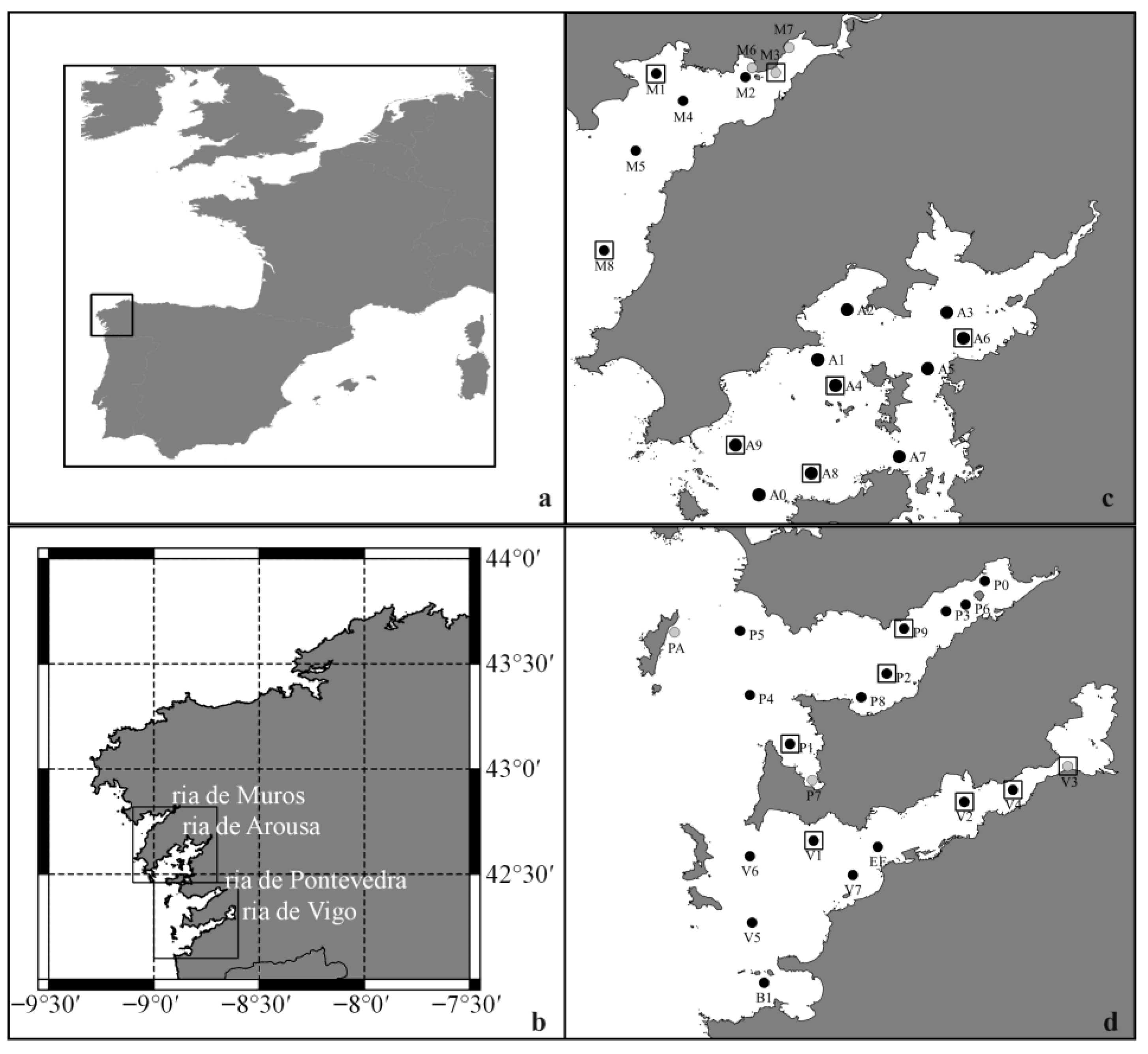
The south-west coast of Galicia (NW Spain) is characterized by the Rias Baixas, i.e., four large V-shaped coastal embayments, from south to north: Vigo, Pontevedra, Arousa and Muros, as shown in Figure 1. Persistent northerly winds cause coastal upwelling events, mainly between May and September, which introduce deep, cold, nutrient-rich waters into the rias and significantly increase their productivity [37]. Due to its high productivity, the area is rich in fish and shellfish resources. There is an intensive mussel culture using floating rafts (bateas) organized in farming polygons, making Galicia the most important producer of aquaculture mussel in Europe and one of the world leaders [38]. In addition to the ecological damage, HABs force the closure of the mussel farming polygons, causing an significant social and economic impact. Although several species of Pseudo-nitzschia spp. have been recorded, only a few have been shown to produce DA [39]. Other taxonomic groups causing HABs in this region are Gynodinium catenatum, Alexandrium minutum and Dynophis spp. [36,40].

Figure 1.
(a) Location of the study area (Galicia, NW Spain). (b) Location of the four Rias Baixas (from north to south: Muros, Arousa, Pontevedra, and Vigo). (c) Location of the sampling stations in the northern rias (Muros and Arousa). (d) Location of the sampling stations in the southern rias (Pontevedra and Vigo). Circles indicate stations with (black) and without (grey) valid Sentinel-3 match-up data. Squares show the stations sampled during the COVID-19 lockdown.
2.2. Sentinel-3 Imagery
A total of 1446 Sentinel-3 images were acquired over the Rias Baixas area between April 2016 and September 2020, of which 989 (68.40%) were totally or partly cloud-free and hence used in this study (Table 1). Sentinel-3 is a European Space Agency (ESA) satellite launched as part of the Copernicus programme. It is mainly an ocean mission based on the heritage of ENVISAT MERIS, which was operational between 2002 and 2012. Its Ocean and Land Colour Instrument (OLCI) covers a swath width of 1270 km, providing the same spatial resolution (300 m) as MERIS, but with more spectral bands (21 instead of 15) ranging from 400 nm to 1020 nm. The mission consists of two satellites (Sentinel-3A and Sentinel-3B), launched in February 2016 and April 2018, respectively. Therefore, revisit time in mid-latitudes have improved from 2–3 days to daily since December 2018, when Sentinel-3B images started to be available [41].

Table 1.
Summary of the Sentinel-3, Pseudo-nitzschia spp. sampling and match-up datasets used in this study for the complete period and study area, and for each year and ria. HQ refers to number of stations with valid high-quality match-ups. In brackets, the surface area of each ria.
2.3. INTECMAR Data
In this study, a database with 7740 records of Pseudo-nitzschia spp. abundance in 465 different days between April 2016 and September 2020 was used (Table 1). INTECMAR conducts a routine monitoring programme consisting of a weekly sampling at 38 sampling stations distributed across the four Rias Baixas (Figure 1). At each station, they measure different water quality parameters (e.g., salinity, temperature) and collect water samples using PVC hoses at three depth ranges (0–5 m, 5–10 m and 10–15 m) and phytoplankton samples using tow nets (10 µm mesh) from surface to 15 m depth. In the laboratory, water samples are analysed in order to determine chlorophyll and inorganic nutrient concentrations [35]. Phytoplankton samples are fixed with formaldehyde 4% and stored under dark and cool conditions. Total abundances (in cells L-1) of different taxonomic groups, including Pseudo-nitzschia spp., are counted using an inverted light microscope at 250× and 400× magnification [42].
3. Methods
3.1. Image Processing and Dataset Generation
Sentinel-3 OLCI images were masked using the pixel identification and classification tool IdePix (release v. 8.0.0), an open processor available in the STEP (Science Toolbox Exploitation Platform) Sentinel-3 toolbox (brockmann-consult.de/portfolio/idepix/). Pixels flagged as invalid, cloud (i.e., cloud_sure, cloud_buffer, cloud_shadow, cirrus_sure, cirrus_ambiguous), land or vegrisk were masked, while the remaining pixels were considered as valid.
Polymer v4.12 was applied for atmospheric correction of the cloud-free Sentinel-3 images. Polymer was developed from an atmospheric correction processor for clear ocean (case-1) waters that is able to deal with sun glint [43] and has shown good results over the study area [44]. It applies a spectral optimization based on a bio-optical model and radiative transfer models to separate atmospheric (including glint) and water reflectances. Output values are provided as fully normalized water-leaving reflectances (https://www.hygeos.com/polymer (accessed on 5 January 2024).
Data from Sentinel-3 images were extracted and linked to the Pseudo-nitzschia spp. database from INTECMAR to create a match-up dataset. A match-up was obtained only if a Sentinel-3 image was available on the same date as the sample collection, and it included the Pseudo-nitzschia spp. abundance and the water-leaving reflectance values from the pixel containing the location of the sampling station. The exact sampling time is unavailable, but samples and images are always acquired in the morning. A match-up was considered as valid if the pixel containing the sampling station was a valid (non-masked) pixel. The number of valid pixels in a 3 × 3 window around the station location was also extracted as a quality flag, ranging from 9 (highest quality) to 1 (lowest quality) [45].
The final match-up dataset included 3008 valid records, of which 2171 were flagged as high-quality (28.05% of the total phytoplankton samples) and were obtained from 260 Sentinel-3 images (55.91% of the total sampling days), as shown in Table 1.
Due to its skewed distribution, Pseudo-nitzschia spp. cell abundance (P-n) was log-transformed (log10P-n) to be used as response variable in the linear regression model. We applied a log10 (1 + P-n) transformation to avoid negative results when P-n was zero.
As SVM models require a categorical output, four categories were established based on the thresholds defined by [36]: below low detection limit (BD) (P-n < 100 cells/L); presence (P) (P-n > 100 cells/L); no bloom (NB) (P-n < 105 cells/L) and bloom (B) (P-n ≥ 105 cells/L). These categories were grouped into three classes when used to analyse the temporal and/or spatial distribution of Pseudo-nitzschia spp.: below low detection limit (BD) (P-n < 100 cells/L); presence—no bloom (P-NB) (100 cells/L ≥ P-n < 105 cells/L) and presence—bloom (P-B) (P-n ≥ 105 cells/L).
3.2. Support Vector Machine Models
We developed an SVM approach for 2-class classification. SVM models were developed using the JAVA version of the LIBSVM library, which applies a sequential minimal optimization-type algorithm [46]. We considered the probability output implemented in LIBSVM, so that probability estimates (between 0 and 1) were computed for each class. Probability models are expected to provide more information, especially when used for building map products such as bloom probability maps. Although different kernels are available, we selected the radial basis function (RFB) because it has been shown to perform slightly better for datasets with a similar size [36,47]. Moreover, it only requires two parameters, reducing the complexity of the model selection process. These are gamma (γ) and cost parameter (C), which control the penalty for misclassification [48].
We developed both a below detection limit/presence (PNOI-BD/P) and a no bloom/bloom (PNOI-NB/B) SVM model using water-leaving reflectance values as input. Instead of a binary output (+1 or −1), we used the probability output for the +1 class, i.e., presence in the PNOI-BD/P model and bloom in the PNOI-NB/B model. Probability values can be converted into a binary result selecting an appropriate threshold and assigning +1 (presence or bloom) if probability is above this threshold or −1 (below detection limit or no bloom) in all other cases.
The complete high-quality (HQ) match-up dataset (2171 records) was divided into two independent and complementary subsets. Both models were developed (e.g., model selection and training) using the training dataset (1628 records, ~75% of total), while the test set (543 records, ~25% of total) was useful for obtaining an independent set of performance measurements. Both subsets were randomly built keeping a similar percentage of both classes and covering the complete temporal (2016–2020) and spatial ranges (across the four rias) observed in the complete dataset.
3.2.1. Scaling and Imbalance Effect
Input variables with larger numeric ranges could have a greater effect on the results [49]. Therefore, input data were linearly scaled to the same range between 0 and 1 using minimum and maximum water-leaving reflectances observed in the complete HQ match-up dataset before training the SVM models [36]. Imbalance in the number of records between both classes observed in the input dataset (mainly for PNOI-NB/B model) can lead to bias towards the majority class causing poorer results. We used weighted SVM to deal with imbalance, i.e., the cost parameter (C) is weighted using a different weight for each class. Hence, a larger weight is applied to the minority class (bloom or below detection limit) in order to improve its accuracy at the cost of a potential increase of misclassification for the majority class (no bloom or presence). In practice, the percentage of records in each class was set as weight of the other class [36]. SVM output values were also scaled between 0 and 1 using minimum/maximum output values in the complete HQ match-up dataset for threshold analysis, model evaluation and map generation.
3.2.2. Model Selection
Since the optimal values for C and γ are unknown a priori for a given problem, we used a simple grid-search approach based on the training dataset to select the optimal parametric configuration. SVM models with different values of C and γ (but keeping the same scaling and weight values) were evaluated using a leave-one-out cross-validation process, i.e., the model is trained N times using N-1 records (N here being the number of elements of the training dataset) and the remaining record is retained for building the confusion matrix and computing the performance measurements. The configuration with the best performance (higher AUC value, see Section 3.2.3) was finally selected.
This approach was implemented in two consecutive phases to save computing time [36]. In the first phase (coarse grid-search), we evaluated 42 SVM models with growing exponential values of C (C = 2−3, 20, 23, 26, 29) and γ (γ = 2−12, 2−9, 2−6, 2−3, 20, 21, 22, 23). In the second phase (fine grid-search), 80 models defined with C and γ values varying around the optimal values found in the first phase (C = 32, γ = 8 for BD/P; C = 8, γ = 8 for NB/B) were assessed. Cross-validation results (including AUC) for all the models included in the coarse and fine grid-searches are shown in the Supplementary Spreadsheets S1 and S2. Once the optimal values of C and γ were found (C = 32.8, γ = 8.4 for BD/P; C = 7.8, γ = 8.4 for NB/B), the final SVM models (PNOI-BD/P and PNOI-NB/B) were trained using the training dataset. These models were used for validation of the independent test dataset and the generation of map products.
3.2.3. Model Evaluation
Performance of SVM models was evaluated using a set of measurements computed from the confusion matrix, a 2 × 2 table reporting the number of true positives, true negatives, false positives and false negatives. Note that our datasets are characterized by a low prevalence, i.e., a low proportion of presence (or blooms) as compared to the total number of measurements. Performance measurements include the sensitivity and the specificity, i.e., the individual accuracies (percentage of records correctly classified) for classes +1 and −1, respectively; the precision, fraction of true positives with respect to the total number of records classified as +1 [50]. Overall accuracy was discarded since it could provide misleading information because of the unequal distribution of classes. Instead, we selected two measurements of overall performance that are less affected by the imbalance of the dataset. These are the true skill statistic (TSS), which combines sensitivity and specificity and are shown to be independent of the prevalence [51], and the F1-score, defined as the harmonic mean of precision and sensitivity. These measurements have been widely used with imbalanced datasets [52]. We worked with two optimal thresholds: one maximizing TSS and other one maximizing F1-score. Note that in PNOI-BD/P, sensitivity is the individual accuracy for the class presence and specificity for below detection limit. In PNOI-NB/B, sensitivity refers to bloom and specificity to no bloom conditions.
As performance measurements derived from the confusion matrix depend on the selected threshold, the Area Under the Receiver Operating Characteristic (ROC) Curve (AUC) was also computed. The ROC curve plots the sensitivity against the false positive rate (1 minus specificity) computed at different probability thresholds. AUC is a measure independent of the threshold and hence it provides useful information when comparing different models. AUC values greater than 0.9 are considered excellent, from 0.8 to 0.9 very good, from 0.7 to 0.8 good, from 0.6 to 0.7 average and lower than 0.6 poor [53].
Figures shown in the work were generated using Matlab R2021b and Microsoft Excel 2019.
4. Results
4.1. SVM Models
SVM models were developed using all the reflectance values as input variables. Considering that some of these variables could introduce noise, models were also trained and validated using combinations of fewer variables. These optimal combinations were selected by applying a variance impact factor (VIF) collinearity analysis to remove autocorrelated variables (with VIF < 5) [54], and/or filtering variables that do not show significant differences between abundance classes (see Section 4.2). However, results were worse than the obtained ones using all the reflectances and hence are not shown in this work.
Results from both PNOI-BD/P and PNOI-NB/B models are summarized in Table 2. Results from the leave-one-out cross-validation shown in this table were obtained using the optimal parametric configuration selected as the one with highest AUC value in the grid-search approach, while results from training and test sets were obtained using the final models derived from applying the selected optimal configuration to the training dataset (see Section 3.2.2). Note that metrics from the test set provide an independent evaluation of their performance. All the measurements based on the confusion matrix (all except AUC) shown in Table 2 (see Section 3.2.3) were computed using the threshold maximizing the TSS.
Table 2.
Performance measures computed from leave-one-out cross-validation (LOU CV) process and from the training and test sets using PNOI-BD/P and PNOI-NB/B models. Results are based on the optimal parametric configuration. Parameters (except for AUC) were computed using the optimal threshold selected by maximizing TSS. #NB, number of no bloom; #B, number of bloom; #BD, number of below detection limit; #P, number of presence; Sens., sensitivity; Spec., specificity; Prec., precision; TSS, True Skill Statistic; F1, F1-score and AUC are shown in the table.
According to the results from the leave-one-out cross-validation, both PNOI-BD/P and PNOI-NB/B show good (over 0.70) AUC values [53] and the same TSS value with a good balance between sensitivity and specificity. However, precision (and hence F1-score) values are strongly affected by the unequal distribution of both classes. Although PNOI-NB/B shows a slightly higher specificity (0.72 against 0.71) and hence lower rate of false positives, the low prevalence, i.e., the higher number of no bloom (1393) as compared to the number of bloom (235), leads to a higher absolute number of false positives in contrast to the number of true positives resulting in poorer precision (0.30 against 0.79).
As expected, results from the training set are better than the ones obtained from the leave-one-out cross-validation process, with AUC values over 0.90 for both models. PNOI-NB/B outperforms PNOI-BD/P in terms of sensitivity and specificity, with higher AUC and TSS values, although it shows a lower precision (and F1-score) because of the imbalance in the training set.
Results from the independent test set, which is not included in the training process, are comparable to the ones derived from the cross-validation, evidencing the robustness and good generalisation capability of the models. In the case of PNOI-BD/P, it shows a lower AUC and a worse balance between sensitivity and specificity, but results are similar in terms of sensitivity and precision. Regarding PNOI-NB/B, results from the test set are even better in terms of AUC, specificity, precision and F1-score.
4.2. Comparison with the Linear Model
A linear regression model based on the complete HQ match-up dataset (N = 2171), using all the water-leaving reflectances as input and Pseudo-nitzschia spp. abundances (log10P-n) as output was developed as a standard method to compare with SVM models. We found a significant correlation between the observed and predicted Pseudo-nitzschia spp. abundance (r = 0.42, p < 0.01, RMSE (root mean squared error) = 2.03).
Table 3 shows the classification results obtained from the complete dataset using PNOI-BD/P and PNOI-P-NB/B and this linear model, as well as the classification results in terms of bloom detection for the consecutive application of PNOI-BD/P and PNOI-NB/B (meaning that PNOI-NB/B is only applied to records classified as presence). For the SVM models, performance measurements based on the confusion matrix (all except for AUC) were computed using two thresholds: one maximizing the F1-score and other one maximizing the TSS. For the linear model, classification results were obtained by applying the thresholds defined for discriminating abundance categories (log10P-n = 3 for BD/P, log10P-n = 5 for NB/B) to the predicted Pseudo-nitzschia spp. abundances.
Table 3.
Performance measures computed from the complete dataset for PNOI-NB/B, PNOI-BD/P and linear model, and bloom classification results for the consecutive application of PNOI-BD/P and PNOI-NB/B. Parameters (except for AUC) for PNOI models were computed using two thresholds selected by maximizing TSS and F1-score (F1). #NB, number of no bloom; #B, number of bloom; #BD, number of below detection limit; #P, number of presence; Sens., sensitivity; Spec., specificity; Prec., precision; TSS, True Skill Statistic; F1-score and AUC, are shown in the table.
5. Discussion
5.1. Spatial and Temporal Distribution of Pseudo-nitzschia spp. Abundance
Table 4 summarizes the spatial distribution of Pseudo-nitzschia spp. abundance across the four rias in the INTECMAR and high-quality (HQ) match-up datasets. There is a higher sampling effort in Pontevedra, despite not being the largest ria. Pontevedra seems to be the ria most affected by HABs (not only due to Pseudo-nitzschia spp.). In the remaining rias, the sampling effort is related to their size.
Table 4.
Average and standard deviation of Pseudo-nitzschia spp. abundance and distribution of the three abundance categories (BD: below detection limit, P-NB: presence—no bloom and P-B: presence—bloom) are shown for the complete study area and for each ria. Top row shows the values in INTECMAR dataset, while bottom row the ones in the high-quality match-up dataset.
The match-up dataset contains approximately 60% of INTECMAR data (4607 of 7740), showing a coverage around 60% for each individual ria (Table 1). In the HQ match-up dataset (as defined above), this is reduced to 28.05% (2171 of 7740), with an unequal distribution across the rias: 40.94% in Arousa, 19.31% in Pontevedra and values around 25% in Vigo and Muros (Table 4). The observed differences are most likely caused by varying cloud cover across the study area. Six stations (one in Vigo, two in Pontevedra and three in Muros) were not included in the match-up dataset due to their proximity to the coastline (Figure 1c,d). Moreover, only a limited set of stations (three in Muros and Pontevedra, four in Vigo and Arousa) was sampled during the COVID-19 lockdown from 17 March to 18 May 2020 (Figure 1c,d). Despite the differences in coverage, the HQ match-up dataset is representative of the INTECMAR database showing similar percentages of the three abundance classes in all rias.
In situ observations of Pseudo-nitzschia spp. abundances between pairs of rias were compared using pairwise Mann–Whitney tests. Results revealed that only Muros shows a significantly (p < 0.01) higher abundance (2.98 log10P-n(cells/L)) when compared to other rias. Muros is hence the ria most affected by Pseudo-nitzschia spp., with the highest percentage of samples classified as bloom (17.62%) and the lowest percentage of below detection limit samples (34.20%). In the remaining rias, the percentage of bloom varies from 13.80% (Vigo) to 9.57% (Arousa) (Table 4).
In the HQ match-up dataset, the spatial distribution patterns are similar, with Muros representing the ria recording the highest percentage of blooms (18.82%). In the remaining rias, bloom incidence varies from 12.13% in Arousa to values around 15% in Vigo and Pontevedra (Table 4).
Sampling effort by year is summarized in Table 1. Since 2019, the availability of Sentinel-3B data has improved the temporal coverage (daily temporal resolution). This is also reflected in the HQ match-up database, with 40% of the total number of samples against lower than 20% in 2017 and 2018.
Table 5 shows the differences in Pseudo-nitzschia spp. abundance across the years. Abundances in 2017 (3.12 log10P-n[cells/L]) are significantly higher (p < 0.01) than in other years. Data from 2016 and 2018 show a similar pattern with a percentage of bloom around 15% and abundances significantly higher (p < 0.01) when compared to 2019 and 2020. The HQ match-up dataset follows the temporal patterns observed in the INTECMAR database (Table 5), although showing a lower percentage of below detection limit records and a slightly higher incidence of blooms (except for 2017).
Table 5.
Average and standard deviation of Pseudo-nitzschia spp. abundance and distribution of the three abundance categories (BD: below detection limit, P-NB: no bloom and P-B: bloom) are shown for each year using the INTECMAR (top row) and high-quality match-up datasets (bottom row) of Pseudo-nitzschia spp.
Figure 2 summarizes the temporal distribution of the sampling coverage, showing the number of valid HQ match-ups by month and year, as well as the overall coverage. Data for 2020 were only available until September. Overall coverage was defined as the percentage of valid HQ match-ups per month. The maximum overall coverage was reached in July. Figure 2 demonstrates Sentinel-3 observational capabilities for capturing the seasonal variability in the area and representativeness of the match-up dataset for the development of Pseudo-nitzschia spp. algorithms.
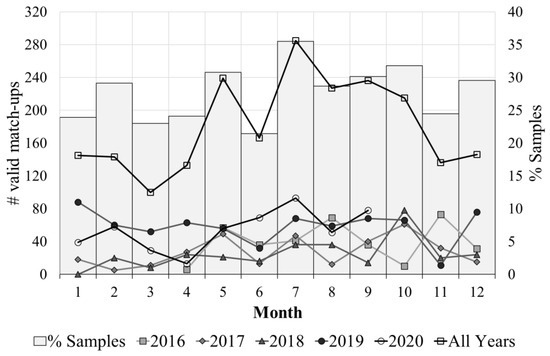
Figure 2.
Lines show the number of valid match-ups by month. Bars show the sampling coverage defined as the percentage of total samples collected by INTECAR per month that were extracted as a valid match-ups.
5.2. Relationships between Pseudo-nitzschia spp. Abundance and Sentinel-3 Data
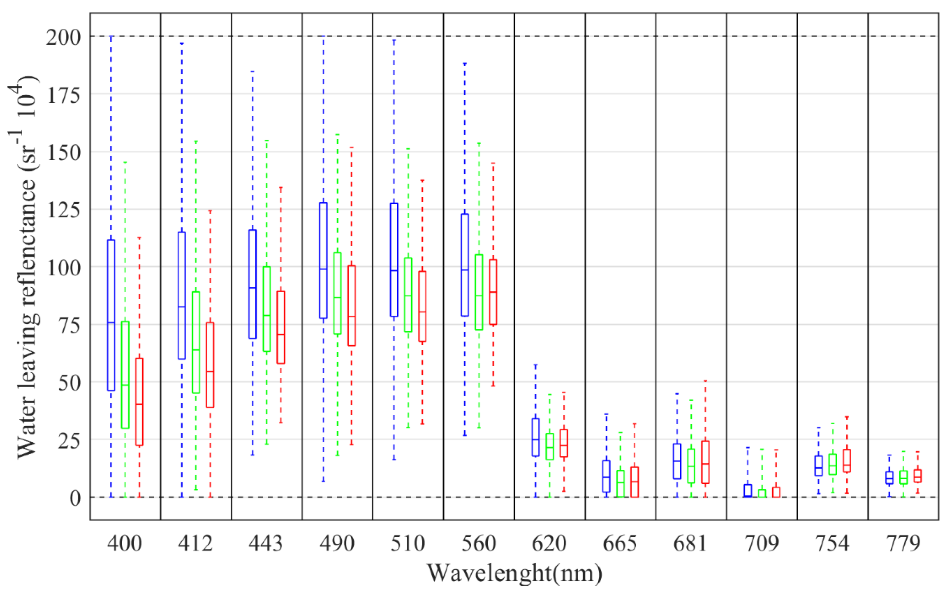
Figure 3 summarizes the statistics computed from each band and Pseudo-nitzschia spp. abundance category using water-leaving reflectance data computed using Polymer 4.12 starting from the HQ match-up dataset. Differences in mean values among the three categories are especially evident in the blue part of the spectrum, while these are smaller towards the red part of the spectrum.
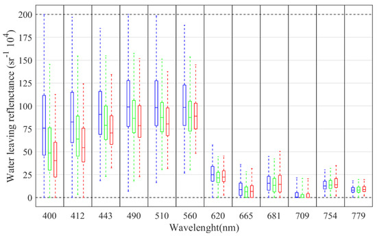
Figure 3.
Summary statistics for each band and abundance class (blue: below detection limit; green: presence—no bloom; and red: presence—bloom) derived from the high-quality match-up dataset using water-leaving reflectance values (multiplied by 104) computed using Polymer v. 4.12. On each box, the central mark shows the median while the bottom and top edges indicate the 25th and 75th percentiles, respectively. Whiskers extend to the minimum and maximum values.
Results from Kruskal–Wallis tests revealed significant differences among the three abundances categories for all the reflectances (p < 0.05 for 779 nm, p < 0.01 for the remaining bands). Significant differences were also observed using Mann–Whitney tests (p < 0.01) between below detection limit and presence classes for all the bands expect for 779 nm. Regarding no bloom and bloom classes, Mann–Whitney tests show significant differences (p < 0.01) for all the bands except for 620 nm, 665 nm and 681 nm.
There is limited information on the spectral signatures of Pseudo-nitzschia spp. in the literature. Our results show that Pseudo-nitzschia spp. blooms are mainly characterized by lower reflectances in the blue region (between 400 nm and 510 nm), where coloured dissolved organic matter and detritus have also a strong absorption effect [55,56]. Anderson et al. [33] suggest that UV-absorption by accessory Pseudo-nitzschia pigments could also contribute to increased absorption in the blue part of the spectrum. The latter study found a negative correlation between Pseudo-nitzschia spp. abundance and the ratio Rrs (412/555), which is also observed in our dataset (with Rw(412/560), r = −0.17). We also detected a negative correlation between Pseudo-nitzschia spp. abundance and the ratio Rw(510/560), indicating that HAB events could be associated with high Chl-a biomass patches. Chlorophyll is common to almost all the phytoplankton taxonomic groups and its concentration is not expected to depend only on Pseudo-nitzschia spp. abundance.
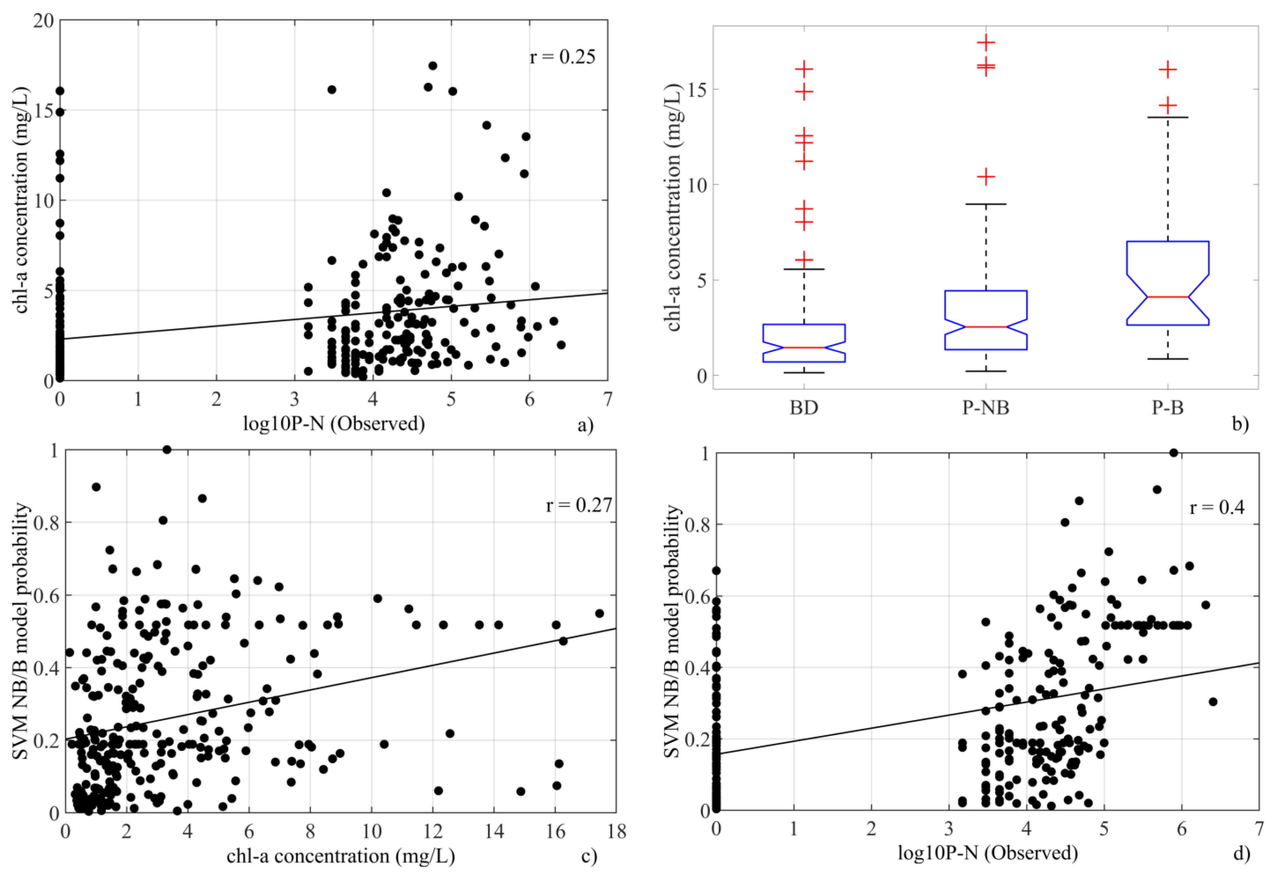
In this study, the in situ Chl-a concentrations were weakly correlated with Pseudo-nitzschia spp. abundances (r = 0.25, Figure 4a). However, there are significant differences among the three abundance categories according to the Kruskal–Wallis test results (Figure 4b). While below detection limit (BD) records are related to situations with low Chl-a (and probably low phytoplankton abundance), presence—bloom (P-B) records show significantly higher concentrations.
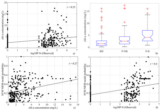
Figure 4.
(a) Relationship between Pseudo-nitzschia spp. abundances (log10P-n) and in situ Chl-a concentrations. (b) Graphical comparison of in situ Chl-a concentrations among Pseudo-nitzschia spp. abundance categories (BD: below detection limit, P-NB, presence—no bloom and P-B: presence—bloom). (c) Relation between in situ Chl-a concentrations and bloom probabilities from PNOI-NB/B. (d) Relation between log10P-n and bloom probabilities from PNOI-NB/B.
Despite the relationships observed with Pseudo-nitzschia spp. abundance, model results cannot be explained only by the Chl-a concentration. In fact, bloom probability computed using PNOI-NB/B is weakly correlated with in situ Chl-a (Figure 4c, r = 0.27) but shows a better correlation with log10P-n (Figure 4d, r = 0.40).
5.3. Performance of Models and Threshold Analysis
PNOI models outperform the linear model (Table 3) in terms of both presence and bloom detection. The two methods are based on different foundations, i.e., linear models work as approximation functions while SVM are specifically designed for classification problems, as well as their ability to deal with more complex and nonlinear patterns. Note also that PNOI models were developed using only the training dataset (75% of the records).
Using the linear model, we found a significant correlation between the observed and predicted Pseudo-nitzschia spp. abundance (r = 0.42, p < 0.01; RMSE = 2.03), as well as between Pseudo-nitzschia spp. abundances and output probabilities from PNOI-BD/P (r = 0.64, p < 0.01) or PNOI-NB/B (r = 0.40, p < 0.01).
The results of our linear model (adjusted R2 = 0.17) are worse than those obtained by [31]. They found stronger correlations in the development of their best remote sensing model (true skill (equivalent to an adjusted R2) = 0.63) and also in the independent validation set based on SeaWiffs data (R2 = 0.32, p = 0.03). However, in terms of classification, PNOI-NB/B improved the results attained by [31], using their remote sensing model, which correctly classifies 53% of bloom and 96% of no bloom observations. Note that their models also include Chl-a concentrations.
Results from PNOI-BD/P and PNOI-NB/B were compared using two thresholds: one maximizing TSS, which implies a better balance between sensitivity and specificity, and the other one maximizing the F1-score, which is achieved with a higher accuracy of the majority class. Results using both thresholds are different because of the imbalance in the datasets (Table 3).
In case of PNOI-BD/P, the highest F1-score (0.86) is achieved with a middle threshold (0.504) resulting in high sensitivity (0.91), i.e., a high individual accuracy in the majority presence class, but at the cost of a lower specificity (0.64). Increasing the threshold, more records are identified as below detection limit so that specificity increases while sensitivity decreases. TSS is maximized with a threshold of 0.640 (TSS = 0.58), with values of sensitivity and specificity around 0.80 and with a higher precision (0.85).
Regarding PNOI-NB/B, the pattern is inverse since no bloom is the majority class: the highest F1-score is obtained with maximum specificity (0.93) and lower sensitivity (0.79) at a middle threshold (0.512). As the threshold decreases, more records are classified as bloom, increasing the sensitivity at the cost of a lower specificity. The best balance is achieved with a threshold of 0.430 (TSS = 0.75), with values of sensitivity and specificity of 0.87.
Note that the F1-score depends on the balance between both classes. Using PNOI-NB/B, with a low prevalence in the input dataset (less bloom than no bloom), the highest F1-score is achieved with the highest precision. However, with PNOI-BD/P, the positive condition is predominant (more presence than below detection limit) and the highest F1-score is obtained with the highest sensitivity.
Overall, PNOI-NB/B outperforms PNOI-BD/P as it shows higher AUC values (a measurement independent of the threshold), and TSS (a measurement that is shown to be independent of the prevalence). The lower precision and F1-score values are related to the extremely low prevalence (only 15% of records are blooms) observed in the input dataset, so that the absolute number of false positives (130 with a specificity of 0.93) is higher than the number of true positives (247 with a sensitivity of 0.79).
Bloom detection capability was also evaluated with a two-step procedure using first PNOI-BD/P and then applying PNOI-NB/B only to records classified as presence. According to the measurements shown in Table 3, the previous application of PNOI-BD/P to exclude below detection limit records does not imply a significant improvement: results are similar when the F1-score threshold is used with PNOI-BD/P and worse when the TSS threshold is applied.
Classification results of the linear model were better in terms of presence detection because there is a more equal distribution of classes (BD: 38.3%; P: 61.7%), so that this model is able to correctly identify 56% of the observations as presence (sensitivity = 0.56, see Table 3). However, in terms of bloom detection, the linear model shows a strong bias towards the majority class (NB: 85.6%; B: 14.4%), identifying 99% (specificity = 0.99, see Table 3) of no bloom situations but at the cost of an extremely low sensitivity (only correctly identify 1% of blooms). In both cases, results from linear models were worse than those obtained using PNOI considering all the metrics (Table 3).
5.4. Model Evaluation and Filling Observational Gaps of Pseudo-nitzschia spp. Evolution
Given that the monitoring data are collected at each station on a weekly basis by INTECMAR, we used Sentinel-3 OLCI images acquired between the ground observations to evaluate the evolution of the Pseudo-nitzschia spp. abundance and complement, to some extent, the information provided by the monitoring program. We obtained the distribution of the three abundance categories (BD, P-NB and P-B) at stations between the dates of ground observations. PNOI-BD/P was first applied to discriminate between below detection limit and presence, and then PNOI-NB/B was applied to stations classified as presence to distinguish between no bloom and bloom. In both cases, discriminations were based on the threshold-maximizing TSS (0.640 for PNOI-BD/P model, 0.430 for PNOI-NB/B, see Table 3). Figure 5 summarizes the results, as well as the observed category on the initial and final sampling dates and the number of weeks with each specific change according to the INTECMAR database.
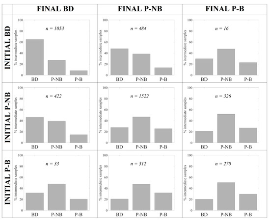
Figure 5.
Distribution of the three abundance categories (BD, P-NB and P-B) at stations derived from Sentinel-3 OLCI images acquired between two in situ sampling dates using PNOI-BD/P and PNOI-NB/B models. The observed category on the initial and final sampling dates are shown for each row and column, respectively, while n indicates the total number of weekly observations with that specific change.
The abundance category (BD, P-NB and P-B) does not change in 64.11% of the weekly observations, summing 7381 observations in images acquired between the initial and final sampling dates. In more than half of these observations (51.47%), the inter-weekly Pseudo-nitzschia spp. abundance derived from PNOI remained in the same category. This was more apparent with below detection limit cases (near 65%), meaning that in 65% of the cases where ground observations in two consecutive weeks were classified as below detection limit, the abundance of Pseudo-nitzschia spp. remained below detection limit within these two observations.
In 34.79% of the weeks, Pseudo-nitzschia spp. abundance showed a moderate increase (BD to P-NB, P-NB to P-B) or decrease (P-B to P-NB, P-NB to BD) between two observations. In these observations, blooms are captured from the inter-weekly Sentinel-3 images before being identified by the monitoring programme in 26.8% of stations with changes from P-NB to P-B, while the end of the bloom is observed in nearly half of stations (46.26% of P-NB with changes from P-B to P-NB).
Abrupt changes at stations from below detection limit to bloom and vice versa are less frequent (only 1.10% of the weeks, 1.47% of the observations in images). OLCI images acquired between the weekly observations were able to predict blooms in advance in 22.81% of the stations with changes from BD to P-B, and 31.62% of the inverse situations from P-NB to BD.
Overall, 63.52% of stations derived from Sentinel-3 inter-weekly images showed coherent Pseudo-nitzschia spp. abundance categories compared to the INTECMAR database. Considering only stations without a change in the abundance category, this accuracy is reduced to 51.47%. When both images on sampling and intermediate dates were considered, overall accuracy was 64.51%. Values are similar in the four rias, varying from 62.87% in Pontevedra to 66.18% in Vigo. Greater variations are observed among individual stations (from 48.39% to 70.83%), with lower accuracies in the stations which are more affected by blooms events.
A ria seems to usually show four types of situations on a specific date in terms of Pseudo-nitzschia spp. distribution: absolute absence (21.73%), presence without blooms (55.46%), widespread bloom (3.70%) or mixed situations (19.10%) which some stations measured as presence and other ones as bloom with abundances around the threshold (105 cells/L). Around 19.1% of false positives (no bloom classified as bloom) correspond with mixed situations, i.e., blooms were observed at other stations on the same date and ria, while 55.5% correspond with presence without bloom situations. Only 8.26% (10 false positives) were detected in situations with an absolute absence of Pseudo-nitzschia spp. on that date and ria. Regarding the false negatives (bloom classified as no bloom), 88.9% were recorded in mixed situations with presence observations at other stations on the same date and ria. Note that misclassifications in presence and mixed situations (91.1% of all the errors) could be explained by other factors related to the variability of Pseudo-nitzschia spp. in a highly dynamic environment. For instance, samples are collected in a specific location, while Sentinel-3 pixels cover a 300 m2 area, and at a different time than the satellite overpass (time difference is usually lower that 2–3 h). Moreover, there is some uncertainty in the discrimination between no bloom and bloom in the laboratory with abundances around the threshold value.
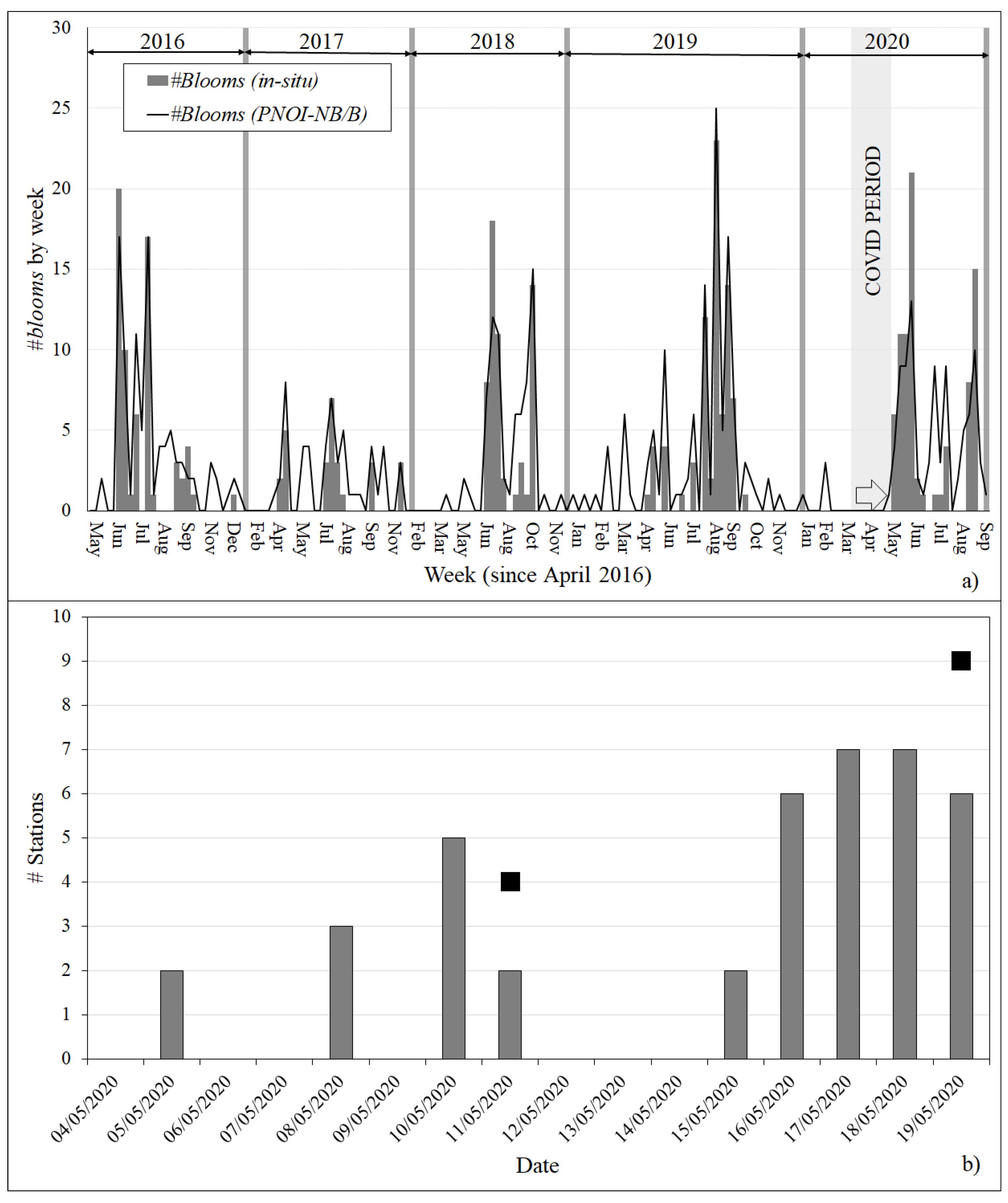
Figure 6a shows the temporal evolution of the number of blooms observed in the INTECMAR database every week since April 2016, in comparison with the number of blooms detected on the same dates at INTECMAR stations by applying PNOI-NB/B to the available Sentinel-3 images. Overall, the model is able to follow a similar pattern, correctly discriminating weeks affected by high abundances (i.e., with more than five stations with an observed bloom) from other ones without blooms. The number of false positives observed in weeks without episodes is usually low (1–2) as compared to the total number of stations, showing that images do not provide misleading information (i.e., a high number of blooms during “no bloom” weeks) despite some timing errors. Data are available in the Supplementary Spreadsheets S3, where Figure S1 shows the error expressed as the difference in the number of weeks affected by bloom observed and predicted using PNOI-NB/B.
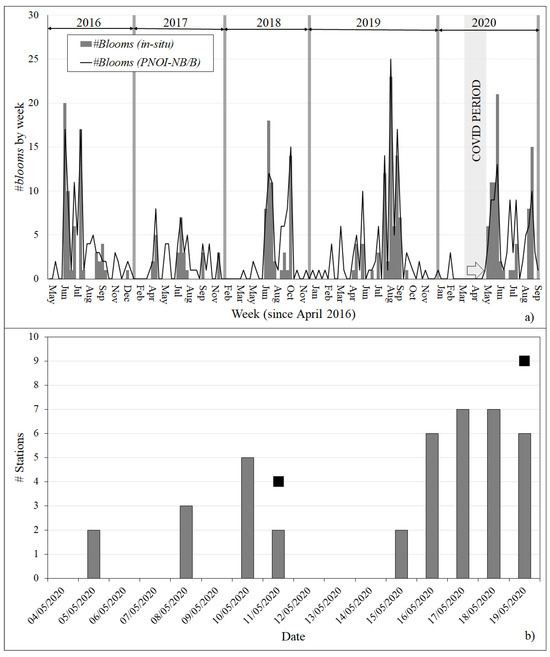
Figure 6.
(a) Number of Pseudo-nitzschia spp. blooms observed in the INTECMAR in situ database and detected in the Sentinel-3 images applying PNOI-NB/B at the same stations by week since April 2016, using only images on sampling dates. (b) Number of stations in ria de Vigo classified as presence applying PNOI-BD/P to Sentinel-3 images between 4 and 19 May 2020. Black squares indicate the number of stations sampled by INTECMAR, all of them categorised as presence.
Satellite information is extremely useful in cases where ground data are limited or unavailable. During eight weeks in 2020 (from 17 March to 18 May, Figure 6a), INTECMAR collected a limited number of samples at fewer stations (four in Vigo and Arousa, three in Pontevedra and Muros, Figure 1c,d), because of the COVID-19 lockdown in Spain. During the first seven weeks, most of the stations were monitored as below detection limit in the INTECMAR in situ database. On 11 May, during the last lockdown week, there was a change in the tendency in rias de Vigo and Pontevedra, with the seven sampled stations categorized as presence and a maximum of 77,220 cells/L. This tendency was confirmed in the first week after the lockdown with the in situ samplings conducted on 18 and 19 May 2020, characterized by a generalized presence across the four rias (37 of 38 stations), an extended bloom in ria de Pontevedra (at 8 of 11 stations) and other bloom at 1 station in ria de Muros. This episode affecting the four rias continued for four to five weeks until mid-June (Figure 6a).
Model results from Sentinel-3 images available during the last two lockdown weeks (from 4 May to 17 May) were able to anticipate this increasing tendency in Pseudo-nitzschia spp. abundance. Figure 6b shows the example in the ria de Vigo, where samples were not collected in the week starting on the 4 May because of bad weather conditions. Stations classified as presence using PNOI-BD/P were first detected on 5 May, and then in different images on both sampling (11 May and 19 May) and intermediate dates. A similar pattern with a generalized presence was observed in the other three rias using PNOI-BD/P. Moreover, some blooms were detected using PNOI-NB/B. For instance, PNOI-NB/B detected blooms at four stations between the 16th and 18th. These were then confirmed by the in situ sampling conducted on 19 May.
5.5. Pseudo-nitzschia spp. Maps
PNOI models can be used for the generation of maps from Sentinel-3 images, including presence and bloom probability maps as well as binary BD/P or NB/B maps. Maps are helpful for the detection of potential blooms of Pseudo-nitzschia spp. in the Rias Baixas area and to complement the information of the INTECMAR monitoring program. Usefulness of these maps depends on their capability to detect the spatial and temporal distribution patterns of Pseudo-nitzschia spp. abundance and blooms observed in the monitoring program. In this work, the high-quality match-up dataset derived from Sentinel-3 images has proven to be representative of the complete INTECMAR dataset, showing similar distribution patterns across the four rias (Table 4).
Sentinel-3 also provides an excellent temporal resolution because these images are available on a daily basis since December 2019 with a two-satellite configuration (Sentinel-3A and Sentinel-3B). However, one of the main limitations of using colour images in an operational way is the availability of cloud-free scenes. In this study, approximately 70% of the total images were totally or partly cloud-free over the Rias Baixas area and hence available for obtaining maps (Table 1). Moreover, more cloud-free images are expected to be available during the period with a higher percentage of blooms (between May and October, see Figure 3). Note that a potential limitation could be the local morning fogs observed during the summer months, which could explain the lower sampling coverage in June (Figure 2).
Figure 7 shows some examples of bloom probability maps derived from Sentinel-3 images using PNOI-NB/B reflecting the temporal and spatial patterns observed in the INTECMAR database. Indeed, the model is able to distinguish situations where blooms affected all four rias (Figure 7c) and when Pseudo-nitzschia spp. was hardly present in the area (Figure 7a). Maps are also useful for analysing the relative spatial distribution of abundance and blooms, with differences among rias and even within the same ria (Figure 7c). In terms of temporal evolution, maps are also able to detect changes in Pseudo-nitzschia spp. abundance. For instance, the development of a bloom in the southern rias between 12 June 2019 (Figure 7a) and 16 June 2019 (Figure 7b) is observed.
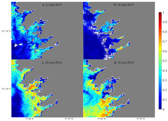
Figure 7.
Bloom probability maps derived from Sentinel-3 images using PNOI-NB/B: (a) 12 June 2019; (b) 16 June 2019; (c) 20 June 2016; and (d) 19 June 2018.
6. Conclusions
Results from this work show the potential of Sentinel-3 images and PNOI models for the monitoring of Pseudo-nitzschia spp. blooms and to provide complementary information to the in situ monitoring programme. Use of our developed approach could be even more important during situations in which field monitoring is not available (e.g., ship breakdown, sampling mistakes) or limited. For instance, during the COVID-19 restrictions between March and May 2020, only a limited number of stations was sampled. Situations of extreme weather conditions prevent both in situ samples and cloud-free Sentinel-3 images from being obtained, but fortunately these situations are not common (usually two to three weeks per year in winter) and are not usually associated with HABs.
The main limitation of our approach is that PNOI does not discriminate the different Pseudo-nitzschia species. Discrimination down to species level is hard even in in situ samples since it often requires scanning electron microscopy. Since not all the species are toxic, blooms are not necessarily toxigenic. In fact, only P. australis has been shown to produce domoic acid in the region [33,37]. With this limitation in mind, PNOI could be improved by using it as the basis for the development of a higher-level product that could provide mussel producers with more useful information. The next steps will include the following: 1) identification of toxigenic blooms by associating Pseudo-nitzschia spp. abundance data with domoic acid concentrations and/or closures of mussel production polygons because of ASP events; and 2) integration with auxiliary data, such as temperature, salinity or upwelling indices, in order to reduce the false alarm rate and discriminate between toxigenic and non-toxigenic blooms.
Toxic blooms of Pseudo-nitzschia spp. are a problem in other coastal areas of the world and results from this work show that remote sensing could be a useful tool for detection and monitoring. At the time of writing this manuscript, PNOI models have been evaluated by the Regulatory Council of Mussel from Galicia in the framework of the CoastObs project. Specifically, bloom probability maps based on Sentinel-3 images were produced operationally and made available through a dedicated Lizard web portal. In other areas, S-3 EUROHAB (https://www.s3eurohab.eu/ (accessed on 5 January 2024)) projects have also explored the potential of Sentinel-3 images for detecting eutrophication and HABs, including Pseudo-nitzschia spp., in the French–English Channel [57].
Supplementary Materials
The following supporting information can be downloaded at: https://www.mdpi.com/article/10.3390/rs16020298/s1. Spreadsheet S1: Cross-validation results (including AUC) for all the models below detection limit/presence (BD/P) included in the coarse and fine grid-search. Spreadsheet S2: Cross-validation results (including AUC) for all the models no bloom/bloom (NB/B) included in the coarse and fine grid-search. Spreadsheet S3: Number of Pseudo-nitzschia spp. blooms observed in the INTECMAR in situ database and detected in the Sentinel-3 images applying PNOI-NB/B at the same stations by week since April 2016, using only images on sampling dates. Figure S1: Difference in the number of weeks affected by bloom observed and predicted using PNOI-NB/B since April 2016.
Author Contributions
Conceptualization, L.G.V., E.S. and J.M.T.P.; methodology, L.G.V. and E.S.; analysis, L.G.V., Y.P. and E.S.; writing—original draft preparation, L.G.V., J.M.T.P. and E.S.; writing—review and editing, L.G.V., E.S. and J.M.T.P.; visualization, L.G.V.; supervision, L.G.V., E.S. and J.M.T.P.; project administration, J.M.T.P.; funding acquisition, E.S. and J.M.T.P. All authors have read and agreed to the published version of the manuscript.
Funding
This study was funded by the European Union’s Horizon 2020 research and innovation programme (grant agreement No 776348).
Data Availability Statement
Maps obtained using the algorithm presented in this study are available from the CoastObs portal (https://coastobs.lizard.net). More information is available in the Zenodo dataset: Lazaros Spaias, Mariana Mata Lara, Evangelos Spyrakos, Federica Braga, Vittorio E. Brando, Laura Zoffoli, Pierre Gernez, Anne-Laure Barillé, Tony van der Hiele, Luis González Vilas, Jesus M. Torres, Annelies Hommersom, Steef Peters, Caitlin Riddick, Andrew Tyler, Laurent Barillé, Peter Hunter, Shenglei Wang, Dalin Jiang, … Philippe Rosa. (2021). Earth-observation based products from the CoastObs project [Data set]. Zenodo. https://doi.org/10.5281/zenodo.5045995. The match-up dataset used in this study is available on request from the corresponding author because restrictions apply to the availability of INTECMAR in situ data (http://www.intecmar.gal/contactar/default.aspx).
Acknowledgments
We thank the “Technological Institute for the Control of the Marine Environment of Galicia (INTECMAR)” for providing us with the in situ data. We also thank Angeles Longa, from the “Regulatory Council of Mussel from Galicia” for her support to CoastObs project. We are very grateful to Jesus González Doldán for his collaboration in the algorithm implementation.
Conflicts of Interest
The authors declare no conflicts of interest.
References
- Gobler, C.J.; Doherty, O.M.; Hattenrath-Lehmann, T.K.; Griffith, A.W.; Kang, Y.; Litaker, R.W. Ocean warming since 1982 has expanded the niche of toxic algal blooms in the North Atlantic and North Pacific oceans. Proc. Natl. Acad. Sci. USA 2017, 114, 4975–4980. [Google Scholar] [CrossRef]
- Griffith, A.W.; Gobler, C.J. Harmful algal blooms: A climate change co-stressor in marine and freshwater ecosystems. Harmful Algae 2020, 91, 101590. [Google Scholar] [CrossRef] [PubMed]
- Anderson, D. HABs in a changing world: A perspective on harmful algal blooms, their impacts, and research and management in a dynamic era of climactic and environmental change. In Proceedings of the 15th International Conference on Harmful Algae: CECO, Changwon, Gyeongnam, Republic of Korea, 29 October–2 November 2012; Kim, H.G., Reguera, B., Hallegraeff, G.M., Lee, C.K., Eds.; pp. 3–17. [Google Scholar]
- Gobler, C.J. Climate Change and Harmful Algal Blooms: Insights and perspective. Harmful Algae 2020, 91, 101731. [Google Scholar] [CrossRef] [PubMed]
- Anderson, D.M. Approaches to monitoring, control and management of harmful algal blooms (HABs). Ocean Coast. Manag. 2009, 52, 342. [Google Scholar] [CrossRef] [PubMed]
- Anderson, D.; Cembella, A.; Hallegraeff, G. Progress in understanding harmful algal blooms: Paradigm shifts and new technologies for research, monitoring, and management. Ann. Rev. Mar. Sci. 2012, 4, 143–176. [Google Scholar] [CrossRef]
- Tyler, A.N.; Hunter, P.D.; Spyrakos, E.; Groom, S.; Constantinescu, A.M.; Kitchen, J. Developments in Earth observation for the assessment and monitoring of inland, transitional, coastal and shelf-sea waters. Sci. Total Environ. 2016, 572, 1307–1321. [Google Scholar] [CrossRef] [PubMed]
- Spyrakos, E.; Hunter, P.; Simis, S.; Neil, C.; Riddick, C.; Wang, S.; Varley, A.; Blake, M.; Groom, S.; Palenzuela, J.T.; et al. Moving towards global satellite based products for monitoring of inland and coastal waters. Regional examples from Europe and South America. In Proceedings of the 2020 IEEE Latin American GRSS & ISPRS Remote Sensing Conference (LAGIRS), Santiago, Chile, 22–26 March 2020; pp. 363–368. [Google Scholar]
- Spyrakos, E.; González Vilas, L.; Torres Palenzuela, J.M.; Barton, E.D. Remote sensing chlorophyll a of optically complex waters (rias Baixas, NW Spain): Application of a regionally specific chlorophyll a algorithm for MERIS full resolution data during an upwelling cycle. Remote Sens. Environ. 2011, 115, 2471–2485. [Google Scholar] [CrossRef]
- Amin, R.; Zhou, J.; Gilerson, A.; Gross, B.; Moshary, F.; Ahmed, S. Novel optical techniques for detecting and classifying toxic dinoflagellate Karenia brevis blooms using satellite imagery. Opt. Express 2009, 17, 9126–9144. [Google Scholar] [CrossRef]
- Kurekin, A.A.; Miller, P.I.; Woerd, H.J.V.d. Satellite discrimination of Karenia mikimotoi and Phaeocystis harmful algal blooms in European coastal waters: Merged classification of ocean colour data. Harmful Algae 2014, 31, 163–176. [Google Scholar] [CrossRef]
- Moore, T.S.; Dowell, M.D.; Franz, B.A. Detection of coccolithophore blooms in ocean color satellite imagery: A generalized approach for use with multiple sensors. Remote Sens. Environ. 2012, 117, 249–263. [Google Scholar] [CrossRef]
- Dierssen, H.M.; Kudela, R.M.; Ryan, J.P.; Zimmerman, R.C. Red and black tides: Quantitative analysis of water-leaving radiance and perceived color for phytoplankton, colored dissolved organic matter, and suspended sediments. Limnol. Oceanogr. 2006, 51, 2646–2659. [Google Scholar] [CrossRef]
- Cannizzaro, J.P.; Carder, K.L.; Chen, F.R.; Heil, C.A.; Vargo, G.A. A novel technique for detection of the toxic dinoflagellate, Karenia brevis, in the Gulf of Mexico from remotely sensed ocean color data. Cont. Shelf Res. 2008, 28, 137–158. [Google Scholar] [CrossRef]
- Brown, C.W.; Podestá, G.P. Remote sensing of coccolithophore blooms in the Western South atlantic ocean. Remote Sens. Environ. 1997, 60, 83–91. [Google Scholar] [CrossRef]
- Kopelevich, O.; Burenkov, V.; Sheberstov, S.; Vazyulya, S.; Kravchishina, M.; Pautova, L.; Silkinb, V.; Artemieva, V.; Grigorieva, A. Satellite monitoring of coccolithophore blooms in the Black Sea from ocean color data. Remote Sens. Environ. 2014, 146, 113–123. [Google Scholar] [CrossRef]
- Shutler, J.D.; Grant, M.G.; Miller, P.I.; Rushton, E.; Anderson, K. Coccolithophore bloom detection in the north east Atlantic using SeaWiFS: Algorithm description, application and sensitivity analysis. Remote Sens. Environ. 2010, 114, 1008–1016. [Google Scholar] [CrossRef]
- Dupouy, C.; Benielli-Gary, D.; Neveux, J.; Dandonneau, Y.; Westberry, T.K. An algorithm for detecting Trichodesmium surface blooms in the South Western Tropical Pacific. Biogeosciences 2011, 8, 3631–3647. [Google Scholar] [CrossRef]
- Gower, J.; King, S.; Young, E. Global remote sensing of Trichodesmium. Int. J. Remote Sens. 2014, 35, 5459–5466. [Google Scholar] [CrossRef]
- Hu, C.; Cannizzaro, J.; Carder, K.L.; Muller-Karger, F.; Hardy, R. Remote detection of Trichodesmium blooms in optically complex coastal waters: Examples with MODIS full-spectral data. Remote Sens. Environ. 2010, 114, 2048–2058. [Google Scholar] [CrossRef]
- Kudela, R.M.; Stumpf, R.P.; Petrov, P. Acquisition and analysis of remote sensing imagery of harmful algal blooms. In Harmful Algal Blooms (HABs) and Desalination: A Guide to Impacts, Monitoring and Management; Anderson, D.M., Boerlage, S.F., Dixon, M.B., Eds.; (IOC Manuals and Guides No. 78); Intergovernmental Oceanographic Commission of UNESCO: Paris, France, 2017; pp. 119–132. [Google Scholar]
- Spyrakos, E.; O’Donnell, R.; Hunter, P.D.; Miller, C.; Scott, M.; Simis, S.G.H.; Neil, C.; Barbosa, C.C.F.; Binding, C.E.; Bradt, S.; et al. Optical types of inland and coastal waters. Limnol. Oceanogr. 2018, 63, 846–870. [Google Scholar] [CrossRef]
- Shen, L.; Xu, H.; Guo, X. Satellite remote sensing of harmful algal blooms (HABs) and a potential synthesized framework. Sensors 2012, 12, 7778–7803. [Google Scholar] [CrossRef]
- Blondeau-Patissier, D.; Gower, J.F.R.; Dekker, A.G.; Phinn, S.R.; Brando, V.E. A review of ocean color remote sensing methods and statistical techniques for the detection, mapping and analysis of phytoplankton blooms in coastal and open oceans. Prog. Oceanogr. 2014, 123, 123–144. [Google Scholar] [CrossRef]
- Mountrakis, G.; Im, J.; Ogole, C. Support vector machines in remote sensing: A review. ISPRS J. Photogramm. Remote Sens. 2011, 66, 247–259. [Google Scholar] [CrossRef]
- Vapnik, V.N. An overview of statistical learning theory. IEEE Trans. Neural. Netw. 1999, 10, 988–999. [Google Scholar] [CrossRef]
- Zhu, G.; Blumberg, D.G. Classification using ASTER data and SVM algorithms; The case study of Beer Sheva, Israel. Remote Sens. Environ. 2002, 80, 233–240. [Google Scholar] [CrossRef]
- Bates, S.S.; Hubbard, K.A.; Lundholm, N.; Montresor, M.; Leaw, C.P. Pseudo-nitzschia, Nitzschia, and domoic acid: New research since 2011. Harmful Algae 2018, 79, 3–43. [Google Scholar] [CrossRef]
- Lelong, A.; Hégaret, H.; Soudant, P.; Bates, S.S. Pseudo-nitzschia (Bacillariophyceae) species, domoic acid and amnesic shellfish poisoning: Revisiting previous paradigms. Phycologia 2012, 51, 168–216. [Google Scholar] [CrossRef]
- Trainer, V.L.; Bates, S.S.; Lundholm, N.; Thessen, A.E.; Cochlan, W.P.; Adams, N.G.; Trick, G.C. Pseudo-nitzschia physiological ecology, phylogeny, toxicity, monitoring and impacts on ecosystem health. Harmful Algae 2012, 14, 271–300. [Google Scholar] [CrossRef]
- Ryan, J.P.; Kudela, R.M.; Birch, J.M.; Blum, M.; Bowers, H.A.; Chavez, F.P.; Doucette, G.J.; Hayashi, K.; Marin, R., III; Mikulski, C.M.; et al. Causality of an extreme harmful algal bloom in Monterey Bay, California, during the 2014–2016 northeast Pacific warm anomaly. Geophys. Res. Lett. 2017, 44, 5571–5579. [Google Scholar] [CrossRef]
- Anderson, C.R.; Sapiano, M.R.P.; Prasad, M.B.K.; Long, W.; Tango, P.J.; Brown, C.W.; Murtugudde, R. Predicting potentially toxigenic Pseudo-nitzschia blooms in the Chesapeake Bay. J. Mar. Syst. 2010, 83, 127–140. [Google Scholar] [CrossRef]
- Anderson, C.R.; Siegel, D.A.; Kudela, R.M.; Brzezinski, M.A. Empirical models of toxigenic Pseudo-nitzschia blooms: Potential use as a remote detection tool in the Santa Barbara Channel. Harmful Algae 2009, 8, 478–492. [Google Scholar] [CrossRef]
- Margalef, R. Estructura y dinámica de la “purga de mar” en Ría de Vigo. Investig. Pesq. 1956, 5, 113–134. [Google Scholar]
- Torres Palenzuela, J.M.; González Vilas, L.; Bellas, F.M.; Garet, E.; González-Fernández, Á.; Spyrakos, E. Pseudo-nitzschia Blooms in a Coastal Upwelling System: Remote Sensing Detection, Toxicity and Environmental Variables. Water 2019, 11, 1954. [Google Scholar] [CrossRef]
- González Vilas, L.; Spyrakos, E.; Torres Palenzuela, J.M.; Pazos, Y. Support Vector Machine-based method for predicting Pseudo-nitzschia spp. blooms in coastal waters (Galician rias, NW Spain). Prog. Oceanogr. 2014, 124, 66–77. [Google Scholar] [CrossRef]
- Pitcher, G.C.; Figueiras, F.G.; Hickey, B.M.; Moita, M.T. The physical oceanography of upwelling systems and the development of harmful algal blooms. Prog. Oceanogr. 2010, 85, 5–32. [Google Scholar] [CrossRef]
- Labarta, U.; Fernández-Reiriz, M.J. The Galician mussel industry: Innovation and changes in the last forty years. Ocean Coast. Manag. 2019, 167, 208–218. [Google Scholar] [CrossRef]
- Fraga, S.; Alvarez, M.J.; Míguez, A.; Fernández, M.L.; Costas, E.; Lopez-Rodas, V. Pseudo-nitzschia species isolated from Galician waters: Toxicity, DNA content and lectin binding assay. In Harmful Algae; Reguera, B., Blanco, B., Fernández, M.L., Wyatt, T., Eds.; Xunta de Galicia and Intergovernmental Commission of UNESCO: Santiago de Compostela, Spain, 1998; pp. 270–273. [Google Scholar]
- Rodríguez, G.R.; Villasante, S.; García-Negro, M.C. Are red tides affecting economically the commercialization of the Galician (NW Spain) mussel farming? Mar. Policy 2011, 35, 252–257. [Google Scholar] [CrossRef]
- Donlon, C.; Berruti, B.; Buongiorno, A.; Ferreira, M.-H.; Féménias, P.; Frerick, J.; Goryl, P.; Klein, U.; Laur, H.; Mavrocordatos, C.; et al. The Global Monitoring for Environment and Security (GMES) Sentinel-3 mission. Remote Sens. Environ. 2012, 120, 37–57. [Google Scholar] [CrossRef]
- Utermöhl, H. Zur vervollkommnung der quantitativen phytoplankton-methodik. Mitt. Int. Ver. Theor. Unde Amgewandte Limnol. 1958, 9, 38. [Google Scholar] [CrossRef]
- Steinmetz, F.; Deschamps, P.-Y.; Ramon, D. Atmospheric correction on the presence of sun glint: Application to MERIS. Opt. Express 2011, 19, 9783–9800. [Google Scholar] [CrossRef]
- Warren, M.A.; Simis, S.G.; Martinez-Vicente, V.; Poser, K.; Bresciani, M.; Alikas, K.; Spyrakos, E.; Giardino, C.; Ansper, A. Assessment of atmospheric correction algorithms for the Sentinel-2A MultiSpectral Imager over coastal and inland waters. Remote Sens. Environ. 2019, 225, 267–289. [Google Scholar] [CrossRef]
- González Vilas, L.; Spyrakos, E.; Torres Palenzuela, J.M. Neural network estimation of chlorophyll a from MERIS full resolution data for the coastal waters of Galician Rias (NW Spain). Remote Sens. Environ. 2011, 115, 524–535. [Google Scholar] [CrossRef]
- Chang, C.-C.L.; Lin, C.-J. LIBSVM: A library for support vector machines. ACM Trans. Intell. Syst. Technol. 2011, 2, 27:21–27:27. [Google Scholar] [CrossRef]
- Camps-Valls, G.; Bruzzone, L. Kernel-based methods for hyperspectral image classification. IEEE Trans. Geosci. Remote Sens. 2005, 43, 1351–1362. [Google Scholar] [CrossRef]
- Cristianini, N.; Shawe-Taylor, J. An Introduction to Support Vector Machines and Other Kernel-Based Learning Methods; Cambridge University Press: Cambridge, UK, 2000. [Google Scholar]
- Sarle, W.S. Neural networks and statistical models. In Proceedings of the SUGI19: Proceedings of the Nineteenth Annual SAS Users Group International Conference, Dallas, TX, USA, 10–13 April 1994; SAS Institute: Cary, NC, USA, 1994; pp. 1538–1550. [Google Scholar]
- Liu, C.; White, M.; Newell, G. Measuring and comparing the accuracy of species distribution models with presence-absence data. Ecography 2011, 34, 232–243. [Google Scholar] [CrossRef]
- Allouche, O.; Tsoar, A.; Kadmon, R. Assessing the accuracy of species distribution models: Prevalence, kappa and the true skill statistic (TSS). J. Appl. Ecol. 2006, 43, 1223–1232. [Google Scholar] [CrossRef]
- Hastie, T.; Tibshirani, R.; Friedman, J. The Elements of Statistical Learning. Data Mining, Inference and Prediction, 2nd ed.; Springer: New York, NY, USA, 2017. [Google Scholar]
- Hosmer, D.W.; Lemeshow, S. Applied Logistic Regression, 2nd ed.; John Wiley and Sons: New York, NY, USA, 2000. [Google Scholar]
- García-Roselló, E.; Guisande, C.; González-Vilas, L.; González-Dacosta, J.; Heine, J.; Pérez-Costas, E.; Lobo, J.M. A simple method to estimate the probable distribution of species. Ecography 2019, 42, 613–1622. [Google Scholar] [CrossRef]
- Del Vecchio, R.; Blough, N.V. Spatial and seasonal distribution of chromophoric dissolved organic matter and dissolved organic carbon in the Middle Atlantic Bight. Mar. Chem. 2004, 89, 169–187. [Google Scholar] [CrossRef]
- Kirk, J.T.O. Light and Photosynthesis in Aquatic Ecosystems; Cambridge University Press: Cambridge, UK, 1994. [Google Scholar]
- Raux, P.; Perez-Agundez, J.; Chenouf, S. Integrated management of Harmful Algal Blooms (HABs) along the French Channel area. A system approach to assess and manage socio-economic impacts of HABs. In Harmful Algae 2018—From Ecosystems to Socioecosystems, Proceedings of the 18th International Conference on Harmful Algae, Nantes, France, 21–26 October 2018; International Society for the Study of Harmful Algae: Nantes, France, 2018; pp. 195–198. [Google Scholar]


Disclaimer/Publisher’s Note: The statements, opinions and data contained in all publications are solely those of the individual author(s) and contributor(s) and not of MDPI and/or the editor(s). MDPI and/or the editor(s) disclaim responsibility for any injury to people or property resulting from any ideas, methods, instructions or products referred to in the content. |
© 2024 by the authors. Licensee MDPI, Basel, Switzerland. This article is an open access article distributed under the terms and conditions of the Creative Commons Attribution (CC BY) license (https://creativecommons.org/licenses/by/4.0/).