Analysis of Ozone Formation Sensitivity in Chinese Representative Regions Using Satellite and Ground-Based Data

Abstract

O₃ poses a significant threat to human health and the ecological environment. In recent years, O₃ pollution has become increasingly serious, making it difficult to accurately control O₃ precursor emissions. Satellite indicator methods, such as the FNR (formaldehyde-to-nitrogen dioxide ratio (HCHO/NO₂ ratio)), provide an effective way to identify ozone pollution control areas on a large geographical scale due to their simple acquisition of datasets. This can help determine the primary factors contributing to O₃ pollution and assist in managing it. Based on TROPOMI data from May 2018 to December 2022, combined with ground-based monitoring data from the China National Environmental Monitoring Centre, we explored the uncertainty associated with using the HCHO/NO₂ ratio (FNR) as an indicator in ozone control area determination. We focused on the four representative regions in China: Jing-Jin-Ji-Lu-Yu (JJJLY), Jiang-Zhe-Hu-Wan (JZHW), Chuan-Yu (CY), and South China. By using the statistical curve-fitting method, we found that the FNR thresholds were 3.5–5.1, 2.0–4.0, 2.5–4.2, and 1.7–3.5, respectively. Meanwhile, we analyzed the spatial and temporal characteristics of the HCHO, NO₂, and O₃ control areas. The HCHO concentrations and NO₂ concentrations had obvious cyclical patterns, with higher HCHO column densities occurring in summer and higher NO₂ concentrations in winter. These high values always appeared in areas with dense population activities and well-developed economies. The distribution characteristics of the ozone control areas indicated that during O₃ pollution periods, the urban areas with industrial activities and high population densities were primarily controlled by VOCs, and the suburban areas gradually shifted from VOC-limited regimes to transitional regimes and eventually reverted back to VOC-limited regimes. In contrast, the rural and other remote areas with relatively less development were mainly controlled by NOx. The FNR also exhibited periodic variations, with higher values mostly appearing in summer and lower values appearing in winter. This study identifies the main factors contributing to O₃ pollution in different regions of China and can serve as a valuable reference for O₃ pollution control.

1. Introduction

Ozone (O₃) plays a crucial role in the Earth’s atmosphere. Stratospheric O₃ provides protection by absorbing solar ultraviolet rays [1,2,3], while tropospheric O₃ poses risks to human health and affects the Earth’s radiation balance due to its strong oxidizing properties [4]. In recent years, the Chinese government has implemented the “Air Pollution Prevention and Control Action Plan” (APPCAP) to address air pollution issues [5]. This initiative has led to significant progress in controlling air pollution in China, resulting in a noticeable decrease in the average annual concentration of fine particulate matter (PM_2.5 and PM₁₀). However, contrary to this positive trend, it has been observed that the ozone (O₃) concentrations are increasing, making it the only pollutant among the six evaluation indices of environmental air quality in China that is showing an upward trend [6].

Tropospheric ozone is a result of both natural and anthropogenic sources. While the primary natural source of tropospheric O₃ is the downward transport from the stratosphere, its contribution from this source is limited compared to that from the transformation through ozone precursors generated by human activities [7]. Anthropogenic sources of tropospheric O₃ stem from industrial emissions and the combustion of coal and oil, which undergo complex chemical reactions when exposed to sunlight [8]. Tropospheric ozone generates OH radicals through the photolysis reaction (1). OH radicals participate in chemical reactions and transformation processes with volatile organic compounds (VOCs) (R2) and generate RO₂ radicals. These RO₂ radicals then react with NO (generated by NO₂ photolysis) (3, 4), diverting the part that would have reacted with O₃ (5). As a result, O₃ accumulates in the atmosphere, contributing to photochemical pollution, acid rain, and other environmental issues [9,10]. The complex atmospheric chemical reactions between O₃ and its precursors introduce uncertainties in identifying the main control factors driving O₃ generation. Therefore, it is crucial to determine the main control areas of ozone pollution and subsequently implement targeted prevention and control measures.

$${\mathrm{O}}_3+\mathrm{h}\mathrm{v}\stackrel{{\mathrm{H}}_2\mathrm{O}}{\to }2\mathrm{O}\mathrm{H}$$

(1)

$$\mathrm{V}\mathrm{O}\mathrm{C}+\mathrm{O}\mathrm{H}\to {\mathrm{R}\mathrm{O}}_2$$

(2)

$${\mathrm{R}\mathrm{O}}_2+\mathrm{N}\mathrm{O}\to {\mathrm{N}\mathrm{O}}_2+{\mathrm{H}\mathrm{O}}_2+\mathrm{i}\mathrm{n}\mathrm{t}\mathrm{e}\mathrm{r}\mathrm{m}\mathrm{e}\mathrm{d}\mathrm{i}\mathrm{a}\mathrm{t}\mathrm{e} \mathrm{V}\mathrm{O}\mathrm{C}$$

(3)

$${\mathrm{H}\mathrm{O}}_2+\mathrm{N}\mathrm{O}\to \mathrm{O}\mathrm{H}+{\mathrm{N}\mathrm{O}}_2$$

(4)

$$\mathrm{N}\mathrm{O}+{\mathrm{O}}_3\to {\mathrm{N}\mathrm{O}}_2+{\mathrm{O}}_2$$

(5)

The common methods used to identify the O₃ formation sensitivity include the observation-based method (OBM) and the method using observed photochemical indicators. The OBM utilizes in situ measurements of O₃ and its precursors as input data to simulate various photochemical reactions in the atmosphere [11,12,13]. However, this approach often requires extensive observation data, which may not always be available. Given the lack of standardized photochemical observations and the presence of diverse emission inventories in China, the indicator method is widely employed due to its simplicity. Precursors or intermediate products in the process of O₃ photochemical reaction can be used as indicators to identify the O₃ formation sensitivity and estimate the type of control area for ozone by using an a priori threshold interval [14].

Monitoring O₃ concentrations and O₃ precursors through satellite data provides a convenient way to assess the sensitivity of the O₃ formation. The indicator method, originally proposed by Sillman et al. [15], has been widely used as an ozone diagnostic indicator, employing various indicators, such as H₂O₂/HNO₃, NOx, O₃/Noy (where NOy represents the total reactive nitrogen), HCHO/NO₂, HCHO/Noy, and others [10,16]. Jinwei Liu et al. [17] compared the threshold values of the FNR (formaldehyde-to-nitrogen dioxide ratio) and GNR (glyoxal-to-NO₂ ratio) based on the relationship between O₃ and its precursors. Martin et al. [18] combined the indicator method with satellite data, using GOME satellite data to analyze the O₃ formation sensitivity by calculating the FNR. Additionally, Duncan et al. [19] explored the relationship between O₃, volatile organic compounds (VOCs), and nitrogen oxides (NOx) in different American cities using data from the Ozone Monitoring Instrument (OMI), which determined that the threshold of the FNR is 1~2, indicating VOC-limited regimes when FNR < 1, NOx-limited regimes when FNR > 2, and transitional regimes when 1 < FNR < 2. Jin et al. [20] proposed a method to classify the threshold of the FNR based on a statistical analysis of representative areas in the United States. Wang et al. [21] analyzed the sensitivity of the O₃ formation in China and defined the applicable FNR threshold for China as a range between 2.3 and 4.2.

The FNR indicator method using satellite data has been widely used in urban, regional, and global areas [22,23]. Many studies have employed the FNR indicator method to analyze the spatial and temporal variations in the types of ozone pollution control areas [24]. However, the formation mechanism of O₃ pollution in China is significantly different from those in other countries and regions due to natural conditions, human activities, and other factors, resulting in significantly different FNR thresholds across different regions. Currently, most studies have applied the transitional regimes determined by Duncan et al. [19], which range from 1 to 2, but this approach has obvious regional uncertainty and presents challenges for controlling O₃ pollution [23,24,25]. The FNR threshold for China determined by Wang et al. [21] cannot specifically indicate the sensitivity of the ozone formation in different regions due to variations in meteorological conditions and ozone pollution patterns. To avoid the uncertainty caused by regional pollution characteristics, Sun et al. [26] explored the FNR threshold in Hefei, China, using an iterative method. Li et al. [27] analyzed the ozone formation sensitivity using the HCHO/NO₂ ratio and smog production model on the central plain of China. Currently, researchers are primarily focused on studying the entire country or a single area, lacking appropriate methods to differentiate between regions with distinct ozone formation patterns [20,25,26,27,28]. Therefore, it is crucial to establish locally calibrated FNR thresholds to accurately identify the ozone pollution control areas in different regions during the ozone pollution period. By identifying the FNR thresholds regionally, governments can develop targeted and effective measures to mitigate ozone pollution and enhance the air quality in the area.

To identify the O₃ pollution accurately, we utilized HCHO and NO₂ data from the Tropospheric Monitoring Instrument (TROPOMI) on Sentinel-5P, along with ground-based O₃ concentrations, to analyze the O₃ formation sensitivity in the following Chinese representative regions: Jing-Jin-Ji-Lu-Yu (JJJLY) (“Ji”, pronounced jì, is the ancient name for Hebei province, “Lu”, pronounced lǔ, is the ancient name for Shandong province, and “Yu”, pronounced yǜ, is the ancient name for Henan province) includes Beijing, Tianjin, Hebei, Henan, and Shandong; Jiang-Zhe-Hu-Wan (JZHW) (“Hu”, pronounced hù, is the ancient name for Shanghai; “Wan”, pronounced wǎn, is the ancient name for Anhui province) consists of Jiangsu, Zhejiang, Shanghai, and Anhui; Chuan-Yu (CY) (“Chuan”, pronounced chuān, is the ancient name for Sichuan province; “Yu”, pronounced yǘ, is the ancient name for Chongqing); South China includes Guangdong, Guangxi, Hainan, Hong Kong, and Macao [29]. By calculating the formaldehyde-to-nitrogen dioxide ratios (FNRs), we explored the seasonal and regional uncertainties and determined the appropriate FNR thresholds for our study areas. In addition, we analyzed the spatial and temporal characteristics of the HCHO column densities, NO₂ column densities, and ozone control areas.

2. Materials and Methods

2.1. Study Areas

Figure 1 illustrates the geographical locations of our selected study areas. Four city clusters in China were chosen for our analysis: JJJLY, CY, JZHW, and South China. JJJLY, situated on the North China Plain, holds great political and cultural significance. JZHW is a major financial center, located in the Yangtze River Delta. CY has received significant attention due to its high humidity and basin topography. Lastly, South China includes the Guangxi Zhuang Autonomous Region, Guangdong province, Hainan province, and two Special Administrative Regions (SARs): the Hong Kong SAR and Macao SAR. These four selected study areas possess different meteorological conditions and pollution characteristics, representing distinct, typical ozone pollution areas.

2.2. Data

2.2.1. Satellite Data: TROPOMI Data

Sentinel-5P is the sixth monitoring satellite of the ESA’s Copernicus program, launched in October 2017. Its primary purpose is to monitor various pollution gases [30]. It operates in a solar synchronous orbit at an obit height of 824 km, with a local transit time of 1:30 p.m. With a swath width of 2600 km and a spatial resolution of 7 km × 3.5 km, it offers daily global multi-track data [31,32]. The TROPOMI carried by Sentinel-5P can measure the Earth’s radiance and irradiance of ultraviolet light under hyperspectral conditions [33]. With eight spectral bands and a hyperspectral-imaging mode, the TROPOMI enables more accurate and effective gas pollution monitoring, including NO₂, O₃, and HCHO [34]. Compared to previous remote sensing instruments used for monitoring the atmospheric composition, the TROPOMI exhibits a better technical performance.

The TROPOMI provides three different data streams for monitoring trace gases and aerosols: a near-real-time data stream (NRTI), an offline data stream (OFFL), and a post-processing data stream (RPRO). NRTI data are available within 3 h after data collection, while OFFL and RPRO data can be accessed within several days after data collection [33]. Compared to the NRTI datasets created by the forecast TM5-MP data, the OFFL and RPRO datasets utilize analysis data, and the precisions of the three types of datasets are similar [35,36]. In our study, we utilized the tropospheric HCHO column densities from the TROPOMI HCHO L2 datasets (RPRO data: 14 May 2018–27 November 2018; OFFL data: 28 November 2018–31 December 2022) and tropospheric NO₂ column densities from the NO₂ L2 datasets (RPRO data: 14 May 2018–17 October 2018; OFFL data: 18 October 2018–31 December 2022), obtained from the joint resources of the National Aeronautics and Space Administration (NASA) and the European Space Agency (ESA) (https://disc.gsfc.nasa.gov/, accessed on 9 August 2023).

Because the TROPOMI offers daily single-orbit atmospheric environment monitoring data on a global scale, we established a geographical grid with a spatial resolution of 7 km × 7 km and extracted the HCHO and NO₂ datasets from the TROPOMI. During the extraction process, we ensured the data quality by applying a threshold value of 50, which included only good-quality retrievals over clouds and over scenes covered by snow/ice [37,38]. Any data with quality values greater than 50 were considered valid and included in our analysis, which ensured the reliability of our study results. The proportions of valid NO₂ monitoring data in JJJLY, JZHW, CY, and South China were approximately 75%, 70%, 78%, and 80%, respectively. Meanwhile, the proportions of valid HCHO data for these areas were roughly 50%, 40%, 25%, and 35%.

2.2.2. Ground-Based Data

The China National Environmental Monitoring Centre (http://www.cnemc.cn/, accessed on 9 August 2023) has been providing hour-by-hour environmental monitoring results for 338 cities with more than 1400 stations across the country since 2012 (see Figure 1). Real-time gas pollutants are monitored using the ultraviolet fluorescence method, the chemiluminescence method, and other techniques, all in compliance with the China Environmental Protection Standards [39]. The detailed data include the monitoring time, geographical information, real-time concentrations of gas pollutants and fine particles, as well as the daily maximum sliding 8 h average concentration values and 24 h mean concentrations [40,41]. The vast dataset offers measurement data for assessing the air quality in different cities and regions, serving as valuable support for studies related to greenhouse gases, dust, and atmospheric particulate matter components.

Considering that the transit time of the Sentinel-5P satellite is approximately 13:30 local time every day, we specifically selected ground-based observation data from 13:00 to 14:00 daily [42,43] and eliminated the invalid values in the daily O₃ monitoring data. To facilitate the analysis and ensure compatibility with the TROPOMI data, we applied a 7 km × 7 km geographical grid, matching the same resolution used in TROPOMI data processing. In addition, we averaged the ground data within each grid cell and consistently represented the latitude and longitude information using the central latitude and longitude of each respective pixel.

2.3. Methods

The method to determine the FNR threshold was adapted from Jin et al. [20], which was used in Los Angeles and other cities in the United States, based on OMI data. In our study, we applied this method to the TROPOMI data and ground-based O₃ concentrations by spatially averaging them according to geographical locations. Then, we classified the O₃ concentrations based on the corresponding FNR values. We recognized that O₃ concentrations higher than 160 μg/m³ indicate high levels of O₃, as established by the National Ambient Air Quality Standards released in 2012 [21,44,45], assuming that the majority of the concentrations were attributed to local photochemical production rather than to the regional diffusion of pollutants, meteorology, and transport [21]. We proceeded to compute the probability (p) of high O₃ values for each FNR value using the following calculation formula:

$$p=\frac{count(O_{3-exceed})}{count(O_{3-all})}$$

(6)

where $count(O_{3-exceed})$ indicates the number of O₃ concentrations exceeding 160 μg/m³ for each FNR value, and $count(O_{3-all})$ means the number of O₃ concentrations detected at all ground stations under an FNR.

In the probability analysis of the high O₃ values, we identified the top 10% of the fitting curve as the threshold for the FNR. If the calculated FNR was below the lower threshold, we categorized that region as being controlled by VOCs (VOC-limited regime); if the calculated FNR was higher than the upper threshold, we classified that region as being controlled by NOx (NOx-limited regime); regions with FNRs falling within the threshold range were considered to be subject to the cooperative control of VOCs–NOx (transitional regime).

3. Results

3.1. Variation Pattern of O₃ and Its Precursors

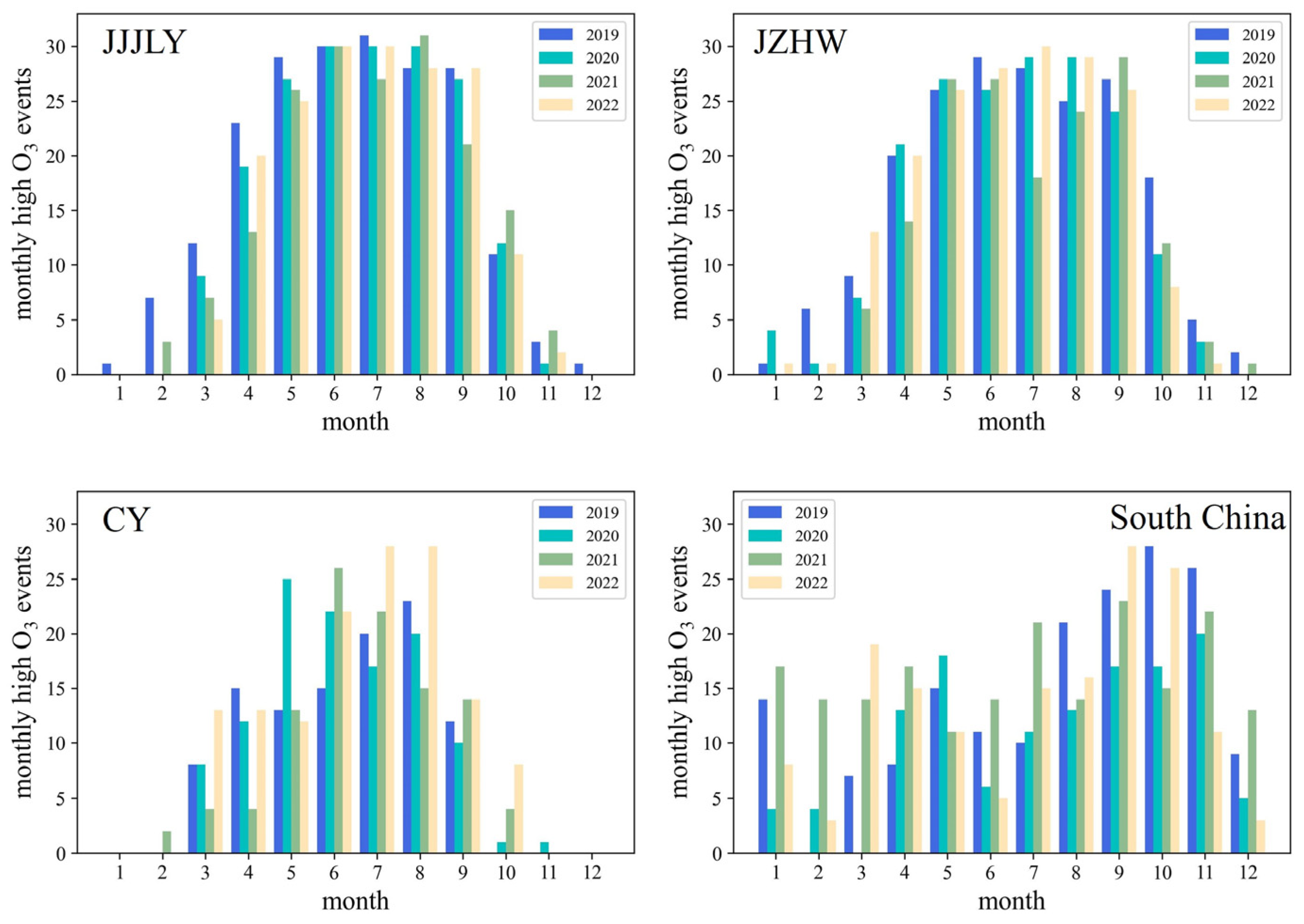
3.1.1. Analysis of O₃ pollution

Typical Chinese city clusters have distinct ozone pollution patterns, which are caused by the different meteorological factors [46]. In order to further explore the complex chemical-response relationship between O₃ and its precursors, and to assess the current O₃ pollution situations in representative regions of China, we utilized ground-based O₃ data to calculate the number of O₃ pollution days in different areas. We defined the ozone level as the daily maximum value of the maximum daily 8 h average ozone concentrations (MDA 8 h O₃) [47], and areas with values exceeding 160 μg/m³ were classified as experiencing O₃ pollution. Figure 2 presents the results of the O₃ pollution events (days) per month in the study areas. It is evident that regional differences in O₃ pollution exist. JJJLY, JZHW, and CY experience O₃ pollution mainly from May to September, which is the high-O₃-pollution period in China. Additionally, the South China regions primarily encounter O₃ pollution from August to October, as indicated by the local climatology. Among these regions, JJJLY exhibited the highest O₃ pollution due to both human activities and natural conditions. The peak months for O₃ pollution in JJJLY were July 2019 and August 2021, with 31 O₃ pollution days. In JZHW, the month with the most O₃ pollution days was July 2022 (30 days). In CY, the months with the most pollution days were July 2022 and August 2022 (28 days), and in South China, they were October 2019 and September 2022 (28 days). The O₃ pollution showed a declining trend from 2019 to 2020 but experienced an increase from 2021. The ozone pollution period was consistently observed from May to October each year.

3.1.2. Analysis of NO₂ and HCHO Pollution

Ozone pollution is closely linked to the pollution of the ozone precursors HCHO and NO₂. We analyzed the temporal and spatial variations in HCHO and NO₂ in the four study areas. Figure 3 displays the monthly average values of HCHO and NO₂ monitored by the TROPOMI, illustrating the monthly variation in these two precursors. During the ozone pollution period, the peak HCHO column density was recorded in 2019 for the JJJLY region, whereas for the JZHW, CY, and South China regions, the peak HCHO column densities occurred in 2022. Generally, JJJLY has the highest concentrations of HCHO and NO₂, while CY has the lowest concentrations. The variations in HCHO and NO₂ over time exhibit a relatively obvious periodicity.

High HCHO pollution tends to occur in June each year, with a second peak observed in October or November, and the tropospheric HCHO column densities in winter are significantly lower than those in summer. The highest tropospheric HCHO column densities in JJJLY, JZHW, CY, and South China were recorded in June 2019 (17.1 × 10¹⁵ molecules/cm²), August 2022 (16.2 × 10¹⁵ molecules/cm²), August 2022 (11 × 10¹⁵ molecules/cm²), and July 2021 (13.1 × 10¹⁵ molecules/cm²), respectively. The lowest column densities were observed in April 2021 (9.15 × 10¹⁵ molecules/cm²), January 2020 (8.77 × 10¹⁵ molecules/cm²), September 2019 (8.25 × 10¹⁵ molecules/cm²), and February 2019 (7.58 × 10¹⁵ molecules/cm²) for JJJLY, JZHW, CY, and South China, respectively.

NO₂ pollution exhibits opposite characteristics to HCHO pollution in terms of season. COVID-19 also impacted the NO₂ emissions from anthropogenic sources, leading to a significant reduction in the tropospheric NO₂ densities during the winter of 2019 compared to the same period in other years. The highest tropospheric NO₂ column densities in JJJLY, JZHW, CY, and South China were separately observed in December 2020 (17.5 × 10¹⁵ molecules/cm²), January 2019 (15.7 × 10¹⁵ molecules/cm²), December 2018 (6.11 × 10¹⁵ molecules/cm²), and December 2018 (4.2 × 10¹⁵ molecules/cm²). Conversely, the lowest tropospheric NO₂ densities in these regions occurred in August 2020 (2.98 × 10¹⁵ molecules/cm²), August 2019 (2.78 × 10¹⁵ molecules/cm²), August 2019 (1.35 × 10¹⁵ molecules/cm²), and July 2020 (1.54 × 10¹⁵ molecules/cm²), respectively.

Figure 4 displays the spatial characteristics of the average HCHO densities and average NO₂ densities from May to October, as monitored by the TROPOMI in JJJLY, JZHW, CY, and South China in 2022. From a spatial distribution perspective, it is indicated that the HCHO pollution and NO₂ pollution were mainly concentrated in urban areas with frequent human activities. The HCHO column densities were higher at the boundaries of Hebei, Henan, and Shandong provinces, as well as around the Yangtze River Delta and the Pearl River Delta in the JZHW and South China regions. High NO₂ values appeared near the downtown areas of several major cities, including Beijing, Tianjin, Shijiazhuang, and other densely populated cities or regions with well-developed economic and transportation activities.

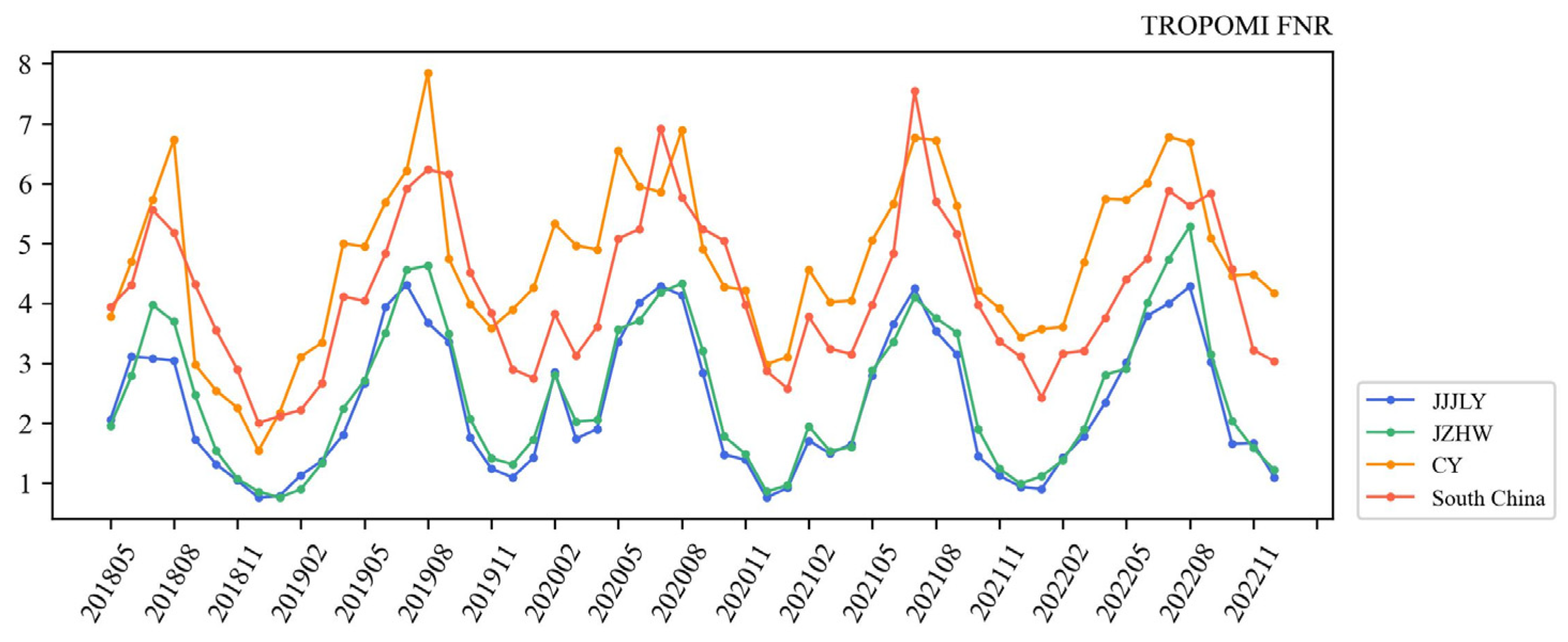
3.2. Regional and Seasonal Differences in FNR

The changes in O₃ and its precursors in the chemical-reaction process vary under different conditions. Therefore, when using the HCHO/NO₂ (FNR) method to determine the threshold, there are large considerable uncertainties arising from various meteorological factors and human activities. We utilized ground-based O₃ data from the environmental monitoring stations and correlated them with the ozone precursor indicator values (TROPOMI HCHO/TROPOMI NO₂) obtained from the satellite observations to assess the uncertainty of the FNR determination (Figure 5).

Figure 5 illustrates the seasonal and regional variation characteristics of the four representative regions in China (JJJLY, JZHW, CY, and South China) by matching the monthly mean values of the FNRs observed by satellite and the monthly mean values of the O₃ concentrations from ground-based data from May 2018 to December 2022. Different regions exhibit distinct FNR patterns and ozone concentrations, as indicated by the median data of their FNRs. Based on the median line and FNR distribution in Figure 5, the FNR values were generally higher in summer than those in other seasons. Except for the South China region, the FNR values in the other three regions were as follows: summer > spring > autumn > winter. However, in the South China region, the FNR values in autumn were slightly higher than those in spring. The highest value was recorded during the summer in South China (4.24), while the lowest value was observed during the winter in JJJLY (0.82). The seasonal differences in the FNR median values vary from 0.82 to 3.23 in JJJLY, from 0.83 to 3.06 in JZHW, from 1.46 to 3.68 in CY, and from 1.92 to 4.24 in South China. Furthermore, the sparsity of points in CY and South China is noticeably less than that in the other two regions, which may be attributed to the higher cloud coverage, leading to more invalid satellite observations.

There were evident regional differences in the FNRs. Based on the median line and FNR distribution, the FNR in South China was significantly higher than those in the other regions throughout all seasons. In spring and summer, the FNR values followed the order South China > CY > JJJLY > JZHW, while the FNR values in JJJLY were slightly lower than those in JZHW in autumn and winter. The FNR range in the South China area was larger compared to those of the other regions, which may also have contributed to the higher FNR median value.

The seasonal and regional differences in the FNRs prove the complex chemical reaction between O₃ and its precursors in the formation and transformation, and they are also the most intuitive manifestation of the FNR affected by precursor emissions and meteorological conditions. The FNR monitored in summer was higher than those in the other seasons. Additionally, the FNR median values in CY and South China were found to be higher than those in the other regions. These results can be attributed to higher levels of HCHO and lower levels of NO₂ (Figure 3).

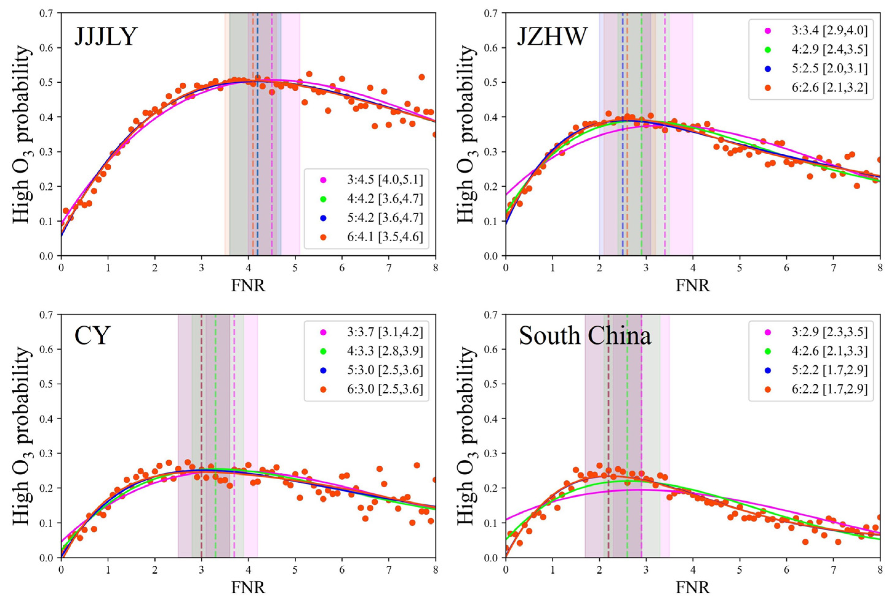
3.3. Determination and Analysis of FNR Thresholds for Ozone Precursors in Representative Areas

Figure 6a shows the relationship among the TROPOMI NO₂, TROPOMI HCHO, and ground-based O₃ concentrations in China from May 2018 to December 2022. The relationship observed was similar to the EKMA (Empirical Kinetic Modeling Approach) function, which describes the nonlinear interactions between HCHO, NO₂, and O₃. As a result, we considered the relationship among HCHO, NO₂, and O₃ to analyze the control area: When the FNR in a specific region was below the defined lower threshold, which means low HCHO densities and high NO₂ densities, and when, with the increase in the HCHO column densities, the O₃ concentrations increased more significantly, we classified this area as a VOC-limited regime. Conversely, if the FNR value in a region was higher than the upper threshold, the O₃ concentrations were more affected by NOx, so we classified it as a NOx-limited regime. Also, we considered areas falling between the FNR threshold as transitional regimes, in which the O₃ concentrations are controlled by both NOx and VOCs.

Because the O₃ pollution days in China always occurred from May to October, we selected the data in this period from 2018 to 2022 to determine the FNR thresholds. To ensure the accuracy of our results, we excluded data with O₃ sample quantities of less than 20 under one FNR, which could otherwise be influenced by a small sample size. Figure 6b illustrates the FNR determinations for JJJLY, JZHW, CY, and South China during the O₃ pollution period from 2018 to 2022 using third-degree polynomial fitting. Among the four representative regions, JJJLY had the highest FNR threshold, ranging from 4.0 to 5.1. CY followed with the second-highest FNR threshold, ranging from 3.1 to 4.2. The FNR threshold of JZHW ranged from 2.9 to 4.0, while the FNR threshold of South China was the lowest, ranging from 2.3 to 3.4. Due to the high cloud coverage in CY and South China, satellites may have difficulties accurately and effectively obtaining ground information, resulting in fewer valid data compared to other regions. The numbers of valid samples were 114,834 in JJJLY, 92,889 in JZHW, 32,454 in CY, and 62,886 in South China.

We noticed that the fitting degree may not be proper in different regions, especially in the CY and South China districts, where the fitted curve does not depict the change in the scatter well. We used polynomial fitting with degrees ranging from three to six to determine the FNR thresholds obtained by each of these polynomial fits, and we observed the differences between the results of each fit (Figure 7). To strike the balance between accurately describing the trend of change and avoiding overfitting, we selected the union of the results from the three–six polynomial fits as the threshold ranges of the FNRs. As a result, the FNR threshold for JJJLY was determined to be in the range of 3.5–5.1. For JZHW, the threshold falls within the range of 2.0–4.0. For CY, the range is 2.5–4.2, and for South China, it is 1.7–3.5. Compared to the threshold with a fitting order of 3 (Figure 6b), the new thresholds extend the FNR range by 0.5–0.9.

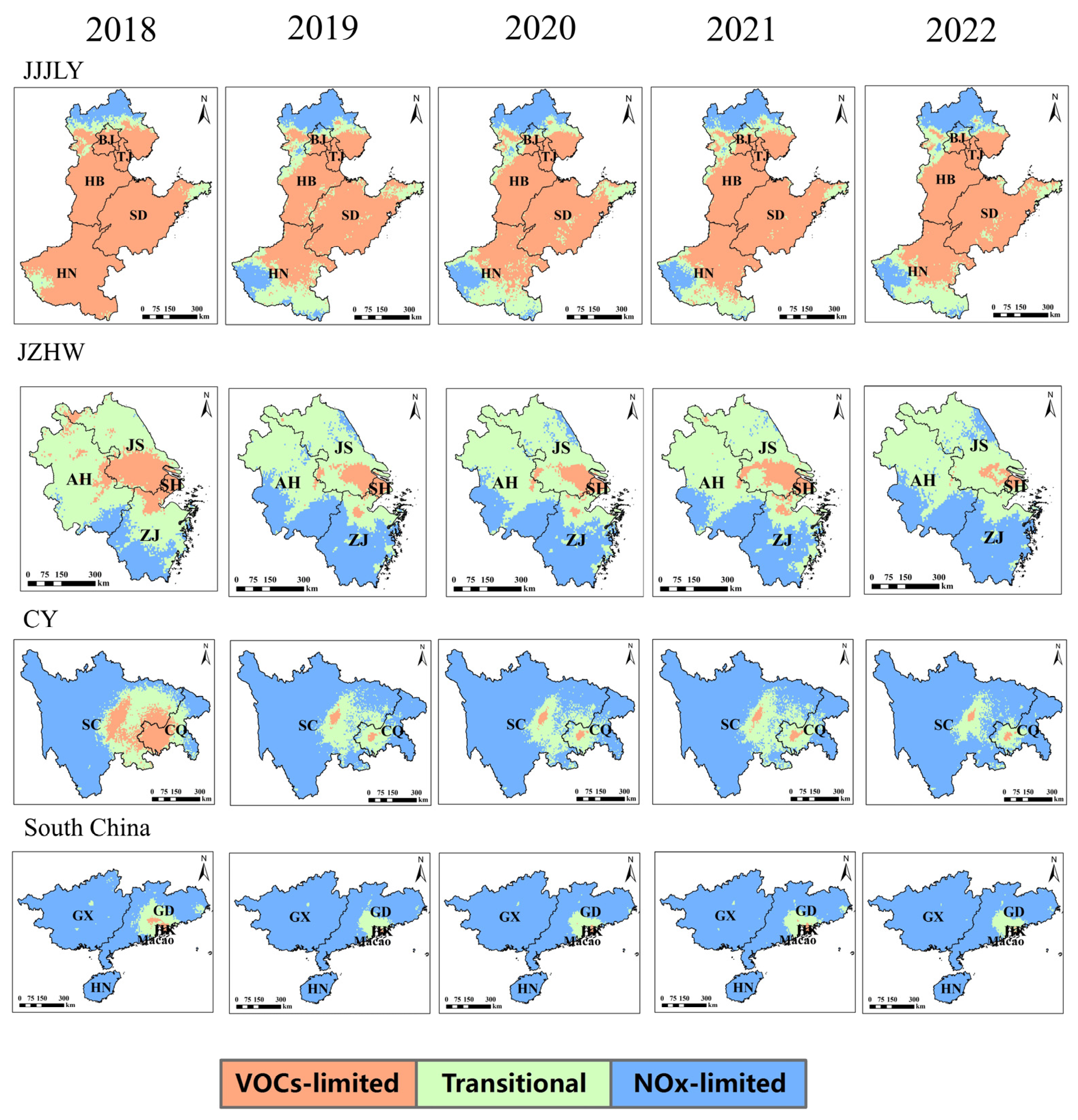
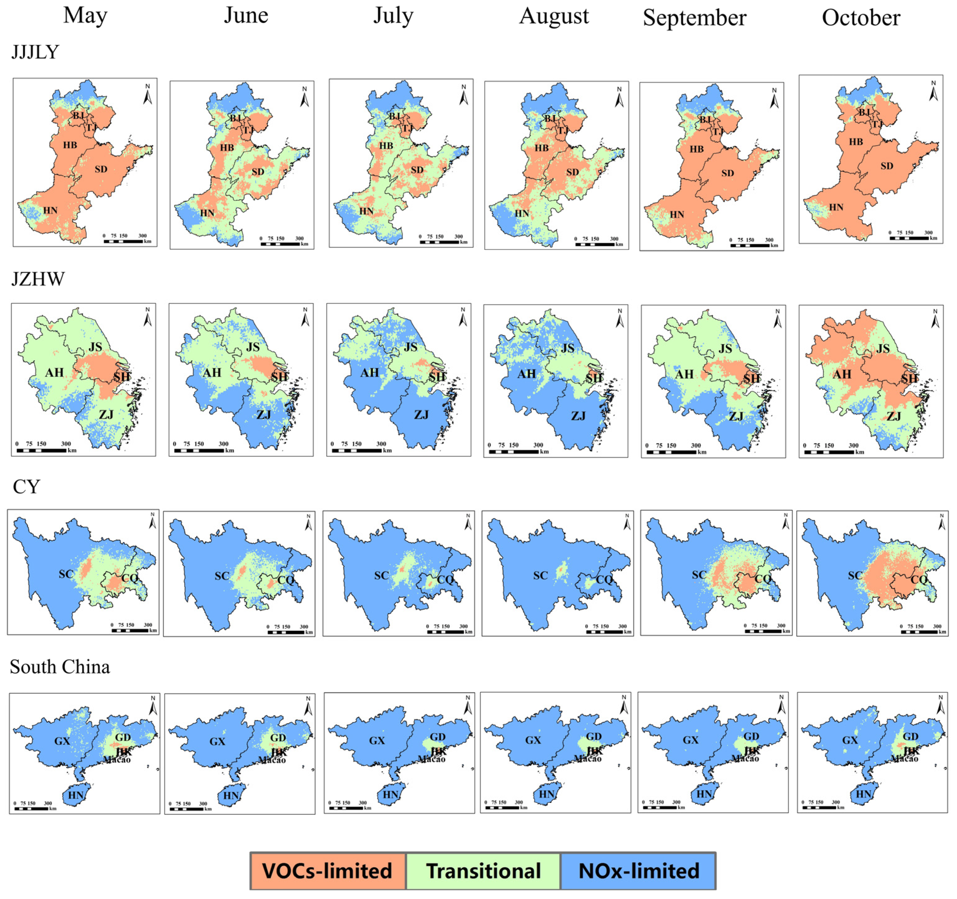
3.4. Spatial and Temporal Analysis of O₃ Control Regimes

To analyze the temporal characteristics of the FNR values, we calculated the monthly averaged FNR values of our four study areas (Figure 8). The analysis reveals distinct seasonal patterns in the variation in the FNRs, with higher values observed in summer and lower values in winter. The lowest FNR values occurred in December or January of each year. In addition to the peak FNR observed in July or August every year, there were slight rising peaks in February 2020 and February 2021. Overall, the FNRs in CY exhibited the highest values, followed by those of South China, while the FNR values in JJJLY and JZHW were lower. The highest FNR values in the JJJLY, JZHW, CY, and South China regions occurred in July 2019 (4.31), August 2018 (5.28), August 2019 (7.85), and July 2021 (7.54), respectively.

Based on the previously calculated FNR thresholds, we analyzed the spatial characteristics of the O₃ control regimes in JJJLY, JZHW, CY, and South China, as shown in Figure 9. The analysis revealed interesting trends in the control regimes from 2018 to 2022. Over this period, the areas classified as VOC-control regimes in our study areas gradually decreased, while there was a corresponding increase in the areas classified as transitional regimes. Additionally, some regions that were initially classified as transitional regimes changed to NOx-control regimes. Notably, VOC-limited regimes were predominantly observed in urban areas with more economic development and large populations, while NOx-limited regimes were mainly located in less developed areas [48]. In Figure 10, it is obvious that the VOC-limited regimes were mainly located on the North China Plain (NCP) and in the Yangtze River Delta (YRD), Pearl River Delta (PRD), and Chongqing. In contrast, Guangxi and western Sichuan, which represent less developed cities, fall into the NOx-limited regions.

In JJJLY, the majority of areas were primarily controlled by VOCs, indicating their association with more economically developed regions, including the southeast of Beijing, the entire area of Tianjin, the southern part of Hebei, the northern part of Henan, and the western areas of Shandong. Transitional areas in JJJLY were relatively scarce, while NOx-limited regimes were more prevalent in the northern part of Hebei and the southwest of Henan. Conversely, South China was mainly controlled by NOx, with the transitional regimes and VOC-limited regimes being less common. NOx-limited regimes were primarily located around the Guangdong–Hong Kong–Macao Greater Bay Area, which correspond to economically developed regions. In JZHW, the NOx-limited regimes experienced significant growth from 2018 to 2019 and remained relatively stable thereafter, and they were located in the south of Anhui and most areas of Zhejiang. While there was a slight growth trend in 2021 for the VOC-limited regimes, which were gradually reduced and converted into transitional regimes on the whole, this trend was mainly observed in Nanjing, Hefei, and the Yangtze River Delta. In CY, VOC-limited regimes mainly occurred in Chengdu and the main urban areas of Chongqing. The transitional regimes exhibited a radial distribution, while the majority of the areas in the region were classified as NOx-limited regimes.

Figure 10 shows the monthly distribution of the O₃ control areas in the years 2018–2022 from May to October. During the O₃ pollution period, the VOC-limited regimes in our four study areas initially decreased and gradually transformed into transitional regimes. Then, areas previously converted to transitional regimes were controlled by VOCs again in September, and even the VOC-limited regimes were further expanded in October, including some previous transitional regimes. The results indicated that the urban areas with faster economic development, such as Beijing, Tianjin, Shanghai, Chongqing, and Chengdu, were consistently controlled by VOCs, while the suburban areas of large cities exhibited a changing pattern, shifting from VOC-limited regimes to transitional regimes and then changing back to VOC-limited regimes, and the far suburbs were consistently controlled by NOx. Furthermore, we concluded that the smallest VOC-limited regimes in JJJLY and South China occurred in June, while those in JZHW and CY appeared in July. Based on our findings, it is possible to control the O₃ pollution in different locations at different times due to the variation in the O₃ control areas from month to month.

4. Discussion

Analyzing the sensitivity of the ozone formation in Chinese representative regions can help us to identify the main factors contributing to ozone pollution and take appropriate measures. The levels of O₃ pollution in JJJLY, JZHW, CY, and South China are severe (Figure 2). During the O₃ pollution period, high O3 concentrations can be observed in JJJLY and JZHW almost every day. Although the O₃ concentrations in CY and South China are relatively low compared to those in the other two regions, the O₃ pollution in major urban areas (Chongqing–Chengdu and the Pearl River Delta) is more severe than that in neighboring regions [47]. Furthermore, the O₃ concentrations in the Pearl River Delta increased at a rate of 0.28–1.02 ppb/yr from 2006 to 2019 [49], and high ozone concentrations of more than 160 μg/m³ have been observed frequently.

Also, the precursors of O₃, HCHO and NO₂, exhibited distinct seasonal variations. Higher concentrations of HCHO were observed in summer, while higher NO₂ concentrations were observed in winter. VOCs have complex sources, including biogenic sources, the petrochemical industry, and gasoline evaporation, among others. These sources tend to be higher in summer, resulting in the high levels of VOC pollution. In contrast, in winter, the aforementioned sources are reduced, while vehicular exhaust becomes the primary contributor [50]. Additionally, the tropical climate and evergreen forest in South China result in the continuous emissions of biogenic VOCs (BVOCs) throughout the year, leading to the reduced seasonality of HCHO in South China in this region [23]. The higher levels of NO₂ in winter could be attributed to several factors, including the height of the planetary-boundary layer, reduced sunlight, unique terrain, lower wind speeds, colder temperatures, higher humidity, and the burning of fossil fuels from human activities [51,52,53]. Lower densities typically occurred in summer with high temperatures, high humidity, a higher mixing-layer height, and a strong diffusion ability, which result in the short lifetime in summer [54,55,56].

The FNR values across different seasons and regions exhibited significant uncertainties and differences in the FNR values (Figure 5). The findings regarding the FNR thresholds in different areas indicated that the variations in the localized precursor emissions and meteorological conditions are the primary factors contributing to the differences in the FNR thresholds among the regions. The higher FNR threshold ranges observed in JJJLY and JZHW can be attributed to their more industrial economies. The validation characteristics (fitting-curve shape) of JZHW and CY were similar, possibly due to their similar latitudes, but with a higher value in CY. This could be the result of its unique basin topography and high humidity, which slow down the diffusion and dilution of precursors [57]. And the lowest FNR range in South China may be attributed to the fact that the period of high ozone pollution occurs relatively later compared to other regions (Figure 2). Additionally, we observed that the sampling quantity also influenced the determination of the threshold values.

The spatial characteristics of the ozone control areas indicated that urban areas with industrial activities and dense populations were primarily under VOC-limited regimes, while suburban areas predominantly fell within transitional regimes. Rural and other remote areas with fewer human activities were mainly controlled by NOx, which is consistent with the findings of Shen et al. [48] and Wang et al. [21]. During the period of O₃ pollution, the urban areas in the four representative regions shifted from VOC-limited regimes to transitional regimes, and some transitional regimes in the suburban areas changed to NOx-limited regimes. Subsequently, most areas that were previously jointly controlled by VOCs and NOx shifted to VOC-limited regimes. Cities with rapid economic development were consistently controlled by VOCs. Because the types of O₃ control areas vary depending on time and location, it is possible to control the O₃ pollution at different locations and during different periods.

It should be noted that this study still has certain limitations. Firstly, the quality of the satellite data, especially the accuracy of the HCHO retrieval, will ultimately determine the precision of the FNR threshold determination [58]. Additionally, the formation of surface O₃ occurs after the formation of its precursors, requiring a chemical-reaction process. This can provide uncertainties in using polar-orbiting satellite data and ground-based data [42,43]. In the future, using geostationary satellite data may alleviate this issue and enhance our understanding of the formation of O₃ and its precursors.

5. Conclusions

In this work, we investigated the relationships between ozone (O₃) and its precursors by analyzing the tropospheric HCHO column densities and tropospheric NO₂ column densities from May 2018 to December 2022, as monitored by the TROPOMI. We combined these satellite data with ground-based O₃ monitoring data to analyze the sensitivity of the O₃ formation in four representative regions in China: JJJLY, JZHW, CY, and South China.

The results revealed clear cyclical patterns in both the tropospheric HCHO and NO₂ concentrations. Higher HCHO column densities were consistently observed during the summer months, while higher NO₂ levels were predominant in winter. By correlating ground-based O₃ measurements with HCHO/NO₂ data collected from the TROPOMI, we evaluated the differences in the FNRs and ozone concentrations across different regions and seasons. The variations in the FNRs demonstrated the complex interplay of the pollution sources of O₃, highlighting the importance of establishing local ozone control areas. We identified the FNR thresholds for four representative regions in China: JJJLY, JZHW, CY, and South China. The FNR thresholds for each region were from 3.5 to 5.0, from 2.1 to 4.0, from 2.3 to 4.4, and from 1.6 to 3.6, respectively.

Furthermore, we analyzed the spatial and temporal characteristics of the ozone control areas. We observed periodic variations in the FNR values, as monitored by satellites, with higher values in summer and lower values in winter. By applying the previously determined FNR thresholds, we classified the ozone precursor control areas into four representative regions. The smallest VOC-limited regimes were observed in JJJLY and South China in June, while in JZHW and CY, they occurred in July. VOC-limited regions were mainly observed in urban areas with developed industrial economies and dense populations, while rural regions with less developed economies were mainly controlled by NOx. Dynamic shifts were observed during the ozone pollution period. Urban areas shifted from being controlled by VOCs to transitional regimes, while suburban areas transitioned from transitional regimes to being controlled by NOx. Eventually, these changes reverted back to their previous control types. Areas with developed industrial economies were consistently controlled by VOCs.

In summary, we determined the FNR thresholds for four representative regions in China and evaluated the sensitivity of the ozone formation using ground-based data and TROPOMI data. Additionally, we analyzed the spatial and temporal features of the HCHO, NO₂, and ozone control areas. Our findings offer valuable insights for initiatives aimed at controlling ozone pollution and enhance our understanding of the mechanisms behind ozone formation and the contributions of different precursors in various regions.

References

1. Nuvolone, D.; Petri, D.; Voller, F. The Effects of Ozone on Human Health. Environ. Sci. Pollut. Res. 2018, 25, 8074–8088. [Google Scholar] [CrossRef] [PubMed]
2. Norval, M.; Cullen, A.P.; De Gruijl, F.R.; Longstreth, J.; Takizawa, Y.; Lucas, R.M.; Noonan, F.P.; Van Der Leun, J.C. The Effects on Human Health from Stratospheric Ozone Depletion and Its Interactions with Climate Change. Photochem. Photobiol. Sci. 2007, 6, 232–251. [Google Scholar] [CrossRef] [PubMed]
3. Zhao, F.; Liu, C.; Cai, Z.; Liu, X.; Bak, J.; Kim, J.; Hu, Q.; Xia, C.; Zhang, C.; Sun, Y.; et al. Ozone Profile Retrievals from TROPOMI: Implication for the Variation of Tropospheric Ozone during the Outbreak of COVID-19 in China. Sci. Total Environ. 2021, 764, 142886. [Google Scholar] [CrossRef] [PubMed]
4. Haagen-Smit, A.J. Chemistry and Physiology of Los Angeles Smog. Ind. Eng. Chem. 1952, 44, 1342–1346. [Google Scholar] [CrossRef]
5. Feng, Y.; Ning, M.; Lei, Y.; Sun, Y.; Liu, W.; Wang, J. Defending Blue Sky in China: Effectiveness of the “Air Pollution Prevention and Control Action Plan” on Air Quality Improvements from 2013 to 2017. J. Environ. Manag. 2019, 252, 109603. [Google Scholar] [CrossRef] [PubMed]
6. Liu, C.; Xing, C.; Hu, Q.; Li, Q.; Liu, H.; Hong, Q.; Tan, W.; Ji, X.; Lin, H.; Lu, C.; et al. Ground-Based Hyperspectral Stereoscopic Remote Sensing Network: A Promising Strategy to Learn Coordinated Control of O3 and PM2.5 over China. Engineering 2022, 19, 71–83. [Google Scholar] [CrossRef]
7. Wang, T.; Xue, L.; Brimblecombe, P.; Lam, Y.F.; Li, L.; Zhang, L. Ozone Pollution in China: A Review of Concentrations, Meteorological Influences, Chemical Precursors, and Effects. Sci. Total Environ. 2017, 575, 1582–1596. [Google Scholar] [CrossRef]
8. Nguyen, D.-H.; Lin, C.; Vu, C.-T.; Cheruiyot, N.K.; Nguyen, M.K.; Le, T.H.; Lukkhasorn, W.; Vo, T.-D.-H.; Bui, X.-T. Tropospheric Ozone and NOx: A Review of Worldwide Variation and Meteorological Influences. Environ. Technol. Innov. 2022, 28, 102809. [Google Scholar] [CrossRef]
9. Lal, S.; Naja, M.; Subbaraya, B.H. Seasonal Variations in Surface Ozone and Its Precursors over an Urban Site in India. Atmos. Environ. 2000, 34, 2713–2724. [Google Scholar] [CrossRef]
10. Sillman, S. Some Theoretical Results Concerning O3-NOx-VOC Chemistry and NOx-VOC Indicators. J. Geophys. Res. 2002, 107, 4659. [Google Scholar] [CrossRef]
11. Wang, X.; Yin, S.; Zhang, R.; Yuan, M.; Ying, Q. Assessment of Summertime O3 Formation and the O3-NOx-VOC Sensitivity in Zhengzhou, China Using an Observation-Based Model. Sci. Total Environ. 2022, 813, 152449. [Google Scholar] [CrossRef]
12. Choi, Y.; Kim, H.; Tong, D.; Lee, P. Summertime Weekly Cycles of Observed and Modeled NOx and O3 Concentrations as a Function of Satellite-Derived Ozone Production Sensitivity and Land Use Types over the Continental United States. Atmos. Chem. Phys. 2012, 12, 6291–6307. [Google Scholar] [CrossRef]
13. Sun, J.; Shen, Z.; Wang, R.; Li, G.; Zhang, Y.; Zhang, B.; He, K.; Tang, Z.; Xu, H.; Qu, L.; et al. A Comprehensive Study on Ozone Pollution in a Megacity in North China Plain during Summertime: Observations, Source Attributions and Ozone Sensitivity. Environ. Int. 2021, 146, 106279. [Google Scholar] [CrossRef] [PubMed]
14. Xie, M.; Zhu, K.; Wang, T.; Yang, H.; Zhuang, B.; Li, S.; Li, M.; Zhu, X.; Ouyang, Y. Application of Photochemical Indicators to Evaluate Ozone Nonlinear Chemistry and Pollution Control Countermeasure in China. Atmos. Environ. 2014, 99, 466–473. [Google Scholar] [CrossRef]
15. Sillman, S. The Use of NOy, H2O2, and HNO3 as Indicators for Ozone-NOx-Hydrocarbon Sensitivity in Urban Locations. J. Geophys. Res. 1995, 100, 14175. [Google Scholar] [CrossRef]
16. Tonnesen, G.S.; Dennis, R.L. Analysis of Radical Propagation Efficiency to Assess Ozone Sensitivity to Hydrocarbons and NOx: 1. Local Indicators of Instantaneous Odd Oxygen Production Sensitivity. J. Geophys. Res. Atmos. 2000, 105, 9213–9225. [Google Scholar] [CrossRef]
17. Liu, J.; Li, X.; Tan, Z.; Wang, W.; Yang, Y.; Zhu, Y.; Yang, S.; Song, M.; Chen, S.; Wang, H.; et al. Assessing the Ratios of Formaldehyde and Glyoxal to NO2 as Indicators of O3–NOx–VOC Sensitivity. Environ. Sci. Technol. 2021, 55, 10935–10945. [Google Scholar] [CrossRef]
18. Martin, R.V.; Fiore, A.M.; Van Donkelaar, A. Space-Based Diagnosis of Surface Ozone Sensitivity to Anthropogenic Emissions: Surface Ozone Sensitivity to Emissions. Geophys. Res. Lett. 2004, 31, L06120. [Google Scholar] [CrossRef]
19. Duncan, B.N.; Yoshida, Y.; Olson, J.R.; Sillman, S.; Martin, R.V.; Lamsal, L.; Hu, Y.; Pickering, K.E.; Retscher, C.; Allen, D.J.; et al. Application of OMI Observations to a Space-Based Indicator of NOx and VOC Controls on Surface Ozone Formation. Atmos. Environ. 2010, 44, 2213–2223. [Google Scholar] [CrossRef]
20. Jin, X.; Fiore, A.; Boersma, K.F.; Smedt, I.D.; Valin, L. Inferring Changes in Summertime Surface Ozone–NOx–VOC Chemistry over U.S. Urban Areas from Two Decades of Satellite and Ground-Based Observations. Environ. Sci. Technol. 2020, 54, 6518–6529. [Google Scholar] [CrossRef]
21. Wang, W.; van der A, R.; Ding, J.; van Weele, M.; Cheng, T. Spatial and Temporal Changes of the Ozone Sensitivity in China Based on Satellite and Ground-Based Observations. Atmos. Chem. Phys. 2021, 21, 7253–7269. [Google Scholar] [CrossRef]
22. Choi, Y.; Souri, A.H. Chemical Condition and Surface Ozone in Large Cities of Texas during the Last Decade: Observational Evidence from OMI, CAMS, and Model Analysis. Remote Sens. Environ. 2015, 168, 90–101. [Google Scholar] [CrossRef]
23. Jin, X.; Holloway, T. Spatial and Temporal Variability of Ozone Sensitivity over China Observed from the Ozone Monitoring Instrument: Ozone Sensitivity over China. J. Geophys. Res. Atmos. 2015, 120, 7229–7246. [Google Scholar] [CrossRef]
24. Witte, J.C.; Duncan, B.N.; Douglass, A.R.; Kurosu, T.P.; Chance, K.; Retscher, C. The Unique OMI HCHO/NO2 Feature during the 2008 Beijing Olympics: Implications for Ozone Production Sensitivity. Atmos. Environ. 2011, 45, 3103–3111. [Google Scholar] [CrossRef]
25. Chen, Y.; Yan, H.; Yao, Y.; Zeng, C.; Gao, P.; Zhuang, L.; Fan, L.; Ye, D. Relationships of Ozone Formation Sensitivity with Precursors Emissions, Meteorology and Land Use Types, in Guangdong-Hong Kong-Macao Greater Bay Area, China. J. Environ. Sci. 2020, 94, 1–13. [Google Scholar] [CrossRef] [PubMed]
26. Sun, Y.; Liu, C.; Palm, M.; Vigouroux, C.; Notholt, J.; Hu, Q.; Jones, N.; Wang, W.; Su, W.; Zhang, W.; et al. Ozone Seasonal Evolution and Photochemical Production Regime in the Polluted Troposphere in Eastern China Derived from High-Resolution Fourier Transform Spectrometry (FTS) Observations. Atmos. Chem. Phys. 2018, 18, 14569–14583. [Google Scholar] [CrossRef]
27. Li, Y.; Yin, S.; Yu, S.; Bai, L.; Wang, X.; Lu, X.; Ma, S. Characteristics of Ozone Pollution and the Sensitivity to Precursors during Early Summer in Central Plain, China. J. Environ. Sci. 2021, 99, 354–368. [Google Scholar] [CrossRef]
28. Lu, C.; Chang, J.S. On the Indicator-based Approach to Assess Ozone Sensitivities and Emissions Features. J. Geophys. Res. Atmos. 1998, 103, 3453–3462. [Google Scholar] [CrossRef]
29. Sun, H.Z.; Zhao, J.; Liu, X.; Qiu, M.; Shen, H.; Guillas, S.; Giorio, C.; Staniaszek, Z.; Yu, P.; Wan, M.W.L.; et al. Antagonism between Ambient Ozone Increase and Urbanization-Oriented Population Migration on Chinese Cardiopulmonary Mortality. Innovation 2023, 4, 100517. [Google Scholar] [CrossRef]
30. De Smedt, I.; Pinardi, G.; Vigouroux, C.; Compernolle, S.; Bais, A.; Benavent, N.; Boersma, F.; Chan, K.-L.; Donner, S.; Eichmann, K.-U.; et al. Comparative Assessment of TROPOMI and OMI Formaldehyde Observations and Validation against MAX-DOAS Network Column Measurements. Atmos. Chem. Phys. 2021, 21, 12561–12593. [Google Scholar] [CrossRef]
31. Huang, G.; Sun, K. Non-Negligible Impacts of Clean Air Regulations on the Reduction of Tropospheric NO2 over East China during the COVID-19 Pandemic Observed by OMI and TROPOMI. Sci. Total Environ. 2020, 745, 141023. [Google Scholar] [CrossRef] [PubMed]
32. Van Geffen, J.; Eskes, H.; Compernolle, S.; Pinardi, G.; Verhoelst, T.; Lambert, J.-C.; Sneep, M.; Ter Linden, M.; Lu-dewig, A.; Boersma, K.F.; et al. Sentinel-5P TROPOMI NO2 Retrieval: Impact of Version v2.2 Improvements and Comparisons with OMI and Ground-Based Data. Atmos. Meas. Tech. 2022, 15, 2037–2060. [Google Scholar] [CrossRef]
33. Shikwambana, L.; Mhangara, P.; Mbatha, N. Trend Analysis and First Time Observations of Sulphur Dioxide and Nitrogen Dioxide in South Africa Using TROPOMI/Sentinel-5 P Data. Int. J. Appl. Earth Obs. Geoinf. 2020, 91, 102130. [Google Scholar] [CrossRef]
34. Veefkind, J.P.; Aben, I.; McMullan, K.; Förster, H.; de Vries, J.; Otter, G.; Claas, J.; Eskes, H.J.; de Haan, J.F.; Kleipool, Q.; et al. TROPOMI on the ESA Sentinel-5 Precursor: A GMES Mission for Global Observations of the Atmospheric Composition for Climate, Air Quality and Ozone Layer Applications. Remote Sens. Environ. 2012, 120, 70–83. [Google Scholar] [CrossRef]
35. Vigouroux, C.; Langerock, B.; Bauer Aquino, C.A.; Blumenstock, T.; Cheng, Z.; De Mazière, M.; De Smedt, I.; Grutter, M.; Hannigan, J.W.; Jones, N.; et al. TROPOMI–Sentinel-5 Precursor Formaldehyde Validation Using an Extensive Network of Ground-Based Fourier-Transform Infrared Stations. Atmos. Meas. Tech. 2020, 13, 3751–3767. [Google Scholar] [CrossRef]
36. Verhoelst, T.; Compernolle, S.; Pinardi, G.; Lambert, J.-C.; Eskes, H.J.; Eichmann, K.-U.; Fjæraa, A.M.; Granville, J.; Niemeijer, S.; Cede, A.; et al. Ground-Based Validation of the Copernius Sentinel-5P TROPOMI NO2 Measurements with the NDACC ZSL-DOAS, MAX-DOAS and Pandonia Global Networks. Atmos. Meas. Tech. 2021, 14, 481–510. [Google Scholar] [CrossRef]
37. Copernicus Sentinel Data Processed by ESA, German Aerospace Center (DLR) (2020), Sentinel-5P TROPOMI Tropospheric Formaldehyde HCHO 1-Orbit L2 5.5 km × 3.5 km, Greenbelt, MD, USA, Goddard Earth Sciences Data and Information Services Center (GES DISC), 10.5270/S5P-vg1i7t0. Available online: https://disc.gsfc.nasa.gov/datasets/S5P_L2__HCHO___HiR_2/summary (accessed on 9 August 2023).
38. Copernicus Sentinel data processed by ESA, Koninklijk Nederlands Meteorologisch Instituut (KNMI) (2021), Sentinel-5P TROPOMI Tropospheric NO2 1-Orbit L2 5.5 km × 3.5 km, Greenbelt, MD, USA, Goddard Earth Sciences Data and Information Services Center (GES DISC), 10.5270/S5P-9bnp8q8. Available online: https://disc.gsfc.nasa.gov/datasets/S5P_L2__NO2____HiR_2/summary (accessed on 9 August 2023).
39. Zhang, Y.-L.; Cao, F. Fine Particulate Matter (PM2.5) in China at a City Level. Sci. Rep. 2015, 5, 14884. [Google Scholar] [CrossRef]
40. Zhang, C.; Liu, C.; Li, B.; Zhao, F.; Zhao, C. Spatiotemporal Neural Network for Estimating Surface NO2 Concentrations over North China and Their Human Health Impact. Environ. Pollut. 2022, 307, 119510. [Google Scholar] [CrossRef]
41. Lin, H.; Xing, C.; Hong, Q.; Liu, C.; Ji, X.; Liu, T.; Lin, J.; Lu, C.; Tan, W.; Li, Q.; et al. Diagnosis of Ozone Formation Sensitivities in Different Height Layers via MAX-DOAS Observations in Guangzhou. J. Geophys. Res. Atmos. 2022, 127, e2022JD036803. [Google Scholar] [CrossRef]
42. Zhang, K.; Li, L.; Huang, L.; Wang, Y.; Huo, J.; Duan, Y.; Wang, Y.; Fu, Q. The Impact of Volatile Organic Compounds on Ozone Formation in the Suburban Area of Shanghai. Atmos. Environ. 2020, 232, 117511. [Google Scholar] [CrossRef]
43. Han, S.; Bian, H.; Feng, Y.; Liu, A.; Li, X.; Zeng, F.; Zhang, X. Analysis of the Relationship between O3, NO and NO2 in Tianjin, China. Aerosol Air Qual. Res. 2011, 11, 128–139. [Google Scholar] [CrossRef]
44. Li, P.; De Marco, A.; Feng, Z.; Anav, A.; Zhou, D.; Paoletti, E. Nationwide Ground-Level Ozone Measurements in China Suggest Serious Risks to Forests. Environ. Pollut. 2018, 237, 803–813. [Google Scholar] [CrossRef] [PubMed]
45. GB3095-2012; Ambient Air Quality Standard. Ministry of Ecology and Environment of the People’s Republic of China: Beijing, China, 2012. (In Chinese)
46. Wang, W.; Parrish, D.D.; Wang, S.; Bao, F.; Ni, R.; Li, X.; Yang, S.; Wang, H.; Cheng, Y.; Su, H. Long-Term Trend of Ozone Pollution in China during 2014–2020: Distinct Seasonal and Spatial Characteristics and Ozone Sensitivity. Atmos. Chem. Phys. 2022, 22, 8935–8949. [Google Scholar] [CrossRef]
47. Yang, G.; Liu, Y.; Li, X. Spatiotemporal Distribution of Ground-Level Ozone in China at a City Level. Sci. Rep. 2020, 10, 7229. [Google Scholar] [CrossRef] [PubMed]
48. Shen, H.; Sun, Z.; Chen, Y.; Russell, A.G.; Hu, Y.; Odman, M.T.; Qian, Y.; Archibald, A.T.; Tao, S. Novel Method for Ozone Isopleth Construction and Diagnosis for the Ozone Control Strategy of Chinese Cities. Environ. Sci. Technol. 2021, 55, 15625–15636. [Google Scholar] [CrossRef]
49. Li, X.-B.; Yuan, B.; Parrish, D.D.; Chen, D.; Song, Y.; Yang, S.; Liu, Z.; Shao, M. Long-Term Trend of Ozone in Southern China Reveals Future Mitigation Strategy for Air Pollution. Atmos. Environ. 2022, 269, 118869. [Google Scholar] [CrossRef]
50. Xu, Z.; Zou, Q.; Jin, L.; Shen, Y.; Shen, J.; Xu, B.; Qu, F.; Zhang, F.; Xu, J.; Pei, X.; et al. Characteristics and Sources of Ambient Volatile Organic Compounds (VOCs) at a Regional Background Site, YRD Region, China: Significant Influence of Solvent Evaporation during Hot Months. Sci. Total Environ. 2023, 857, 159674. [Google Scholar] [CrossRef]
51. Yang, J.; Kang, S.; Ji, Z.; Yin, X.; Tripathee, L. Investigating Air Pollutant Concentrations, Impact Factors, and Emission Control Strategies in Western China by Using a Regional Climate-Chemistry Model. Chemosphere 2020, 246, 125767. [Google Scholar] [CrossRef]
52. Zhang, H.; Wang, Y.; Hu, J.; Ying, Q.; Hu, X.-M. Relationships between Meteorological Parameters and Criteria Air Pollutants in Three Megacities in China. Environ. Res. 2015, 140, 242–254. [Google Scholar] [CrossRef]
53. Jin, L.; Berman, J.D.; Zhang, Y.; Thurston, G.; Zhang, Y.; Bell, M.L. Land Use Regression Study in Lanzhou, China: A Pilot Sampling and Spatial Characteristics of Pilot Sampling Sites. Atmos. Environ. 2019, 210, 253–262. [Google Scholar] [CrossRef]
54. Liu, Y.; Zhao, J.; Song, K.; Cheng, C.; Li, S.; Cai, K. Spatiotemporal Evolution Analysis of NO2 Column Density before and after COVID-19 Pandemic in Henan Province Based on SI-APSTE Model. Sci. Rep. 2021, 11, 18614. [Google Scholar] [CrossRef] [PubMed]
55. Tang, G.; Zhang, J.; Zhu, X.; Song, T.; Münkel, C.; Hu, B.; Schäfer, K.; Liu, Z.; Zhang, J.; Wang, L.; et al. Mixing Layer Height and Its Implications for Air Pollution over Beijing, China. Atmos. Chem. Phys. 2016, 16, 2459–2475. [Google Scholar] [CrossRef]
56. Wagner, P.; Schäfer, K. Influence of Mixing Layer Height on Air Pollutant Concentrations in an Urban Street Canyon. Urban Clim. 2017, 22, 64–79. [Google Scholar] [CrossRef]
57. Chen, Y.; Wang, M.; Yao, Y.; Zeng, C.; Zhang, W.; Yan, H.; Gao, P.; Fan, L.; Ye, D. Research on the Ozone Formation Sensitivity Indicator of Four Urban Agglomerations of China Using Ozone Monitoring Instrument (OMI) Satellite Data and Ground-Based Measurements. Sci. Total Environ. 2023, 869, 161679. [Google Scholar] [CrossRef]
58. Chan, K.L.; Wiegner, M.; van Geffen, J.; De Smedt, I.; Alberti, C.; Cheng, Z.; Ye, S.; Wenig, M. MAX-DOAS Measurements of Tropospheric NO2 and HCHO in Munich and the Comparison to OMI and TROPOMI Satellite Observations. Atmos. Meas. Tech. 2020, 13, 4499–4520. [Google Scholar] [CrossRef]
Figure 1. Distribution of four city clusters selected in our study (JJJLY: Beijing–Tianjin–Hebei–Shandong–Henan; JZHW: Jiangsu–Zhejiang–Shanghai–Anhui; CY: Sichuan–Chongqing; South China: Guangdong–Guangxi–Hainan–Hong Kong–Macao) and environmental monitoring stations (national control points) in China.
Remotesensing 16 00316 g001
Figure 2. Monthly O3 pollution events (MDA 8 h O3 above 160 μg/m3) monitored via ground-based CNEMC data in JJJLY, JZHW, CY, and South China from 2019 to 2022.
Remotesensing 16 00316 g002
Figure 3. Temporal variation in tropospheric HCHO column concentrations and NO2 column concentrations from May 2018 to 2022 in JJJLY, JZHW, CY, and South China.
Remotesensing 16 00316 g003
Figure 4. Spatial distributions of average HCHO column densities and NO2 column densities in JJJLY, JZHW, CY, and South China during ozone pollution period (from May to October) in 2022. The labels in the figure represent various locations, such as Beijing (BJ), Tianjin (TJ), Hebei (HB), Shandong (SD), Henan (HN), Anhui (AH), Jiangsu (JS), Zhejiang (ZJ), Shanghai (SH), Sichuan (SC), Chongqing (CQ), Guangxi (GX), Guangdong (GD), Hong Kong (HK), and Hainan (HN).
Remotesensing 16 00316 g004
Figure 5. Uncertainty in determining FNR thresholds (average monthly data were used for calculation). The dotted line is the median of the FNR in different seasons, including MAM: March–April–May; JJA: June–July–August; SON: September–October–November; and DJF: December–January–February; the median represents the aggregation degree of the data.
Remotesensing 16 00316 g005
Figure 6. Determination of FNR threshold: (a) relationship of NO2, HCHO, and O3 concentrations in China from May 2018 to December 2022; red, green, and blue lines represent O3 concentrations of 100 μg/m3, 130 μg/m3, and 160 μg/m3, respectively; (b) fitting functions of FNRs to determine the FNR thresholds with third-degree polynomial fitting in JJJLY, JZHW, CY, and South China, using data from May to October in 2018–2022.
Remotesensing 16 00316 g006
Figure 7. FNR threshold results obtained via third–sixth-degree polynomial fittings in JJJLY, JZHW, CY, and South China. Pink plots and line denote the results from the third-degree polynomial fitting; green color denotes results from the fourth-degree polynomial fitting; blue color denotes results from the fifth-degree polynomial fitting; and orange color denotes results from the sixth-degree polynomial fitting.
Remotesensing 16 00316 g007
Figure 8. Monthly mean values of FNRs of JJJLY, JZHW, CY, and South China from May 2018 to December 2022.
Remotesensing 16 00316 g008
Figure 9. Yearly photochemical-regime classification over study areas in O3 pollution period from 2018 to 2022.
Remotesensing 16 00316 g009
Figure 10. Monthly photochemical-regime classification over study areas in 2018–2022 from May to October.
Remotesensing 16 00316 g010
Disclaimer/Publisher’s Note: The statements, opinions and data contained in all publications are solely those of the individual author(s) and contributor(s) and not of MDPI and/or the editor(s). MDPI and/or the editor(s) disclaim responsibility for any injury to people or property resulting from any ideas, methods, instructions or products referred to in the content.