Article

Automatic Detection of Phytophthora pluvialis Outbreaks in Radiata Pine Plantations Using Multi-Scene, Multi-Temporal Satellite Imagery

1
Scion, Titokorangi Drive, Private Bag 3020, Rotorua 3046, New Zealand
2
College of Science and Engineering, Flinders University, Sturt Rd, Bedford Park 5042, Australia
3
Scion, 10 Kyle Street, Christchurch 8011, New Zealand
*
Author to whom correspondence should be addressed.
Remote Sens. 2024, 16(2), 338; https://doi.org/10.3390/rs16020338
Submission received: 6 November 2023 / Revised: 7 January 2024 / Accepted: 11 January 2024 / Published: 15 January 2024
(This article belongs to the Section Forest Remote Sensing)

Abstract

:
This study demonstrates a framework for using high-resolution satellite imagery to automatically map and monitor outbreaks of red needle cast (Phytophthora pluvialis) in planted pine forests. This methodology was tested on five WorldView satellite scenes collected over two sites in the Gisborne Region of New Zealand’s North Island. All scenes were acquired in September: four scenes were acquired yearly (2018–2020 and 2022) for Wharerata, while one more was obtained in 2019 for Tauwhareparae. Training areas were selected for each scene using manual delineation combined with pixel-level thresholding rules based on band reflectance values and vegetation indices (selected empirically) to produce ‘pure’ training pixels for the different classes. A leave-one-scene-out, pixel-based random forest classification approach was then used to classify all images into (i) healthy pine forest, (ii) unhealthy pine forest or (iii) background. The overall accuracy of the models on the internal validation dataset ranged between 92.1% and 93.6%. Overall accuracies calculated for the left-out scenes ranged between 76.3% and 91.1% (mean overall accuracy of 83.8%), while user’s and producer’s accuracies across the three classes were 60.2–99.0% (71.4–91.8% for unhealthy pine forest) and 54.4–100% (71.9–97.2% for unhealthy pine forest), respectively. This work demonstrates the possibility of using a random forest classifier trained on a set of satellite scenes for the classification of healthy and unhealthy pine forest in new and completely independent scenes. This paves the way for a scalable and largely autonomous forest health monitoring system based on annual acquisitions of high-resolution satellite imagery at the time of peak disease expression, while greatly reducing the need for manual interpretation and delineation.

Graphical Abstract

1. Introduction

Ongoing global climate change is increasingly exposing the world’s forests to unprecedented levels of abiotic and biotic threats [1,2,3]. Continual increases in global trade and international travel, together with the lack of adequate quarantine policies and biosecurity regulations in many countries, have favored the introduction (whether intentional or otherwise) of alien invasive species that may be dangerous for local environments [4,5]. Thus, the distributions of many non-native plants [6,7], forest insects [8], and plant pathogens [9,10] have been artificially expanded largely beyond their natural boundaries, with, in some cases, large disturbances to the affected ecosystems and severe socio-economic impacts [11,12]. Among these impacts, alien plant pathogen invaders are particularly dangerous, since they can have major detrimental effects on plants, animals, and ecosystem health [13,14], as well as the often prohibitive costs involved in their management and the economic damage they can cause [15,16].
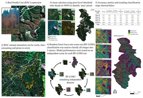
Red needle cast (RNC) is a foliar disease of radiata pine (Pinus radiataFigure 1), caused by the oomycete pathogen Phytophthora pluvialis and, occasionally, by Phytophthora kernoviae [17]. Phytophthora pluvialis was first recorded in New Zealand in 2008 [17], while P. kernoviae is known to have been present in the country since at least the 1950s [18]. Both these pathogens impact productivity in pine plantations [17], as they can result in a reduction of up to 38% in stem cross-sectional area increment (measured by wood cores) in the first growing season following severe disease expression (data not published). Early symptoms of the disease appear as dark green lesions on needles, sometimes containing black, resinous bands [17,19]. These lesions quickly change to a khaki color, and then become yellow or red, before the needles are shed [17,19]. Timing of symptom expression varies between sites and years, but will typically start appearing in autumn or winter on the lower branches of infected individuals. Under favorable conditions, the disease rapidly spreads upwards in affected trees, causing large-scale discoloration of the foliage before the trees cast infected needle fascicles, usually by the first half of spring [17,20]. Although trees that were completely green at the beginning of autumn can be almost completely defoliated by springtime, new needle growth in the following spring season is rarely affected [17]. Therefore, RNC is currently a major health concern for the forest sector, which has deployed radiata pine across nearly 90% of New Zealand’s planted forest estate [21].
The development of a method to accurately monitor the disease over large areas is becoming increasingly important. Such a monitoring framework would allow more rapid detection and management of the disease and allow researchers to understand the environmental drivers of disease expression and quantify impacts at scales ranging from the tree to the forest level. Currently, in New Zealand there is no systematic national survey for RNC, which limits the scale and spatially biases disease observations. This limits insights into the true spatial pattern and extent of RNC outbreaks. During severe outbreaks, visual aerial surveys are sometimes used [22,23], but only approximate disease mapping is obtained from these observations. A more robust approach would be to use remotely sensed satellite imagery to accurately and repeatably detect and map unhealthy pine forests.
Many studies have investigated the use of remote sensing products to map pathogen and pest outbreaks. Data from several sensors (e.g., active and passive) mounted on different platforms (i.e., airborne and spaceborne) have been used to detect disease outbreaks at different scales, in a range of host species and environments [24,25,26,27,28,29]. Imagery (Airborne Visible Infrared Imaging Spectrometer [AVIRIS] and Landsat-5 and -7) obtained from providers such as Google Earth and the National Agriculture Imagery Program (NAIP) has been used to model and map the spread of Phytophthora ramorum [25]. A combination of airborne and satellite-based (Landsat Climate Data Records—LCDR) multispectral imagery has been used to map pine and spruce beetle outbreaks in Colorado over an 18-year period [30]. Airborne light detection and ranging (LiDAR) has been combined with imaging spectrometry to detect rapid Ohi’a death [26] and high resolution orthoimagery to identify individual fir trees affected by Armillaria spp. [29].
As a sole data source, satellite imagery has been used to detect forest damage at varying scales, from single trees to whole landscapes [22,26,31], and there has been a strong focus on detecting damage from insects. A large body of work in the remote sensing literature has focused on the outbreaks of a bark beetle species (Ips typographys) [23,32,33,34,35] that has been responsible for the destruction of more than 150 million m3 of forest volume in Europe over a 50-year period [32,36]. Generally, these studies have found that the three stages of infestation can be accurately delineated [35]. Many other studies have used fine–medium-resolution satellite imagery to characterize damage from bark beetle species within Italy [33,35], central Europe [23,37,38], and Canada [39]. Satellite imagery has also been successfully used to detect damage from jack pine budworm [40], gypsy moth [41], bronze bug [42], and eucalypt weevil [43].
Most of the studies described above focused on a single time stamp classification and, importantly, none of them tested the transferability of their models for multi-temporal, multi-scene disease detection and mapping. Although pathogens have a major impact on many plantation species [44], with a few exceptions [45], most studies using satellite imagery have focused on characterizing damage from insects. Thus, to the best of our knowledge, we are unaware of any literature that uses a transferable machine learning model for automated forest disease detection.
In this study, we attempt to address these limitations by developing a transferable automated approach to differentiate between healthy and unhealthy pine forest expressing symptoms of severe and widespread RNC. The overarching goal was to develop a classifier that could readily and accurately classify new imagery and reduce the need to develop per-scene classifiers. Using a combination of training data from several satellite scenes that had been extensively labeled, our objectives were to (i) develop a model to predict and map healthy/unhealthy pine forest using machine learning methods and (ii) test the model using a leave-one-scene-out approach where each model was trained on data from all scenes except one, and then the model was applied to the withheld scene. This approach allowed a completely independent evaluation of the model accuracy.

2. Materials and Methods

2.1. Study Area

Data from two areas were used in this study: Wharerata and Tauwhareparae forests (Figure 2). These sites are located within the Gisborne Region of the North Island of New Zealand, and both are characterized by the presence of extensive plantation forestry (mainly radiata pine). These areas have been documented to suffer from outbreaks of RNC infection, caused primarily by the pathogen Phytophthora pluvialis [17,20]. Field observations were made at 9 transects in Tauwhareparae in 2019 and 2 transects in Wharerata during August/September in each year of the captured images. RNC was present in both sites during all years. The main characteristics of these sites are summarized in Table 1.

2.2. Remote Sensing Satellite Imagery and Pre-Processing

Five cloud-free scenes from two different satellites (i.e., WorldView-2 and WorldView-3) were selected for this study (Table 2). The WorldView products have a spatial resolution of 2 m and eight spectral bands with wavelength ranges as follows: band 1—Coastal 400–450 nm; band 2—Blue 450–510 nm; band 3—Green 510–580 nm; band 4—Yellow 585–625 nm; band 5—Red 630–690 nm; band 6—Red Edge 705–745 nm; band 7—NIR1 770–895 nm; band 8—NIR2 860–1040 nm. All scenes have an additional wider-range (450–800 nm) panchromatic band with a spatial resolution of 50 cm, which was used to pansharpen the other bands to increase their native spatial resolution to 50 cm.
The Normalized Difference Vegetation Index (NDVI) was used as a threshold criterion during pixel selection (see Section 2.3) and calculated from
NDVI = (NIR1 − Red)/(NIR1 + Red)
Prior to any pre-processing, all dark and shaded pixels with NIR1 values <20 were classified as shadows and removed from the datasets. To improve the transferability of the analysis, all pixel values belonging to each scene were centered following the z scores formula:
xcentered = (xxmean)/xsd
where x represents the original pixel value of each band, and xmean and xsd represent the mean and standard deviation, respectively, of all pixels in each scene [48].

2.3. Training and Validation Samples

For each satellite scene, several labeled samples were manually digitized by an experienced labeler who had visited the region and had significant experience with manual disease scoring. Pansharpened imagery, in conjunction with ground information collected by experienced pathologists of RNC outbreaks, was used to train the labeler on the visual appearance of RNC symptoms. Unhealthy forest patches were only digitized within radiata pine forests identified through the use of the land cover database (lcdb version 5.0), freely available online “https://lris.scinfo.org.nz/layer/104400-lcdb-v50-land-cover-database-version-50-mainland-new-zealand/” (accessed on 22 October 2022). In 2019, at a similar time to the satellite imagery capture (between August and October), trained pathologists visited several sites within the Tauwhareparae and Wharerata forest regions to score the incidence and severity of RNC. Where possible, symptomatic needle samples were taken, and confirmation of pathogen presence was made thorough isolation of P. pluvialis and molecular testing [49]. Thus, three classes were selected in this study: unhealthy pine forest (which could reliably be assumed to be affected by RNC infection in this region), healthy pine forest, and background, with this last category including native vegetation, bare soil, grassy pastures, and roads. The total labeled area for each class and each WorldView scene is presented in Table 3.
For each site, a randomly selected subset of 2000 pixels per class (i.e., 6000 pixels per scene) contained within the labeled area was selected for the training and validation of the classifiers. To overcome a common issue when dealing with labeled data extracted from high spatial resolution imagery (i.e., to remove as much noise from the training dataset as possible), these 2000 pixels per class were selected following a thresholding selection criteria (Figure 3): within the labeled healthy pine forest class, only pixels with NDVI > 0.7 were selected as healthy pine forest; conversely, within the labeled unhealthy pine forest class, only pixels with NDVI < 0.7 were selected as unhealthy pine forest. The 0.7 NDVI threshold was empirically determined after visual inspection and greatly aided classification results, by facilitating selection of pixels within very healthy pine forests and conversely removal of pixels from polygons labeled as unhealthy [50]. In total, 2000 pixels per class were chosen as the minimum common sample size across all scenes (i.e., the unhealthy pine forest class of Tauwhareparae accounted for only 2580 pixels after filtering). Furthermore, from preliminary analysis testing RF performance with different sample sizes, it was observed that accuracy metrics tended to plateau after selecting 1500 pixels per class.

2.4. Leave-One-Scene-Out (LOSO) Random Forests Classification

To develop a generalizable forest disease detection model using satellite imagery, we used the non-parametric ensemble learning algorithm, random forest [51], executed through the extendedForest R package (version 1.6.1) [52]. Random forest was used, as it is one of the most widely used machine learning methods [51,53], is easy to implement, handles collinear data very well [51], and is very accurate compared to other algorithms [54,55]. Random forest is a tree-based method that creates a large number of decision trees, with the final predictions constituting the average predictions from individual trees. The two random elements include random sampling, with replacement, of training observations for each individual tree, which originate from bootstrap aggregating or bagging [56]. The second random element is the use of a random subset of predictors at each split (node) within the tree. The classifier first creates a randomly bootstrapped subsample of the training data for any individual classification tree, using two-thirds of the data to build the tree. Then, according to a restricted subset of predictor variables within the tree, each node is split. Each tree’s relative accuracy is then calculated using one-third of the data not contained within the bootstrapped sample (i.e., the out-of-bag “OOB” sample). Since the OOB sample is withheld from the tree-growing procedure, its estimate can be considered comparable to a leave-one-out cross-validation [57]. This procedure is then repeated to grow classification trees that minimize OOB estimates of error rate and avoid overfitting the training data [57,58]. The extendedForest variant of RF implements a conditional permutation method [59] to account for biased variable importance selection related to the intercorrelation among predictor variables, as this can inflate the importance of each variable [51]. This implementation of random forests has two tunable hyperparameters: the number of trees (ntree) and the number of random predictors (mtry) tried at each split. While ntree was set here to 200, mtry was adjusted for each RF model run using the “tuneRF()” function from the extendedForest package (version 1.6.1) and, in all cases tested, was equal to 1. The choice of ntree and mtry was made to minimize the OOB error.
We implemented five leave-one-scene-out (i.e., LOSO) models to train the RF classifier on training data pooled together from four scenes, and then used the fifth, completely independent scene to test model performance and map the different classes. The samples from each scene were selected in a fully balanced way, with each scene contributing an equal number of sample pixels for each class and each class having the same number of pixels. Thus, each of the five RF–LOSO models used 2000 pixels per class per scene, randomly stratified into training (70% = 1400 pixels) and validation (30% = 600 pixels) datasets, before being merged into the full training (i.e., 8000 pixels per class) and internal validation (2000 pixels per class) datasets. This was performed to obtain completely balanced training and validation datasets, to avoid any potential biases deriving from data imbalance.
Only four of the eight bands that were native to WorldView imagery were used in this study (i.e., Blue, Green, Red, and NIR1). This choice was made after comparing preliminary results of the RF–LOSO models that used either four-band or eight-band imagery (Table A1 and Table A2). Since the classification accuracy did not vary significantly, we chose to include models with fewer predictors to reduce model runtime and future imagery costs while also favoring model simplicity.

2.4.1. Accuracy Assessment

Three sets of accuracy assessments were calculated for all five RF–LOSO models. The first (a) measure of accuracy from each RF–LOSO model was the OOB error rate provided by the Random Forests algorithm, where a partition of the training sample was withheld for accuracy assessment (see Section 2.4). The second (b) assessment used 30% of data retained from the models’ training (i.e., independent validation withheld from the 2000 pixels per class per scene). The third (c) set used all 6000 labeled pixels belonging to each independent scene that had been left out in each iteration of the RF–LOSO approach.
The classification of the different classes using the fitted RF–LOSO models was assessed using three metrics of accuracy and model fit [60]. These three metrics were calculated using the confusion matrices derived from sets b and c from the RF–LOSO models and the fmsb package (version 0.7.1) [61], and included (i) overall accuracy (OA) [60], expressed as the probability for a randomly selected pixel to be correctly classified, obtained as the sum of correctly classified pixels (i.e., true positives) divided by the total number of pixels considered; (ii) producer’s accuracy (PA) [60], representing how often real features in the classification space are correctly shown on the classified map, computed as the ratio between the number of correctly classified pixels within each class and the total number of pixels in that class; and (iii) user’s accuracy (UA) [60], calculated by dividing the number of pixels correctly classified in each class and the total number of pixels classified to that class (i.e., true positive plus false positive).

2.4.2. Variable Importance

The importance of each predictor variable in the fitted RF–LOSO models was computed using the “importance()” function from the extendedForest package (version 1.6.1). This function calculates the mean decrease in accuracy (MDA) when the variable is dropped from the model [33]. Greater values of MDA indicate higher importance for a given predictor.

3. Results

3.1. Model Accuracy

The different RF–LOSO models produced generally higher accuracies, with some levels of variation in classification accuracies, depending on the scene classified. The models’ internally validated OOB error estimates (i.e., obtained from the one-third withheld data within the training dataset) ranged between 6.8% and 7.9%, with a mean of 7.5%. The overall accuracies of RF–LOSO models, calculated on the 30% withheld validation datasets, ranged between 92.1% and 93.6% (with a mean of 92.7%—Table 4), with user’s and producer’s accuracy metrics also performing very well (i.e., all > 85%).
Model accuracies tested on the independent scenes (i.e., the left-out scene for each RF–LOSO model—Figure 4) had wider ranges than those obtained for the internal validation (Table 5). Overall accuracies ranged between 76.3% and 91.1% (with a mean accuracy of 83.8%), while user’s accuracy ranged between 60.2% and 99.0% (with a mean of 85.9%) and producer’s accuracy ranged between 54.4% and 100% (with a mean of 83.8%).

3.2. Variable Importance

Figure 5 shows the mean decrease in accuracy (MDA) for the four RGB + NIR bands, across all five RF–LOSO models. Although there was not a large range in the MDA values for the different bands, the most informative band across all RF–LOSO models was NIR. In contrast, the Blue band was consistently the least important one (i.e., MDA range of 0.169–0.172—Figure 5). Red and NIR bands were the two most important when looking at the healthy and unhealthy pine forest classes, across all five scenes mapped (Table 6). When looking at the MDA for the background class, the most important bands varied between NIR and Green, while the Blue band was, consistently with the general model, the least informative band across all classes, with the exception of the background class in Tauwhareparae, where it was the second-least informative band (Table 6).

4. Discussion

The results from this study demonstrated that it was possible to train a generalizable model for classifying unhealthy pine forest with high-resolution satellite imagery. For all scenes, the RF models produced moderately to highly accurate classification maps of areas of forest affected by RNC expression in independent imagery. This approach simulates a scenario where new satellite imagery can be ingested and automatically classified to map disease expression over relatively large areas.
The accuracy values obtained from the internal validation datasets were higher than those obtained from the independent scenes, since the RF–LOSO models were trained on a data partition taken from the same pool of labeled data. Nevertheless, the RF–LOSO models performed well when using the independent data, with overall accuracies greater than 75% in all scenes, and greater than 85% for three out of five scenes (Table 5). These analyses produced classification results comparable with those presented in other studies found in the remote sensing literature [25,38,62,63,64]. While some studies focused on mapping bark beetle outbreaks through change detection over long time series [25,65], others mapped their impacts at the individual tree level using machine learning [63]. In their study, Dalponte et al. [63] used SVM to classify individual Sentinel-2 scenes covering the same area throughout a summer season, and then used the best-performing model from one image to classify all remaining images. By doing so, they achieved an overall bark beetle detection in individual trees of up to 79.2%. Although very promising, in New Zealand, this approach can be difficult due to long periods of persistent cloud cover interrupting the temporal sequence. In this context, the ability to perform classification using a single scene is an advantage. Recently, Chadwick et al. [66] tested the transferability of a mask region-based convolutional neural network (Mark R-CNN) model to segment two species of regenerating conifers, achieving a mean average precision of 72% (69% and 78% for the two species). In another study, Puliti and Astrup [67] presented a deep learning-based approach to detect and map snow breakage at tree level using UAV images acquired over a broad spectrum of light, seasonal, and atmospheric conditions. By providing enough training observations from a wide range of images, they were able to develop a model with a high degree of transferability. This is in agreement with the approach followed in this study, where manually labeled information from different study areas and years were pooled together to provide a wider range of spectral signal examples of what each class mapped looked like in as many different scenes and acquisition years as possible. Earlier research on the transferability of random forest models for coastal vegetation classification achieved similar accuracies to our study when classifying areas within the training dataset (85.8% accuracy), but performed significantly worse when applied to other sites other than those trained upon, with classification results between 54.2 and 69.0% [68]. The authors suggested that this was due to a lack of representation of the training data in the independent data tested [68]. Other authors tested the ability of the classification and regression tree (CART) implementation of the decision tree algorithm to classify land cover at regional scale over a highly heterogeneous area in South Africa, using Landsat-8 data [50]. Using approximately 90,000 data points to develop a decision tree ruleset, this was then tested on two adjacent scenes, with results varying substantially between scenes (i.e., 83.7% and 64.1% accuracies) [50].
Overall, our results show that RF classification based only on the spectral properties of the unhealthy pine forest pixels was generally consistent across scenes and time steps and this consistency enabled unhealthy pine forest to be distinguished from the other two classes. The variable importance scores showed that the NIR and Red bands were especially useful for separating the classes in all models, further confirming that the different variations in the RF models performed similarly. The importance of Red and NIR bands was not surprising as the ratio of these two bands has been widely used in studies of plant health [69] due to the strong relationship between Red/NIR ratio and the health status of vegetation [70]. The Green band was also important, although generally to a lesser extent than the NIR and Red ones, across the RF–LOSO models. The higher importance of NIR and Red likely reflects the reddening of the foliage during outbreaks before the needles are cast. The Blue band ranked the lowest in variable importance, with notably smaller MDA values across all models, but had similar MDA values to the other bands for the unhealthy pine forest class. In combination, the four-band product appeared to offer sufficient spectral discrimination between classes to allow for accurate classification and produced useful maps of disease outbreaks.
The generally high performance of the models suggested that a relatively simple product with only four bands could still produce a transferable model for the task of detecting disease expression caused by RNC outbreaks. Very little benefit from additional spectral bands was observed in earlier testing (Table A1). This does not fully align with the general trends seen in the literature, where it was reported that a mix of bands and/or vegetation indices was best [37,38,71], although some recent studies are starting to question this assumption [72]. In their study, Kwan et al. [72] challenged the generally agreed upon concept of “more spectral information equals better classification outcomes”. They trained a convolutional neural network for land cover classification using only 4 bands (RGB + NIR) and 144 hyperspectral bands. The four-band dataset was augmented using extended multi-attribute profiles (EMAPs), based on morphological attribute filters, with the model using fewer bands achieving a better land cover classification performance. In the present case, a possible explanation for the better performance of fewer bands might be connected to the fact that RNC causes large patches of defoliation in an otherwise homogenous planted canopy—making symptoms easier to detect, even from the four-band imagery. This also suggests that it may be possible to incorporate data from other satellite platforms covering similar spectral ranges. One noticeable issue affecting these maps was the occurrence of misclassified pixels, such as background in forested parcels, that created a ‘salt and pepper’ effect in the final maps. This is a common problem associated with pixel-based analysis, particularly when dealing with high-resolution imagery, and is generally linked to local spatial heterogeneity between neighboring pixels [73]. Nevertheless, this issue did not overly affect the usefulness of the maps for the identification and classification of patches of unhealthy pine forest.
Although it is unlikely that our approach can detect early pockets of RNC disease for control before spreading (as RNC does not reach the top of the trees until an advanced stage in its outbreak), predictions could be used to identify outbreaks of the disease. These delineated outbreaks will provide useful ground-truth data for models that predict disease expression from landscape features and annual variation in weather. The development of models that utilize temporal and spatial variation in key variables such as air temperature and relative humidity, accessed through platforms such as Google Earth Engine [74], would allow areas with high disease risk to be identified each year. These predictions, in turn, provide a means of narrowing the extent of satellite imagery required for more in-depth identification of RNC using approaches such as the one described here. The implementation of this approach will allow us to routinely monitor our plantations, quantify and assess impacts of disease on growth, and potentially plan for future control operations (if prior disease contributes to future risk). One of the main limitations of estimating the impact of RNC on growth is the inability to know the disease history over a given stand [22]. Applying the approach proposed here on satellite imagery will allow us to overcome this limitation and improve our research into growth losses. Furthermore, as additional scenes are acquired and included in the model, it is expected that classification outcomes become more refined, potentially removing some of the salt and pepper effect mentioned earlier, thus allowing for the creation of highly accurate disease expression maps.
To the best of our knowledge, none of the literature currently available addresses training a transferable machine learning model for the automated detection of forest disease. Although our classification algorithm is fully automated, it is still possible to further improve upon it through the addition of new imagery and labeled data. The only step that was required to ingest new data with the RF classifier proved to be the centering of values in the RGB + NIR bands using the z scores step (see Section 2.21 in [48]). While an alternative approach could be that of radiometrically normalizing the scenes to each other in order to ensure that reflectances of classes are similar across scenes, that approach would require the normalization of all scenes whenever a new scene is available. On the other hand, by using the z scores, any new scene can simply be loaded into R and used for predictions via the existing RF model. This highlights the potential and repeatability of our approach to improve monitoring of forest health without the need for manual interpretation of all newly acquired high-resolution imagery. Importantly, this greatly expands the scale at which monitoring can be undertaken to further our understanding of how environment and genetics interact with disease dynamics. This will help to develop an integrated disease management strategy for RNC in New Zealand’s planted forests [22,75].

5. Conclusions

This paper presents a novel approach to automatically map forest disease in VHR satellite imagery, developing a generalizable machine learning classification algorithm (RF–LOSO) that can be used on new imagery, without the need for manually labeling and training a new model each time. The approach suggested here is designed to reduce the need for manual interpretation and annotation of any new satellite imagery acquired to map forest disease outbreaks. The RF–LOSO approach, coupled with a few simple data preparation steps (centering of bands values using z scores and removal of shadowed pixels), uses the four most-common spectral bands deployed in all multispectral sensors (i.e., Red, Green, Blue and Near InfraRed), thus making it a potentially transferrable approach to be used with different satellite or airborne products. Furthermore, this approach could be employed to provide ongoing monitoring of forest health status from space. For example, a workflow could be developed using the freely available medium resolution Sentinel-2 data to detect changes in canopy cover that are consistent with disease expression in the upper canopy. This expression could be identified by setting up an alert system using Google Earth Engine. These alerts could then be used to identify areas where higher resolution imagery should be acquired, which would then be classified using the approach proposed here, forming a tip-and-cue monitoring system.

Author Contributions

Conceptualization, N.C. and G.D.P.; methodology, N.C.; software, N.C.; validation, B.S.C.S., E.M. and S.F.; formal analysis, N.C.; investigation, N.C.; resources, G.D.P. and S.F.; data curation, N.C. and B.S.C.S.; writing—original draft preparation, N.C.; writing—review and editing, G.D.P., B.S.C.S., E.M., S.F. and M.S.W.; visualization, N.C.; supervision, G.D.P.; project administration, G.D.P.; funding acquisition, S.F. All authors have read and agreed to the published version of the manuscript.

Funding

This work was undertaken as part of the Resilient Forests Programme funded by the Forest Growers Levy Trust and the New Zealand Ministry for Business Innovation and Employment through the Science Strategic Investment Fund (administered by Scion, the New Zealand Forest Research Institute Ltd.).

Data Availability Statement

Restrictions apply to the availability of these data. Data were obtained from commercial satellite providers. Thus, data cannot be shared but can be repurchased.

Conflicts of Interest

The authors declare no conflicts of interest.

Appendix A

Table A1. Comparison of the accuracy results of RF–LOSO classification models validated on the internally withheld validation datasets using 8 bands (Coastal Blue, Blue, Green, Yellow, Red, Red edge, Near-IR1, Near-IR2), with the results for the 4-band (Blue, Green, Red, Near-IR1) imagery in brackets. The name of each model indicates the scene that was left out of the trained model. Whare stands for Wharerata, Tauwha for Tauwhareparae, OA for Overall Accuracy, UA for User’s Accuracy, and PA for Producer’s Accuracy.
RF–LOSO ModelOA (%)UA Unhealthy Pine Forest (%)UA Healthy Pine Forest (%)UA Background (%)PA Unhealthy Pine Forest (%)PA Healthy Pine Forest (%)PA Background (%)
Whare 1893.1 (92.3)91.2 (91.6)94.3 (93.6)93.8 (91.5)96.0 (95.0)97.4 (96.3)85.7 (85.6)
Whare 1993.3 (92.1)92.6 (92.0)94.0 (92.9)93.3 (91.5)96.4 (95.4)96.6 (95.9)86.9 (85.1)
Whare 2094.2 (93.6)92.8 (92.6)95.2 (94.2)94.6 (94.1)96.8 (96.7)97.2 (97.2)88.5 (86.9)
Whare 2293.6 (92.3)93.3 (92.5)94.7 (92.5)92.9 (91.8)96.2 (96.0)95.7 (95.1)89.0 (85.7)
Tauwha 1994.2 (93.2)92.4 (91.5)96.9 (96.0)93.5 (92.1)96.0 (95.2)96.6 (96.2)90.1 (88.1)
Mean93.7 (92.7)92.5 (92.0)95.0 (93.8)93.6 (92.2)96.3 (95.7)96.7 (96.1)88.0 (86.3)
Table A2. Comparison of the accuracy results of RF–LOSO classification models validated on the completely independent external datasets using 8 bands (Coastal Blue, Blue, Green, Yellow, Red, Red edge, Near-IR1, Near-IR2), with the results for the 4-band (Blue, Green, Red, Near-IR1) imagery in brackets. The name of each model indicates the scene that was left out of the trained model. Whare stands for Wharerata, Tauwha for Tauwhareparae, OA for Overall Accuracy, UA for User’s Accuracy, and PA for Producer’s Accuracy.
RF–LOSO ModelOA (%)UA Unhealthy Pine Forest (%)UA Healthy Pine Forest (%)UA Background (%)PA Unhealthy Pine Forest (%)PA Healthy Pine Forest (%)PA Background (%)
Whare 1890.0 (91.1)85.1 (87.8)91.0 (91.2)95.2 (95.3)95.6 (97.2)95.1 (95.1)79.2 (81.2)
Whare 1987.7 (86.1)86.3 (87.1)84.1 (81.5)94.2 (91.6)81.6 (76.9)99.9 (100.0)81.5 (81.5)
Whare 2079.8 (76.3)90.0 (90.0)98.9 (99.0)64.7 (60.2)76.4 (71.9)68.6 (62.3)94.3 (94.7)
Whare 2281.3 (79.4)74.2 (71.4)80.5 (79.8)96.1 (95.4)84.8 (84.0)99.9 (100.0)59.2 (54.4)
Tauwha 1987.7 (86.0)91.8 (91.8)85.7 (83.8)86.0 (82.7)88.3 (86.4)97.5 (97.5)77.4 (74.0)
Mean85.3 (83.8)85.5 (85.6)88.0 (87.1)93.2 (85.0)85.3 (83.3)92.2 (91.0)78.3 (77.1)

References

  1. Simler-Williamson, A.B.; Rizzo, D.M.; Cobb, R.C. Interacting Effects of Global Change on Forest Pest and Pathogen Dynamics. Annu. Rev. Ecol. Evol. Syst. 2019, 50, 381–403. [Google Scholar] [CrossRef]
  2. Teshome, D.T.; Zharare, G.E.; Naidoo, S. The Threat of the Combined Effect of Biotic and Abiotic Stress Factors in Forestry Under a Changing Climate. Front. Plant Sci. 2020, 11, 1874. [Google Scholar] [CrossRef] [PubMed]
  3. d’Annunzio, R.; Sandker, M.; Finegold, Y.; Min, Z. Projecting Global Forest Area towards 2030. For. Ecol. Manage 2015, 352, 124–133. [Google Scholar] [CrossRef]
  4. Dunn, A.M.; Hatcher, M.J. Parasites and Biological Invasions: Parallels, Interactions, and Control. Trends Parasitol. 2015, 31, 189–199. [Google Scholar] [CrossRef]
  5. Ghelardini, L.; Pepori, A.L.; Luchi, N.; Capretti, P.; Santini, A. Drivers of Emerging Fungal Diseases of Forest Trees. For. Ecol. Manag 2016, 381, 235–246. [Google Scholar] [CrossRef]
  6. Richardson, D.M.; Williams, P.A.; Hobbs, R.J. Pine Invasions in the Southern Hemisphere: Determinants of Spread and Invadability. J. Biogeogr. 1994, 21, 511. [Google Scholar] [CrossRef]
  7. Wu, H.X.; Eldridge, K.G.; Matheson, A.C.; Powell, M.B.; McRae, T.A.; Butcher, T.B.; Johnson, I.G. Achievements in Forest Tree Improvement in Australia and New Zealand 8. Successful Introduction and Breeding of Radiata Pine in Australia. Aust. For. 2007, 70, 215–225. [Google Scholar] [CrossRef]
  8. Brockerhoff, E.G.; Liebhold, A.M. Ecology of Forest Insect Invasions. Biol. Invasions 2017, 19, 3141–3159. [Google Scholar] [CrossRef]
  9. Santini, A.; Ghelardini, L.; Pace, C.; Desprez-Loustau, M.L.; Capretti, P.; Chandelier, A.; Cech, T.; Chira, D.; Diamandis, S.; Gaitniekis, T.; et al. Biogeographical Patterns and Determinants of Invasion by Forest Pathogens in Europe. New Phytol. 2013, 197, 238–250. [Google Scholar] [CrossRef]
  10. Thakur, M.P.; van der Putten, W.H.; Cobben, M.M.P.; van Kleunen, M.; Geisen, S. Microbial Invasions in Terrestrial Ecosystems. Nat. Rev. Microbiol. 2019, 17, 621–631. [Google Scholar] [CrossRef]
  11. Bebber, D.P.; Holmes, T.; Gurr, S.J. The Global Spread of Crop Pests and Pathogens. Glob. Ecol. Biogeogr. 2014, 23, 1398–1407. [Google Scholar] [CrossRef]
  12. Kumar Rai, P.; Singh, J.S. Invasive Alien Plant Species: Their Impact on Environment, Ecosystem Services and Human Health. Ecol. Indic. 2020, 111, 106020. [Google Scholar] [CrossRef]
  13. Fisher, M.C.; Henk, D.A.; Briggs, C.J.; Brownstein, J.S.; Madoff, L.C.; McCraw, S.L.; Gurr, S.J. Emerging Fungal Threats to Animal, Plant and Ecosystem Health. Nature 2012, 484, 186–194. [Google Scholar] [CrossRef] [PubMed]
  14. Vilà, M.; Basnou, C.; Pyšek, P.; Josefsson, M.; Genovesi, P.; Gollasch, S.; Nentwig, W.; Olenin, S.; Roques, A.; Roy, D.; et al. How Well Do We Understand the Impacts of Alien Species on Ecosystem Services? A Pan-European, Cross-Taxa Assessment. Front. Ecol. Environ. 2010, 8, 135–144. [Google Scholar] [CrossRef]
  15. Lovett, G.M.; Weiss, M.; Liebhold, A.M.; Holmes, T.P.; Leung, B.; Lambert, K.F.; Orwig, D.A.; Campbell, F.T.; Rosenthal, J.; McCullough, D.G.; et al. Nonnative Forest Insects and Pathogens in the United States: Impacts and Policy Options. Ecol. Appl. 2016, 26, 1437–1455. [Google Scholar] [CrossRef] [PubMed]
  16. Hiatt, D.; Serbesoff-King, K.; Lieurance, D.; Gordon, D.R.; Flory, S.L. Allocation of Invasive Plant Management Expenditures for Conservation: Lessons from Florida, USA. Conserv. Sci. Pract. 2019, 1, e51. [Google Scholar] [CrossRef]
  17. Dick, M.A.; Williams, N.M.; Bader, M.K.-F.; Gardner, J.F.; Bulman, L.S. Pathogenicity of Phytophthora Pluvialis to Pinus Radiata and Its Relation with Red Needle Cast Disease in New Zealand. N. Z. J. For. Sci. 2014, 44, 6. [Google Scholar] [CrossRef]
  18. Ramsfield, T.D.; Dick, M.A.; Beever, R.E.; Horner, I.J.; McAlonan, M.J.; Hill, C.F. Phytophthora Kernoviae in New Zealand. In Proceedings of the Fourth Meeting of IUFRO Working Party S07.02.09, Monterey, CA, USA, 26–21 August 2007; pp. 47–53. [Google Scholar]
  19. Hood, I.A.; Husheer, S.; Gardner, J.F.; Evanson, T.W.; Tieman, G.; Banham, C.; Wright, L.C.; Fraser, S. Infection Periods of Phytophthora Pluvialis and Phytophthora Kernoviae in Relation to Weather Variables and Season in Pinus Radiata Forests in New Zealand. N. Z. J. For. Sci. 2022, 52. [Google Scholar] [CrossRef]
  20. Fraser, S.; Gomez-Gallego, M.; Gardner, J.; Bulman, L.S.; Denman, S.; Williams, N.M. Impact of Weather Variables and Season on Sporulation of Phytophthora Pluvialis and Phytophthora Kernoviae. For. Pathol. 2020, 50, e12588. [Google Scholar] [CrossRef]
  21. New Zealand Forest Owners Association. New Zealand Forestry Bulletin; New Zealand Forest Owners Association: Wellington, New Zealand, 2017. [Google Scholar]
  22. Fraser, S.; Baker, M.; Pearse, G.; Todoroki, C.L.; Estarija, H.J.; Hood, I.A.; Bulman, L.S.; Somchit, C.; Rolando, C.A. Efficacy and Optimal Timing of Low-Volume Aerial Applications of Copper Fungicides for the Control of Red Needle Cast of Pine. N. Z. J. For. Sci. 2022, 52, 18. [Google Scholar] [CrossRef]
  23. Bárta, V.; Hanuš, J.; Dobrovolný, L.; Homolová, L. Comparison of Field Survey and Remote Sensing Techniques for Detection of Bark Beetle-Infested Trees. For. Ecol. Manag. 2022, 506, 119984. [Google Scholar] [CrossRef]
  24. Deng, X.; Zhu, Z.; Yang, J.; Zheng, Z.; Huang, Z.; Yin, X.; Wei, S.; Lan, Y. Detection of Citrus Huanglongbing Based on Multi-Input Neural Network Model of UAV Hyperspectral Remote Sensing. Remote Sens. 2020, 12, 2678. [Google Scholar] [CrossRef]
  25. He, Y.; Chen, G.; Potter, C.; Meentemeyer, R.K. Integrating Multi-Sensor Remote Sensing and Species Distribution Modeling to Map the Spread of Emerging Forest Disease and Tree Mortality. Remote Sens. Environ. 2019, 231, 111238. [Google Scholar] [CrossRef]
  26. Weingarten, E.; Martin, R.E.; Hughes, R.F.; Vaughn, N.R.; Shafron, E.; Asner, G.P. Early Detection of a Tree Pathogen Using Airborne Remote Sensing. Ecol. Appl. 2022, 32, e2519. [Google Scholar] [CrossRef] [PubMed]
  27. Han, Z.; Hu, W.; Peng, S.; Lin, H.; Zhang, J.; Zhou, J.; Wang, P.; Dian, Y. Detection of Standing Dead Trees after Pine Wilt Disease Outbreak with Airborne Remote Sensing Imagery by Multi-Scale Spatial Attention Deep Learning and Gaussian Kernel Approach. Remote Sens. 2022, 14, 3075. [Google Scholar] [CrossRef]
  28. Huang, J.; Lu, X.; Chen, L.; Sun, H.; Wang, S.; Fang, G. Accurate Identification of Pine Wood Nematode Disease with a Deep Convolution Neural Network. Remote Sens. 2022, 14, 913. [Google Scholar] [CrossRef]
  29. Oblinger, B.W.; Bright, B.C.; Hanavan, R.P.; Simpson, M.; Hudak, A.T.; Cook, B.D.; Corp, L.A. Identifying Conifer Mortality Induced by Armillaria Root Disease Using Airborne Lidar and Orthoimagery in South Central Oregon. For. Ecol. Manage. 2022, 511, 120126. [Google Scholar] [CrossRef]
  30. Hart, S.J.; Veblen, T.T. Detection of Spruce Beetle-Induced Tree Mortality Using High- and Medium-Resolution Remotely Sensed Imagery. Remote Sens. Environ. 2015, 168, 134–145. [Google Scholar] [CrossRef]
  31. Honkavaara, E.; Näsi, R.; Oliveira, R.; Viljanen, N.; Suomalainen, J.; Khoramshahi, E.; Hakala, T.; Nevalainen, O.; Markelin, L.; Vuorinen, M.; et al. Using Multitemporal Hyper- and Multispectral Uav Imaging for Detecting Bark Beetle Infestation on Norway Spruce. Int. Arch. Photogramm. Remote Sens. Spat. Inf. Sci. 2020, XLIII-B3-2, 429–434. [Google Scholar] [CrossRef]
  32. Schroeder, M.; Cocoş, D. Performance of the Tree-Killing Bark Beetles Ips Typographus and Pityogenes Chalcographus in Non-Indigenous Lodgepole Pine and Their Historical Host Norway Spruce. Agric. For. Entomol. 2018, 20, 347–357. [Google Scholar] [CrossRef]
  33. Bozzini, A.; Francini, S.; Chirici, G.; Battisti, A.; Faccoli, M. Spruce Bark Beetle Outbreak Prediction through Automatic Classification of Sentinel-2 Imagery. Forests 2023, 14, 1116. [Google Scholar] [CrossRef]
  34. Junttila, S.; Näsi, R.; Koivumäki, N.; Imangholiloo, M.; Saarinen, N.; Raisio, J.; Holopainen, M.; Hyyppä, H.; Hyyppä, J.; Lyytikäinen-Saarenmaa, P.; et al. Multispectral Imagery Provides Benefits for Mapping Spruce Tree Decline Due to Bark Beetle Infestation When Acquired Late in the Season. Remote Sens. 2022, 14, 909. [Google Scholar] [CrossRef]
  35. Dalponte, M.; Cetto, R.; Marinelli, D.; Andreatta, D.; Salvadori, C.; Pirotti, F.; Frizzera, L.; Gianelle, D. Spectral Separability of Bark Beetle Infestation Stages: A Single-Tree Time-Series Analysis Using Planet Imagery. Ecol. Indic. 2023, 153, 110349. [Google Scholar] [CrossRef]
  36. Seidl, R.; Schelhaas, M.J.; Lexer, M.J. Unraveling the Drivers of Intensifying Forest Disturbance Regimes in Europe. Glob. Chang. Biol. 2011, 17, 2842–2852. [Google Scholar] [CrossRef]
  37. Klouček, T.; Komárek, J.; Surový, P.; Hrach, K.; Janata, P.; Vašíček, B. The Use of UAV Mounted Sensors for Precise Detection of Bark Beetle Infestation. Remote Sens. 2019, 11, 1561. [Google Scholar] [CrossRef]
  38. Bárta, V.; Lukeš, P.; Homolová, L. Early Detection of Bark Beetle Infestation in Norway Spruce Forests of Central Europe Using Sentinel-2. Int. J. Appl. Earth Obs. Geoinf. 2021, 100, 102335. [Google Scholar] [CrossRef]
  39. Coops, N.C.; Wulder, M.A.; White, J.C. Integrating Remotely Sensed and Ancillary Data Sources to Characterize a Mountain Pine Beetle Infestation. Remote Sens. Environ. 2006, 105, 83–97. [Google Scholar] [CrossRef]
  40. Leckie, D.G.; Cloney, E.; Joyce, S.P. Automated Detection and Mapping of Crown Discolouration Caused by Jack Pine Budworm with 2.5 m Resolution Multispectral Imagery. Int. J. Appl. Earth Obs. Geoinf. 2005, 7, 61–77. [Google Scholar] [CrossRef]
  41. Spruce, J.P.; Sader, S.; Ryan, R.E.; Smoot, J.; Kuper, P.; Ross, K.; Prados, D.; Russell, J.; Gasser, G.; McKellip, R.; et al. Assessment of MODIS NDVI Time Series Data Products for Detecting Forest Defoliation by Gypsy Moth Outbreaks. Remote Sens. Environ. 2011, 115, 427–437. [Google Scholar] [CrossRef]
  42. Oumar, Z.; Mutanga, O. Integrating Environmental Variables and WorldView-2 Image Data to Improve the Prediction and Mapping of Thaumastocoris Peregrinus (Bronze Bug) Damage in Plantation Forests. ISPRS J. Photogramm. Remote Sens. 2014, 87, 39–46. [Google Scholar] [CrossRef]
  43. Lottering, R.; Mutanga, O. Optimising the Spatial Resolution of WorldView-2 Pan-Sharpened Imagery for Predicting Levels of Gonipterus Scutellatus Defoliation in KwaZulu-Natal, South Africa. ISPRS J. Photogramm. Remote Sens. 2016, 112, 13–22. [Google Scholar] [CrossRef]
  44. Wingfield, M.J. Pathogens in Exotic Plantation Forestry. Int. For. Rev. 1999, 1, 163–168. [Google Scholar]
  45. Poona, N.K.; Ismail, R. Discriminating the Occurrence of Pitch Canker Fungus in Pinus Radiata Trees Using QuickBird Imagery and Artificial Neural Networks. South. For. 2013, 75, 29–40. [Google Scholar] [CrossRef]
  46. Gisborne District Council—Te Kaunihera o Te Tairāwhiti. Our Air, Climate & Waste—Tō Tātau Hau, Āhuarangi, Para Hoki. 2020. Available online: https://www.gdc.govt.nz/__data/assets/pdf_file/0013/11317/soe-report-2020-air-climate-waste.pdf (accessed on 12 June 2022).
  47. Manaaki Whenua—Landcare Research The New Zealand SoilsMapViewer. Available online: https://soils-maps.landcareresearch.co.nz/ (accessed on 14 August 2022).
  48. Rahman, M.R.; Shi, Z.H.; Chongfa, C. Soil Erosion Hazard Evaluation—An Integrated Use of Remote Sensing, GIS and Statistical Approaches with Biophysical Parameters towards Management Strategies. Ecol. Modell. 2009, 220, 1724–1734. [Google Scholar] [CrossRef]
  49. McDougal, R.L.; Cunningham, L.; Hunter, S.; Caird, A.; Flint, H.; Lewis, A.; Ganley, R.J. Molecular Detection of Phytophthora Pluvialis, the Causal Agent of Red Needle Cast in Pinus Radiata. J. Microbiol. Methods 2021, 189, 106299. [Google Scholar] [CrossRef] [PubMed]
  50. Verhulp, J.; Van Niekerk, A. Transferability of Decision Trees for Land Cover Classification in a Heterogeneous Area. S. Afr. J. Geomat. 2017, 6, 30. [Google Scholar] [CrossRef]
  51. Breiman, L. Random Forests. Mach. Learn. 2001, 45, 5–32. [Google Scholar] [CrossRef]
  52. Ellis, N.; Smith, S.J.; Pitcher, C.R. Gradient Forests: Calculating Importance Gradients on Physical Predictors. Ecology 2012, 93, 156–168. [Google Scholar] [CrossRef]
  53. Liaw, A.; Wiener, M. Classification and Regression by RandomForest. R News 2002, 2, 18–22. [Google Scholar]
  54. Sheykhmousa, M.; Mahdianpari, M.; Ghanbari, H.; Mohammadimanesh, F.; Ghamisi, P.; Homayouni, S. Support Vector Machine Versus Random Forest for Remote Sensing Image Classification: A Meta-Analysis and Systematic Review. IEEE J. Sel. Top. Appl. Earth Obs. Remote Sens. 2020, 13, 6308–6325. [Google Scholar] [CrossRef]
  55. Kranjčić, N.; Cetl, V.; Matijević, H.; Markovinović, D. Comparing Different Machine Learning Options To Map Bark Beetle Infestations in Croatia. Int. Arch. Photogramm. Remote Sens. Spat. Inf. Sci. 2023, XLVIII-4/W, 83–88. [Google Scholar] [CrossRef]
  56. Breiman, L. Bagging Predictors. Mach. Learn. 1996, 24, 123–140. [Google Scholar] [CrossRef]
  57. Hastie, T.; Tibshirami, R.; Friedman, J. The Elements of Statistical Learning; Springer Series in Statistics; Springer: New York, NY, USA, 2009; ISBN 978-0-387-84857-0. [Google Scholar]
  58. Prasad, A.M.; Iverson, L.R.; Liaw, A. Newer Classification and Regression Tree Techniques: Bagging and Random Forests for Ecological Prediction. Ecosystems 2006, 9, 181–199. [Google Scholar] [CrossRef]
  59. Strobl, C.; Boulesteix, A.L.; Kneib, T.; Augustin, T.; Zeileis, A. Conditional Variable Importance for Random Forests. BMC Bioinform. 2008, 9, 1–11. [Google Scholar] [CrossRef]
  60. Congalton, R.G. A Review of Assessing the Accuracy of Classifications of Remotely Sensed Data. Remote Sens. Environ. 1991, 37, 35–46. [Google Scholar] [CrossRef]
  61. Nakazawa, M. Fmsb, R Package Version 0.7.1. 2021. Available online: https://rdrr.io/cran/fmsb/ (accessed on 15 February 2023).
  62. Cutler, D.R.; Edwards, T.C.; Beard, K.H.; Cutler, A.; Hess, K.T.; Gibson, J.; Lawler, J.J. Random Forests for Classification in Ecology. Ecology 2007, 88, 2783–2792. [Google Scholar] [CrossRef]
  63. Dalponte, M.; Solano-Correa, Y.T.; Frizzera, L.; Gianelle, D. Mapping a European Spruce Bark Beetle Outbreak Using Sentinel-2 Remote Sensing Data. Remote Sens. 2022, 14, 3135. [Google Scholar] [CrossRef]
  64. Safonova, A.; Tabik, S.; Alcaraz-Segura, D.; Rubtsov, A.; Maglinets, Y.; Herrera, F. Detection of Fir Trees (Abies Sibirica) Damaged by the Bark Beetle in Unmanned Aerial Vehicle Images with Deep Learning. Remote Sens. 2019, 11, 643. [Google Scholar] [CrossRef]
  65. Gomez, D.F.; Ritger, H.M.W.; Pearce, C.; Eickwort, J.; Hulcr, J. Ability of Remote Sensing Systems to Detect Bark Beetle Spots in the Southeastern US. Forests 2020, 11, 1167. [Google Scholar] [CrossRef]
  66. Chadwick, A.J.; Coops, N.C.; Bater, C.W.; Martens, L.A.; White, B. Transferability of a Mask R–CNN Model for the Delineation and Classification of Two Species of Regenerating Tree Crowns to Untrained Sites. Sci. Remote Sens. 2024, 9, 100109. [Google Scholar] [CrossRef]
  67. Puliti, S.; Astrup, R. Automatic Detection of Snow Breakage at Single Tree Level Using YOLOv5 Applied to UAV Imagery. Int. J. Appl. Earth Obs. Geoinf. 2022, 112, 102946. [Google Scholar] [CrossRef]
  68. Juel, A.; Groom, G.B.; Svenning, J.-C.; Ejrnæs, R. Spatial Application of Random Forest Models for Fine-Scale Coastal Vegetation Classification Using Object Based Analysis of Aerial Orthophoto and DEM Data. Int. J. Appl. Earth Obs. Geoinf. 2015, 42, 106–114. [Google Scholar] [CrossRef]
  69. Tuominen, J.; Lipping, T.; Kuosmanen, V.; Haapanen, R. Remote Sensing of Forest Health. In Geoscience and Remote Sensing; Pei-Gee, P.H., Ed.; InTech: Rijeka, Croatia, 2009; pp. 29–52. [Google Scholar]
  70. Lambert, J.; Denux, J.-P.; Verbesselt, J.; Balent, G.; Cheret, V. Detecting Clear-Cuts and Decreases in Forest Vitality Using MODIS NDVI Time Series. Remote Sens. 2015, 7, 3588–3612. [Google Scholar] [CrossRef]
  71. Migas-Mazur, R.; Kycko, M.; Zwijacz-Kozica, T.; Zagajewski, B. Assessment of Sentinel-2 Images, Support Vector Machines and Change Detection Algorithms for Bark Beetle Outbreaks Mapping in the Tatra Mountains. Remote Sens. 2021, 13, 3314. [Google Scholar] [CrossRef]
  72. Kwan, C.; Ayhan, B.; Budavari, B.; Lu, Y.; Perez, D.; Li, J.; Bernabe, S.; Plaza, A. Deep Learning for Land Cover Classification Using Only a Few Bands. Remote Sens. 2020, 12, 2000. [Google Scholar] [CrossRef]
  73. Hirayama, H.; Sharma, R.C.; Tomita, M.; Hara, K. Evaluating Multiple Classifier System for the Reduction of Salt-and-Pepper Noise in the Classification of Very-High-Resolution Satellite Images. Int. J. Remote Sens. 2018, 40, 2542–2557. [Google Scholar] [CrossRef]
  74. Hua, J.; Chen, G.; Yu, L.; Ye, Q.; Jiao, H.; Luo, X. Improved Mapping of Long-Term Forest Disturbance and Recovery Dynamics in the Subtropical China Using All Available Landsat Time-Series Imagery on Google Earth Engine Platform. IEEE J. Sel. Top. Appl. Earth Obs. Remote Sens. 2021, 14, 2754–2768. [Google Scholar] [CrossRef]
  75. Ganley, R.J.; Williams, N.M.; Rolando, C.A.; Hood, I.A.; Dungey, H.S.; Beets, P.N.; Bulman, L.S. Management of Red Needle Cast Caused by Phytophthora Pluvialis a New Disease of Radiata Pine in New Zealand. N. Z. Plant Prot. 2014, 67, 48–53. [Google Scholar] [CrossRef]
Figure 1. (a) Close-up of needles affected by red needle cast (RNC); (b) intermediate RNC expression with needle discoloration in the lower part of the canopy; (c) full expression of RNC visible from space. Photos (a,b) credit: Dr. Emily McLay. Photo (c) credit: MAXAR technologies.
Remotesensing 16 00338 g001
Figure 2. Location of the two study areas within New Zealand: Tauwhareparae (blue outline) and Wharerata (light grey outline).
Remotesensing 16 00338 g002
Figure 3. (a) True color example of labeled areas; (b) Pixels with NDVI values > 0.7 (in green) selected only for healthy pine forest (inside green polygon); (c) Pixels with NDVI values < 0.7 (in green) selected only for unhealthy pine forest (inside yellow polygons); (d) Pixels with NIR values < 20, classified as shadows and removed from the analysis.
Remotesensing 16 00338 g003
Figure 4. Predictions from the RF–LOSO models on each of the fully independent scenes: (a) Wharerata 2018, (b) Wharerata 2019, (c) Wharerata 2020, (d) Wharerata 2022, and (e) Tauwhareparae 2019. Dark blue represents background, while yellow and green represent unhealthy and healthy pine forests, respectively.
Remotesensing 16 00338 g004
Figure 5. Predictor variable importance ranked according to the Mean Decrease in Accuracy (MDA) for the five RF–LOSO models. The name above each plot indicates the scene that was left out of the model. The higher the MDA value is, the more important the predictor variable is in the resulting model.
Remotesensing 16 00338 g005
Table 1. Description of the site elevation and key climatic and edaphic characteristics for the two study areas. a 1-m Gisborne Digital Elevation Model from Land Information New Zealand (LINZ). b Mean annual air temperature (Tav), range in monthly mean air temperature (T range), and total annual precipitation (Pav) estimated from data for the period 1981–2010 (NIWA). c Average wind direction estimated from closest weather stations [46]. d Mean relative humidity (at 9 am) 1981–2010 (NIWA). e New Zealand’s national digital soil map (SoilsMapViewer) developed by Manaaki Whenua—Landcare Research [47].
WharerataTauwhareparae
Elevation range (m) a112–59192–637
Slope range (°) a0–840–87
Tav (°C) b12.312.6
T range (°C) b3.9–21.53.1–23.7
Pav (mm) b22281746
Prevailing wind cSWNW
Relative humidity (%) d77.876.5
Soil type eAllophanic, Pumice, Brown soilsAllophanic, Tephric, Podzol, Brown soils
Table 2. List of satellite scenes acquired over the study region, the satellite products, acquisition dates, and metadata information describing sun elevations, sun azimuths, and off-nadir angles.
LocationSatellite ProductArea (km2)Acquisition DateSun Azimuth (°)Sun Elevation (°)Off-Nadir Angle (°)
WharerataWorldView-2 ORS2A3513 September 2018261.739.426.5
WharerataWorldView-2 ORS2A3515 September 2019250.539.627.9
WharerataWorldView-3 ORS2A4218 September 2020264.441.128.9
WharerataWorldView-2 ORS2A4215 September 202248.742.727.4
TauwhareparaeWorldView-3 ORS2A13112 September 2019311.14124.9
Table 3. List of labeled samples (prior to filtering) per scene, grouped by class.
SceneHealthy Pine Forest—Area (ha)Unhealthy Pine Forest—Area (ha)Background—Area (ha)Healthy Pine Forest—PixelsUnhealthy Pine Forest—PixelsBackground—Pixels
Wharerata 20229.662.761.747,963313,722308,588
Wharerata 202087.857.053.2288,868285,125266,183
Wharerata 201946.834.9168.9234,122174,728844,336
Wharerata 201836.034.178.7179,935170,474393,542
Tauwhareparae 201921.812.565.7109,17362,280328,479
Table 4. Accuracy results of RF–LOSO classification models trained on 5600 pixels per class and validated on 2400 pixels per class withheld as validation datasets. The name of each model indicates the scene that was left out of the trained model. Whare stands for Wharerata, Tauwha for Tauwhareparae, OA for Overall Accuracy, UA for User’s Accuracy, and PA for Producer’s Accuracy.
RF–LOSO ModelOA (%)UA Unhealthy Pine Forest (%)UA Healthy Pine Forest (%)UA Background (%)PA Unhealthy Pine Forest (%)PA Healthy Pine Forest (%)PA Background (%)
Whare 1892.391.693.691.595.096.385.6
Whare 1992.192.092.991.595.495.985.1
Whare 2093.692.694.294.196.797.286.9
Whare 2292.392.592.591.896.095.185.7
Tauwha 1993.291.596.092.195.296.288.1
Mean92.792.093.892.295.796.186.3
Table 5. Accuracy results of RF–LOSO classification models trained on 5600 pixels per class and validated on 2000 pixels per class belonging to the independent dataset. The name of each model indicates the scene that was left out of the trained model. Whare stands for Wharerata, Tauwha for Tauwhareparae, OA for Overall Accuracy, UA for User’s Accuracy, and PA for Producer’s Accuracy.
RF–LOSO ModelOA (%)UA Unhealthy Pine Forest (%)UA Healthy Pine Forest (%)UA Background (%)PA Unhealthy Pine Forest (%)PA Healthy Pine Forest (%)PA Background (%)
Whare 1891.187.891.295.397.295.181.2
Whare 1986.187.181.591.676.9100.081.5
Whare 2076.390.099.060.271.962.394.7
Whare 2279.471.479.895.484.0100.054.4
Tauwha 1986.091.883.882.786.497.574.0
Mean83.885.687.185.083.391.077.1
Table 6. Predictor variable importance ranked according to the Mean Decrease in Accuracy (MDA) in the unhealthy class, for the five RF–LOSO models. The higher the MDA value is, the more important the predictor variable is in the resulting model. The most important bands for each scene and classification type are highlighted in bold. Whare stands for Wharerata, Tauwha for Tauwhareparae.
Left Out SceneBandBackgroundHealthy Pine ForestUnhealthy Pine Forest
Whare 2018Bcent0.2640.2460.300
Gcent0.2970.3020.300
Rcent0.2710.3050.309
NIRcent0.2960.3070.309
Whare 2019Bcent0.2570.2550.300
Gcent0.2960.3040.300
Rcent0.2640.3070.309
NIRcent0.2980.3090.309
Whare 2020Bcent0.2500.2430.298
Gcent0.2870.3050.301
Rcent0.2680.3030.309
NIRcent0.2900.3070.309
Whare 2022Bcent0.2570.2580.302
Gcent0.2970.3040.303
Rcent0.2700.3070.309
NIRcent0.3010.3080.308
Tauwha 2019Bcent0.2680.2470.302
Gcent0.3000.3040.302
Rcent0.2650.3050.309
NIRcent0.2910.3040.309
Disclaimer/Publisher’s Note: The statements, opinions and data contained in all publications are solely those of the individual author(s) and contributor(s) and not of MDPI and/or the editor(s). MDPI and/or the editor(s) disclaim responsibility for any injury to people or property resulting from any ideas, methods, instructions or products referred to in the content.

