Article

Long-Term Dynamics of Atmospheric Sulfur Dioxide in Urban and Rural Regions of China: Urbanization and Policy Impacts

1
Key Laboratory of Land Surface Pattern and Simulation, Institute of Geographic Sciences and Natural Resources Research, Chinese Academy of Sciences, Beijing 100101, China
2
School of Earth Sciences, Zhejiang University, Hangzhou 310030, China
3
Department of Atmospheric Chemistry, Max Planck Institute for Chemistry, 55128 Mainz, Germany
4
Climate and Atmosphere Research Center, The Cyprus Institute, Nicosia 2121, Cyprus
5
Department of Chemical Engineering, University of Western Macedonia, 50100 Kozani, Greece
6
Energy Systems Division, Argonne National Laboratory, Argonne, IL 60439, USA
7
College of Carbon Neutrality Future Technology, Sichuan University, Chengdu 610065, China
8
National Engineering Research Center for Flue Gas Desulfurization, Chengdu 610065, China
9
Department of Geography, The University of Hong Kong, Pokfulam Road, Hong Kong SAR, China
*
Author to whom correspondence should be addressed.
Remote Sens. 2024, 16(2), 391; https://doi.org/10.3390/rs16020391
Submission received: 15 December 2023 / Revised: 9 January 2024 / Accepted: 12 January 2024 / Published: 18 January 2024

Abstract

:
High levels of sulfur dioxide (SO2) due to human activities pose a serious air pollution issue in China, especially in urban agglomerations. However, limited research has investigated the impact of anthropogenic emissions on higher SO2 concentrations in urban regions compared to rural areas in China. Here, we analyzed the trends in SO2 concentrations from 1980 to 2021 in China using the Modern-Era Retrospective Analysis for Research and Applications, version 2 (MERRA-2) dataset. SO2 column concentrations from the Copernicus Atmosphere Monitoring Service (CAMS) and the Ozone Monitoring Instrument (OMI) during the years 2007–2021 were also examined for validation and comparison purposes. Eight representative areas, including four urban regions (Pearl River Delta [PRD], Beijing-Tianjin-Hebei [BTH], Yangtze River Delta [YRD], and Sichuan Basin [SCB]) and four rural regions (Northeast Region [NER], Mongolian Region [MR], West Region [WR], and Tibetan Plateau Region [TR]) were selected for the analysis. Overall, a significant but fluctuating increase in SO2 concentrations over China was observed during 1980–2021. During 1980–1997 and 2000–2010, there was an increase in SO2 concentration, while during 1997–2000 and 2010–2021, a decreasing trend was observed. The average increase in SO2 concentration was approximately 16 times higher in urban regions than in the rural background. We also found that SO2 dynamics were highly associated with expansion of urban areas, population density, and gross domestic product. Nonetheless, since 2007, SO2 concentrations have exhibited a downward trend, which is mainly attributed to the air pollution policies implemented by the Chinese government. Our findings highlight the need for further studies on the impact of SO2 on regional climate change in China.

Graphical Abstract

1. Introduction

Sulfur dioxide (SO2), a main atmospheric gas pollutant, plays a key role in the formation of sulfate aerosols and contributes to acid rain [1,2,3,4]. Thus, the oxidation of SO2 products (sulfuric acid and sulfate) can adversely affect the urban environment, air quality, the Earth’s climate system, and human health [5,6,7,8,9]. Anthropogenic emissions, particularly those from fossil fuel combustion, are a major source of SO2 in economically developing countries [10,11,12,13,14]. SO2 emissions are the primary cause of acid deposition in North America, Europe, and China [15,16], and SO2 is also a key precursor of secondary sulfate aerosols in ambient air [17,18,19,20]. Over the last two decades, the distribution of SO2 emissions has changed dramatically on a global scale, with major changes detected over the Middle East, East Asia, and the Indian subcontinent [12,17,21,22,23]. Volcanic eruptions can also disperse large amounts of volcanic ash and gases such as SO2 into the atmosphere, which can influence radiative transfer, climate, ecosystems, agriculture, and aviation, as well as air quality and health [24,25].
Urbanization and economic growth in China have resulted in a significant increase in SO2 emissions over recent decades [26,27]. In addition, chemical processes and meteorological conditions play significant roles in SO2 concentrations in the atmosphere over China [24,25]. In this regard, anthropogenic SO2 concentration data from various sources such as the Modern-Era Retrospective analysis for Research and Applications, Version 2 (MERRA-2) [23,28,29], Copernicus Atmosphere Monitoring Service (CAMS) [17,30] and Ozone Monitoring Instrument (OMI) [8,17] have been widely used to assess the spatiotemporal variation of SO2 concentrations in different regions [14,31,32]. Of note, the real SO2 emission trends in developed countries, including different regions of China, differ largely from the projections. Previous studies have concluded that India is overtaking China as the world’s largest emitter of anthropogenic SO2 [17,33].
Previous studies have enhanced our current understanding about the variations in SO2 emissions in China. An early study estimated that China emits approximately 15 million metric tons of SO2 annually [34], while China was the largest SO2 emitter in East Asia between the years 1975–1987, presenting a significant increasing trend in SO2 emissions during this period [18]. SO2 emissions increased over Asia by 119% during 1980–2003, which can be attributed to large increases in SO2 emissions in China associated with its rapid growth in total energy consumption [35]. During the years 1949–2015, an increasing trend in SO2 emissions was identified in China [26], although 2006 was a turning point. In 2015, the SO2 emissions in China were approximately 27 million metric tons [26]. In addition, different spatio-temporal dependencies of SO2 emissions were observed over most parts of eastern China during 1998–2014 [25], by using monthly total emissions for Eastern China provided by Peking University emissions inventory (PKU; http://inventory.pku.edu.cn/, accessed on 1 October 2023). These inventories include six major air pollutants, with a spatial resolution of 10 km. On the other hand, SO2 columns from different satellite sensors, including OMI, were also analyzed over China, revealing negative trends in OMI SO2 concentrations over 90% of the power plant sites in Chinese megacities during 2007–2014 [36], while the SO2 concentrations decreased by 80.4% from the years 2007 to 2019 in Northern China [37]. The changes in carbonaceous aerosols were in good agreement with the changes in Aerosol Optical Depth (AOD) and SO2 over India and China during the years 1996–2010 [38]. Anthropogenic aerosols have recently decreased in some parts of China due to Chinese emissions control policies [28]. Using an approach of adoption curve modeling, there is a projection for the reduction potential of SO2 emissions from the years 2020 to 2050 [39]. Meteorological conditions and changes in emission rate may also explain various distributions of atmospheric SO2 loading during different seasons in China [12,24,25].
However, important issues remain to be addressed to further advance our understanding about spatio-temporal variations and trends of SO2 concentrations in China. First, how different are the long-term (1980–2021) SO2 trends in urban regions compared to those in rural regions in China? Second, besides previous studies analyzing the impact of meteorological conditions on anthropogenic SO2 changes, a significant environmental issue that warrants discussion is the extent to which human activity is responsible for SO2 trends in different regions of China and, in particular, how urbanization, gross domestic product (GDP), and population affect SO2 variability over urban regions compared to rural areas of China. Third, the impact of the air pollution mitigation policies implemented by the Chinese government on regional SO2 trends across China is lacking.
Therefore, in view of the above issues, in this study, we present a comprehensive long-term trend analysis of SO2 concentrations over four main urban and four main rural regions in China during 1980–2021, using SO2 retrievals from the MERRA-2, CAMS, and OMI to better assess anthropogenic-related SO2 changes. To examine the reliability of the computed SO2 trends, SO2 concentrations from ground air pollution stations were used for comparison. Urbanization, GDP, and population data were used to investigate the changes in SO2 concentrations in response to human activities in the selected regions.

2. Materials and Methods

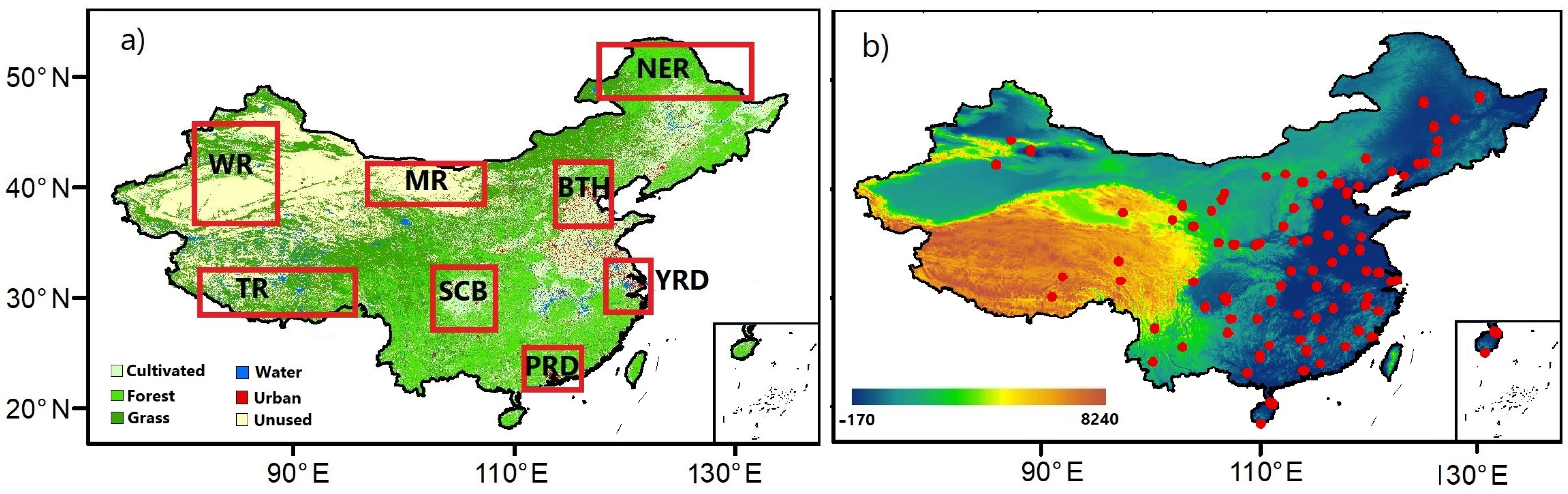
2.1. Regions of Interest

China is a global hotspot for high concentrations of aerosol particles [40,41]. In this study, eight representative regions of China were selected (Figure 1) to analyze the long-term dynamics of SO2 concentrations via satellite observations and reanalysis. The four regions of interest (ROIs) represent urban areas with high population density and loading of anthropogenic emissions [25,42]; these regions are the Yangtze River Delta (YRD, 117°E_122°E, 28°N_33°N), Beijing-Tianjin-Hebei (BTH, 113°E_119°E, 36°N_42°N), Pearl River Delta (PRD, 108°E_114°E, 20°N_26°N), and the Sichuan Basin (SCB, 103°E_108°E, 26°N_31°N) [43,44,45]. Meanwhile, the four other examined ROIs representing rural regions in this study are largely covered by forests or desert (Figure 1), and are arid areas with less population density and low GDP (Figure S1); these are the Northeast Region (NER, 118°E_129 ° E, 49 °N_53 °N), Mongolian Region (MR, 97°E_111°E, 38°N_42°N), West Region (WR, 81°E_89°E, 37°N_43°N), and Tibetan Plateau Region (TR, 80°E_98°E, 28°N_33°N) [46,47,48].

2.2. Database

2.2.1. SO2 Data

The Chinese National Environmental Monitoring Center (CNEMC) provides ground observations of SO2 concentrations. Many ground stations were established in China in 2012. In this study, 100 sites with complete ground-based SO2 concentrations data (2013–2021) were used (Figure 1) to evaluate the MERRA-2 SO2 products, based on monthly averages. The SO2 observation sites were also used in the trend analysis. Further details regarding the Chinese observational data can be found at (http://www.cnemc.cn/, accessed on 3 March 2020) (Table 1).
MERRA-2 is the second version of the atmospheric reanalysis of the modern satellite era and uses the Atmospheric Data Assimilation System (ADAS) and the Goddard Earth Observing System Model, Version 5 (GEOS-5). MERRA-2 utilizes a radiatively coupled version of the Goddard Chemistry, Aerosol, Radiation and Transport (GOCART) aerosol module [49,50,51,52] to simulate 15 externally mixed aerosol mass mixing ratio tracers, including SO2 concentrations. In this study, SO2 concentrations, based on monthly means from MERRA-2, were used for our assessment during the 1980–2021 period (Table 1). Based on the SO2 ground-based observations from 2013 to 2021, we evaluated the uncertainty of MERRA-2 SO2 products in China based on SO2 ground-based observations from 2013 to 2021. The results showed a significant overall agreement between MERRA-2 SO2 and ground-based SO2 across China, with an acceptable bias for annual mean data, and correlation coefficient of R = 0.76 [root-mean square error (RMSE): 8.3 µg m−3; mean absolute error (MAE): 8.9 µg m−3; fractional gross error (FGE): 1.39; mean fractional error (MFE): 45.3%; and relative mean bias (RMB): 1.11]. For more details on the comparison and validation processes, please refer to Text S1 and Figures S1 and S2, in the Supplementary Material.
In addition to MERRA-2, this study utilized the total column SO2 concentration over China from the CAMS model reanalysis initiated by the European Center for Medium-range Weather Forecasts (ECMWF) (https://ecmwf.int/, accessed on 15 December 2022). CAMS combines observation data assimilation and forecasting systems to analyze daily products and 5-d forecasts of atmospheric composition, including forecasts of SO2 in near real time [17,53,54]. Monthly means of the SO2 total column datasets (at 0.75° × 0.75° longitude–latitude grid of resolution) (Table 1), provided by CAMS during the period 2007–2021, were used in the current study to improve the assessment, including annual and seasonal variabilities and inter-comparisons with the MERRA-2 dataset.
The OMI sensor is onboard the Earth Observing System (EOS) Aura satellite [55]. In the spectral zoom-in measurement mode, OMI enables the retrieval of aerosols, OClO, HCHO, ozone, and particularly SO2 observations at a spatial resolution of 25 km × 13 km at the nadir [8], with near global coverage [55]. The OMI columnar SO2 is given in Dobson units (DU), with 1 DU = 2.69 × 10¹⁶ molecules·cm−2 [8,17]. The single retrieval error of SO2 was estimated to be about 70–150% [21]. However, a previous study demonstrated the validity of using OMI SO2 data in China [8]. In this study, the OMI monthly mean SO2 total column datasets from 2007 to 2021 were used from (https://disc.sci.gsfc.nasa.gov/, accessed on 15 May 2023).

2.2.2. Key Driving Factors

Driving factors associated with human activity play a key role in regional-scale SO2 changes. More specifically, population has been recognized to be one of the main factors influencing changes in anthropogenic emissions. In addition, urban-land expansion presents a critical influence on understanding changes in urban emission rates [56,57]. GDP is used to describe the economic development of a country, which in China often drives construction activities and increases fossil fuel consumption and anthropogenic emissions [58,59].
In this study, population, urbanization, and GDP were selected as the main driving factors for analyzing the dynamics of SO2 in China. Population data were taken from the Gridded Population of the World version 3 (GPWv3) from 1990 to 2000, and version 4 (GPWv4) from 2000 to 2020, provided by the NASA Socioeconomic Data and Applications Center. Both versions were at 2.5-arcminute resolution, with 5-year intervals [25], and further information related to the population are available at (http://sedac.ciesin.columbia.edu/, accessed on 15 March 2023) (Table 1). Urban-land expansion is presented as an urban area percentage, which refers to the ratio between the urban and total land areas, serving as a measure of the degree of urbanization [60].
Land-use data in the ROIs were provided by the Chinese Academy of Sciences (CAS) through the National Resources and Environment Database, including a series of five years of temporal resolution from late 1990 to 2019. There are six primary land use categories (http://www.resdc.cn/, accessed on 15 March 2023). In this study, artificial surface classes were extracted and used from 1990 to 2020 to determine the influence of urbanization. The data were highly recommended as being of high quality and have been used in previous studies [61,62].
The GDP data used in this study were provided by the CAS covering the period from 1990 to 2019. The datasets were bilinearly interpolated to a grid map using Chinese governmental data [58,63].

2.3. Trend and Regression Analysis

Trend analysis was implemented using monthly timeseries of SO2 concentrations from MERRA-2, and the total column from CAMS and OMI over the examined ROIs, using the least-squares linear regression technique, which is often used for long-term analyses [29,64]. Before the linear regression analysis, the MERRA-2, CAMS, and OMI retrievals were bilinearly interpolated to spatial grids with 1° × 1° resolution. For each grid, the annual cycle of monthly averages was removed [65,66] using annual average data. The Student’s t test was applied, and the 95% confidence level (p < 0.05) was set as the cut-off for statistical significance [67,68].
To better understand the effects of the total population (TP), GDP, and urbanization percentage (UP) on SO2 concentrations in each ROI, MERRA-2 SO2 concentrations obtained during the years 1990–2021 were averaged based on 3-year means. For example, the year 2000 value represents the average of the values in 1999, 2000, and 2001, with five-year temporal intervals. Subsequently, the averaged MERRA-2 SO2 concentrations were linked to population, urbanization, and GDP for 1990, 1995, 2000, 2005, 2010, 2015, and 2020. The strength of the relationships was measured using the Pearson correlation coefficient (R). An ordinary least squares regression model (OLS) [59,69,70,71,72] was used in this study. The OLS method is given in Equation (1)
y = β   x   + β 0 + ϵ ,
where y is the extracted mean SO2 concentration of an ROI as the dependent variable; and β x is the regression coefficient of the independent variables; for example, TP, GDP, and UP. β 0 is the value of the intercept, and ε refers to the standard error. Geographically weighted regression (GWR) models explain the spatial variation in the strength of the relationships between factors across selected geolocation regions [59,73]. Therefore, the GWR model was used in a form similar to that of the OLS model. Nevertheless, the selected parameters differ according to the geographical location. The GWR is given in Equation (2) as:
y j = β o u j , v j + i = 1 p β i u j , v j x i j + ε j
where β o u j , v j is the intercept value for position (j) at coordinates u j , v j ; and β i u j , v j is the estimated independent variable of local parameters, such as TP, GDP, and UP of (xi) at location (j). In addition to the localization of the parameters, spatial autocorrelation was accurately included in the GWR model. A defining feature of GWR is that the selected parameters are allowed to vary across spaces to measure non-static spatial relationships. Using different bandwidths and a representation of the matrix for each period, the estimated value of the selected variable can be expressed by Equation (3)
β f u j , v j = X T W u j , v j X 1 X T W u j , v j y
where T is the matrix transpose operation; β f u j , v j is the weight of the specific location of the variable; and W u j , v j is a (number) by (number) spatial weight matrix at location j. All the calculations of GWR were performed in ArcGIS software version 10.8 via a model (GTWR Beta 1.0) developed by [74,75]. To examine the relative contributions (%) of the selected variables to SO2 concentration changes, the method of Lindeman, Merenda, and Gold (LMG) [12,28,76] was used. The LMG can be calculated as.
L M G ( x i   ) = 1 p !   r   p e r m u t a t i o n       s e q R 2 ( { x i   } { r } )
the rth (r = 1, 2, …, p!) represented by r, and s e q R 2 ( { x i } { r } ) denotes the sequential of sum squares for the r of xi in the ordering of the r in the rth.

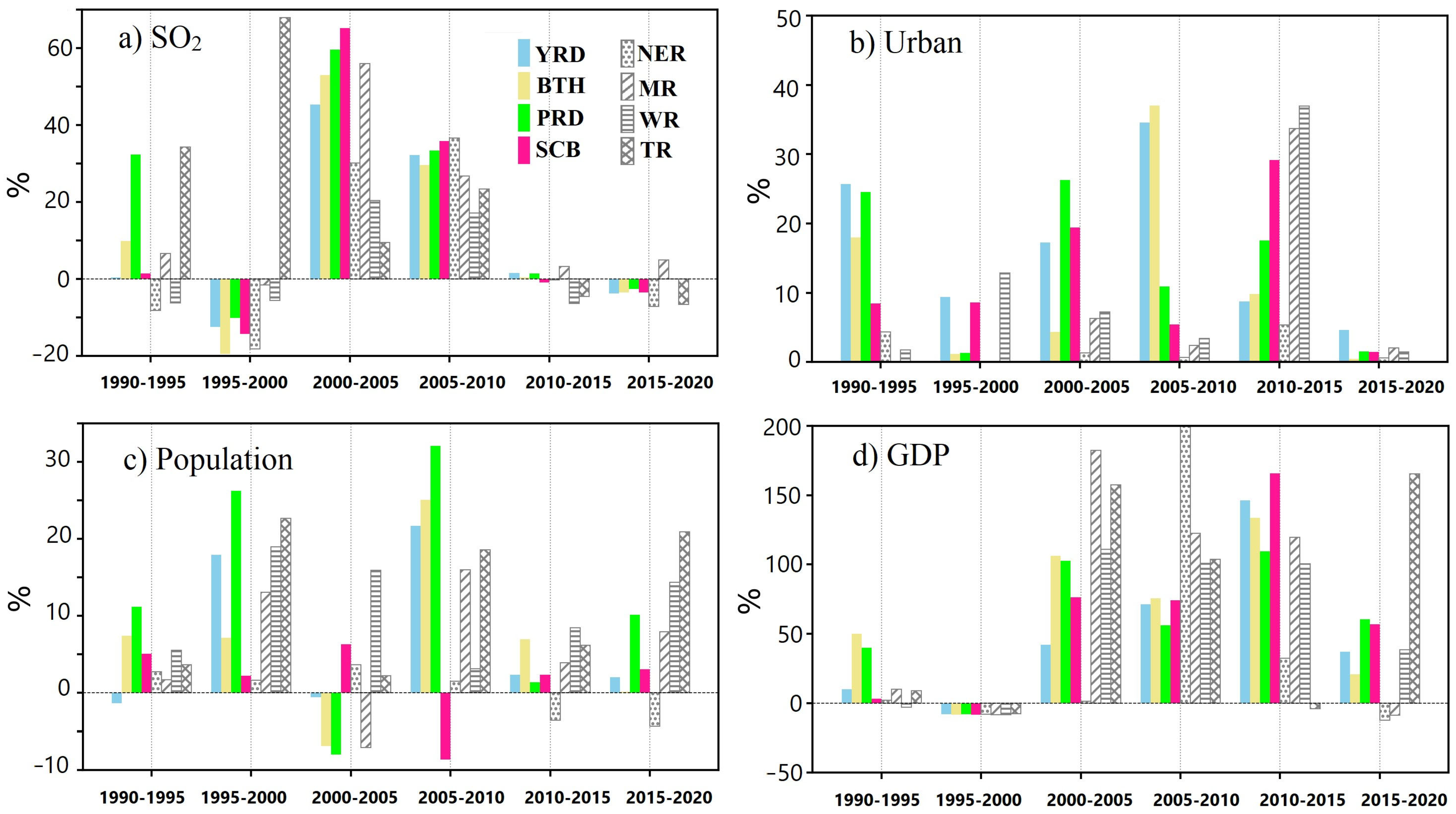
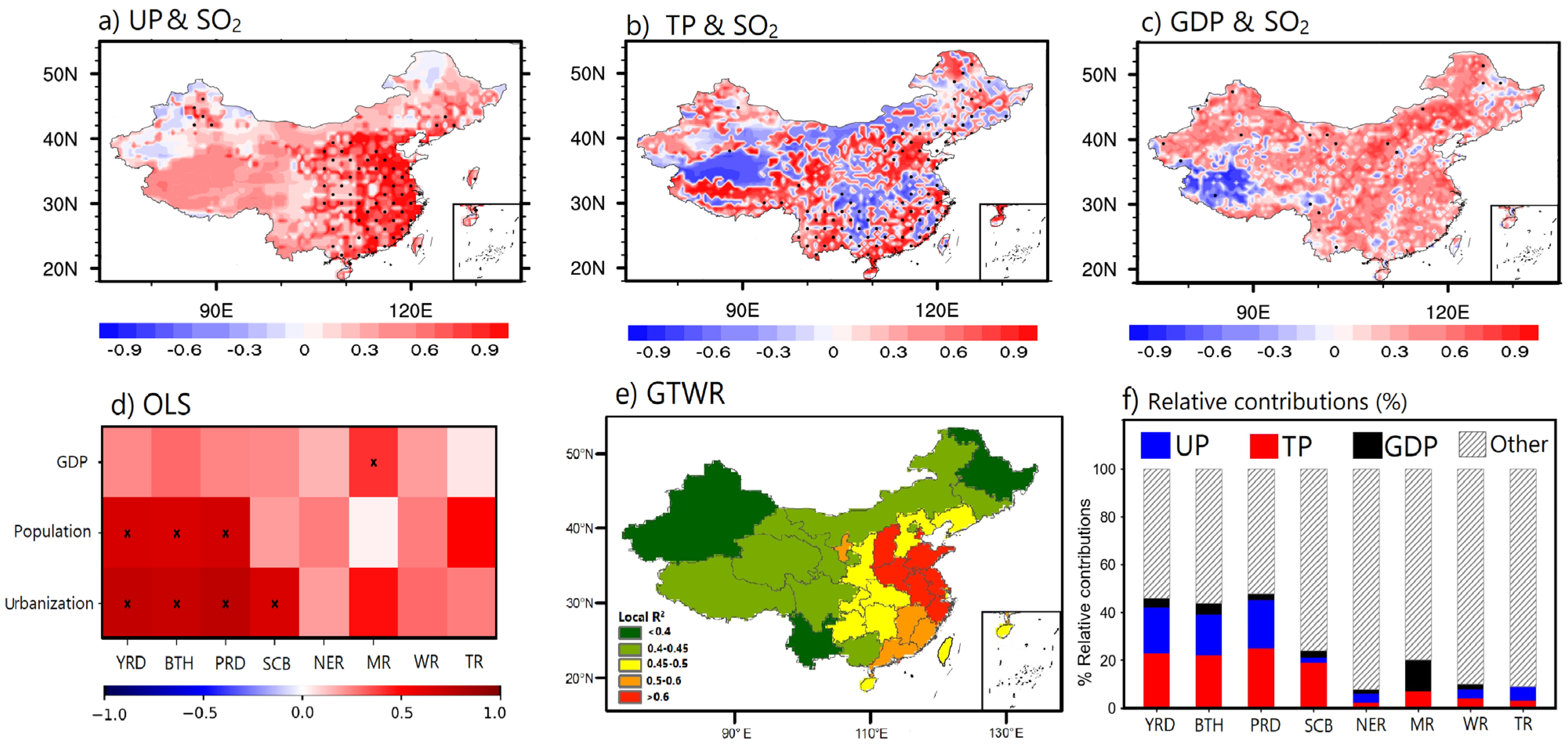
3. Results and Discussion

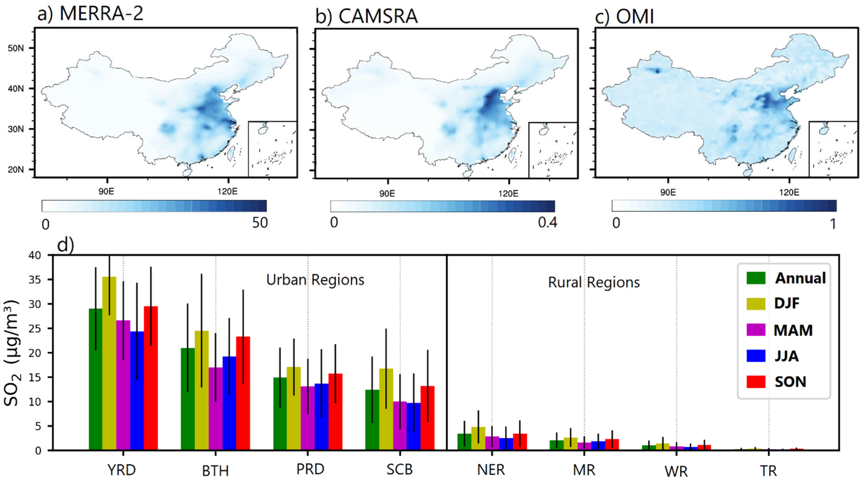
3.1. Spatial Patterns of SO2 Concentrations

Figure 2 displays the spatial patterns of the annual mean SO2 calculated from the MERRA-2, CAMS, and OMI data over China during 1980–2021, 2007–2021, and 2007–2021, respectively. The three datasets showed similar patterns of SO2 over China despite the different time periods, with the highest values observed over the Eastern China plains, near large urban agglomerations such as PRD, YRD, BTH, and SCB. Due to different units in SO2 concentrations between the three datasets, only a qualitative visualized comparison can be extracted from the spatial distribution maps (Figure 2a–c). Figure 2d shows the seasonal mean SO2 concentrations (in μg m−3) over the eight selected regions in China, as analyzed from MERRA–2 during 1980–2021.
High SO2 loading was mainly observed in the urban regions of China. The YRD and BTH regions located in eastern China are highly dominated by anthropogenic emissions [43,45,77,78] and exhibited a very high amount of SO2. In contrast, the SO2 concentrations were the lowest in the TR and WR remote areas, as expected. The multi-year average of MERRA-2 SO2 concentrations is the highest in YRD (28.9 ± 8.5 μg m−3) followed by BTH (20.9 ± 9.1 μg m−3), PRD (14.9 ± 6.1 μg m−3), and SCB (12.4 ± 6.8 μg m−3). Industrialization and urbanization play a key role in the increase in SO2 emissions in eastern China [8]. SO2 from areas of high anthropogenic and industrial emissions tends to affect the SO2 concentration distribution at a local rather than regional scale [79,80]. Over the four selected rural regions, the annual average SO2 concentrations were highest in NER (3.4 ± 2.6 μg m−3) and lowest in TR (0.26 ± 0.2 μg m−3). Note that the multi-year average of MERRA-2 SO2 concentrations over the four selected rural regions is about 11 times lower than that over the corresponding urban regions.
A comparison of the three products showed that the mean spatial distribution of the MERRA-2 SO2 concentrations agreed well with the results of CAMS and OMI in most regions of China, with relatively small differences. On a seasonal timescale, high SO2 loading was mainly observed in winter (December, January, and February; DJF) and autumn (September, October, and November; SON), whereas the concentration of MERRA–2 SO2 was relatively low in spring (March, April, and May; MAM) and summer (June, July, and August; JJA) (Figure 3). Previous studies have shown that approximately 35% of the annual average of SO2 concentrations over East China occur during the winter, whereas the summer season contributes only 15% to the annual SO2 loading [24]. Previous study [8] also reported highest SO2 concentrations in winter in China from 2013 to 2016.
The current results of the highest seasonal mean SO2 distribution in winter, followed by autumn, were also similar among the three SO2 datasets (Figure 3). Particulate matter (PM), including sulfate aerosols produced by human activities in winter and autumn, is the main contributor to high aerosol loading in eastern China [81]. The higher concentrations of SO2 in autumn and winter can be attributed mainly to the increased demand for coal consumption, resulting in an increase in SO2 loading along with increased black carbon, NOx and organic aerosols [8,27,31,37]. Moreover, lower humidity and cold temperatures, attributed to the winter East Asian monsoon, jointly weaken wet deposition and oxidation rates, extending the lifetime of SO2 molecules [24], thus favoring the SO2 accumulation. SO2 loading is relatively low in spring and summer because of seasonal variations in atmospheric turbulence driven by solar radiation, which makes wet removal effective during the monsoon period [12,82,83].

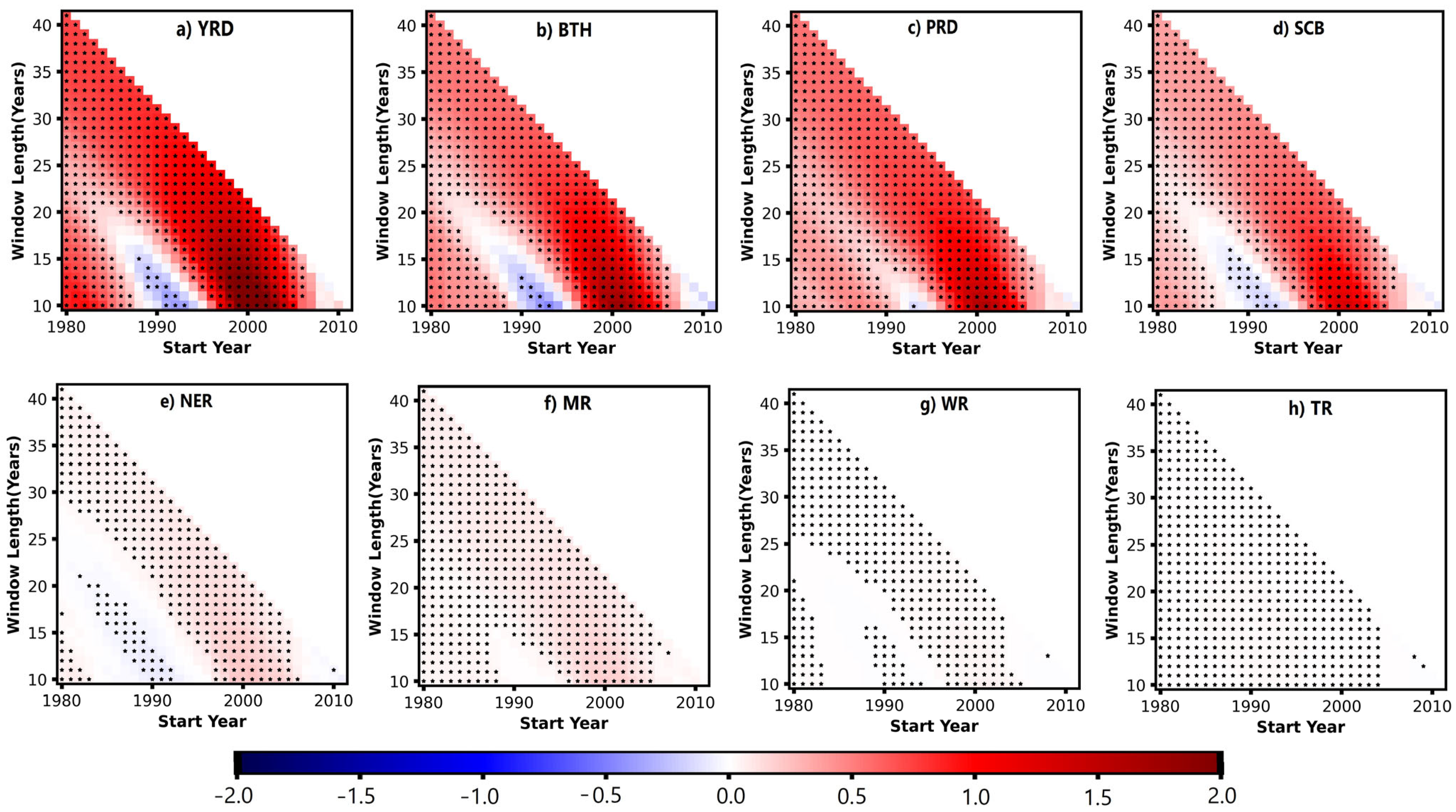
3.2. Trends in SO2 Concentrations

To better assess the temporal variation and trends of MERRA-2 SO2 concentrations, normalized annual anomalies were examined during the period 1980–2021 over the selected urban (YRD, BTH, PRD, and SCB) and rural (NER, MR, WR, and TR) regions (Figure 4). The results show that SO2 concentrations have experienced relatively similar and significant (p < 0.05) positive trends in both urban and rural regions during 1980–2021. Significant increasing trends were observed in YRD (0.71 µg m−3 yr−1), BTH (0.5 µg m−3 yr−1), PRD (0.52 µg m−3 yr−1), and SCB (0.35 µg m−3 yr−1). The percentage of relative change in SO2 concentrations between 1980 and 2021 exceeded 100% over the selected urban regions (Table 2), with the highest percentage increase (232%) detected in PRD. Over the four selected rural regions, statistically significant, but weaker, increasing trends were observed during 1980–2021 with rates of 0.04 µg m−3 yr−1 in MER, 0.06 µg m−3 yr−1 in MR, 0.01 µg m−3 yr−1 in WR, and 0.012 µg m−3 yr−1 in TR (Figure 4).
However, the relative change in SO2 concentrations in TR was particularly high (256%) from 1980 to 2021 (Table 2), likely due to low SO2 concentrations in this remote region. Notably, the average of the increasing trends of MERRA-2 SO2 over the four urban regions was approximately 16 times higher than the average SO2 trends over the four rural regions, which is attributed to rapid economic growth, increase in energy consumption, and anthropogenic emissions in urban compared to rural regions [12,26,35]. For a more precise investigation of the long-term temporal changes in SO2 concentrations, sliding trend analyses were applied to calculate the annual trends over urban and rural regions during different periods from 1980 to 2011 using spans of 10 years. As shown in Figure 5, the MERRA-2 SO2 concentrations showed different trends throughout the study period. Therefore, the long-term variations and trends in SO2 can be divided into three sub-periods: 1980–1997, 1997–2001, and 2001–2010.
From 1980 to 1997, MERRA-2 SO2 concentrations increased over the four selected urban regions (Table 2) at rates of 0.57 µg m−3 yr−1 in YRD, 0.44 µg m−3 yr−1 in BTH, 0.37 µg m−3 yr−1 in PRD, and 0.22 µg m−3 yr−1 in SCB. Furthermore, it is worth noting that the SO2 levels over the unpolluted and economically underdeveloped regions were also raised during 1980–1997, as SO2 concentrations significantly increased over the four selected rural regions of China at rates of 0.01, 0.03, 0.007, and 0.008 µg m−3 yr−1 over NER, MR, WR, and TR regions, respectively (Table 2). Previous studies showed an annual growth rate of 3.0–6.8% of SO2 emissions over China during the periods before 1995 [12,13,26,35,84]. The overall increase in SO2 over China during 1980–1997 (Figure 6) could be mainly attributed to the rapid growth of fossil fuel and coal consumption [35] due to increasing energy demands, especially in Eastern China (Figure 6). In addition, the percentage of vehicular emissions increased due to population and GDP growth until 1995 [26], which also enhanced SO2 emissions, as shown below.
During 1997–2001, MERRA-2 SO2 showed significant negative trends over eastern China (Figure 6). During this period, MERRA-2 SO2 concentrations decreased by 25%, 28%, 11%, and 18% in YRD, BTH, PRD, and SCB, respectively. Over the rural regions, SO2 concentrations also showed significant decreasing trends in NER (−0.1 µg m−3 yr−1), WR (−0.01 µg m−3 yr−1), and TR (−0.03 µg m−3 yr−1). However, SO2 concentrations presented a slight increasing trend in the TR at a rate of 0.03 µg m−3 yr−1. The decreasing SO2 concentrations over a large part of China during 1997–2001 could be mainly attributed to the Asian economic crisis, which started in 1997 with a decrease in GDP [85] (see also the following section), and then a decrease in energy consumption. Similar decreasing trends in industrial emissions and SO2 concentrations were also observed over southern Europe, mainly in Greece, after the 2008 crisis and the subsequent economic recession [86]. In contrast, after 2001, the SO2 concentrations increased significantly in all regions of China (Figure 6). Previous studies also noted that the SO2 emissions increased by approximately 5–7% annually over China during 2001–2006 [87,88]. Our trend analysis showed that MERRA-2 SO2 concentrations increased rapidly over the four selected urban regions at rates of 2.42, 1.68, 1.52 and 1.23 µg m−3 yr−1 in YRD, BTH, PRD, and SCB, respectively. Moreover, SO2 concentrations also showed significantly increasing trends over the selected rural regions at rates of 0.21, 0.16, 0.04, and 0.014 µg m−3 yr−1 in NER, MR, WR, and TR, respectively.
The relative changes showed that the average SO2 concentration trends were approximately 16 times higher over the four urban regions than in the corresponding rural regions during 2001–2010. This dramatic increase in SO2 concentrations over the urban regions of China is mainly associated with rapid urbanization, increase in China’s economy, and large fuel consumption to meet increasing energy demands [26].
In contrast, the MERRA-2 SO2 concentrations decreased slightly over China during the last decade (Figure 5), which is also shown for the period 2007–2021 (Figure 6). Several studies have shown that SO2 emissions began to decline significantly after 2006, thereby improving air quality [26,28]. To better understand the changes in SO2 emissions, CAMS and OMI data were also used, which were in general agreement with the MERRA-2 SO2 variations, indicating downward trends in most parts of Eastern China (Figure 6). More specifically, the total column of SO2 from CAMS data showed significant negative trends over the examined urban area, with rates of −0.15, −0.05, and −0.06 mg m−2 yr−1 in YRD, PRD, and SCB, respectively. SO2 columns from the OMI sensors also showed significant negative trends over large areas close to the urban agglomerations of China with rates of −0.024, −0.03, and −0.02 DU yr−1 in YRD, BTH, and SCB, respectively. Similar to a previous study of the impact of the Chinese Five-Year Plans (FYPs) on anthropogenic aerosols over China [28,89], our study suggests decreasing trends in SO2 concentrations over most parts of eastern China in response to FYPs. Further details regarding the impact of FYPs on SO2 concentrations are provided in Section 3.4. Over the four selected rural regions of China, MERRA-2, CAMS, and OMI showed insignificant trends during 2007–2021, except for NER, where CAMS showed a significant decreasing trend at a rate of 0.04 mg m−2 yr−1. However, there were some differences in the trends between MERRA-2, CAMS, and OMI data in some parts of China during the years 2007–2021, which were mainly attributed to the different databases, retrieval algorithms, and reanalysis data. In [17], the authors also noted differences in trend directions of SO2 concentrations over India using MERRA-2, CAMS, and OMI data. Such differences could be attributed to missing satellite data and different assimilation algorithms used in the reanalysis data [17,90,91].

3.3. The Impact of Driving Factors on SO2

To understand the influences of TP, GDP, and UP on SO2 concentrations in each region, five years of relative changes in SO2, UP, TP, and GDP in the eight ROIs during 1990–2020 were investigated (Figure 5). Relative changes in MERRA-2 SO2 during 1990–1995 showed an obvious increase in SO2 concentrations in BTH, PRD, MR, and TR, while SO2 concentrations remained approximately stable over YRD and SCB and decreased in NER and WR (Figure 7). During the same period, UPs largely increased over the four selected urban regions compared to the rural regions (Figure 7). The TP data suggested an increase from 1990 to 1995 over all regions, except for YRD. GDP increased by approximately 50% and 40% in PRD and BTH, respectively, in the selected period and increased slightly to moderately over the other regions. Overall, the relationship between the changes in SO2 and human activity factors could not be easily determined. For example, the most populated region of China, YRD, exhibited a negligible change in SO2 concentrations during 1990–1995, corresponding to an approximately 25% relative increase in urban percentage, an approximately 10% increase in GDP, and a slight decrease in total population.
During the years 1995–2000, MERRA-2 SO2 concentrations showed a notable decrease over all the selected regions except for TR, which was highly linked with an average decrease of 7–8% in Chinese GDP. In contrast, the UP and TP data showed increases in the selected regions during 1995–2000. Furthermore, during 2000–2005 and 2005–2010, SO2 concentrations increased over all ROIs, which was in good agreement with the increase in UP and GDP in the eight ROIs during the same periods. However, TP data showed an average 5% decrease in relative changes in BTH and PRD during 2000–2005, and a 7% decrease in relative changes in the SCB during 2005–2010. During the last two periods, 2010–2015 and 2015–2020, the MERRA-2 SO2 concentrations exhibited negligible changes or even slight decreases. However, these changes in SO2 were not in good agreement with those of human factors because UP, TP, and GDP showed increasing tendencies over the different ROIs during 2010–2015 and 2015–2020, thus highlighting the effect of the clean-air policies followed in China during the last decade.
To better understand the changes in SO2 concentrations with respect to human activity factors, a regression model was applied to China and the eight ROIs; the results are presented in Figure 8. A significant (p < 0.05) positive correlation between UP and SO2 was observed in Central and Eastern China (Figure 8), which are regions highly dominated by urban areas. However, nonsignificant positive correlations between UP and SO2 were found in Northern, Western, and Southern China, which are mostly rural areas. Our results showed that the UP in the four selected urban regions (YRD, BTH, PRD, and SCB) was positively correlated (p < 0.05) with SO2, suggesting that the UP could be a major factor controlling SO2 variations. Previous studies have suggested that the increase in PM2.5 concentrations over the urban regions of China is directly linked to the increase and expansion of urban areas [28,92]. Another factor that could affect SO2 variation in China is the total population. Our statistical results suggest a significant positive correlation between TP and SO2 over some urban areas in China with large populations. Therefore, TP in the three selected urban regions (YRD, BTH, and PRD) was positively (p < 0.05) correlated with SO2, indicating that TP could be another factor controlling SO2 variations in the selected regions. In the SCB, TP was not significantly correlated with SO2, which could be attributed to the decrease in TP during a period of high increase in SO2 emissions, i.e., from 2005 to 2010. Our results showed nonsignificant (p < 0.05) positive correlations between SO2 concentrations and TP in rural regions (NER, MR, WR, and TR). This leads to the conclusion that the UP and TP may not play a significant role in SO2 variation in the rural regions of China. In addition, GDP was positively correlated with SO2 over vast areas of China. However, a significant correlation was found only in the MR. This finding was consistent with previous studies that suggested positive correlations between GDP, internal migration, and air pollutants in China [92,93].
The influence of the human factors was further tested using the GTWR model. The three variables (UP, TP, and GDP) were assimilated into the GTWR model under the conditions of Akaike Information Criterion (AIC) minimization and non-collinearity. Figure 8e shows the determination coefficients (R2) for provincial areas obtained from the GTWR model. The spatial distribution of the R2 values revealed the combined effects of UP, TP, and GDP on SO2 concentrations. The R2 varied from 0.36 to 0.75 across China, with the highest values in the urban/populated provinces in eastern China, compared to the rural and remote regions in NW, NE, central China, and the TR (Figure 8e). This reveals that the UP, TP, and GDP seem to have a stronger influence on SO2 variations in urban regions than in rural ones in China.
The contribution of each factor (UP, TP, and GDP) on SO2 concentration changes was also investigated. Our analysis showed that the UP is a dominant human activity-driving factor that contributes to SO2 concentration changes of about 23.3%, 22.2%, 25.4%, and 19.3% in YRD, BTH, PRD, and SCB, respectively (Figure 8f). Previous studies suggested that the urban class was a dominant factor in PM2.5 changes in east and south China [28,61]. Over YRD, BTH, PRD, and SCB explains about 19.1%, 17.3%, 20.2%, and 7.9% of the changes of SO2 concentrations, respectively (Figure 8f). Furthermore, over the urban regions, the GDP exhibited low and insignificant contributions (3–5%) to SO2 changes, while over the rural regions, the UP and TP contributed less (0.5–6%) to SO2 variations (Figure 8f). GDP data contributed about 13% to SO2 changes over the MR region. Previous studies have suggested that human activity factors, including urbanization, have nonsignificantly contributed to PM2.5 changes in the rural regions of China [28,61]. On the other hand, meteorological variables are believed to have significant influence on PM2.5 decadal changes [76,94], thus weakening the role of the population density, expansion of urban areas, and GDP [61,95]. It is worth mentioning that despite the continuous increase in population, GDP, and urban areas that potentially enhance air pollution, the SO2 concentrations displayed a declining trend after the year 2010 over large regions in China. The decrease in SO2 levels could be attributed to the effects of Chinese policies to control air pollution and other clean-air mitigation strategies, which are addressed below.

3.4. The Role of Chinese Government Policies

A series of air pollution prevention and control policies has been implemented in China over the last two decades. The 11th (2006–2010), 12th (2011–2015) and 13th (2016–2020) FYPs have been applied [28,89]. These plans were intended to improve the air quality in Chinese megacities and surrounding areas by reducing anthropogenic emissions.
To better evaluate the temporal changes in SO2 in response to Chinese emissions control policies, a trend analysis was applied over the selected urban and rural regions using SO2 concentration data from MERRA-2, CAMS, and OMI during the periods 2006–2010, 2011–2015, and 2016–2021 (Table 3). In general, the 11th FYP was planned to reduce the SO2 concentrations by 10% during 2006–2010 [28,89]. Throughout the 11th FYP, MERRA-2 SO2 showed nonsignificant positive trends over both the examined urban and rural regions, except for NER where the trend (0.23 µg m−3 yr−1) was statistically significant. A previous study also showed that the AOD and PM2.5 concentrations from MERRA-2 data did not sufficiently decrease in response to the 11th FYP [28,96].
In comparison, CAMS and OMI SO2 showed negative trends in the four selected urban areas with significant declining trends of −0.45 and −0.65 mg m−2. yr−1 in YRD and BTH, respectively, and −0.08 DU yr−1 in BTH, thus coinciding with the implementation of the plans. In response to the 11th FYP, CAMS and OMI SO2 levels revealed a reduction range of 2–45% over the four examined urban regions during 2006–2010. SO2 concentrations began to decrease in 2006, which was mainly attributed to the application of flue gas desulfurization in Chinese power plants [97,98]. In addition, the rural regions exhibited negative trends in CAMS and OMI SO2 data, with significant declining rates of −0.06 mg m−2 yr−1 and −0.023 DU yr−1 for CAMS and OMI in MR, respectively (Figure 9a). These reductions in rural regions could be mainly associated with a general reduction in urban/industrial SO2 emissions from the main sources in East China.
During the 12th FYP, the ratio of energy consumption to per-capita GDP was planned to decrease by 16% and SO2 concentrations were to be reduced by 8–10%. During the 12th FYP implementation period (2011–2015), MERRA-2 SO2 concentrations began to exhibit negative trends over urban regions, except for the YRD. In the four rural regions, negative MERRA-2 SO2 trends were also observed (Figure 9b). CAMS SO2 also showed decreasing trends in YRD and PRD, whereas BTH exhibited an increasing trend. Furthermore, over the urban regions of YRD and BTH, OMI SO2 concentrations showed a decreasing trend. Nonetheless, SO2 increased slightly in the PRD during the same period. In 2011–2015 (12th FYP), CAMS and OMI SO2 concentrations showed significant decreasing trends in SCB with rates of −0.26 mg m−2 yr−1 and −0.03 DU yr−1, respectively. SO2 reductions were also noted over the rural regions of China using CAMS and OMI data, which could be mainly attributed to SO2 reduction from sources in Chinese urban regions.
A 15% reduction in SO2 by 2020 compared to 2015 levels was planned through the 13th FYP. During 2016–2021, the three datasets showed consistent negative SO2 trends over the urban regions (Figure 9c), with significant decreasing trends in SCB for MERRA-2 (−0.95 µg m−3 yr−1) and OMI (−0.03 DU yr−1). Overall, MERRA-2, CAMS, and OMI SO2 data revealed a reduction range of 3–30% from 2016 to 2021 over the four urban regions. In the four rural regions, negative trends were also observed during the same period in the three datasets, except for in NER and WR, as OMI showed increasing trends of 0.01 and 0.002 DU yr−1, respectively.
Because there were no ground measurements in 2012, 2013 was used as the primary year to evaluate the achievement of the 12th and 13th FYPs. Furthermore, the 12th and 13th FYPs largely focused on reducing SO2 levels via desulfurization in the industrial and traffic sectors [28,96,99]. Thus, a trend examination was applied to SO2 from the CAMS, OMI, MERRA-2, and ground stations in the years 2013–2021 (Figure 9). The results indicate that SO2 concentrations from MERRA-2 declined over eastern China and in the four urban regions. However, the distribution of the trends was more variable for the CAMS data, which showed increasing trends in the YRD and PRD regions and a significant decreasing trend in the SCB at a rate of −0.13 mg m−2 yr−1. In contrast, OMI also exhibited a large spatial variation in trend values, with significant decreasing trends in the three urban regions, except for the PRD (Figure 9g). Similar significant decreasing trends in SO2 concentrations were also observed at the ground monitoring stations during 2013–2021, which were mostly detected in Eastern China but also in the northeast, central, and northwest regions, as well as in the TR and southern rural areas. Therefore, the implementation of FYPs since 2007 has led to a significant drop in SO2 concentrations during the last decade in China, not only in urban/industrialized regions but also in rural and remote areas. Consistent with several previous studies [26,28,95], the FYPs reduced SO2 concentrations (among other air pollutants) and improved air quality.

4. Conclusions

In this study, we assessed the long-term trends in SO2 concentrations over China from 1980 to 2021 based on reanalysis data (MERRA-2). We also examined the SO2 total column using data from CAMS reanalysis and OMI satellite observations from 2007 to 2021. Eight representative regions, including four urban (PRD, BTH, YRD, and SCB) and four rural (NER, MR, WR, and TR), were selected for analysis. The relationships between SO2 multi-year variations and influencing factors, including GDP, population, and urbanization, were explored using linear regression and geographical temporally weighted regression models to evaluate the anthropogenic impacts on SO2 concentrations. Finally, we examined the influence of control policies on SO2 trends after 2006. The main findings of this study are summarized as follows:
  • The multi-year average SO2 concentrations from MERRA-2 data from 1980 to 2021 over the four rural regions are approximately 11 times lower than those over the four urban regions.
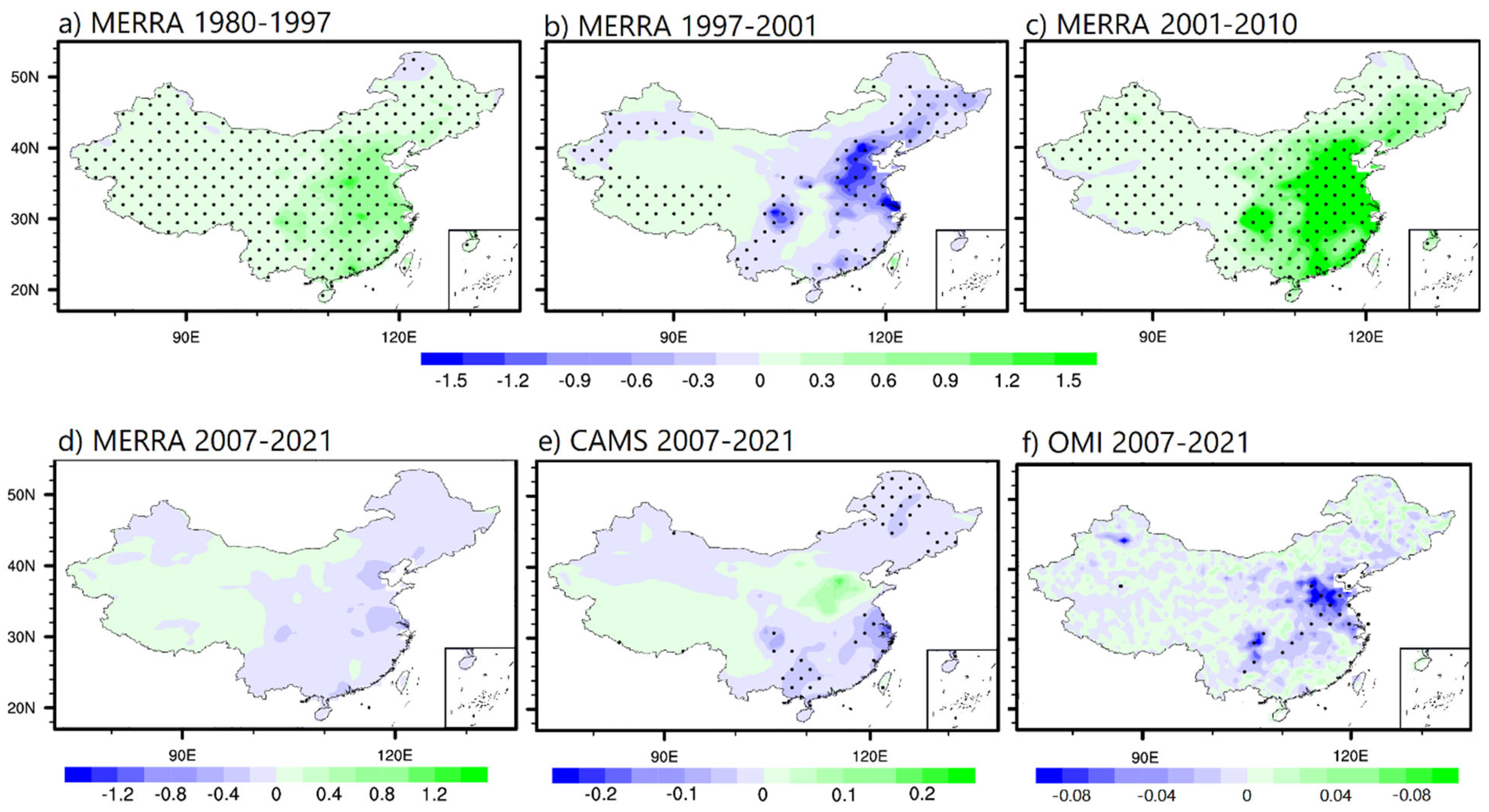
  • The SO2 concentration increased significantly over the selected regions from 1980 to 2021, with major changes occurring in between. It increased during 1980–1997 and 2001–2010, but dropped during 1997–2001 and 2010–2021. The relative change showed that the average MERRA-2 SO2 concentration trends over the four urban regions were approximately 16 times higher than those in the four rural regions.
  • The results revealed that the driving factors associated with human activities, including urbanization, GDP, and population, played significant roles in multi-decadal SO2 variations and trends in the main urban areas of China.
  • The SO2 concentration significantly decreased in most regions of China after 2010, which was attributed to the control policies of China (12th and 13th FYP).
  • The OMI SO2 data showed significant downward trends in the last decade over most regions of China, exhibiting better agreement with SO2 variations from ground-based stations than with SO2 data from the MERRA-2 and CAMS reanalysis.
The assessment of the long-term dynamics of SO2 concentrations revealed that variations in SO2 concentrations were highly influenced by human activities in the urban areas of China. Nonetheless, with continued anthropogenic activities associated with urban expansion, SO2 levels showed a declining trend after 2007, which is credited to the control policies of China. Our project improves our understanding of the long-term changes in SO2 concentrations in urban regions of China compared to rural regions, as well as the effects of mitigation strategies and air pollution control plans.

5. Limitations and Future Prospects

This study used different SO2 datasets, including observation data from OMI, and reanalysis data from MERRA-2 and CAMS. For the OMI satellite data, the primary sources of uncertainty were mainly associated with haze and cloud condensation. In addition, some gaps were presented, which may cause some uncertainties in SO2 retrievals from satellite. On the other hand, MERRA-2 and CAMS assimilate different sources of AOD in Earth system modeling. The differences across the datasets are probably attributable to the algorithms used. Different algorithms may produce some uncertainties. Regardless of the limitation, this study would be of major interest, especially over the Chinese regions, and it comprises important information that could be of use to climate change, air quality, human activities and health in China [100,101]. Therefore, our findings highlight the importance of future studies on the impact of SO2 on regional climate change in China.

Supplementary Materials

The following supporting information can be downloaded at: https://www.mdpi.com/article/10.3390/rs16020391/s1, Figure S1: The 2020 GDP (million Chinese yuan) and the 2020 population (millions) at the province level; Text S1: Evaluation of MERRA-2 SO2 product in China; Figure S2: Comparison of the yearly SO2 concentration data obtained from MERRA-2 and ground-based monitoring stations in China; Figure S3: Comparison of yearly MERRA-2 SO2 data with SO2 measurements from 100 sites in China.

Author Contributions

Methodology, F.W., A.S., R.Y., D.G.K. and Y.Z. (Yuyu Zhou); investigation, F.W., A.S., R.Y. and D.G.K.; writing—original draft preparation, F.W., A.S., R.Y., D.G.K. and Y.Z. (Yuyu Zhou); writing—review and editing, F.W., A.S., Q.G, R.W., J.L., Z.L., Y.Z. (Yu Zhan) and Y.Z. (Yuyu Zhou); data curation, F.W., A.S., Q.G. and D.G.K.; visualization, F.W and A.S. All authors have read and agreed to the published version of the manuscript.

Funding

This project is funded by Research Project of Ministry of Science and Technology of China (2023YFF0806004).

Data Availability Statement

The 100 ground observations of SO2 concentrations for 2013-618 2021 used in the study are available at https://www.aqistudy.cn/historydata/, accessed on 15 May 2023. A request for permission from the administrative section is necessary for access. SO2 concentration data from MERRA-2 during the 1980–2021 used in the study are available at https://disc.gsfc.nasa.gov/datasets/M2TMNXAER_5.12.4/summary, accessed on 15 May 2023, and SO2 total column data from OMI during 2007–2021 used in the study are available at https://disc.gsfc.nasa.gov/datasets/OMSO2e_003/summary, accessed on 15 May 2023. SO2 total column data from CAMS during 2007–2021 used in the study are available at the Atmosphere Data Store https://ads.atmosphere.copernicus.eu/cdsapp#!/dataset/cams-global-reanalysis-eac4-monthly?tab=form, accessed on 15 May 2023. Registration is free to obtain access to the MERRA-, OMI, and CAMS data. Population data used in the current study from the Gridded Population of the World version3 (GPWv3) from 1990 to 2000 and version 4 (GPWv4) from 2000 to 2020 are free to access at https://sedac.ciesin.columbia.edu/data/set/wacvm-gpw-v4-population-density-pre-release-1-2010/data-download, accessed on 15 March 2023. LULC data from 1990 to 2020 used in the study were obtained from the Resource and Environmental Science and Data Center at https://www.resdc.cn/DOI/DOI.aspx?DOIID=54, accessed on 15 March 2023. GDP data used in the study were also obtained from Resource and Environmental Science and Data Center at https://www.resdc.cn/DOI/DOI.aspx?DOIID=33, accessed on 15 March 2023, and a permission request to the center is necessary to receive the data.

Acknowledgments

We thank the Center for Environmental Prediction (NCEP), the Earth Observing System Data and Information System (EOSDIS, NASA), the European Centre for Medium-Range Weather Forecasts (ECMWF), and the Ministry of Ecology and Environment of the People’s Republic of China.

Conflicts of Interest

The authors declare no conflicts of interest.

References

  1. Steinfeld, J.I. Atmospheric Chemistry and Physics: From Air Pollution to Climate Change; John Wiley & Sons: Hoboken, NJ, USA, 1998; Volume 40, ISBN 1118947401. [Google Scholar]
  2. Rawat, P.; Sarkar, S.; Jia, S.; Khillare, P.S.; Sharma, B. Regional Sulfate Drives Long-Term Rise in AOD over Megacity Kolkata, India. Atmos. Environ. 2019, 209, 167–181. [Google Scholar] [CrossRef]
  3. Liu, J.; Liang, D.; Liu, L.; Ning, A.; Zhang, X. Catalytic Sulfate Formation Mechanism Influenced by Important Constituents of Cloud Water via the Reaction of SO2 oxidized by Hypobromic Acid in Marine Areas. Phys. Chem. Chem. Phys. 2021, 23, 15935–15949. [Google Scholar] [CrossRef] [PubMed]
  4. Liu, J.; Ning, A.; Liu, L.; Wang, H.; Kurtén, T.; Zhang, X. A PH Dependent Sulfate Formation Mechanism Caused by Hypochlorous Acid in the Marine Atmosphere. Sci. Total Environ. 2021, 787, 147551. [Google Scholar] [CrossRef] [PubMed]
  5. Lu, Z.; Streets, D.G.; De Foy, B.; Krotkov, N.A. Ozone Monitoring Instrument Observations of Interannual Increases in SO2 Emissions from Indian Coal-Fired Power Plants during 2005–2012. Environ. Sci. Technol. 2013, 47, 13993–14000. [Google Scholar] [CrossRef]
  6. Lee, C.Y.; Zhou, P. Directional Shadow Price Estimation of CO2, SO2 and NOx in the United States Coal Power Industry 1990–2010. Energy Econ. 2015, 51, 493–502. [Google Scholar] [CrossRef]
  7. Lelieveld, J.; Evans, J.S.; Fnais, M.; Giannadaki, D.; Pozzer, A. The Contribution of Outdoor Air Pollution Sources to Premature Mortality on a Global Scale. Nature 2015, 525, 367–371. [Google Scholar] [CrossRef] [PubMed]
  8. Zhang, H.; Di, B.; Liu, D.; Li, J.; Zhan, Y. Spatiotemporal Distributions of Ambient SO2 across China Based on Satellite Retrievals and Ground Observations: Substantial Decrease in Human Exposure during 2013–2016. Environ. Res. 2019, 179, 108795. [Google Scholar] [CrossRef] [PubMed]
  9. Lelieveld, J.; Klingmüller, K.; Pozzer, A.; Burnett, R.T.; Haines, A.; Ramanathan, V. Effects of Fossil Fuel and Total Anthropogenic Emission Removal on Public Health and Climate. Proc. Natl. Acad. Sci. USA 2019, 116, 7192–7197. [Google Scholar] [CrossRef] [PubMed]
  10. Grivas, G.; Cheristanidis, S.; Chaloulakou, A.; Koutrakis, P.; Mihalopoulos, N. Elemental Composition and Source Apportionment of Fine and Coarse Particles at Traffic and Urban Background Locations in Athens, Greece. Aerosol Air Qual. Res. 2018, 18, 1642–1659. [Google Scholar] [CrossRef]
  11. Kato, N.; Akimoto, H. Anthropogenic Emissions of SO2 and NOx in Asia: Emission Inventories. Atmos. Environ. Part A Gen. Top. 1992, 26, 2997–3017. [Google Scholar] [CrossRef]
  12. Che, H.; Gui, K.; Xia, X.; Wang, Y.; Holben, B.N.; Goloub, P.; Cuevas-Agulló, E.; Wang, H.; Zheng, Y.; Zhao, H.; et al. Large Contribution of Meteorological Factors to Inter-Decadal Changes in Regional Aerosol Optical Depth. Atmos. Chem. Phys. 2019, 19, 10497–10523. [Google Scholar] [CrossRef]
  13. Smith, S.J.; van Aardenne, J.; Klimont, Z.; Andres, R.J.; Volke, A.; Delgado Arias, S. Anthropogenic Sulfur Dioxide Emissions: 1850–2005. Atmos. Chem. Phys. 2011, 11, 1101–1116. [Google Scholar] [CrossRef]
  14. Kalita, G.; Kunchala, R.K.; Fadnavis, S.; Kaskaoutis, D.G. Long Term Variability of Carbonaceous Aerosols over Southeast Asia via Reanalysis: Association with Changes in Vegetation Cover and Biomass Burning. Atmos. Res. 2020, 245, 105064. [Google Scholar] [CrossRef]
  15. Larssen, T.; Lydersen, E.; Tang, D. Acid Rain in China. Rapid Industrialization Has Put Citizens and Ecosystems at Risk. Environ. Sci. Technol. 2006, 40, 418–425. [Google Scholar] [CrossRef]
  16. Chang, C.-T.; Yang, C.-J.; Huang, K.-H.; Huang, J.-C.; Lin, T.-C. Changes of Precipitation Acidity Related to Sulfur and Nitrogen Deposition in Forests across Three Continents in North Hemisphere over Last Two Decades. Sci. Total Environ. 2022, 806, 150552. [Google Scholar] [CrossRef]
  17. Chutia, L.; Ojha, N.; Girach, I.; Pathak, B.; Sahu, L.K.; Sarangi, C.; Flemming, J.; da Silva, A.; Bhuyan, P.K. Trends in Sulfur Dioxide over the Indian Subcontinent during 2003–2019. Atmos. Environ. 2022, 284, 119189. [Google Scholar] [CrossRef]
  18. Streets, D.G.; Tsai, N.Y.; Akimoto, H.; Oka, K. Sulfur Dioxide Emissions in Asia in the Period 1985–1997. Atmos. Environ. 2000, 34, 4413–4424. [Google Scholar] [CrossRef]
  19. Stavroulas, I.; Bougiatioti, A.; Grivas, G.; Paraskevopoulou, D.; Tsagkaraki, M.; Zarmpas, P.; Liakakou, E.; Gerasopoulos, E.; Mihalopoulos, N. Sources and Processes That Control the Submicron Organic Aerosol Composition in an Urban Mediterranean Environment (Athens): A High Temporal-Resolution Chemical Composition Measurement Study. Atmos. Chem. Phys. 2019, 19, 901–919. [Google Scholar] [CrossRef]
  20. Arub, Z.; Bhandari, S.; Gani, S.; Apte, J.S.; Hildebrandt Ruiz, L.; Habib, G. Air Mass Physiochemical Characteristics over New Delhi: Impacts on Aerosol Hygroscopicity and Cloud Condensation Nuclei (CCN) Formation. Atmos. Chem. Phys. 2020, 20, 6953–6971. [Google Scholar] [CrossRef]
  21. Krotkov, N.A.; McLinden, C.A.; Li, C.; Lamsal, L.N.; Celarier, E.A.; Marchenko, S.V.; Swartz, W.H.; Bucsela, E.J.; Joiner, J.; Duncan, B.N.; et al. Aura OMI Observations of Regional SO2 and NO2 Pollution Changes from 2005 to 2015. Atmos. Chem. Phys. 2016, 16, 4605–4629. [Google Scholar] [CrossRef]
  22. Fadnavis, S.; Müller, R.; Kalita, G.; Rowlinson, M.; Rap, A.; Li, J.-L.F.; Gasparini, B.; Laakso, A. The Impact of Recent Changes in Asian Anthropogenic Emissions of SO2 on Sulfate Loading in the Upper Troposphere and Lower Stratosphere and the Associated Radiative Changes. Atmos. Chem. Phys. 2019, 19, 9989–10008. [Google Scholar] [CrossRef]
  23. Ukhov, A.; Mostamandi, S.; Krotkov, N.; Flemming, J.; da Silva, A.; Li, C.; Fioletov, V.; McLinden, C.; Anisimov, A.; Alshehri, Y.M.; et al. Study of SO Pollution in the Middle East Using MERRA-2, CAMS Data Assimilation Products, and High-Resolution WRF-Chem Simulations. J. Geophys. Res. Atmos. 2020, 125, e2019JD031993. [Google Scholar] [CrossRef]
  24. Wang, T.; Wang, P.; Theys, N.; Tong, D.; Hendrick, F.; Zhang, Q.; Van Roozendael, M. Spatial and Temporal Changes in SO2 Regimes over China in the Recent Decade and the Driving Mechanism. Atmos. Chem. Phys. 2018, 18, 18063–18078. [Google Scholar] [CrossRef]
  25. Gui, K.; Che, H.; Wang, Y.; Wang, H.; Zhang, L.; Zhao, H.; Zheng, Y.; Sun, T.; Zhang, X. Satellite-Derived PM2.5 Concentration Trends over Eastern China from 1998 to 2016: Relationships to Emissions and Meteorological Parameters. Environ. Pollut. 2019, 247, 1125–1133. [Google Scholar] [CrossRef]
  26. Sun, W.; Shao, M.; Granier, C.; Liu, Y.; Ye, C.S.; Zheng, J.Y. Long-Term Trends of Anthropogenic SO2, NOx, CO, and NMVOCs Emissions in China. Earth’s Future 2018, 6, 1112–1133. [Google Scholar] [CrossRef]
  27. Zheng, C.; Zhao, C.; Li, Y.; Wu, X.; Zhang, K.; Gao, J.; Qiao, Q.; Ren, Y.; Zhang, X.; Chai, F. Spatial and Temporal Distribution of NO2 and SO2 in Inner Mongolia Urban Agglomeration Obtained from Satellite Remote Sensing and Ground Observations. Atmos. Environ. 2018, 188, 50–59. [Google Scholar] [CrossRef]
  28. Yousefi, R.; Shaheen, A.; Wang, F.; Ge, Q.; Wu, R.; Lelieveld, J.; Wang, J.; Su, X. Fine Particulate Matter (PM2.5) Trends from Land Surface Changes and Air Pollution Policies in China during 1980–2020. J. Environ. Manag. 2023, 326, 116847. [Google Scholar] [CrossRef]
  29. Gui, K.; Che, H.; Wang, Y.; Xia, X.; Holben, B.N.; Goloub, P.; Cuevas-Agulló, E.; Yao, W.; Zheng, Y.; Zhao, H.; et al. A Global-Scale Analysis of the MISR Level-3 Aerosol Optical Depth (AOD) Product: Comparison with Multi-Platform AOD Data Sources. Atmos. Pollut. Res. 2021, 12, 101238. [Google Scholar] [CrossRef]
  30. Gui, K.; Che, H.; Li, L.; Zheng, Y.; Zhang, L.; Zhao, H.; Zhong, J.; Yao, W.; Liang, Y.; Wang, Y.; et al. The Significant Contribution of Small-Sized and Spherical Aerosol Particles to the Decreasing Trend in Total Aerosol Optical Depth over Land from 2003 to 2018. Engineering 2022, 16, 82–92. [Google Scholar] [CrossRef]
  31. Wang, Z.; Zheng, F.; Zhang, W.; Wang, S. Analysis of SO2 Pollution Changes of Beijing-Tianjin-Hebei Region over China Based on OMI Observations from 2006 to 2017. Adv. Meteorol. 2018, 2018, 8746068. [Google Scholar] [CrossRef]
  32. Yan, H.; Wang, W.; Chen, L. Temperature Effects on the Retrieval of SO2 from Ultraviolet Satellite Observations. In Proceedings of the Remote Sensing of the Atmosphere, Clouds, and Precipitation V, Beijing, China, 13–16 October 2014; Volume 9259, p. 92591X. [Google Scholar]
  33. Li, C.; Joiner, J.; Krotkov, N.A.; Bhartia, P.K. A Fast and Sensitive New Satellite SO2 Retrieval Algorithm Based on Principal Component Analysis: Application to the Ozone Monitoring Instrument. Geophys. Res. Lett. 2013, 40, 6314–6318. [Google Scholar] [CrossRef]
  34. Jernelöv, A. Acid Rain and Sulfur Dioxide Emissions in China. Ambio 1983, 12, 362. [Google Scholar]
  35. Ohara, T.; Akimoto, H.; Kurokawa, J.; Horii, N.; Yamaji, K.; Yan, X.; Hayasaka, T. An Asian Emission Inventory of Anthropogenic Emission Sources for the Period 1980–2020. Atmos. Chem. Phys. 2007, 7, 4419–4444. [Google Scholar] [CrossRef]
  36. Koukouli, M.E.; Balis, D.S.; van der A, R.J.; Theys, N.; Hedelt, P.; Richter, A.; Krotkov, N.; Li, C.; Taylor, M. Anthropogenic Sulphur Dioxide Load over China as Observed from Different Satellite Sensors. Atmos. Environ. 2016, 145, 45–59. [Google Scholar] [CrossRef]
  37. Zhang, S.; Mi, T.; Wu, Q.; Luo, Y.; Grieneisen, M.L.; Shi, G.; Yang, F.; Zhan, Y. A Data-Augmentation Approach to Deriving Long-Term Surface SO2 across Northern China: Implications for Interpretable Machine Learning. Sci. Total Environ. 2022, 827, 154278. [Google Scholar] [CrossRef]
  38. Lu, Z.; Zhang, Q.; Streets, D.G. Sulfur Dioxide and Primary Carbonaceous Aerosol Emissions in China and India, 1996–2010. Atmos. Chem. Phys. 2011, 11, 9839–9864. [Google Scholar] [CrossRef]
  39. Qian, Y.; Scherer, L.; Tukker, A.; Behrens, P. China’s Potential SO2 Emissions from Coal by 2050. Energy Policy 2020, 147, 111856. [Google Scholar] [CrossRef]
  40. Huang, Y.; Zhu, B.; Zhu, Z.; Zhang, T.; Gong, W.; Ji, Y.; Xia, X.; Wang, L.; Zhou, X.; Chen, D. Evaluation and Comparison of MODIS Collection 6.1 and Collection 6 Dark Target Aerosol Optical Depth over Mainland China Under Various Conditions Including Spatiotemporal Distribution, Haze Effects, and Underlying Surface. Earth Space Sci. 2019, 6, 2575–2592. [Google Scholar] [CrossRef]
  41. Wei, J.; Li, Z.; Xue, W.; Sun, L.; Fan, T.; Liu, L.; Su, T.; Cribb, M. The ChinaHighPM10 Dataset: Generation, Validation, and Spatiotemporal Variations from 2015 to 2019 across China. Environ. Int. 2021, 146, 106290. [Google Scholar] [CrossRef]
  42. Wei, J.; Li, Z.; Lyapustin, A.; Sun, L.; Peng, Y.; Xue, W.; Su, T.; Cribb, M. Reconstructing 1-Km-Resolution High-Quality PM2. 5 Data Records from 2000 to 2018 in China: Spatiotemporal Variations and Policy Implications. Remote Sens. Environ. 2021, 252, 112136. [Google Scholar] [CrossRef]
  43. He, L.; Wang, L.; Lin, A.; Zhang, M.; Bilal, M.; Tao, M. Aerosol Optical Properties and Associated Direct Radiative Forcing over the Yangtze River Basin during 2001–2015. Remote Sens. 2017, 9, 746. [Google Scholar] [CrossRef]
  44. Xiao, Z.Y.; Jiang, H.; Song, X.D. Aerosol Optical Thickness over Pearl River Delta Region, China. Int. J. Remote Sens. 2017, 38, 258–272. [Google Scholar] [CrossRef]
  45. Zhang, Q.; Qin, L.; Zhou, Y.; Jia, S.; Yao, L.; Zhang, Z.; Zhang, L. Evaluation of Extinction Effect of PM2.5 and Its Chemical Components during Heating Period in an Urban Area in Beijing–Tianjin–Hebei Region. Atmosphere 2022, 13, 403. [Google Scholar] [CrossRef]
  46. Hu, Y.; Kang, S.; Yang, J.; Ji, Z.; Rupakheti, D.; Yin, X.; Du, H. Impact of Atmospheric Circulation Patterns on Properties and Regional Transport Pathways of Aerosols over Central-West Asia: Emphasizing the Tibetan Plateau. Atmos. Res. 2022, 266, 105975. [Google Scholar] [CrossRef]
  47. Jia, L.; Yu, K.-x; Li, Z.-b; Li, P.; Zhang, J.-z.; Wang, A.-n.; Ma, L.; Xu, G.-c.; Zhang, X. Temporal and Spatial Variation of Rainfall Erosivity in the Loess Plateau of China and Its Impact on Sediment Load. Catena 2022, 210, 105931. [Google Scholar] [CrossRef]
  48. Meng, L.; Zhao, T.; He, Q.; Yang, X.; Mamtimin, A.; Wang, M.; Pan, H.; Huo, W.; Yang, F.; Zhou, C. Dust Radiative Effect Characteristics during a Typical Springtime Dust Storm with Persistent Floating Dust in the Tarim Basin, Northwest China. Remote Sens. 2022, 14, 1167. [Google Scholar] [CrossRef]
  49. Chin, M.; Ginoux, P.; Kinne, S.; Torres, O.; Holben, B.N.; Duncan, B.N.; Martin, R.V.; Logan, J.A.; Higurashi, A.; Nakajima, T. Tropospheric Aerosol Optical Thickness from the GOCART Model and Comparisons with Satellite and Sun Photometer Measurements. J. Atmos. Sci. 2002, 59, 461–483. [Google Scholar] [CrossRef]
  50. Provençal, S.; Buchard, V.; da Silva, A.M.; Leduc, R.; Barrette, N.; Elhacham, E.; Wang, S.-H. Evaluation of PM2.5 Surface Concentrations Simulated by Version 1 of NASA’s MERRA Aerosol Reanalysis over Israel and Taiwan. Aerosol Air Qual. Res. 2017, 17, 253–261. [Google Scholar] [CrossRef]
  51. Colarco, P.; Da Silva, A.; Chin, M.; Diehl, T. Online Simulations of Global Aerosol Distributions in the NASA GEOS-4 Model and Comparisons to Satellite and Ground-Based Aerosol Optical Depth. J. Geophys. Res. Atmos. 2010, 115, D14207. [Google Scholar] [CrossRef]
  52. Shaheen, A. A New MODIS C6.1 and MERRA-2 Merged Aerosol Products: Validation over The Eastern Mediterranean Region. In Proceedings of the EGU General Assembly Conference, Vienna, Austria, 4–8 May 2020; p. 639. [Google Scholar]
  53. Inness, A.; Ades, M.; Agustí-Panareda, A.; Barr, J.; Benedictow, A.; Blechschmidt, A.M.; Jose Dominguez, J.; Engelen, R.; Eskes, H.; Flemming, J.; et al. The CAMS Reanalysis of Atmospheric Composition. Atmos. Chem. Phys. 2019, 19, 3515–3556. [Google Scholar] [CrossRef]
  54. Shaheen, A.; Yousefi, R.; Wang, F.; Ge, Q.A.; Wu, R. Sulfur Dioxide (SO2) Trends over the Urban Regions of China during 2007–2020 Using MERRA-2 and CAMSRA. In Proceedings of the EGU General Assembly 2023, Vienna, Austria, 23–28 April 2023; p. EGU23-1806. [Google Scholar]
  55. Levelt, P.F.; Van Den Oord, G.H.J.; Dobber, M.R.; Mälkki, A.; Visser, H.; De Vries, J.; Stammes, P.; Lundell, J.O.V.; Saari, H. The Ozone Monitoring Instrument. IEEE Trans. Geosci. Remote Sens. 2006, 44, 1093–1100. [Google Scholar] [CrossRef]
  56. Biswas, M.S.; Ayantika, D.C. Impact of Covid-19 Control Measures on Trace Gases (NO2, HCHO and SO2) and Aerosols over India during Pre-Monsoon of 2020. Aerosol Air Qual. Res. 2021, 21, 200306. [Google Scholar] [CrossRef]
  57. Wang, W.; He, B.-J. Co-Occurrence of Urban Heat and the COVID-19: Impacts, Drivers, Methods, and Implications for the Post-Pandemic Era. Sustain. Cities Soc. 2023, 90, 104387. [Google Scholar] [CrossRef] [PubMed]
  58. Xue, L.-M.; Meng, S.; Wang, J.-X.; Liu, L.; Zheng, Z.-X. Influential Factors Regarding Carbon Emission Intensity in China: A Spatial Econometric Analysis from a Provincial Perspective. Sustainability 2020, 12, 8097. [Google Scholar] [CrossRef]
  59. Wang, S.; Liu, X.; Yang, X.; Zou, B.; Wang, J. Spatial Variations of PM2.5 in Chinese Cities for the Joint Impacts of Human Activities and Natural Conditions: A Global and Local Regression Perspective. J. Clean. Prod. 2018, 203, 143–152. [Google Scholar] [CrossRef]
  60. Kharol, S.K.; Kaskaoutis, D.G.; Sharma, A.R.; Singh, R.P. Long-Term (1951–2007) Rainfall Trends around Six Indian Cities: Current State, Meteorological, and Urban Dynamics. Adv. Meteorol. 2013, 2013, 572954. [Google Scholar] [CrossRef]
  61. Lu, D.; Xu, J.; Yue, W.; Mao, W.; Yang, D.; Wang, J. Response of PM2.5 Pollution to Land Use in China. J. Clean. Prod. 2020, 244, 118741. [Google Scholar] [CrossRef]
  62. Liu, J.; Kuang, W.; Zhang, Z.; Xu, X.; Qin, Y.; Ning, J.; Zhou, W.; Zhang, S.; Li, R.; Yan, C.; et al. Spatiotemporal Characteristics, Patterns, and Causes of Land-Use Changes in China since the Late 1980s. J. Geogr. Sci. 2014, 24, 195–210. [Google Scholar] [CrossRef]
  63. Jiang, D.; Chang, Y.; Zhong, F.; Yao, W.; Zhang, Y.; Ding, X.; Huang, C. Future Growth Pattern Projections under Shared Socioeconomic Pathways: A Municipal City Bottom-up Aggregated Study Based on a Localised Scenario and Population Projections for China. Econ. Res. Istraz. 2022, 35, 2574–2595. [Google Scholar] [CrossRef]
  64. Shaheen, A.; Kidwai, A.A.; Ain, N.U.; Aldabash, M.; Zeeshan, A. Estimating Air Particulate Matter 10 Using Landsat Multi-Temporal Data and Analyzing Its Annual Temporal Pattern over Gaza Strip, Palestine. J. Asian Sci. Res. 2017, 7, 22–37. [Google Scholar] [CrossRef]
  65. Yousefi, R.; Wang, F.; Ge, Q.; Shaheen, A. Long-Term Aerosol Optical Depth Trend over Iran and Identification of Dominant Aerosol Types. Sci. Total Environ. 2020, 722, 137906. [Google Scholar] [CrossRef]
  66. Gui, K.; Che, H.; Zheng, Y.; Wang, Y.; Zhang, L.; Zhao, H.; Li, L.; Zhong, J.; Yao, W.; Zhang, X. Seasonal Variability and Trends in Global Type-Segregated Aerosol Optical Depth as Revealed by MISR Satellite Observations. Sci. Total Environ. 2021, 787, 147543. [Google Scholar] [CrossRef]
  67. Shaheen, A.; Wu, R.; Lelieveld, J.; Yousefi, R.; Aldabash, M. Winter AOD Trend Changes over the Eastern Mediterranean and Middle East Region. Int. J. Climatol. 2021, 41, 5516–5535. [Google Scholar] [CrossRef]
  68. Yousefi, R.; Wang, F.; Ge, Q.; Lelieveld, J.; Shaheen, A. Aerosol Trends during the Dusty Season over Iran. Remote Sens. 2021, 13, 1045. [Google Scholar] [CrossRef]
  69. Shaheen, A.; Wu, R.; Yousefi, R.; Wang, F.; Ge, Q.; Kaskaoutis, D.G.; Wang, J.; Alpert, P.; Munawar, I. Spatio-Temporal Changes of Spring-Summer Dust AOD over the Eastern Mediterranean and the Middle East: Reversal of Dust Trends and Associated Meteorological Effects. Atmos. Res. 2023, 281, 106509. [Google Scholar] [CrossRef]
  70. Yousefi, R.; Wang, F.; Ge, Q.; Shaheen, A.; Kaskaoutis, D.G. Analysis of the Winter AOD Trends over Iran from 2000 to 2020 and Associated Meteorological Effects. Remote Sens. 2023, 15, 905. [Google Scholar] [CrossRef]
  71. Gui, K.; Yao, W.; Che, H.; An, L.; Zheng, Y.; Li, L.; Zhao, H.; Zhang, L.; Zhong, J.; Wang, Y.; et al. Record-Breaking Dust Loading during Two Mega Dust Storm Events over Northern China in March 2021: Aerosol Optical and Radiative Properties and Meteorological Drivers. Atmos. Chem. Phys. 2022, 22, 7905–7932. [Google Scholar] [CrossRef]
  72. Mardini, M.K.; Frebel, A.; Chiti, A.; Meiron, Y.; Brauer, K.V.; Ou, X. The Atari Disk, a Metal-Poor Stellar Population in the Disk System of the Milky Way. Astrophys. J. 2022, 936, 78. [Google Scholar] [CrossRef]
  73. Wang, J.F.; Liu, X.; Christakos, G.; Liao, Y.L.; Gu, X.; Zheng, X.Y. Assessing Local Determinants of Neural Tube Defects in the Heshun Region, Shanxi Province, China. BMC Public Health 2010, 10, 52. [Google Scholar] [CrossRef]
  74. Chu, H.-J.; Huang, B.; Lin, C.-Y. Modeling the Spatio-Temporal Heterogeneity in the PM10-PM2.5 Relationship. Atmos. Environ. 2015, 102, 176–182. [Google Scholar] [CrossRef]
  75. Huang, B.; Wu, B.; Barry, M. Geographically and Temporally Weighted Regression for Modeling Spatio-Temporal Variation in House Prices. Int. J. Geogr. Inf. Sci. 2010, 24, 383–401. [Google Scholar] [CrossRef]
  76. Chen, L.; Zhu, J.; Liao, H.; Yang, Y.; Yue, X. Meteorological Influences on PM2.5 and O3 Trends and Associated Health Burden since China’s Clean Air Actions. Sci. Total Environ. 2020, 744, 140837. [Google Scholar] [CrossRef] [PubMed]
  77. Qi, B.; Che, H.; Du, R.; Liang, Z.; Sun, T.; Wang, J.; Niu, Y.; Xu, H.; Hu, D.; Huang, J. Seasonal Variation of Atmospheric Vertical Extinction and Its Interaction with Meteorological Factors in the Yangtze River Delta Region. Chemosphere 2020, 247, 125768. [Google Scholar] [CrossRef] [PubMed]
  78. Jiang, S.; Zhao, C.; Fan, H. Toward Understanding the Variation of Air Quality Based on a Comprehensive Analysis in Hebei Province under the Influence of COVID-19 Lockdown. Atmosphere 2021, 12, 267. [Google Scholar] [CrossRef]
  79. Fioletov, V.E.; McLinden, C.A.; Krotkov, N.; Li, C. Lifetimes and Emissions of SO2 from Point Sources Estimated from OMI. Geophys. Res. Lett. 2015, 42, 1969–1976. [Google Scholar] [CrossRef]
  80. Fioletov, V.E.; McLinden, C.A.; Krotkov, N.; Li, C.; Joiner, J.; Theys, N.; Carn, S.; Moran, M.D. A Global Catalogue of Large SO2 Sources and Emissions Derived from the Ozone Monitoring Instrument. Atmos. Chem. Phys. 2016, 16, 11497–11519. [Google Scholar] [CrossRef]
  81. Gao, M.; Ji, D.; Liang, F.; Liu, Y. Attribution of Aerosol Direct Radiative Forcing in China and India to Emitting Sectors. Atmos. Environ. 2018, 190, 35–42. [Google Scholar] [CrossRef]
  82. Cheng, Y.; Zheng, G.; Wei, C.; Mu, Q.; Zheng, B.; Wang, Z.; Gao, M.; Zhang, Q.; He, K.; Carmichael, G.; et al. Reactive Nitrogen Chemistry in Aerosol Water as a Source of Sulfate during Haze Events in China. Sci. Adv. 2016, 2, e1601530. [Google Scholar] [CrossRef]
  83. Yang, X.; Wang, S.; Zhang, W.; Zhan, D.; Li, J. The Impact of Anthropogenic Emissions and Meteorological Conditions on the Spatial Variation of Ambient SO2 Concentrations: A Panel Study of 113 Chinese Cities. Sci. Total Environ. 2017, 584, 318–328. [Google Scholar] [CrossRef]
  84. Lefohn, A.S.; Husar, J.D.; Husar, R.B. Estimating Historical Anthropogenic Global Sulfur Emission Patterns for the Period 1850–1990. Atmos. Environ. 1999, 33, 3435–3444. [Google Scholar] [CrossRef]
  85. Fidrmuc, J.; Korhonen, I. The Impact of the Global Financial Crisis on Business Cycles in Asian Emerging Economies. J. Asian Econ. 2010, 21, 293–303. [Google Scholar] [CrossRef]
  86. Vrekoussis, M.; Richter, A.; Hilboll, A.; Burrows, J.P.; Gerasopoulos, E.; Lelieveld, J.; Barrie, L.; Zerefos, C.; Mihalopoulos, N. Economic Crisis Detected from Space: Air Quality Observations over Athens/Greece. Geophys. Res. Lett. 2013, 40, 458–463. [Google Scholar] [CrossRef]
  87. Lu, Z.; Streets, D.G.; Zhang, Q.; Wang, S.; Carmichael, G.R.; Cheng, Y.F.; Wei, C.; Chin, M.; Diehl, T.; Tan, Q. Sulfur Dioxide Emissions in China and Sulfur Trends in East Asia since 2000. Atmos. Chem. Phys. 2010, 10, 6311–6331. [Google Scholar] [CrossRef]
  88. Su, S.; Li, B.; Cui, S.; Tao, S. Sulfur Dioxide Emissions from Combustion in China: From 1990 to 2007. Environ. Sci. Technol. 2011, 45, 8403–8410. [Google Scholar] [CrossRef] [PubMed]
  89. Ma, Z.; Liu, R.; Liu, Y.; Bi, J. Effects of Air Pollution Control Policies on PM2.5 Pollution Improvement in China from 2005 to 2017: A Satellite-Based Perspective. Atmos. Chem. Phys. 2019, 19, 6861–6877. [Google Scholar] [CrossRef]
  90. Zhang, H.; Shen, Z.; Wei, X.; Zhang, M.; Li, Z. Comparison of Optical Properties of Nitrate and Sulfate Aerosol and the Direct Radiative Forcing Due to Nitrate in China. Atmos. Res. 2012, 113, 113–125. [Google Scholar] [CrossRef]
  91. Shaheen, A.; Wu, R.; Aldabash, M. Long-Term AOD Trend Assessment over the Eastern Mediterranean Region: A Comparative Study Including a New Merged Aerosol Product. Atmos. Environ. 2020, 238, 117736. [Google Scholar] [CrossRef]
  92. Li, G.; Fang, C.; Wang, S.; Sun, S. The Effect of Economic Growth, Urbanization, and Industrialization on Fine Particulate Matter (PM2.5) Concentrations in China. Environ. Sci. Technol. 2016, 50, 11452–11459. [Google Scholar] [CrossRef]
  93. Li, L. An Empirical Analysis of Rural Labor Transfer and Household Income Growth in China. J. Chin. Hum. Resour. Manag. 2023, 14, 106–116. [Google Scholar] [CrossRef]
  94. Zhai, S.; Jacob, D.J.; Wang, X.; Shen, L.; Li, K.; Zhang, Y.; Gui, K.; Zhao, T.; Liao, H. Fine Particulate Matter (PM2.5) Trends in China, 2013–2018: Separating Contributions from Anthropogenic Emissions and Meteorology. Atmos. Chem. Phys. 2019, 19, 11031–11041. [Google Scholar] [CrossRef]
  95. Shang, K.; Xu, L.; Liu, X.; Yin, Z.; Liu, Z.; Li, X.; Yin, L.; Zheng, W. Study of Urban Heat Island Effect in Hangzhou Metropolitan Area Based on SW-TES Algorithm and Image Dichotomous Model. SAGE Open 2023, 13. [Google Scholar] [CrossRef]
  96. Ali, M.A.; Bilal, M.; Wang, Y.; Qiu, Z.; Nichol, J.E.; de Leeuw, G.; Ke, S.; Mhawish, A.; Almazroui, M.; Mazhar, U.; et al. Evaluation and Comparison of CMIP6 Models and MERRA-2 Reanalysis AOD against Satellite Observations from 2000 to 2014 over China. Geosci. Front. 2022, 13, 101325. [Google Scholar] [CrossRef]
  97. Lu, Z.; Streets, D.G.; Zhang, Q.; Wang, S.; Carmichael, G.R.; Cheng, Y.; Wei, C.; Chin, M.; Diehl, T.; Tan, Q. The Trend of Sulfur Dioxide Emissions in China after 2000. In Proceedings of the 19th Annual International Emission Inventory Conference “Emissions Inventories—Informing Emerging Issues”, San Antonio, TX, USA, 27–30 September 2010. [Google Scholar]
  98. Shang, M.; Luo, J. The Tapio Decoupling Principle and Key Strategies for Changing Factors of Chinese Urban Carbon Footprint Based on Cloud Computing. Intern. J. Environ. Res. Public Health 2021, 18, 2101. [Google Scholar] [CrossRef] [PubMed]
  99. Mardini, M.K.; Frebel, A.; Ezzeddine, R.; Chiti, A.; Meiron, Y.; Ji, A.P.; Placco, V.M.; Roederer, I.U.; Meléndez, J. The Chemical Abundance Pattern of the Extremely Metal-Poor Thin Disk Star 2MASS J1808-5104 and Its Origins. Mon. Not. R. Astron. Soc. 2022, 517, 3993–4004. [Google Scholar] [CrossRef]
  100. Chen, L.; Chen, T.; Lan, T.; Chen, C.; Pan, J. The Contributions of Population Distribution, Healthcare Resourcing, and Transportation Infrastructure to Spatial Accessibility of Health Care. INQUIRY J. Health Care Organ. Provis. Financ. 2023, 60, 1438227527. [Google Scholar] [CrossRef]
  101. Pan, J.; Deng, Y.; Yang, Y.; Zhang, Y. Location-allocation modelling for rational health planning: Applying a two-step optimization approach to evaluate the spatial accessibility improvement of newly added tertiary hospitals in a metropolitan city of China. Soc. Sci. Med. 2023, 338, 116296. [Google Scholar] [CrossRef]
Figure 1. (a) The eight representative regions and land cover map of China in 2019. (b) Elevation map above mean sea level (in meters), while the red dots represent the 100 SO2 monitoring sites.
Remotesensing 16 00391 g001
Figure 2. Spatial patterns of multi-year mean SO2 concentrations using (a) MERRA-2 (in µg m−3), (b) CAMS (in g m−2), and (c) OMI (in DU) datasets. (d) Annual and seasonal variation of MERRA-2 SO2 concentrations (in µg m−3) in the eight selected regions of China during 1980–2021. The standard deviation from the annual or seasonal means is represented by vertical bars.
Remotesensing 16 00391 g002
Figure 3. Spatial patterns of the multi-year mean SO2 using CAMS (g m−2) data (2007–2021) (first row) during MAM, JJA, SON, and DJF and from MERRA-2 concentration (µg m−3) data (2007–2021) (second row) during MAM, JJA, SON, and DJF, and using OMI (DU) data (2007–2021) (third row) during MAM, JJA, SON, and DJF.
Remotesensing 16 00391 g003
Figure 4. Time series of MERRA-2 SO2 annual anomalies from the period (1980–2021) mean over the eight selected regions in China. Slope and p values were computed from the linear regression trends.
Remotesensing 16 00391 g004
Figure 5. Sliding window trends (units: µg m−3 yr−1) of annual mean SO2 concentrations over the eight ROIs from 1980 to 2021 with 10-year intervals. A black ‘*’ refers to significant trends (p < 0.05).
Remotesensing 16 00391 g005
Figure 6. Spatial patterns of the annual SO2 trends from MERRA-2 (µg m−3 yr−1) during different periods (ad), CAMS (mg m−3 yr−1) (e), and OMI (DU yr−1) (f) during 2007–2021. Dots refer to significant trends (p < 0.05).
Remotesensing 16 00391 g006
Figure 7. Relative change percentage (%) during five-year periods from 1990 to 2020 for (a) MERRA-2 SO2 concentrations, (b) urban percentage, (c) total population, and (d) GDP.
Remotesensing 16 00391 g007
Figure 8. Spatial patterns of the temporal correlations between SO2 and (a) urban percentage (UP), (b) total population (TP), and (c) GDP. (d) Pearson’s R values (from the OLS method) of averaged SO2 versus urban percentage, population counts, and GDP in the eight selected regions. (e) Local R2 values from the GTWR model. (f) The relative contribution of UP, TP, and GDP in SO2 changes. Dots and crosses refer to significant correlations (p < 0.05).
Remotesensing 16 00391 g008
Figure 9. Relative change percentages of SO2 using MERRA-2, CAMS, and OMI data during 2006–2010 (a), 2011–2015 (b), 2016–2021 (c), and 2013–2021 (d). Spatial distribution of the yearly linear trends for MERRA-2 (e), CAMS (f), OMI (g), and in the Chinese ground SO2 sites (h). Dots refer to significant trends (p < 0.05). For the Chinese sites, only significant trends (p < 0.05) were plotted.
Remotesensing 16 00391 g009
Table 1. Data used.
Table 1. Data used.
Data TypeParametersPeriodDate Sources
SO2 DataSO2 concentrations1980–2021Monthly MERRA-2 reanalysis dataset at 0.5° × 0.625° spatial resolution https://disc.gsfc.nasa.gov, accessed on 15 March 2023
Total column SO22007–2021Monthly CAMS reanalysis dataset at 0.75° × 0.75° spatial resolution https://ecmwf.int/, accessed on 15 May 2023
Total column SO22007–2021Monthly OMI satellite dataset at 0.25° × 0.13° spatial resolution https://disc.gsfc.nasa.gov, accessed on 15 May 2023
SO2 concentrations2013–2021Monthly ground observation http://www.cnemc.cn/, accessed on 15 May 2023
Driving factorsPopulation count1990–20205-year intervals of GPW V 3 and 4 http://sedac.ciesin.columbia.edu, accessed on 15 March 2023
LULC1990–20205-year intervals of six primary land use categories http://www.resdc.cn/, accessed on 15 March 2023
GDP1990–20205-year intervals of grid map using Chinese governmental data https://www.resdc.cn/, accessed on 15 March 2023
Table 2. Trend and relative change percentage values from the MERRA-2 SO2 (µg m−3 yr−1), CAMS SO2 (mg m−3 yr−1), and OMI SO2 (DU yr−1) datasets in the eight selected regions during different periods. Bold text refers to significant trends (p < 0.05).
Urban RegionsRural Regions
Regions/Data and PeriodsYRDBTHPRDSCBNERMRWRTR
Trend/ChangeTrend/ChangeTrend/ChangeTrend/ChangeTrend/ChangeTrend/ChangeTrend/ChangeTrend/Change
MERRA-2 1980–20210.710.500.520.350.040.060.010.012
137%142%232%157%38%176%33%256%
MERRA-2 1980–19970.570.440.370.220.010.030.0070.008
50%65%89%45%5%66%120 %190%
MERRA-2 1997–2001−0.92−0.91−0.38−0.33−0.10−0.01−0.010.03
−25%−28%−11%−18%−40%−6%−13%80%
MERRA-2 2001–20102.421.681.521.230.210.160.040.014
98%89%119%129%74%73%40%34%
MERRA-2 2007–2021−0.04−0.05−0.01−0.03−0.020.02−0.0080.003
−7%−4%−10%−8%−14.2%5%−15%7%
CAMS 2007–2021−0.150.07−0.05−0.06−0.04−0.008−0.01−0.004
−14%13%−10%−13%−24%−5%−5%−6%
OMI 2007–2021−0.024−0.03−0.002−0.020.001−0.001−0.001−0.001
−51%−65%−18%−54%−4%−20%−6%−11%
Table 3. Trends based on MERRA-2 SO2 (µg m−3 yr−1), CAMS SO2 (mg m−2 yr−1), and OMI SO2 (DU yr−1) in the eight selected regions during different periods. Bold text refers to significant trends (p < 0.05).
Urban RegionsRural Regions
Regions/PeriodsYRDBTHPRDSCBNERMRWRTR
TrendTrendTrendTrendTrendTrendTrendTrend
11th FYP (2006–2010)MERRA-22.051.061.161.020.230.0250.0250.015
CAMS−0.45−0.56−0.16−0.02−0.001−0.06−0.02−0.01
OMI−0.03−0.08−0.004−0.017−0.003−0.023−0.0040.001
12th FYP (2011–2015)MERRA-20.224−0.37−0.3−0.28−0.02−0.04−0.04−0.006
CAMS−0.240.17−0.15−0.260.080.001−0.05−0.001
OMI−0.02−0.050.002−0.030.0080.002−0.0020.001
13th FYP (2016–2021)MERRA-2−0.95−0.53−0.65−0.56−0.070.045−0.017−0.015
CAMS−0.45−0.26−0.014−0.24−0.04−0.04−0.004−0.008
OMI−0.03−0.02−0.007−0.010.01−0.010.002−0.007
(2013–2021)MERRA-2−0.189−0.32−0.18−0.18−0.070.03−0.009−0.005
CAMS0.01−0.020.04−0.13−0.080.004−0.020.003
OMI−0.023−0.0140.003−0.017−0.001−0.005−0.002−0.003
Disclaimer/Publisher’s Note: The statements, opinions and data contained in all publications are solely those of the individual author(s) and contributor(s) and not of MDPI and/or the editor(s). MDPI and/or the editor(s) disclaim responsibility for any injury to people or property resulting from any ideas, methods, instructions or products referred to in the content.

