Abstract
The use of a dual-interference channels static Fourier transform imaging spectrometer based on stepped micro-mirror (D-SIFTS) for environmental gas monitoring has the advantages of high throughput, a compact structure, and a stable performance. It also has the characteristics of both a broad spectral range and high spectral resolution. However, its unique structural features also bring many problems for subsequent data processing, mainly including the complex distribution of the interference data, the low signal-to-noise ratio (SNR) of infrared scene images, and a unique inversion process of material information. To this end, this paper proposes a method of image and spectra information processing and gas concentration inversion. A multiscale enhancement algorithm for infrared images incorporating wavelet denoising is used to obtain high-quality remote sensing scene images, and spectral reconstruction optimization algorithms, such as interference intensity sequence resampling, are used to obtain accurate spectral information; the quantitative calibration model of the detected gas concentration is established to achieve high-precision inversion of gas concentration, and its distribution is visualized in combination with the scene image. Finally, the effectiveness and accuracy of the data processing algorithm are verified through the use of several experiments, which provide essential theoretical guidance and technical support for the practical applications of D-SIFTS.
1. Introduction
With the increasingly tricky environmental protection situation, higher requirements are being put forward for remote sensing detection instruments used in environmental safety monitoring and material emission detection. Fourier transform imaging spectrometer (IFTS) can simultaneously obtain two-dimensional spatial information and one-dimensional spectral information of the target [1,2,3] and has the advantages of having a high spectral resolution, large flux, high stability, high sensitivity, robust adaptability, and long service life [4,5,6]. Therefore, it is widely used in environmental monitoring and atmospheric remote sensing [7,8,9,10,11,12,13,14,15].
To realize the specific application of an interference imaging spectrometer in remote sensing, data processing of the initial interferometric image data detected by the instrument to obtain the target image, spectra, and inversion of the information is an essential part of the process. Many general-purpose data processing algorithms relating to IFTS have been proposed [16,17,18,19,20,21,22,23]. However, with the gradual development of Fourier transform imaging spectroscopy technology, general-purpose data processing technology is gradually no longer able to meet the application requirements of various IFTS. Its theoretical and universal data processing flow has progressively shifted toward engineering and specialization. Many special-purpose data processing algorithms for some unique structures of IFTS have been proposed.
In 2014, Kleinert et al. proposed a nonlinear radiometric calibration method based on a new airborne IFTS for atmospheric radiation imaging to improve the accuracy of radiation measurement [24]. In 2015, Christophe Coudrain et al. proposed an interferogram inversion algorithm based on a new airborne infrared dual-band imaging spectrometer and carried out target scene and spectral reconstruction through experiments [25]. In 2018, Yan et al. proposed a high-resolution polarization imaging spectral analysis method based on a high-throughput space–time hybrid modulation Savart structure IFTS, significantly improving the reconstructed spectral resolution [26,27]. In 2019, Qiwei et al. proposed an interferogram difference algorithm to suppress channel crosstalk based on a polarization-difference channeled imaging spectropolarimeter using a double Wollaston prism, which reduces spectral and polarization characteristic errors [28]. In 2021, Lyzhou Gao et al. proposed a high-quality emissivity spectral measurement algorithm based on the Fourier transform thermal infrared hyperspectral imager, which significantly improved the accuracy of the reconstructed spectrum [29]. In the same year, Walid ElSayed ElZeiny et al. proposed a spectral reconstruction algorithm based on the position relationship between the detector signal and the scanning mirror, which reduced the spectral reconstruction error [30]. In 2022, Yunyou Hu et al. proposed a three-dimensional reconstruction method for gas clouds based on the dual-scan FTIR remote sensing imaging system, which included the gas’s spatial location and concentration information [31]. The same year, Hailiang Shi et al. proposed a spectral reconstruction and information inversion algorithm for a new high-resolution Fourier transform spectrometer based on dynamic alignment technology. They verified its effectiveness through experiments [32].
In 2021, based on the structure of the Michelson interferometer, we proposed the D-SIFTS [33], which is designed with dual interference channels with a broad spectral measurement range and high-resolution advantages. The detection target’s chemical composition and content information can be quickly obtained via telemetry. However, the unique structural characteristics of the instrument also bring many new problems to the subsequent data processing, including a complex interferometric data distribution due to the stepped micro-mirrors, decreased detection energy, and increased noise due to the narrow-band filters, peak drift, and spectral distortion of the reconstructed spectra due to machining and alignment errors of the interferometric cores, and more special process of the inversion of the material information due to the dual interferometric channels. Therefore, to solve the above problems, improve the accuracy of data processing, and realize the practical application of the instrument, this paper proposes a data processing algorithm applicable to D-SIFTS and carries out a series of validation experiments, as follows: According to the data sampling characteristics of the interference system under the modulation of different stepped micro-mirrors in the dual interference channels, a spectrum reconstruction method suitable for D-SIFTS is proposed; based on the image degradation mechanism and noise distribution characteristics, an enhancement and denoising algorithm is presented for infrared scene images; according to the main application scenarios of the instrument and the features of the spectral data, a quantitative calibration model for the gas concentration of D-SIFTS was established. The validity and accuracy of the image and spectrum information processing algorithm are verified through several experiments, and the high-precision spectral calibration and radiometric calibration experiments of dual interference channels are carried out. Finally, laboratory simulations and field experiments achieved a high-precision inversion and visual display of the gas concentration detected via passive remote sensing.
2. The Working Principle and Parameters of D-SIFTS
2.1. Instrument Structure and Data Acquisition Mechanism
Figure 1a shows the simplified internal structure of the D-SIFTS. Figure 1b shows a 3D model of the integrated overall architecture. Figure 1c shows the real object picture.
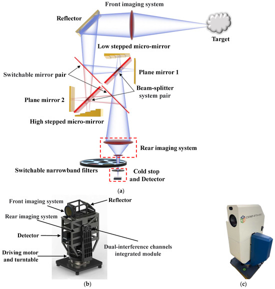
Figure 1.
(a) Simplified internal structure; (b) 3D model of instrument-integrated architecture; (c) real object.
The data acquisition mechanism of the system is as follows: The light emitted by the target object reaches the dual-interference channels integrated module through the front imaging system and the reflector. The module incorporates a broad-band interference channel and a high-resolution interference channel. According to different signal sampling principles, two stepped micro-mirrors with different step heights are used to generate optical path differences (OPDs), and the interference channel is selected by the switchable mirror pair. The chosen light forms two main image points on the plane mirror and the stepped micro-mirror, which are finally imaged on the focal plane of the detector through the rear imaging system and the narrow-band filter.
The height difference between the plane mirror and the stepped micro-mirror causes the OPDs between the two beams of light arriving at the detector to be different, thus forming an interference fringe on the sensor. With rotary stepper scanning by driving the motor and the turntable, the target is imaged onto the next stepped micro-mirror to obtain the interference information of different optical path differences. After completing one scanning cycle, it acquires a three-dimensional data cube containing two-dimensional spatial and one-dimensional spectral information. In the data cube, a series of interference image units with the same interference order are cut and spliced to obtain a two-dimensional scene image of the detection area. The interference image sequence of the same target at all interference orders is extracted for discrete Fourier transform to obtain the target spectrum.
2.2. Dual-Interference Channels Data Sampling Principle
For the broad-band interference channel, according to the classical Nyquist–Shannon sampling theorem, to avoid the aliasing of the reconstructed spectrum, the sampling frequency fs should satisfy the following:
νmax is the maximum wavenumber (corresponding to the minimum wavelength λmin) of the broad-band spectral signal. The sampling step s is 1/fs, the sampling step of the interference system is s ≤ λmin/2, and the λmin in the working band of D-SIFTS is 3.7 μm. Therefore, the sub-step height d1 of the stepped micro-mirror in the broad-band interference channel should satisfy d1 ≤ λmin/4 ≤ 0.925 μm, keeping a certain error margin for the sampling interval and the sub-step height set to 0.625 μm, the spectral resolution ∆ν is as follows:
δmax is the maximum value of the sampling OPDs δ, d is the height of the sub-step, the number of steps N is 160, and the spectral resolution of the broad-band interference channel is 50 cm−1.
For the high-resolution interference channel, the spectral resolution is improved by increasing the maximum sampling OPDs, and the sampling interval will no longer satisfy the classical sampling theorem. According to the bandpass sampling theorem, for it not to occur spectral aliasing phenomenon, the bandpass sampling frequency should be satisfied as follows:
BW is the input signal bandwidth, νL and νH are the minimum and maximum input frequencies, and k is an integer. Equation (3) shows that the sampling frequency fs depends on the signal bandwidth BW and the center wavelength (CWL). The high-resolution interference channel needs to realize the quantitative gas concentration analysis, and its spectral bandwidth should not be too narrow. Therefore, the spectral bandwidth BW is set to 250 cm−1, and fs ≥ 2BW; the sampling step should meet s ≤ 1/(2BW), and the sub-step height d2 should meet d2 ≤ 1/(4BW) ≤ 10 μm. The sub-step height is set to 10 μm to maximize the spectral resolution, and the number of steps N is also 160, so the spectral resolution of this channel is 3.125 cm−1.
This channel requires the bandpass filters to be in front of the detector to limit the bandwidth BW of the incident light signal to a narrow band, as shown in Table 1. The detection band is switched by selecting different bandpass filters on the filter wheel.

Table 1.
High-resolution interference channel bandpass filters.
2.3. Instrument Parameters
The overall parameters of D-SIFTS are shown in Table 2.
Table 2.
Overall parameters of D-SIFTS.
3. Data Processing Algorithm
The data processing process starts from the interferogram data cube obtained by scanning the target scene with D-SIFTS. The specific process is shown in Figure 2.
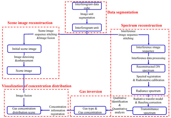
Figure 2.
The flowchart of the data processing algorithm.
The data processing route is divided into two parallel paths: image and spectrum. The image is divided into different interferogram units according to interference orders. In the image processing route, the interferogram units of the same interference order in each image are arranged in the order of the scanning direction to obtain a scene image sequence. Then, image stitching and fusion are carried out to obtain the initial scene image. Finally, image denoising and enhancement are performed to obtain the final scene image. In the spectral processing route, the interferogram units of the same target with different interference orders in each image are stitched according to the OPDs sequence to obtain the interference image sequence of the target. Then, the interference image sequence is resampled, and interferometric intensity baseline correction, apodization, phase correction, and Fourier transform are performed to obtain the digital number (DN) spectrum. It is then subjected to spectral and radiometric calibration to obtain the target radiation spectrum, which is substituted into the radiation transfer equation, and the transmittance baseline correction is performed to obtain the transmittance spectrum. Gas information inversion is performed using the transmittance spectrum of different spectral resolutions and wavenumber intervals obtained via the dual-interference channels to obtain the target material type and concentration information. Finally, the inversion information is registered and fused with the scene image to obtain the gas concentration distribution image.
The interferogram unit is a discontinuous imaging region with different interference intensities formed via interferential modulation of the scene through sub-steps of distinct heights of the stepped mirrors, and its segmentation is the basis for subsequent data processing. The micro-mirror steps determine the interferogram unit’s shape and position. However, due to the micro-mirror fabrication and alignment errors, the interferogram units’ widths of different interference levels are different, and the simple segmentation of the fixed pixel length cannot be used. Instead, it needs to be segmented after edge detection. The edge of the interferogram unit is a straight line of the interference intensity jump caused by the height jump of the sub-step edge of the stepped mirrors. Therefore, this paper chooses the Hough transform curve detection method [34], which has a good effect on the parametric curve detection to segment the interferogram unit, convert the image from two-dimensional coordinate space to parameter space, detect the parameterized 90° straight line, that is, the edge of the unit, and uses the least square fitting to interpolate the detected edge information to obtain the complete edge information, and completes the segmentation and extraction of the interferogram unit.
3.1. Scene Image Reconstruction
3.1.1. Scene Image Stitching
This paper uses a feature-matching-based scene image stitching method. Firstly, the scale-invariant feature transform algorithm (SIFT) is used to extract image features [35,36], and the multiscale Gaussian difference core is constructed. It is convoluted with the image to generate a scale space based on Gaussian difference. In this space, the extreme points are searched as feature points. Finally, the feature matching algorithm based on local maximum entropy matches the feature points to obtain the initial scene image after stitching.
3.1.2. Image Enhancement and Denoising
The bandpass filters in the high-resolution spectral channel cause energy attenuation, which aggravates the inherent problems such as the low contrast and high noise of the infrared images, and there are splicing gaps in the image, reducing image quality. Therefore, this paper proposes a multiscale enhancement algorithm for infrared images incorporating wavelet denoising. The scene image is enhanced in the spatial domain and denoised in the frequency domain to improve image contrast and eliminate the stitching gaps.
Image enhancement based on pyramid transform is a multiscale image enhancement algorithm (MUSICA) that achieves image enhancement by decomposing the image into image pyramids of different sizes and with varying resolutions in the spatial domain and stretching the grey levels of the images in the pyramids directly [37]. The initial scene image is first filtered with a Gaussian kernel and binary down-sampling to construct the image pyramid to obtain a low-resolution approximation. Then, binary up-sampling and inverse filtering are applied to this image to reconstruct an approximation of the current image, and the detailed image of the current scale is obtained by subtracting the approximate image from the current image. The above process is repeated to obtain the low-frequency Gaussian image pyramid of the image and the high-frequency Laplacian image pyramid that represents the details of the image. Let the initial image be G0 (m ≤ Ms, n ≤ Ns) and Ms and Ns be the number of rows and columns of the image, then the lth Gaussian image pyramid Gl is as follows:
i and j denote the position of the image pyramid pixel, L is the layer number of the top layer of the Gaussian image pyramid, Rl and Cl are the numbers of rows and columns of the lth Gaussian image pyramid, and ωg is the Gaussian low-pass filter.
The Laplacian image pyramid is a difference image between an image in the Gaussian image pyramid and its upper level enlarged via interpolation, reflecting the difference in information between the two levels of the Gaussian image pyramid and showing the image details. It is first necessary to interpolate the lth image Gl of the Gaussian image pyramid to obtain the enlarged image G*l so that G*l and Gl−1 have the same size:
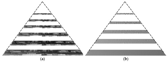
Figure 3.
(a) Gaussian image pyramid; (b) Laplacian image pyramid.
Due to the modulation of the image using the structural features of the stepped micro-mirror, there are many densely arranged stitching gaps in the stitched image. The stitching gaps were analyzed as vertical high-frequency noise and were almost all present in the first layer of the Laplacian image pyramid, as shown in Figure 4b.
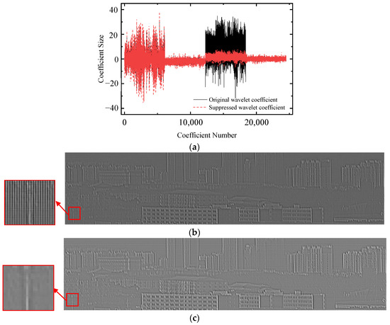
Figure 4.
(a) The first-order wavelet coefficient of the first-layer Laplacian pyramid image; (b) the original first-layer Laplacian pyramid image; (c) the first-layer Laplacian pyramid image after denoising.
Therefore, the image is decomposed using the multiscale first-order wavelet, and the wavelet decomposition coefficients cA, cH, cV, and cD are obtained. The vertical high-frequency wavelet coefficient cV is significantly higher than the horizontal and diagonal high-frequency components. The coefficient is suppressed, and the vertical high-frequency wavelet coefficient cV′ after suppression is as follows:
The positive and negative signs are unchanged before and after suppression, and the vertical high-frequency wavelet coefficient after suppression is similar to the horizontal high-frequency wavelet coefficient, as shown in Figure 4a. Then, it is reconstructed by the multiscale one-dimensional wavelet to obtain a new first-layer Laplacian pyramid image, as shown in Figure 4c.
Combined with the contrast enhancement method of image detail in the traditional MUSICA algorithm, the Laplacian image pyramid of each layer after completing the first layer of wavelet denoising is contrast stretched using exponential transform, and nonlinear enhancement is performed in the spatial domain:
LP′l is the Laplacian pyramid images after the first-layer denoising, LP″l is the Laplacian pyramid images after enhancement, and σ is the exponential coefficient; this paper takes 0.6.
The enhanced high-frequency detail images are up-sampled and interpolated sequentially with the lowest resolution image in the Gaussian image pyramid to achieve high-resolution image pyramid reconstruction.
In addition, to avoid the simultaneous amplification of the detector dark noise in the image enhancement process, in the process of image pyramid reconstruction, each layer of the reconstructed image, in turn, undergoes soft threshold wavelet denoising, as shown in Equation (10), which ultimately leads to the top-level enhanced image of the original scale, as shown in Figure 5.
WT(x) is the high-frequency component of the wavelet coefficient after the first-order wavelet decomposition of the image, T = M∙[ln(Np)/Np]1/2, M is the median of the absolute value of the wavelet coefficient, and Np is the number of pixels in the image.
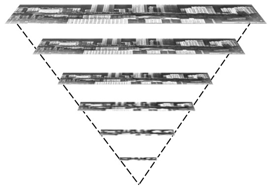
Figure 5.
The high-resolution image pyramid reconstruction: the top layer is the enhanced and denoised original scale image.
3.2. Spectrum Reconstruction
Firstly, according to the OPDs sequence, the interferogram units of different orders of the same target in each image are stitched to obtain the interference image sequence of the target, and the spectrum is obtained by further processing. The main steps are as follows.
3.2.1. Interferometric Intensity Sequence Resampling
Due to unavoidable magnification errors in the imaging system and misalignment of the optics, the interferometric image does not fill the entire detector image plane, resulting in redundant columns of pixels on both sides of the interferogram, as shown in the dotted boxes in Figure 6a,b, which will cause some interferogram units to be modulated by adjacent different interference orders, resulting in light intensity crosstalk and aliasing of interferogram units, further causing uneven distribution of interference fringes and inability to obtain complete interference information, as shown in Figure 6c. Therefore, it is necessary to resample the interferometric intensity sequence to accurately match the target interferometric intensity with its OPDs.
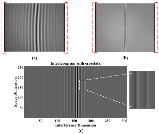
Figure 6.
The interference image sequences of the (a) broad-band interference channel; (b) high-resolution interference channel; (c) interferogram unit crosstalk of high-resolution interference channel.
It is assumed that the interference image sequence after stitching is a ni-column pixel image, and the number of redundant pixel columns on both sides is k1 and k2, respectively. With the accumulation of the width error of the interferogram unit caused by the redundant column pixels, there will be a periodic interferometric intensity order jump:
∆W is the average width error of each interferogram unit, and TJ is the period. Starting from the interferogram unit corresponding to the minimum OPDs, after each TJ sampling with a pixel column interval of 2, the pixel column interval of the following sampling point jumps to 1. After resampling, the interferometric intensity sequence matching the 160-order interference orders is as follows:
Ik represents the kth column pixel in the interference image sequence, and the red term means the sampling interval jump point. The effect of resampling and dimensionality reduction of the interferometric intensity sequence is shown in Figure 7.
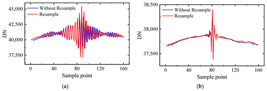
Figure 7.
Interferometric intensity sequence resampling of the (a) broad-band interference channel and (b) high-resolution interference channel.
3.2.2. Interferometric Intensity Baseline Correction
Environmental stray light, circuit instability, and other interfering factors introduced low-frequency noise, and the interferometric intensity sequence, in addition to the cosine modulation of the interference term, were also superimposed on a slowly varying signal component, which is known as the trend term error, and this error leads the baseline of the interferometric intensity sequence to drift, leading to spectral distortion.
Empirical Mode Decomposition (EMD) is a baseline correction method well adapted to stabilize non-stationary signals without any a priori information and signal initial conditions, which is used to decompose the complex spatial light intensity signal I(δ) into a finite number of H intrinsic mode functions (IMF) Ch and trend term r(δ):
Each IMF must satisfy two conditions: (1) the number of extreme points and the number of over-zero points in the spatial domain must be equal or differ by at most 1; (2) at any position, the mean value of the upper envelope formed by the locally maximum points and the lower envelope formed by the locally minimum points must be zero, i.e., the upper and lower envelopes are locally symmetric to the spatial axis. The residual r(δ) is a monotonic function.
The interferometric intensity sequence collected by the high-resolution interference channel (the principle of the broad-band interference channel is the same) is decomposed using EMD to obtain five IMF components and a residual r(δ), as shown in Figure 8. IMF1, IMF2, IMF3, and IMF4 are high-frequency signals. IMF5 and the residual constitute the trend term that causes the baseline drift of the interferometric intensity sequence.
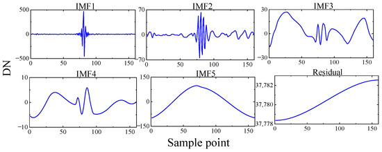
Figure 8.
The interferometric intensity sequence after EMD.
The interferometric intensity baseline correction is performed by removing the baseline composed of the low-frequency trend term IMF5 and the residual. The results are shown in Figure 9.
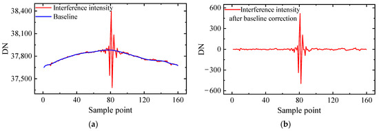
Figure 9.
(a) Baseline of interferometric intensity sequence; (b) interferometric intensity sequence after baseline correction.
3.2.3. Apodization
The sampling cutoff caused by the limited sampling length will lead to sidelobe oscillation of the spectrum, which reduces the spectral SNR. Therefore, it is necessary to smooth the interferometric intensity sequence to suppress the spectral sidelobe oscillation effect, a process known as apodization. It reduces the spectral resolution while suppressing the sidelobe noise to improve the spectral SNR, and the two need to be balanced.
The SNR of the broad-band interference channel is high, and the resolution is low. Therefore, the Happ–Genzel window function with less influence on the spectral resolution is selected:
The high-resolution interference channel has a low spectral SNR due to the filters in its optical path, so the Blackman–Harris window function is used to sacrifice the spectral resolution to maximize the suppression of sidelobe noise:
Δ is the sampling length. The effect of apodization is shown in Figure 10.
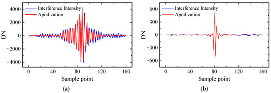
Figure 10.
Apodization of interferometric intensity sequence of (a) broad-band interference channel; (b) high-resolution interference channel.
3.2.4. Phase Correction
Due to fabrication errors in the optical system components, such as those in the stepped micro-mirrors, the delay effect of electronic components related to frequency, the uneven sampling, the interferometric intensity sequence having zero OPDs offset, and asymmetric distortion, introduce a phase error φ(ν), resulting in the distortion of the spectrum and causing photometric errors. The asymmetric interferogram I’(δ) with phase error is expressed as follows:
B(ν) is the ideal spectrum without phase error. The reconstructed spectrum B′(ν) is as follows:
The phase error φ(ν) is
B′r(ν) and B′i(ν) are the real and imaginary parts of the reconstructed spectrum.
The Forman convolution method [38], which has a good correction effect on linear and nonlinear phase errors, is used for phase correction. According to the different effective interference lengths of the dual-interference channels, the small bilateral interferometric intensity sequence of different sizes [39] with high SNR near the zero OPDs is selected to calculate the phase modulation function and convolves with the original interferometric intensity sequence to complete the phase correction (The small bilateral sampling points of the broad-band interferometric intensity sequence and the high-resolution interferometric intensity sequence are 32 and 16 sampling points, respectively). Ic(δ) is the interferometric intensity sequence after phase correction; as shown in Figure 11, the zero OPDs offset error and asymmetric distortion have been significantly improved.
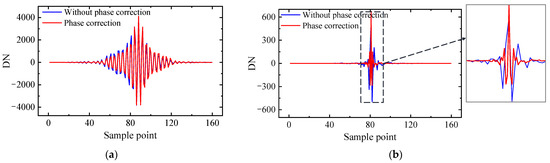
Figure 11.
Phase correction of interferometric intensity sequence in the (a) broad-band interference channel; and (b) high-resolution interference channel.
The Fourier transform of the interferometric intensity sequence Ic(δ) is performed to obtain the original reconstructed DN spectrum Bc(ν):
3.2.5. Spectral and Radiometric Calibration
According to the error transfer model of D-SIFTS [40], the interference core system, composed of plane mirrors, stepped micro-mirrors, beam splitters, and compensation plates, has unavoidable processing and alignment errors. Such errors will lead to linear peak shift and spectral broadening of the reconstructed spectrum:
ν′ is the wave number after shift, ν is the theoretical wave number, and kgain, and boffset are constants. Therefore, the multi-point fitting calibration method is used to perform the first-order linear least squares fitting between the measured spectral wavenumber of each point and its theoretical value for spectral calibration.
After spectral calibration, radiometric calibration can be carried out. That is, the conversion relationship between the spectral responsivity of each spectral channel and the actual radiation flux density of the target is established. Because the D-SIFTS is a linear response system to the external infrared radiation intensity:
K(ν) is the radiation gain coefficient, Lsource(ν) is the target spectral radiance, and Sstray(ν) is the radiation offset caused by the instrument’s thermal radiation. The linear multi-point calibration method is adopted for radiometric calibration. Measuring the reconstructed DN spectra of the blackbody at different temperatures fitted with the theoretical radiation calculated using the Planck function to obtain the radiometric calibration coefficients.
3.2.6. Modeling of Passive Telemetry Radiative Transfer and Baseline Correction of the Transmittance Spectrum
The main application scenario of D-SIFTS is passive telemetry of polluted air masses and gas plumes. Therefore, it is necessary to establish a radiation transmission model, that is, to establish a mathematical model between atmospheric composition information and thermal radiation. Since D-SIFTS mainly uses low elevation angle measurement, a simplified three-layer atmospheric radiative transfer model should be established, as shown in Figure 12.
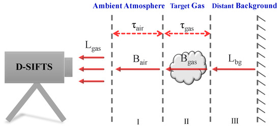
Figure 12.
The radiative transfer model.
According to the model, the total radiance Lgas detected via the D-SIFTS is:
τgas is the transmittance of the target gas, Bgas is the blackbody radiance equal to the temperature of the target gas, Lbg is the radiance of the distant background, τair is the transmittance of the ambient atmosphere, and Bair is the blackbody radiance of the ambient atmosphere temperature. If the transmittance of the ambient atmosphere is equal to 1, simplify Equation (22) to derive the target gas transmittance spectrum:
However, due to the continuous change of instrument state and external environment, the baseline of the gas spectrum drifts. The pseudo-spectral signal will be introduced, affecting the subsequent spectral analysis. Therefore, it is necessary to perform baseline correction.
The baseline correction algorithm used in this paper is the adaptive iterative reweighted penalized least squares method (airPLS), which does not require any prior information and has high correction accuracy. The airPLS algorithm includes the penalized least squares method and adaptive iterative reweighting method, which can balance the fidelity and roughness of the fitted spectrum and add the penalty term to adjust the smoothness of the fitted baseline. The cost function Qt of fitting the spectrum via cyclic iteration is shown in Equation (24). The gas transmittance spectrum τgas(ν) is transformed into the absorbance spectrum A(ν) for baseline correction.
Ai* is the original absorbance spectral vector, Zi* is the fitting spectral vector, the length is ma, t is the number of iterations, θ is the roughness coefficient, and ϕ is the fidelity weight vector (initial value is 0), The iterative formula is as follows:
The termination condition of the loop iteration is to reach the maximum number of iterations or to reach the threshold condition:
dt is the negative difference element between the original spectrum A and the fitting spectrum Zt−1 at the tth iteration. In the above iteration process, the fitting vector of t − 1 times is the undetermined value of the baseline, and the point greater than the unknown value of the baseline is considered a part of the peak. The weight of this point is set to 0, which is ignored in the next iteration fitting. The peak point is gradually eliminated via iteration and reweighting, and the baseline point in the weight vector ϕ is retained to form the fitted spectral baseline. The corrected spectrum is obtained by deducting its fitting baseline, as shown in Figure 13.
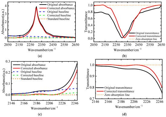
Figure 13.
(a) Broad-band interference channel CO2 absorbance spectrum and baseline; (b) broad-band interference channel CO2 transmittance spectrum after baseline correction; (c) high-resolution interference channel CO2 absorbance spectrum and its baseline; (d) high-resolution interference channel CO2 transmittance spectrum after baseline correction.
3.3. Spectrum Reconstruction
After the gas transmittance spectrum of the dual-interference channels is measured, gas analysis is performed via inversion. The broad-band interference channel has a broad spectral measurement range. In the detection band, the peak position of the measured spectral absorption peak of the gas is compared with the standard spectral absorption peak of the known gas species, and the gas species can be qualitatively identified. The high-resolution interference channel has a high spectral resolution and a narrow spectral detection range, so the spectral detection band can be limited to the characteristic absorption band of a specific gas to analyze the concentration of a single target gas quantitatively.
The partial least squares (PLS) quantitative calibration model is a commonly used quantitative analysis method in spectral analysis, which combines the advantages of principal component analysis, least squares regression, and canonical correlation analysis. The quantitative calibration model is obtained by training the spectral set of known concentration, which is used to predict the concentration information of specific components in the unknown spectrum. Due to the difficulty of obtaining the standard spectrum of a known concentration, the multi-concentration reference spectrum with the same instrument line shape as the D-SIFTS under the known conditions in the HITRAN database is selected as the calibration set to establish the quantitative calibration model. However, there is a nonlinear offset between the absorbance and the gas concentration in the strong absorption region, which will seriously affect the accuracy of the quantitative calibration model, as shown in Figure 14.
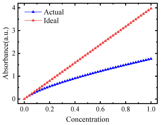
Figure 14.
The nonlinear offset of gas concentration and absorbance.
To eliminate this effect, a segmented partial least squares modeling method is used to divide the spectral calibration set of the wide concentration range of the gas into several calibration sets of the narrow concentration range with good linearity according to the transmittance threshold of the characteristic wavenumber points in the gas detection band. Then, the models were established in several narrow concentration ranges, and the multi-segment regression coefficients were obtained to form the quantitative calibration model of the gas concentration. The specific algorithm flow is shown in Figure 15.
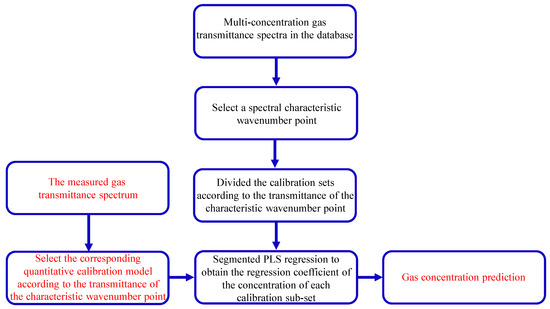
Figure 15.
The gas concentration inversion algorithm.
The gas spectrum of the dual-interference channels of each point in the target area in the passive telemetry scene is inverted to obtain the gas type and concentration information. The accurate matching of the gas concentration information and the spatial position is realized by combining the infrared scene image, the pseudo-color spatial distribution image of the gas concentration is obtained, and the visualization of the gas concentration distribution is realized.
4. Experiments and Results Discussion
Before using the D-SIFTS to carry out experiments to obtain the data, the non-uniformity correction of the HgCdTe detector image surface is first performed to reduce the image noise. As shown in Figure 16, the flatness of the image reaches 99.56%, and the image response can be considered uniform.
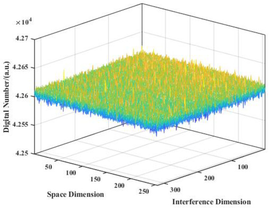
Figure 16.
The image after non-uniformity response correction.
4.1. Panoramic Scanning Imaging
The D-SIFTS is used to perform panoramic scanning imaging of the 30° sector area of the nearby open scene, and the scene is about 2~4 km away from the instrument. In the experiment, the D-SIFTS is located at 43°50′57.52″ north latitude and 125°24′26.82″ east longitude, and the central area of the telemetry scene is located at 43°51′18.07″ north latitude and 125°23′42.54″ east longitude. The interferogram data cube of the scanned scene is shown in Figure 17.
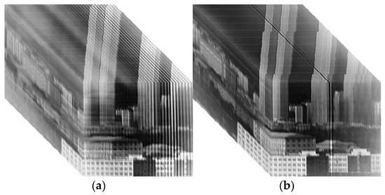
Figure 17.
(a) The interferogram data cube of the broad-band interference channel; (b) the interferogram data cube of the high-resolution interference channel.
Image unit segmentation is performed on the data cube, and the stitching method based on feature matching is used for image stitching to obtain the initial stitching scene image (taking the high-resolution interference channel as an example), as shown in Figure 18a. Then, the multiscale enhancement algorithm for infrared images incorporating wavelet denoising is used to enhance and denoise the initial scene image. Finally, the reconstructed scene image is obtained, as shown in Figure 18b. The original stitching gaps of the image are eliminated, the noise is reduced, the image contrast is enhanced, and the image quality is significantly improved, as shown in Table 3.
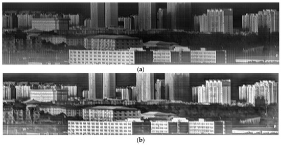
Figure 18.
(a) Initial reconstructed scene image; (b) enhanced and denoised scene image.
Table 3.
Scene image quality before and after image enhancement and denoising.
4.2. Spectral and Radiometric Calibration
Spectral and radiometric calibration experiments need to measure the narrow-band light spectrum formed by different filters in each interference channel when the flat-field radiation source at different temperatures is used as the incident light source. Figure 19 is the spectral calibration and radiometric calibration system built in the laboratory. The flat-field radiation source comprises a face array blackbody and a collimating and beam-expanding system.
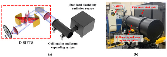
Figure 19.
Spectral and radiometric calibration system (a) schematic diagram; (b) experimental scene.
Firstly, DN spectrum reconstruction is performed on the narrow-band light source corresponding to the dual-interference channels 1st filter when the temperature of the face array blackbody is set to 353 K, as shown in Figure 20a,b. The results show that the reconstructed DN spectrum optimized using the proposed algorithm is consistent with the standard spectrum except for a few linear peak shifts, and the spectral SNR is significantly improved compared to the unoptimized spectrum, which verifies the validity of the DN spectrum reconstruction algorithm.
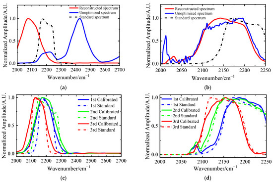
Figure 20.
(a) The 1st filter DN spectrum of the broad-band interference channel. (b) The 1st filter DN spectrum of the high-resolution interference channel. (c) Calibrated reconstructed DN spectrum of narrow-band light sources of the broad-band interference channel. (d) Calibrated reconstructed DN spectrum of narrow-band light sources of the high-resolution interference channel.
Then, by switching the filter wheel, two other filters in Table 1 are selected to form different narrow-band light sources. Then, the error transfer model is obtained by linear fitting the three measured spectra with each wavenumber point in the standard spectra, as shown in Equation (27), and spectral calibration is carried out accordingly. The effect after calibration is shown in Figure 20c,d, and the spectral peak shift and broadening have been well corrected.
The corrected reconstructed DN spectra can be used for radiometric calibration. The temperature range of the face array blackbody is set to 303~353 K (the temperature interval is the typical interval for detecting targets in practical applications of D-SIFTS), and the sampling interval is 10 K, a total of six temperature sampling points. After fitting the radiometric calibration coefficients, the measured DN spectra of the 328 K face array blackbody are used as the verification temperature point for radiometric calibration. The results are shown in Figure 21.
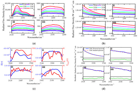
Figure 21.
(a) Reconstructed DN spectrum of each temperature sampling point; (b) theoretical radiance at each temperature sampling point; (c) radiometric calibration coefficients; (d) the radiance and calibration residual after calibration at 328 K temperature point. The serial numbers i, ii, iii, and iiii correspond to the broad-band interference channel and the high-resolution interference channel 1st, 2nd, and 3rd.
The noise equivalent spectral radiance (NESR), which is used to evaluate the noise level of the infrared spectroradiometer, is selected to represent the accuracy of the radiometric calibration experiment results. Furthermore, the concentration detection limit (NECL) of the characteristic gas corresponding to each interference channel is calculated when the temperature difference between the gas and the background is 50 K [41], as shown in Table 4. The NESR of each interference channel is less than 2 × 10⁻⁸ w·(cm2·Sr·cm−1)−1, and the detection limit of the gas concentration meets the actual needs of passive telemetry of gas targets, indicating that the radiometric calibration effect is good.
Table 4.
The NESR and NECL after radiometric calibration of each interference channel.
4.3. Passive Telemetry Simulation of the Gas Target
The gas passive telemetry simulation system was built in the laboratory. The dual-interference channel gas detection experiment was carried out using D-SIFTS, as shown in Figure 22. A face array blackbody infrared radiation light source was used as a background, and the emitted flat-field radiation light passes through the collimator at the entrance pupil of the D-SIFTS. After collimating and expanding the beam, it enters the CaF2 gas pool full of the target gas with a length of 30 cm and a bottom diameter of 10 cm, and finally, it goes through the front imaging system into the D-SIFTS.
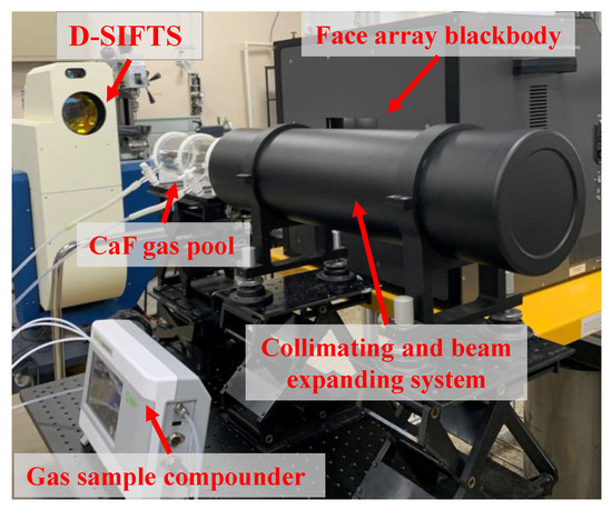
Figure 22.
Experimental scene of the passive telemetry simulation experiment of the gas target.
A spectrum with a gas pool filled with 293 K nitrogen with a face array blackbody temperature set to 353 K is used as the background spectrum. According to the different detection requirements of the dual-interference channels, different types and concentrations of gases with characteristic absorption peaks in the detection band are filled into the gas pool, respectively, as shown in Table 5.
Table 5.
Details of gas detection by dual-interference channels.
The face array blackbody is set to 353 K, and the gas transmittance spectra of each interference channel are obtained. The detection results of the gas transmittance spectra in the broad-band interference channel are shown in Figure 23. The absorption peak positions of various gases are slightly shifted compared with the standard peak positions, as shown in Table 6.
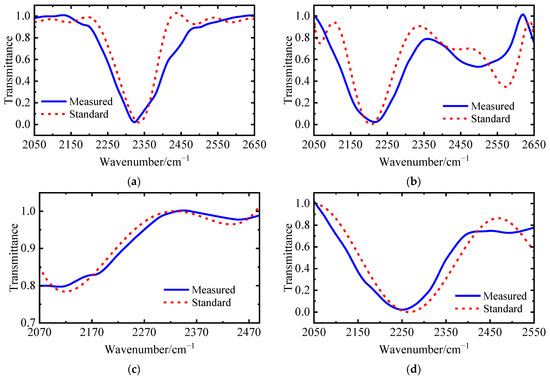
Figure 23.
(a) 10%CO2 transmittance spectrum; (b) 10%N2O transmittance spectrum; (c) 1%CO transmittance spectrum; (d) mixed gas transmittance spectrum.
Table 6.
Peak shift of various gas transmittances in the broad-band channel.
After calculation, the average peak shift of the four gas spectra is 0.4625%, which can meet the needs of a qualitative identification of the detected gas components.
The transmittance detection results of the multi-concentration of each gas in the high-resolution interference channel are shown in Figure 24. The residuals in Figure 24 are the average error between the measured multi-concentration transmittance of each gas and the standard transmittance at the same concentration:
n is the number of gas concentration sampling points, which is six in this experiment. Ti′ is the measured gas transmittance at a specific concentration, and Ti is the standard gas transmittance at this concentration.

Figure 24.
(a) The transmittance of multi-concentration CO2; (b) the transmittance of multi-concentration N2O; (c) the transmittance of multi-concentration CO.
The measured spectra of each gas’s multi-concentration are consistent with the theoretical spectra. The root mean square error (RMSE) of the multi-concentration transmittance spectra and the standard spectra of the three gases were 0.0205,0.0772, and 0.0441, respectively.
Then, according to the gas types, the standard transmittance spectra in the characteristic absorption waveband corresponding to 50 different concentration sampling points of each gas are selected as the total concentration calibration set in the HITRAN database, as shown in Table 7 and Figure 25. The spectral resolution is set to 4 cm−1, and the optical path is 0.3 m.
Table 7.
Spectral parameter information in total gas concentration calibration set.
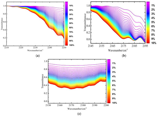
Figure 25.
Concentration calibration set for (a) CO2; (b) N2O; (c) CO.
The total multi-concentration calibration set of each gas is divided into four concentration calibration sub-sets according to the transmittance threshold of the spectral characteristic wavenumber points, and the transmittance and concentration of each spectral point in the sub-sets are modeled using partial least squares regression, and the concentration prediction model of each gas is established. R2 is used as the model accuracy evaluation function, as shown in Equation (29). The closer the value is to 1, the more accurate the model prediction is.
F is the number of samples in the calibration set, cpredicted is the predicted concentration of the model, ctrue is the sample concentration, and ctrue is the average sample concentration. The specific conditions of the segmented concentration quantitative correction model of each gas are shown in Table 8.
Table 8.
Segmented concentration quantitative calibration model of each gas.
The multi-concentration transmittance spectra of the three gases measured using the D-SIFTS high-resolution interference channel are selected to select the corresponding concentration quantitative correction model for concentration prediction. The results are shown in Figure 26.
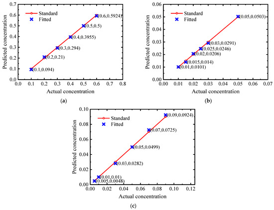
Figure 26.
Predicted concentration of (a) CO2; (b) N2O; (c) CO.
The average relative errors of the concentration inversion of the three gases are 2.38%, 2.53%, and 2.74%, respectively, which verifies the effectiveness of D-SIFTS for high-precision concentration inversion through segmented partial least squares modeling of gas spectra.
4.4. Remote Sensing of Gas Plumes
The D-SIFTS is used to conduct passive telemetry experiments on gas plumes emitted from power plant chimneys. The D-SIFTS is located at 43°50′57.52″ north latitude and 125°24′26.82″ east longitude, and the telemetry target area is located at 43°53′32.37″ north latitude and 125°24′24.65″ east longitude, the telemetry distance is about 4 km, and the chimney has a height of 180 m and a diameter of 5.8 m, as shown in Figure 27.
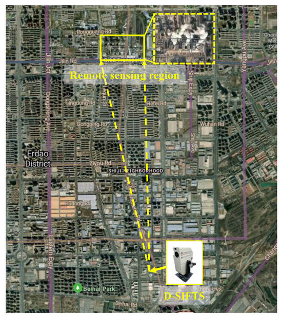
Figure 27.
Experimental scene of remote sensing detection.
By scanning the target area, the three-dimensional interferogram data cubes of the dual-interference channels of the target scene are obtained. Then, the infrared image of the target scene is obtained via scene image reconstruction. A point in the plume emission area is selected for spectral reconstruction to obtain the transmittance spectrum (the gas plume temperature can be obtained in real time from the measured spectrum [42], which is about 68 °C, and the background radiance can be replaced by the measured radiance of the sky point with a similar position, as shown in Figure 28a,b), as shown in Figure 28c,d. Then, the gas transmittance spectrum of the high-resolution interference channel 1st corresponding to each point in a chimney’s gas plume emission area is reconstructed, and the CO2 concentration of each point is inverted by using the quantitative correction model of gas concentration. After registration and fusion of the concentration distribution information and the infrared scene image, the pseudo-color display is performed to realize the spatial visualization of the gas component concentration, as shown in Figure 28e. This area’s maximum CO2 column concentration is about 11.26%∙m, which fits well with the situation [43].
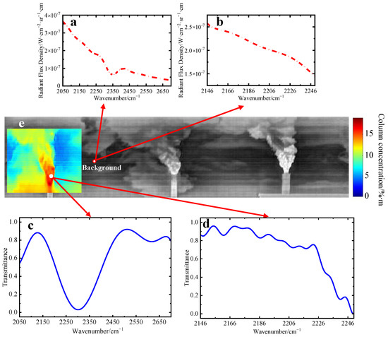
Figure 28.
(a) Background radiance of the broad-band interference channel; (b) background radiance of high-resolution interference channel 1st; (c) transmittance spectrum of the broad-band interference channel; (d) transmittance spectrum of high-resolution interference channel 1st; (e) pseudo-color image of CO2 concentration distribution of gas plume.
5. Conclusions
Based on the D-SIFTS’s unique structural characteristics and data acquisition method, an image and spectrum information processing and gas concentration inversion algorithm suitable for D-SIFTS is proposed. The multiscale enhancement algorithm for infrared images incorporating wavelet denoising eliminates the reconstructed scene image’s stitching gaps, improves the image’s contrast, and reduces the image noise. The image entropy and average gradient increased by 24.07% and 278.74%, respectively. The accuracy of the reconstructed DN spectrum is significantly improved through the use of spectral reconstruction optimization algorithms, such as interferometric intensity sequence resampling and baseline correction, and spectral and radiometric calibration is performed. According to the passive telemetry radiation transmission model, the simulated telemetry experiments of various gases are carried out, the multi-gas transmittance spectra of each interference channel are obtained, and the transmittance baseline correction is carried out. The experimental results show that the average peak drift of the gas transmittance spectrum of the broad-band interference channel is 0.4625%, which meets the needs of qualitative identification. The RMSE between the multi-concentration transmittance spectrum of each gas in the high-resolution interference channel and the theoretical value is 0.0205, 0.0772, and 0.0441. The use of the segmented partial least squares modeling method obtains the quantitative calibration model of gas concentration. Then, the CO2, N2O, and CO gas concentrations are reversed. The average relative error of the concentration inversion of the three gases is less than 3%, which meets the quantitative analysis requirements in terms of gas concentration. Finally, the telemetry experiment is carried out by using D-SIFTS, and the visual display of CO2 concentration distribution in the gas plume of chimney emission is preliminarily realized, which verifies the excellent application value and potential of D-SIFTS in environmental emergency monitoring and daily emission detection in industrial parks.
Author Contributions
Conceptualization, G.L. and J.L. (Jinguang Lv); methodology, G.L. and J.L. (Jinguang Lv); validation, G.L., J.L. (Jinguang Lv), B.Z. and Y.C.; investigation, G.L., Y.Z. and K.S.; resources, B.Z.; writing—original draft preparation, G.L.; writing—review and editing, J.L. (Jingqiu Liang) and W.W.; supervision, Y.Q. and K.Z.; funding acquisition, J.L. (Jingqiu Liang) and S.W. All authors have read and agreed to the published version of the manuscript.
Funding
This research was funded by the Jilin Scientific and Technological Development Program under Grant 20230201049GX, Grant 20230508141RC and Grant 20230508137RC; funded by the National Natural Science Foundation of China under Grant 61805239, Grant 61627819 and 61727818; funded by the Youth Innovation Promotion Association Foundation of the Chinese Academy of Sciences under Grant 2018254; and funded by the National Key R&D Program of China under Grant 2022YFB3604702.
Data Availability Statement
The data presented in this study are available upon request from the corresponding author. The data are not publicly available due to the data need to be used for further research.
Conflicts of Interest
The authors declare no conflicts of interest. The funders had no role in the design of the study; in the collection, analyses, or interpretation of data; in the writing of the manuscript, or in the decision to publish the results.
References
- Griffiths, P.R. Fourier transform infrared spectrometry. Science 1983, 222, 297–302. [Google Scholar] [CrossRef] [PubMed]
- Yang, C.; Zhou, Z.-Y.; Li, Y.; Liu, S.-K.; Ge, Z.; Guo, G.-C.; Shi, B.-S. Angular-spectrum-dependent interference. Light Sci. Appl. 2021, 10, 217. [Google Scholar] [CrossRef] [PubMed]
- Israelsen, N.M.; Petersen, C.R.; Barh, A.; Jain, D.; Jensen, M.; Hannesschläger, G.; Tidemand-Lichtenberg, P.; Pedersen, C.; Podoleanu, A.; Bang, O. Real-time high-resolution mid-infrared optical coherence tomography. Light Sci. Appl. 2019, 8, 11. [Google Scholar] [CrossRef] [PubMed]
- Saptari, V. Fourier Transform Spectroscopy Instrumentation Engineering; SPIE Optical Engineering Press: Bellingham, WA, USA, 2003. [Google Scholar]
- Talghader, J.J.; Gawarikar, A.S.; Shea, R.P. Spectral selectivity in infrared thermal detection. Light Sci. Appl. 2012, 1, e24. [Google Scholar] [CrossRef]
- Li, A.; Yao, C.; Xia, J.; Wang, H.; Cheng, Q.; Penty, R.; Fainman, Y.; Pan, S. Advances in cost-effective integrated spectrometers. Light Sci. Appl. 2022, 11, 174. [Google Scholar] [CrossRef] [PubMed]
- Zhang, C.; Zhao, B.; Xiangli, B.; Li, Y. Interference image spectroscopy for upper atmospheric wind field measurement. Optik 2006, 117, 265–270. [Google Scholar] [CrossRef]
- Girshovitz, P.; Shaked, N.T. Doubling the field of view in off-axis low-coherence interferometric imaging. Light Sci. Appl. 2014, 3, e151. [Google Scholar] [CrossRef]
- Pope, A.; Rees, W.G. Impact of spatial, spectral, and radiometric properties of multispectral imagers on glacier surface classification. Remote Sens. Environ. 2014, 141, 1–13. [Google Scholar] [CrossRef]
- Shang, S.; Lee, Z.; Lin, G.; Hu, C.; Shi, L.; Zhang, Y.; Li, X.; Wu, J.; Yan, J. Sensing an intense phytoplankton bloom in the western Taiwan Strait from radiometric measurements on a UAV. Remote Sens. Environ. 2017, 198, 85–94. [Google Scholar] [CrossRef]
- Kaiser, F.; Vergyris, P.; Aktas, D.; Babin, C.; Labonté, L.; Tanzilli, S. Quantum enhancement of accuracy and precision in optical interferometry. Light Sci. Appl. 2018, 7, 17163. [Google Scholar] [CrossRef]
- Zhang, C.; Liu, C.; Chan, K.L.; Hu, Q.; Liu, H.; Li, B.; Xing, C.; Tan, W.; Zhou, H.; Si, F. First observation of tropospheric nitrogen dioxide from the Environmental Trace Gases Monitoring Instrument onboard the GaoFen-5 satellite. Light Sci. Appl. 2020, 9, 66. [Google Scholar] [CrossRef] [PubMed]
- Garoi, F.; Nicolae, I.; Prepelita, P. Monochromatic light measurement via geometric phase and Fourier-transform spectroscopy method. Sci. Rep. 2022, 12, 12922. [Google Scholar] [CrossRef] [PubMed]
- Hase, F.; Frey, M.; Blumenstock, T.; Groß, J.; Kiel, M.; Kohlhepp, R.; Mengistu Tsidu, G.; Schäfer, K.; Sha, M.; Orphal, J. Application of portable FTIR spectrometers for detecting greenhouse gas emissions of the major city Berlin. Atmos. Meas. Tech. 2015, 8, 3059–3068. [Google Scholar] [CrossRef]
- Wiacek, A.; Hellmich, M.; Flesch, T. Application of Open-Path Fourier Transform Infrared (OP-FTIR) Spectroscopy to Air-Sea Greenhouse Gas Exchange. In Fourier Transform Spectroscopy; Optica Publishing Group: Washington, DC, USA, 2021; p. JW4D.1. [Google Scholar]
- Soncco, D.-C.; Barbanson, C.; Nikolova, M.; Almansa, A.; Ferrec, Y. Fast and accurate multiplicative decomposition for fringe removal in interferometric images. IEEE Trans. Comput. Imaging 2017, 3, 187–201. [Google Scholar] [CrossRef]
- Kattnig, A. Theoretical and practical analysis of spatial and spectral calibration of static Fourier transform infrared spectrometers. Opt. Express 2019, 27, 14819–14834. [Google Scholar] [CrossRef] [PubMed]
- Xu, Y.; Li, J.; Bai, C.; Wei, M.; Liu, J.; Wang, Y.; Ji, Y. Iterative local Fourier transform-based high-accuracy wavelength calibration for Fourier transform imaging spectrometer. Opt. Express 2020, 28, 5768–5786. [Google Scholar] [CrossRef] [PubMed]
- Hu, Y.; Xu, L.; Shen, X.; Jin, L.; Xu, H.; Deng, Y.; Liu, J.; Liu, W. Reconstruction of a leaking gas cloud from a passive FTIR scanning remote-sensing imaging system. Appl. Opt. 2021, 60, 9396–9403. [Google Scholar] [CrossRef] [PubMed]
- Chen, T.; Su, X.; Li, H.; Li, S.; Liu, J.; Zhang, G.; Feng, X.; Wang, S.; Liu, X.; Wang, Y. Learning a Fully Connected U-Net for Spectrum Reconstruction of Fourier Transform Imaging Spectrometers. Remote Sens. 2022, 14, 900. [Google Scholar] [CrossRef]
- Cho, J.Y.; Lee, S.; Kim, H.; Jang, W.K. Spectral Reconstruction for High Spectral Resolution in a Static Modulated Fourier-transform Spectrometer. Curr. Opt. Photonics 2022, 6, 244–251. [Google Scholar]
- Shu, Y.; Sun, J.; Lyu, J.; Fan, Y.; Zhou, N.; Ye, R.; Zheng, G.; Chen, Q.; Zuo, C. Adaptive optical quantitative phase imaging based on annular illumination Fourier ptychographic microscopy. PhotoniX 2022, 3, 24. [Google Scholar] [CrossRef]
- Ding, X.; Wang, Z.; Hu, G.; Liu, J.; Zhang, K.; Li, H.; Ratni, B.; Burokur, S.N.; Wu, Q.; Tan, J.; et al. Metasurface holographic image projection based on mathematical properties of Fourier transform. PhotoniX 2020, 1, 16. [Google Scholar] [CrossRef]
- Kleinert, A.; Friedl-Vallon, F.; Guggenmoser, T.; Höpfner, M.; Neubert, T.; Ribalda, R.; Sha, M.; Ungermann, J.; Blank, J.; Ebersoldt, A. Level 0 to 1 processing of the imaging Fourier transform spectrometer GLORIA: Generation of radiometrically and spectrally calibrated spectra. Atmos. Meas. Tech. 2014, 7, 4167–4184. [Google Scholar] [CrossRef][Green Version]
- Coudrain, C.; Bernhardt, S.; Caes, M.; Domel, R.; Ferrec, Y.; Gouyon, R.; Henry, D.; Jacquart, M.; Kattnig, A.; Perrault, P. SIELETERS, an airborne infrared dual-band spectro-imaging system for measurement of scene spectral signatures. Opt. Express 2015, 23, 16164–16176. [Google Scholar] [CrossRef] [PubMed]
- Zhang, C.; Li, Q.; Yan, T.; Mu, T.; Wei, Y. High throughput static channeled interference imaging spectropolarimeter based on a Savart polariscope. Opt. Express 2016, 24, 23314–23332. [Google Scholar] [CrossRef] [PubMed]
- Yan, T.; Zhang, C.; Zhang, J.; Quan, N.; Tong, C. High resolution channeled imaging spectropolarimetry based on liquid crystal variable retarder. Opt. Express 2018, 26, 10382–10391. [Google Scholar] [CrossRef] [PubMed]
- Li, Q.; Lu, F.; Wang, X.; Zhu, C. Low crosstalk polarization-difference channeled imaging spectropolarimeter using double-Wollaston prism. Opt. Express 2019, 27, 11734–11747. [Google Scholar] [CrossRef] [PubMed]
- Gao, L.; Cao, L.; Zhong, Y.; Jia, Z. Field-Based High-Quality Emissivity Spectra Measurement Using a Fourier Transform Thermal Infrared Hyperspectral Imager. Remote Sens. 2021, 13, 4453. [Google Scholar] [CrossRef]
- ElZeiny, W.E.; Sabry, Y.M.; Khalil, D.A. Complex Kernel-based spectrum reconstruction algorithm for cascaded Fabry–Perot interferometric spectrometer. Appl. Opt. 2021, 60, 8999–9006. [Google Scholar] [CrossRef]
- Hu, Y.; Xu, L.; Xu, H.; Shen, X.; Deng, Y.; Xu, H.; Liu, J.; Liu, W. Three-dimensional reconstruction of a leaking gas cloud based on two scanning FTIR remote-sensing imaging systems. Opt. Express 2022, 30, 25581–25596. [Google Scholar] [CrossRef]
- Shi, H.; Xiong, W.; Ye, H.; Wu, S.; Zhu, F.; Li, Z.; Luo, H.; Li, C.; Wang, X. High Resolution Fourier Transform Spectrometer for Ground-Based Verification of Greenhouse Gases Satellites. Remote Sens. 2023, 15, 1671. [Google Scholar] [CrossRef]
- Ren, J.; Lü, J.; Zhao, B.; Wang, Q.; Qin, Y.; Tao, J.; Liang, J.; Wang, W. Optical design and investigation of a dual-interference channels and bispectrum static fourier-transform imaging spectrometer based on stepped micro-mirror. IEEE Access 2021, 9, 81871–81881. [Google Scholar] [CrossRef]
- Ballard, D.H. Generalizing the Hough transform to detect arbitrary shapes. Pattern Recognit. 1981, 13, 111–122. [Google Scholar] [CrossRef]
- Lowe, D.G. Distinctive image features from scale-invariant keypoints. Int. J. Comput. Vis. 2004, 60, 91–110. [Google Scholar] [CrossRef]
- Gong, M.; Zhao, S.; Jiao, L.; Tian, D.; Wang, S. A novel coarse-to-fine scheme for automatic image registration based on SIFT and mutual information. IEEE Trans. Geosci. Remote Sens. 2013, 52, 4328–4338. [Google Scholar] [CrossRef]
- Vuylsteke, P.; Schoeters, E.P. Multiscale image contrast amplification (MUSICA). In Medical Imaging 1994: Image Processing; SPIE: Bellingham, WA, USA, 1994; pp. 551–560. [Google Scholar]
- Lichun, M.; Renzhong, Y.; Lu, S. Improvement and implementation of Forman phase correction algorithm. Remote Sens. Nat. Resour. 2013, 25, 97–101. [Google Scholar]
- Xiang, Y.; Yuan, Y. Research on data processing methods of unilateral interferograms. Acta Photonica Sin. 2006, 35, 12. [Google Scholar]
- Zhao, B.; Liang, J.; Lv, J.; Zheng, K.; Zhao, Y.; Chen, Y.; Sheng, K.; Qin, Y.; Wang, W. Reducing the Influence of Systematic Errors in Interference Core of Stepped Micro-Mirror Imaging Fourier Transform Spectrometer: A Novel Calibration Method. Remote Sens. 2023, 15, 985. [Google Scholar] [CrossRef]
- Jiao, Y.; Xu, L.; Gao, M.; Jin, L.; Tong, J.; Li, S.; Wei, X. Investigation of the Limit of Detection of an Infrared passive Remote Sensing and Scanning Imaging System for Pollution Gas. Spectrosc. Spectr. Anal. 2013, 33, 2617–2620. [Google Scholar]
- Jiao, Y.; Xu, L.; Gao, M.; Jin, L.; Tong, J.; Li, S.; Wei, X. Real-time data processing of remote measurement of air pollution by infrared passive scanning imaging system. Acta Phys. Sin. 2013, 62, 140705. [Google Scholar] [CrossRef]
- Gao, M.; Liu, W.; Zhang, T.; Liu, C.; Liu, J.; Wei, Q.; Lu, Y.; Wang, Y.; Zhu, J.; Xu, L. Passive FTIR Remote Sensing of Gaseous Pollutant in Heated Plume. Spectrosc. Spectr. Anal. 2006, 26, 47–50. [Google Scholar]
Disclaimer/Publisher’s Note: The statements, opinions and data contained in all publications are solely those of the individual author(s) and contributor(s) and not of MDPI and/or the editor(s). MDPI and/or the editor(s) disclaim responsibility for any injury to people or property resulting from any ideas, methods, instructions or products referred to in the content. |
© 2024 by the authors. Licensee MDPI, Basel, Switzerland. This article is an open access article distributed under the terms and conditions of the Creative Commons Attribution (CC BY) license (https://creativecommons.org/licenses/by/4.0/).