Abstract
Unsupervised person re-identification (Re-ID) aims to match the query image of a person with images in the gallery without the use of supervision labels. Most existing methods usually generate pseudo-labels through clustering algorithms for contrastive learning, which inevitably results in noisy labels assigned to samples. In addition, methods that only apply contrastive learning at the clustering level fail to fully consider instance-level relationships between instances. Motivated by this, we propose a joint contrastive learning (JCL) framework for unsupervised person Re-ID. Our proposed method involves creating two memory banks to store features of cluster centroids and instances and applies cluster and instance-level contrastive learning, respectively, to jointly optimize the neural networks. The cluster-level contrastive loss is used to promote feature compactness within the same cluster and reinforce identity similarity. The instance-level contrastive loss is used to distinguish easily confused samples. In addition, we use a WaveBlock attention module (WAM), which can continuously wave feature map blocks and introduce attention mechanisms to produce more robust feature representations of a person without considerable information loss. Furthermore, we enhance the quality of our clustering by leveraging camera label information to eliminate clusters containing single camera captures. Extensive experimental results on two widely used person Re-ID datasets verify the effectiveness of our JCL method. Meanwhile, we also used two remote sensing datasets to demonstrate the generalizability of our method.
1. Introduction
Person Re-ID aims to recognize the same person across various camera views. In recent years, researchers have devoted themselves to designing new network structures and efficient loss functions for supervised person Re-ID, aiming to learn cross-camera recognition feature representations and achieve satisfactory results. Nevertheless, supervised person Re-ID [1,2,3,4,5] are data-driven and require substantial human and time costs to annotate the data, which limits the expandability of supervised methods. Therefore, increasing research is directed towards unsupervised person Re-ID to extract discriminative features directly from unlabeled data, which has greater deployment potential in real-world scenarios.
Prior studies regarding unsupervised person Re-ID have investigated many effective solutions [6,7,8,9,10], which fall into two main categories. One of the primary categories involves the utilization of the unsupervised domain adaptation (UDA) [11,12,13,14,15] approach, which revolves around creating a unified model that bridges the source and target domain and achieving domain migration through feature alignment and domain adaptation on the target domain. The second category is a purely unsupervised (PU) [16,17,18,19,20,21] method that directly uses unannotated data to update the model. PU presents greater challenges since it does not require a labeled source domain dataset.
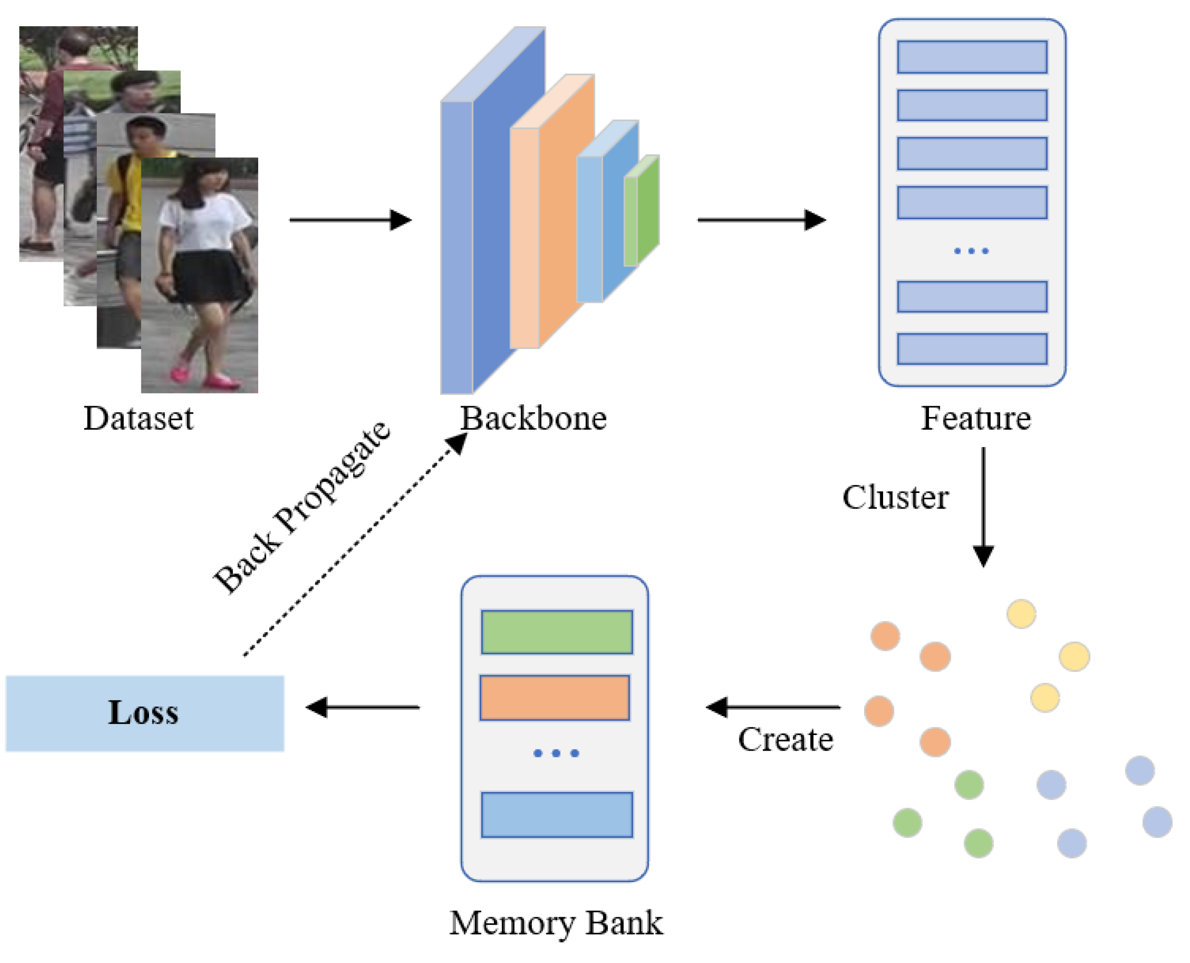
Existing PU methods typically predict pseudo-labels and memory banks for unlabeled training samples by utilizing clustering algorithms as supervised information for model updates, as shown in Figure 1. The first part is to feed unannotated images into the network to extract corresponding feature embeddings, which are then saved in the memory bank. The second step applies a clustering algorithm to cluster the image features, after which each cluster is assigned a pseudo-label. The third step involves feature representation learning achieved through contrastive learning. The fundamental distinction of these approaches lies in the design of various memory banks to achieve different effects. For example, to make full use of all samples, MMCL [11] treated each image as a single instance and updated the memory bank to calculate the instance-level loss. The memory bank of SPCL [6] stored cluster centroid and outlier features and used contrastive learning to distinguish source-domain classes and target-domain clusters. To enhance the compactness of instance features belonging to the same identity, CCL [17] constructed a memory at the cluster level to store central features, thereby mitigating the issue of intra-class update inconsistency.
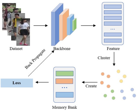
Figure 1.
Illustration of existing PU methods. Such methods utilize clustering algorithms to obtain pseudo-labels and calculate the averaged momentum representations of each cluster to initialize the cluster-level memory bank.
Although clustering-based PU methods have demonstrated impressive performance, there are still some challenges that need to be tackled. First of all, because of the cross-camera character of the Re-ID task, a person may be captured by multiple cameras [22]; hence, the resulting clusters comprise samples from distinct camera sources. When using unlabeled datasets, clustering often produces noisy labels, which will cause the model to update in the wrong direction and severely damage the model’s performance. Secondly, applying cluster-level contrastive learning does not take into account the structural relationship among instances and does not fully utilize their feature information. Finally, the training instances that hold the highest value and provide the most information come from different cameras or different perspectives of the same person. However, due to the complexity of the shooting environment, different pedestrians usually look similar in the same camera view.
To address the aforementioned issues, we propose a joint contrastive learning (JCL) method. Firstly, we use a WaveBlock attention module (WAM) to extract more discriminative features and then propose a cluster-filtering approach in the clustering stage to optimize the results. Secondly, we design a cluster-level and an instance-level memory bank and then jointly train the model by using contrastive loss based on the memory bank, respectively. For instance-level contrastive loss, we propose an instance screening strategy to select instances with medium similarity for improving the reliability of positive samples.
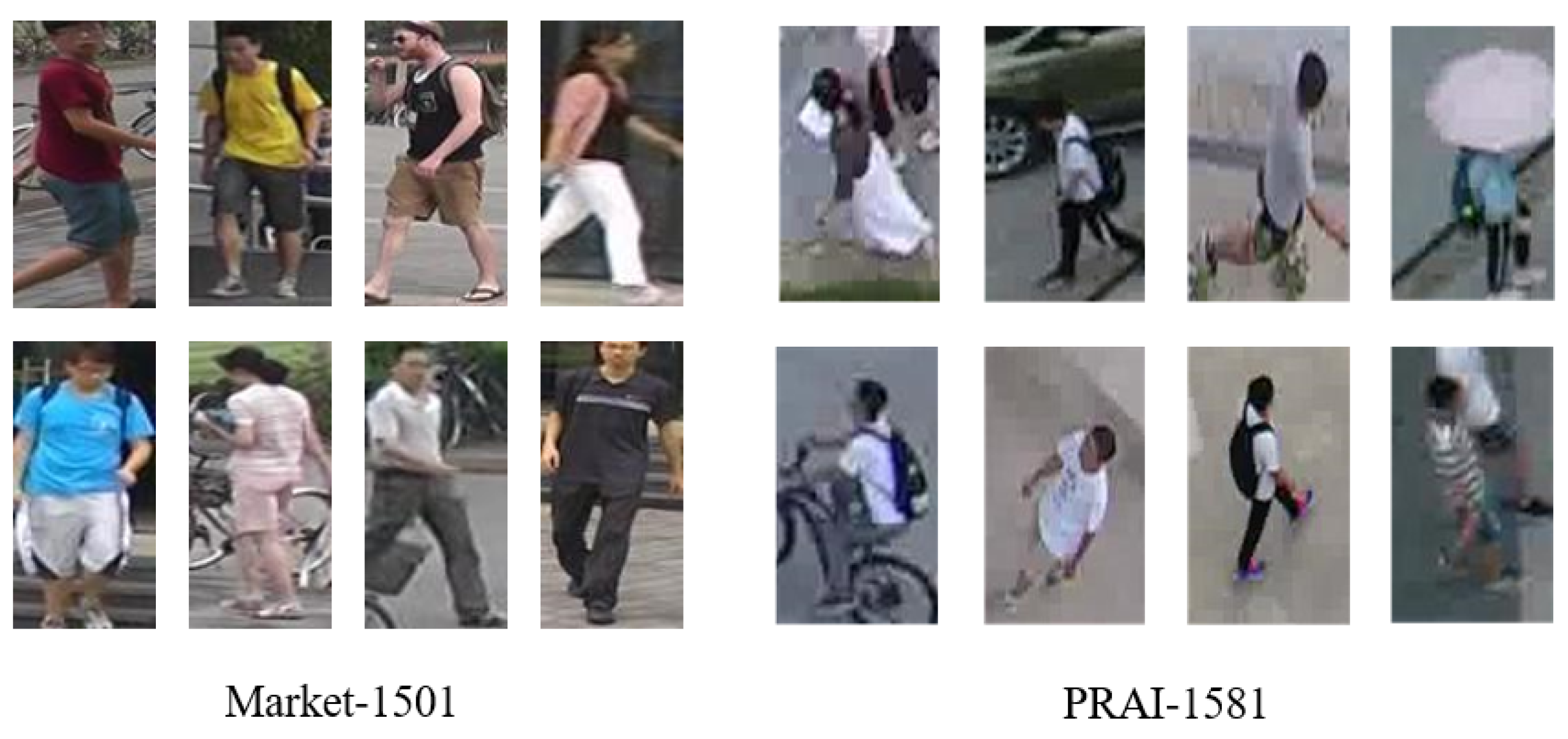
Meanwhile, in the current era marked by the swift progress of unmanned aerial vehicles (UAVs) nowadays, the integration of UAV platforms for video surveillance has emerged as an essential complementary strategy for conventional stationary camera systems. With the emergence of person Re-ID datasets PRAI-1581 [23] captured by UAVs, research in aerial images has become possible. Compared to the images captured by other stationary cameras, the images captured by UAVs from the top show that each person has a very different posture, similar appearance, low resolution, and occlusion, making them more challenging. To showcase the broad applicability and efficacy of our proposed model, we also conducted experiments on PRAI-1581 to assess its performance. In addition, we perform visualization experiments on a challenging remote sensing dataset, Xiongan New Area [24], to further showcase the generalization capability of our approach. The dataset consists of numerous intricate objects, encompassing diverse categories such as rice, elm, poplar, and more, predominantly featuring farmlands.
In conclusion, our proposed method has several contributions, which are as follows:
- We propose a joint contrastive learning (JCL) framework that combines cluster-level and instance-level contrastive losses to jointly optimize models. By applying the instance screening strategy, the reliability of positive samples can be effectively improved, which is beneficial for model training.
- We design a cluster-filtering approach to eliminate clusters containing single camera captures by leveraging camera label information. To obtain more discriminative features of a person, we adopt a WaveBlock attention module (WAM) to directly apply the attention mechanism to different fluctuation regions.
- Extensive experimental results with impressive performance verify the efficacy of our proposed approach.
2. Related Works
2.1. Unsupervised Person Re-ID
Previous research on unsupervised person Re-ID can be categorized into two main groups: unsupervised domain adaptive (UDA) and purely unsupervised (PU).
The UDA method’s goal is to achieve domain migration through feature alignment and domain adaptation on the target domain. As there exist substantial differences between domains, various methods reduce the distinctions by performing feature distribution alignment and image style conversion. For instance, SPGAN [25] utilized CycleGAN [26] for the transformation of images and employed a source domain label during model training. However, these approaches are not entirely effective due to the inability to effectively explore the correlation between instances in the target domain during the migration process. MMT [12] proposed enhancing the robustness of pseudo labels through the process of mutual learning.
PU method presents greater challenges compared to the UDA method since it exclusively employs unlabeled data for model training. As a result, establishing robust feature representations becomes more challenging in the absence of labeled training samples. In unsupervised learning, researchers commonly employ optimal clustering and memory banks so that positive and negative samples can be directly obtained from the memory bank in their work. For example, Lin et al. [18] devised a clustering process that operates from the bottom up and incorporated a diversity regularization term to equilibrate data volume within each cluster. MMCL [11] utilized a memory-based non-parametric classifier and transformed the target task into a multilabel classification problem. CCL [17] constructed a memory at the center level to store cluster representations and updated them during the training process to avoid propagating noise instances to the next training process, which helps improve the distinguishing ability of features during the training process.
2.2. Attention Mechanism
The attention mechanism was originally introduced in the visual image field to improve the traditional visual search method [27,28], which tries to discover discriminative or key features to promote the representation capability of the model so as to address the task of mining person information in person Re-ID. Therefore, lots of researchers attempted to apply attention mechanisms to person Re-ID. The relationship perception attention (RGA) module [1] is designed to explicitly explore the global active domain relations and the excavation of structural information, which helps to infer semantics, thereby increasing attention. HLGAT [29] injected attention regularization loss to limit the weight of local features and combine context information to consider structural information. In our research, we leverage the attention mechanism to identify the crucial or negative features that impact accuracy.
2.3. Contrastive Learning
Contrastive learning aims to extract distinctive features from datasets by enabling the model to discern similarities and differences among the data. It can be regarded as the process of looking up the dictionary [30], that is, selecting a person with the same identity in the candidate set mixed with many negative samples. When dealing with a substantial quantity of negative samples, contrastive learning can work better because more negative samples can effectively cover the underlying data distribution. Drawing inspiration from this, certain recent works have made efforts to employ contrastive learning in tackling the challenge of unsupervised person Re-ID. CAP [8] uses camera labels to divide each cluster into varying numbers of proxies and includes the intra- and inter-camera contrastive losses. CACL [31] is an asymmetric contrastive learning framework aimed at enabling networks to effectively utilize more effective information beyond color. Compared to previous methods, our JCL is built at the instance and cluster granularity. It focuses on guiding the learning process with positive instances with high confidence and hard negative instances.
2.4. Visual Tasks on Remote Sensing Images
In recent academic endeavors, there has been a growing focus on remote-sensing images, and the majority of research efforts have centered around tasks such as object detection and classification. Hong et al. [32] introduced an innovative backbone network designed to acquire local spectral sequence information from neighboring bands of remote sensing images. Meanwhile, there are also some of the most advanced unsupervised learning technologies in the area of remote sensing. Tao et al. [33] introduced a unified feature learning framework to learn image features by using limited labeled or unlabeled data. Huang et al. [34] introduced a clustering algorithm tailored for hyperspectral images, which enhances the model’s resilience to noise through the incorporation of an adaptive spatial regularization technique. [35] merges the spatial and spectral features within the Siamese tracker. However, there is limited attention paid to person Re-ID tasks using remote sensing images. With the proposal of the UAV person Re-ID dataset PRAI-1581 and the widespread attention of intelligent air surveillance systems, person Re-ID based on remote sensing images has received attention from researchers. In the dataset PRAI-1581, all images are taken at an altitude of 20–60 m from the ground, making UAV person Re-ID more challenging. The variable flight altitude and adjustable camera angle allow people to have different resolutions, perspectives, and postures in a drone. Additionally, due to the independent control of two drones in the PRAI-1581, the entire scene is more complex, greatly meeting the research needs of person Re-ID in remote sensing images.
3. Method
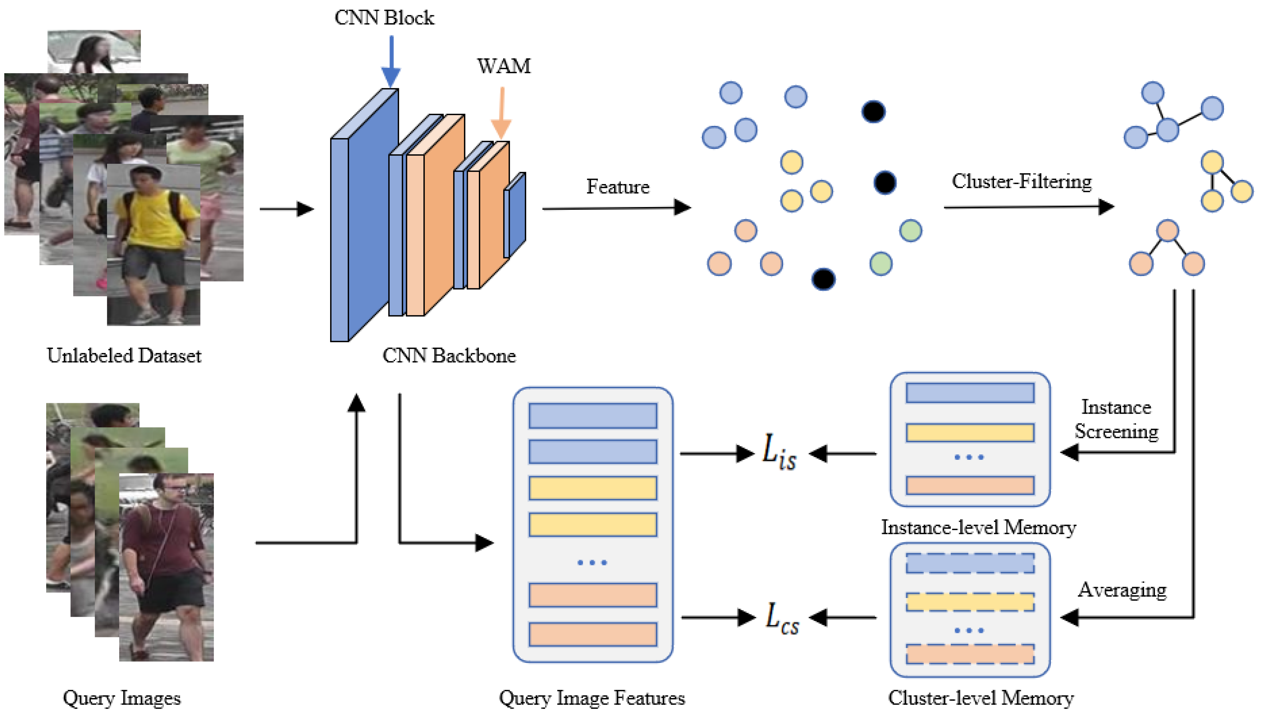
We propose a joint contrastive learning (JCL) framework, which consists of three primary modules: a feature extraction module, a cluster optimization module, and a joint contrastive learning module. The overall framework is depicted in Figure 2.
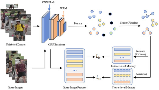
Figure 2.
Illustration of JCL. Our method alternates between the feature extraction stage, clustering stage, and training stage. In the feature extraction stage, we employ ResNet-50 combined with WAM to capture image features from unlabeled datasets. Subsequently, we divide the extracted features into various clusters as pseudo labels and enhance cluster reliability through the clustering optimization module. Finally, a joint contrastive learning method according to cluster-level and instance-level memory banks serves to enhance the feature recognition capability of the model.
3.1. Approach Overview
Denote as the training set without labels, encompassing N images. The encoder is responsible for extracting image features, represented as . Let represent the features extracted from model and .
In the clustering stage, we employ the DBSCAN method to cluster the extracted image features, after which a cluster filtering strategy is used to eliminate outlier instances and clusters containing only single camera captures to filter out reliable clusters. We subsequently allocate identical pseudo labels to instances that are part of the same cluster. Finally, we can obtain a novel labeled dataset, denoted as , where means the cluster labels, is the number of instances, and Q represents the count of clusters. We calculate the average value of all instance features from a cluster as the cluster centroid represented as .
By utilizing memory banks to store image features, we use the cluster-level contrastive loss (CLL) and instance-level contrastive loss (ILL) for training. The complete loss function is as follows:
where represents CLL, represents ILL, and parameter is a balancing factor between 0 and 1, which mainly affects the weight of CLL and ILL.
3.2. Feature Extraction Module
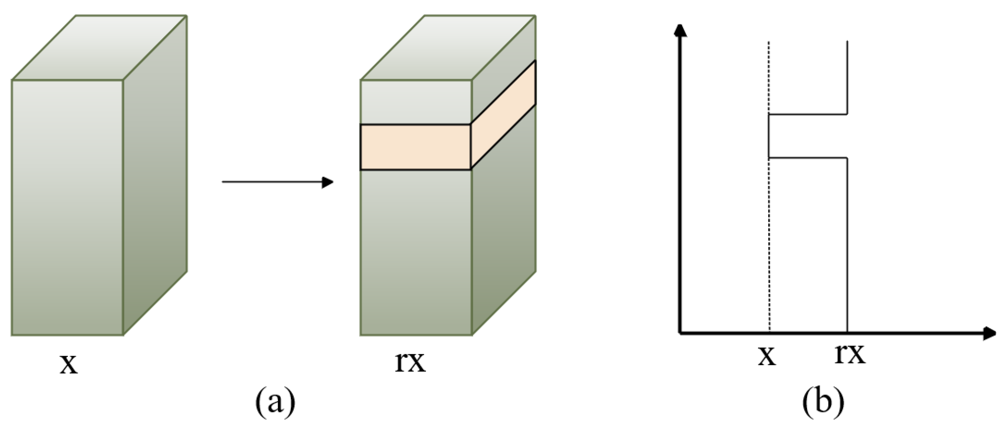
To investigate the features of various body modules of a person, we introduced the WaveBlock [36] module as an alternative to dropping blocks, which may have the potential to cause the loss of discriminative features. Figure 3 illustrates the pipeline of WaveBlock. It uses various bands to adjust the feature map, produces the feature map with increased discriminative information, and partially retains the original information.

Figure 3.
Overview of the WaveBlock module, where x represents the value of extracting the person-image feature blocks and r is the wave rate. A block is chosen randomly and remains unchanged, while feature values of the remaining blocks are multiplied by r times. (a) represents the selected feature block, while (b) describes the way in which the feature values are changed.
We position the attention mechanism following the WaveBlock, called the WaveBlock attention module (WAM), and the attention mechanism we use is a non-local block, which includes two branches. Consider as the feature map of a non-local block, and let represent a convolution. In the first branch, through , the feature map F undergoes a reduction in the number of channels to half of the previous one, denoted as . In a similar fashion, another convolution, denoted as , reduces the channel count to half of its original value, denoted as . We compress the spatial dimensions of and into a single dimension, denoted as , . We obtain the matrix as follows:
In another branch, the feature map F is input into a convolution g followed by a batch normalization layer denoted as . We compress the spatial dimension of and then use a transpose to obtain . Then, we perform multiplication between J and , followed by a transpose and reshaping of its dimensions to . Finally, we employ an additional convolution h to revert the channel dimension back to C. We use E to represent the output result and then add E and F for the final feature representation.
3.3. Cluster Optimization Module
Due to differences in lighting [37] and views between cameras, the features of distinct persons captured by the same camera are prone to clustering together within a cluster, leading to the generation of inaccurate pseudo labels. Meanwhile, as person Re-ID is a cross-camera task, where each person is captured by multiple cameras, the camera labels for the same person image in the dataset should not be entirely the same.
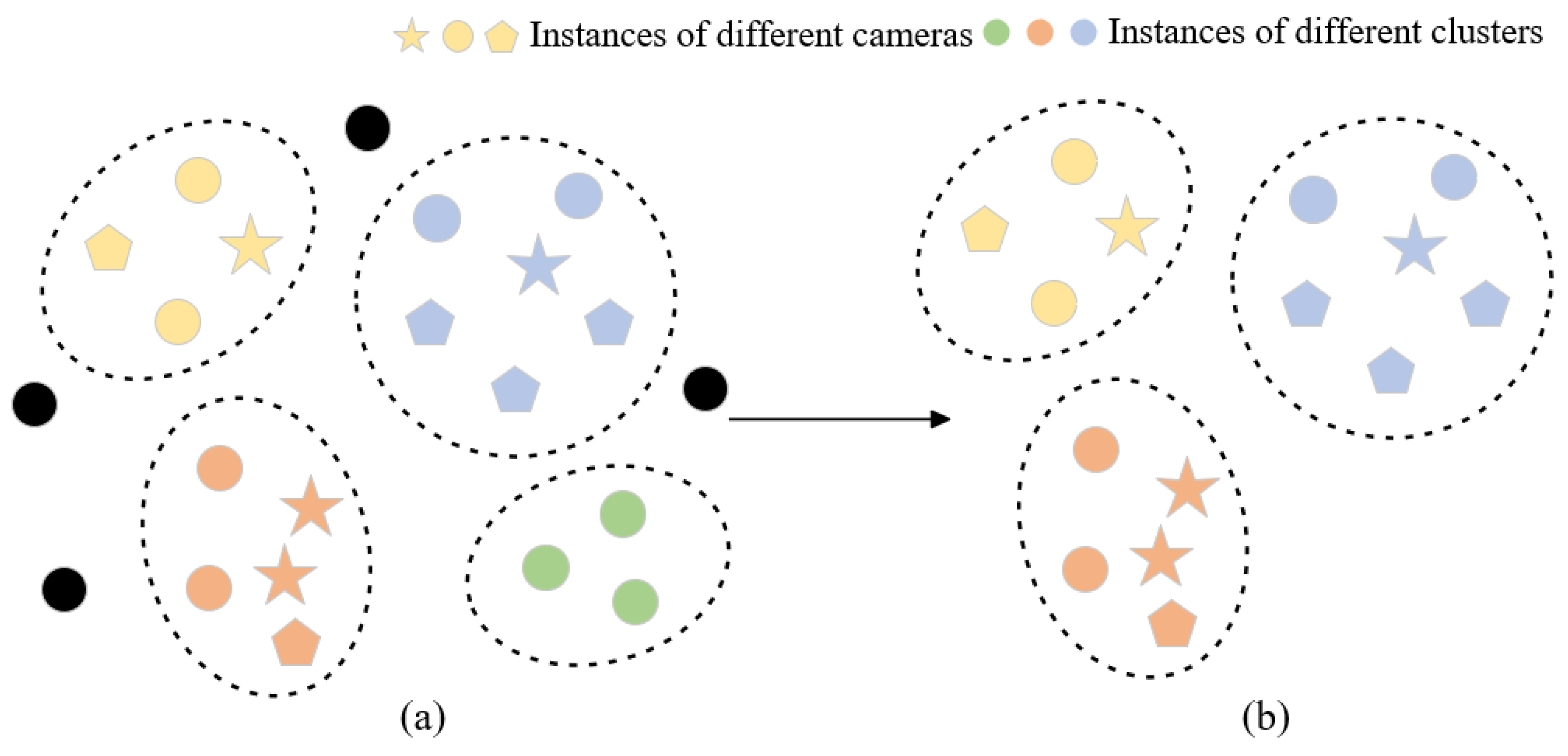
In order to filter out more reliable clusters, we developed a cluster-filtering approach that leverages camera-based data and evaluates the number of cameras within a cluster to remove outlier instances and clusters captured by a single camera, thereby optimizing reliability. We only keep clusters containing samples captured by multiple cameras and then select trustworthy clusters to continue model training while minimizing the impact of extraneous noise labels. Figure 4 illustrates the clustering optimization process and outlier instances (black dots), and single-camera clusters (green dots) have been removed through the clustering optimization module.
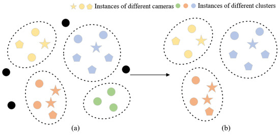
Figure 4.
Visual representation of the feature space (a) prior to and (b) subsequent to the cluster optimization module. Distinct shapes indicate various cameras, while varying colors represent belonging to different clusters. Black means outlier instances.
3.4. Joint Contrastive Learning Module
We propose a joint contrastive learning (JCL) that combines CLL and ILL.
In CLL, we use the cluster-level memory bank to reserve unique cluster representation features for each cluster. Regardless of the size of the cluster, we update the corresponding features in to ensure the consistency of clusters and then use ClusterNCE loss [17] to calculate CLL, as follows:
where q is a query instance feature, denotes the unique representation vector of cluster i, represents the centroid feature of the cluster to which the query instance q belongs, and denotes the temperature hyperparameter.
We compute the centroid of clusters and then save them in . We employ the average value of all instance features from a cluster as the initial value for the cluster representation, as follows:
where represents the sample set in the i-th cluster, represents the number of instances. Only after one epoch is completed, the cluster centroid is updated once through consistency, and the update process is as follows:
where m represents a momentum updating factor for updating cluster features. undergoes updates by q following each training iteration.
To further explore the relationship among instances, we designed an instance-level contrastive loss (ILL) and proposed an instance screening strategy. Firstly, we establish an instance-level memory bank for preserving the filtered instance features within each cluster, which contains G instances in Q clusters. Specifically, we find the cluster to which q belongs through distance measurement. By calculating the similarity rank between q and all instances in the cluster, we filter out middle-ranked instances to obtain a more reliable positive sample. For other clusters, the instances closest to q are selected as the negative samples for contrastive learning, as illustrated in Figure 5. Our instance screening strategy takes into account the comprehensive relationships between each query instance and clusters featuring diverse pseudo-labels. We generate a set of Q sample pairs, comprising one positive sample pair and hard negative pairs, and our ILL is defined as follows:
where represents the instance temperature hyperparameter, is the instance feature with the middle-ranked cosine similarity within the same pseudo label, and denotes the hard negative instance feature, which corresponds to the i-th cluster and exhibits the highest-ranked cosine similarity. and are defined as:
and

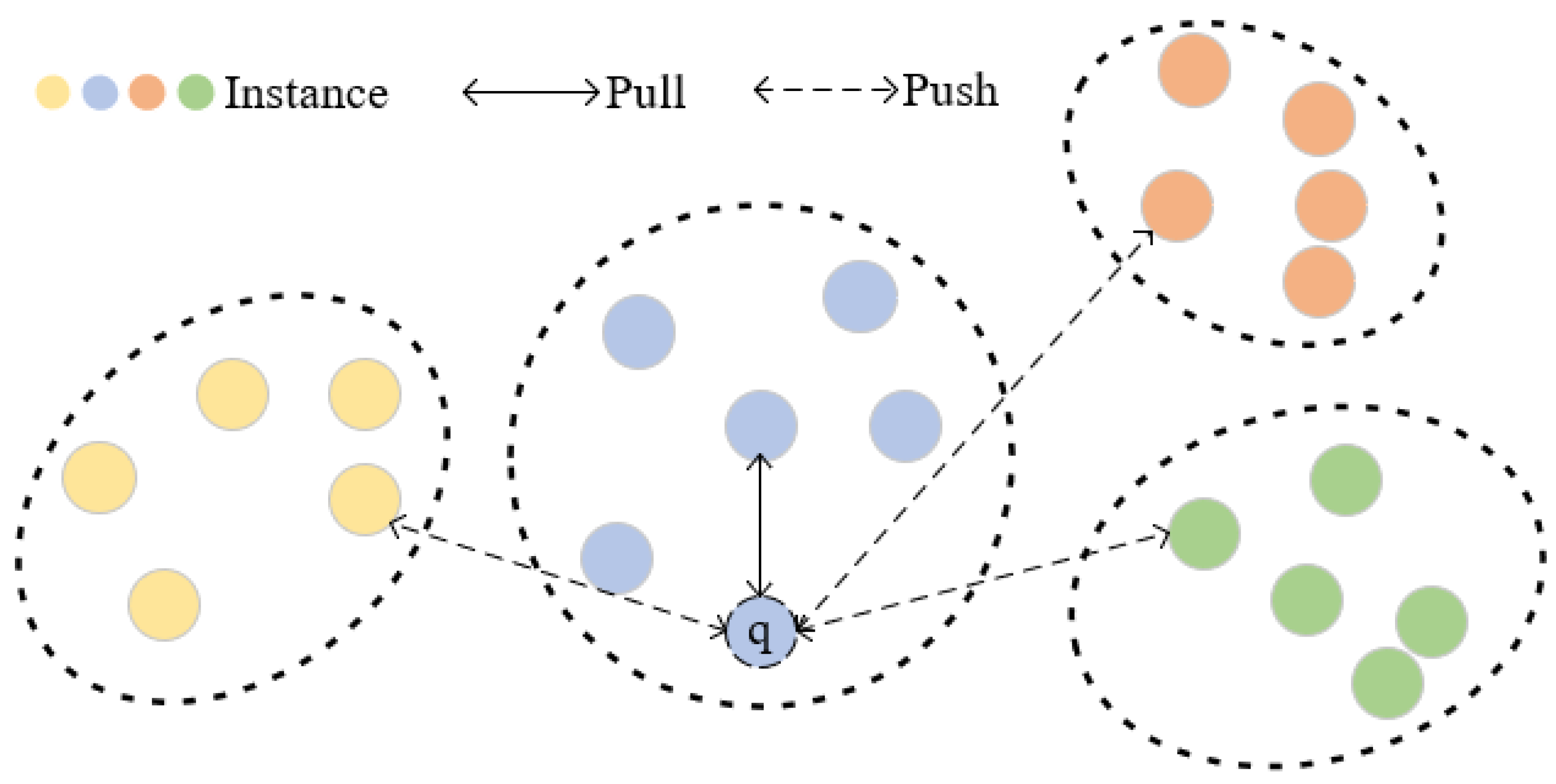
Figure 5.
Visual representation of feature space for ILL. Each point represents the features of the image, and different colors are used to represent various identities, where q is a query instance. The ILL we formulated effectively improves the similarity between the query instance and positive sample by minimizing the distance between them while pushing away negative samples.
Similarly, in each training iteration, we refresh all instance features corresponding to a mini-batch and revise the memory bank as follows:
We outline the entire procedure of our approach in Algorithm 1.
| Algorithm 1 Unsupervised Person Re-ID with Joint Contrastive Learning |
|
4. Experiments
4.1. Datasets and Evaluation Metrics
To demonstrate the efficacy of our suggested approach, we assessed the proposed technique on two extensive benchmark person Re-ID datasets and two remote sensing datasets, namely Market-1501 [38], DukeMTMC-reID [39], PRAI-1581 [23] and Xiongan New Area [24].
Market-1501 [38]: this dataset comprises 12,936 images belonging to 751 unique identities within the training set, while the testing set includes 19,732 images split into a query set consisting of 3368 images and a gallery set consisting of 16,364 images. The dataset comprises six distinct non-overlapping cameras, and each individual identity in the dataset has been recorded by a minimum of two separate cameras.
DukeMTMC-reID [39]: this dataset comprises 16,522 images in the training set, which are distributed among 702 identities. The testing set of the dataset is composed of 19,889 images with the remaining 702 identities. It comprises eight different cameras, ensuring that each identity in the dataset has been recorded by at least two different cameras.
PRAI-1581 [23]: this dataset comprises 39,461 images featuring 1581 person identities. The training set comprises 19,523 images representing 781 identities, while the testing set of the dataset is composed of 19,938 images with the remaining 799 identities. Within the testing set, 4680 images associated with 799 distinct identities are designated as query images. These images are captured from two separate drones, operating at altitudes varying between 20 m and 60 m above ground level. The proportion of incorrect labels in this dataset is approximately 5%.
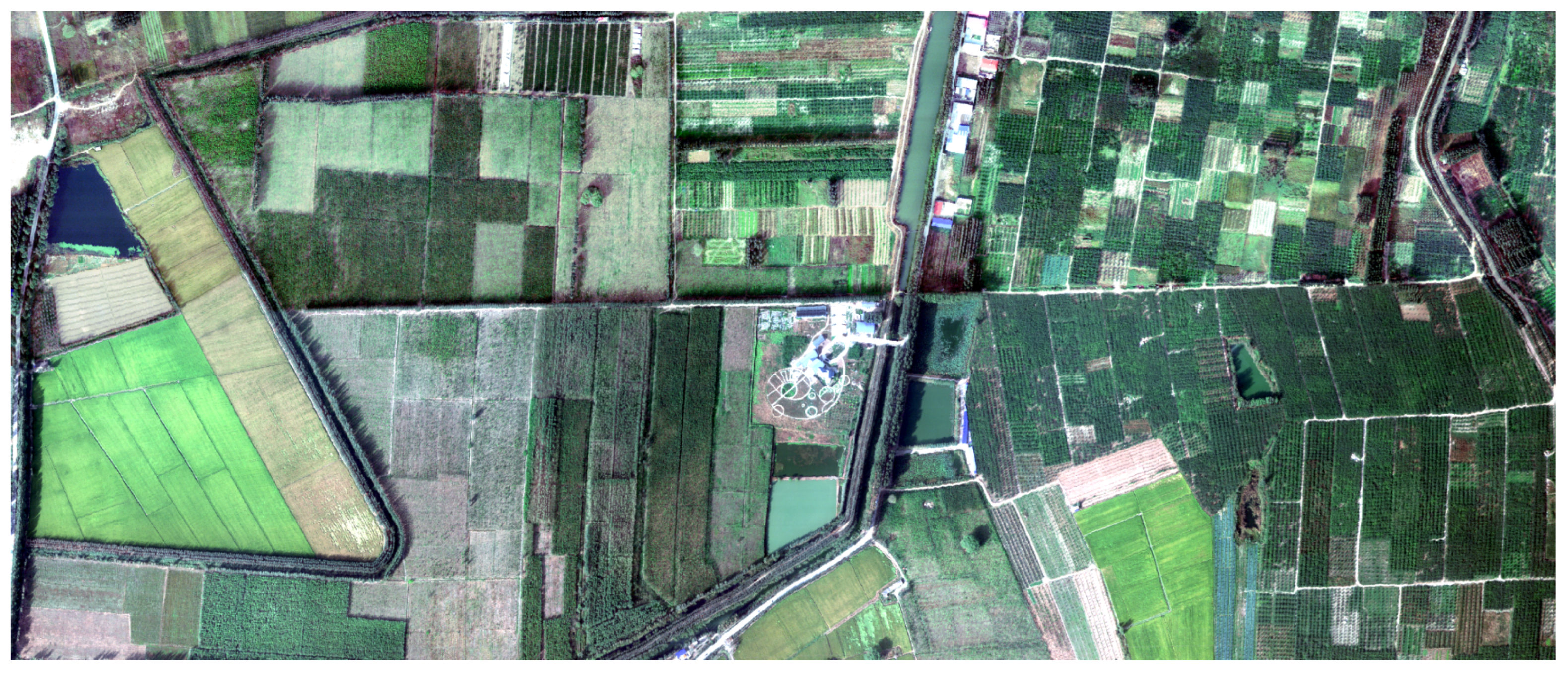
Xiongan New Area [24]: the Xiongan dataset constitutes a hyperspectral image (HSI) captured in Matiwan Village within the Xiongan New Area of China. The dataset is acquired using a spectrometer specifically designed for visible and near-infrared imaging. It covers a spectral range of 400∼1000 nm with 256 bands, and the spatial resolution is configured at 0.5 m, resulting in an image size of pixels. This dataset comprises various finely detailed entities, primarily consisting of cultivated lands, as shown in Figure 6. The Xiongan New Area dataset includes 19 types of objects, such as rice, grassland, elm, willow, etc. The specific objects and sample sizes are shown in Table 1.
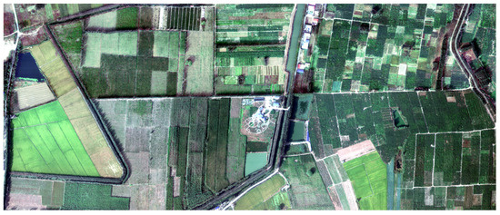
Figure 6.
The examples are sourced from the Xiongan New Area dataset, which includes 19 land cover types, and among them, agricultural and forestry vegetation are the main research objects.

Table 1.
Number of object samples in the Xiongan New Area dataset.
Evaluation metrics: training does not include ground truth identities. We assessed the effectiveness of the JCL method using established training/test segmentation and evaluation protocols. We adopted two standard metrics, namely cumulative matching characteristic (CMC) [40] and mean average precision (mAP).
4.2. Implementation Details
ResNet-50 [41], pre-trained by ImageNet [42], is adopted as the backbone encoder for the feature extraction, and all input images are resized to 256 × 128. Upon layer 4, we removed all layers and introduced global average pooling (GAP), a batch normalization layer [43], and an L2-normalization layer, resulting in the generation of 2048 dimensional features. When conducting testing, we utilize the features extracted from GAP to compute the distance. We calculate the Jaccard distance [3] and employ DBSCAN [44] algorithms to generate pseudo labels, and the thresholds are set as 0.55 on Market-1501 [38] or 0.6 on DukeMTMC-reID [39]. Regarding training images, we perform random horizontal flipping, random erasing, and random cropping. Each mini-batch comprises 256 images representing 16 pseudo identities, with each person having 16 instance samples. We utilize an Adam optimizer to facilitate the training of the model, employing a weight decay of 5 . The initial learning rate is established at 3.5 and then decreases to of its prior value every 20 epochs spanning 60 epochs.
4.3. Comparison with Existing Methods
We conducted a comparative analysis between our method and several of the newest unsupervised methods, which roughly fall into two categories: (1) UDA methods, (2) PU methods. Table 2 presents the performance metrics of these approaches on two distinct datasets. Our method achieves % in mAP and % in rank-1 accuracy on DukeMTMC-reID and % in mAP and % in rank-1 accuracy on Market-1501.

Table 2.
Comparison with the state-of-the-art unsupervised Re-ID methods on Market-1501 and DukeMTMC-reID, employing ResNet-50 as the backbone model. Bold indicates the best performance.
Comparison with UDA methods. Due to the ability to leverage information from labeled source domain datasets, UDA methods (e.g., SPCL [6], MMCL [11], and MET [14]) usually exhibit better performance than PU methods. The results displayed in Table 2 highlight the exceptional efficacy of our proposed approach even without any identity annotations, surpassing the UDA method utilizing labeled source domain data. As an illustration, our approach achieves % improvement for Rank-1, a % increase for mAP on Market-1501, and delivers % Rank-1 and % mAP enhancement on DukeMTMC-reID compared to second-ranked approach RESL.
Comparison with PU methods. We evaluated the efficacy of our approach by comparing it to several PU methods. As shown in Table 2, our proposed method significantly outperforms all compared PU methods (e.g., CCL [17], CAP [8], P2LR [13], CACL [31], O2CAP [9]). As an illustration, our method achieves a minimum of % and % increase in Rank-1 and % and % improvement in mAP on Market-1501 and DukeMTMC-reID, respectively.
4.4. Ablation Study
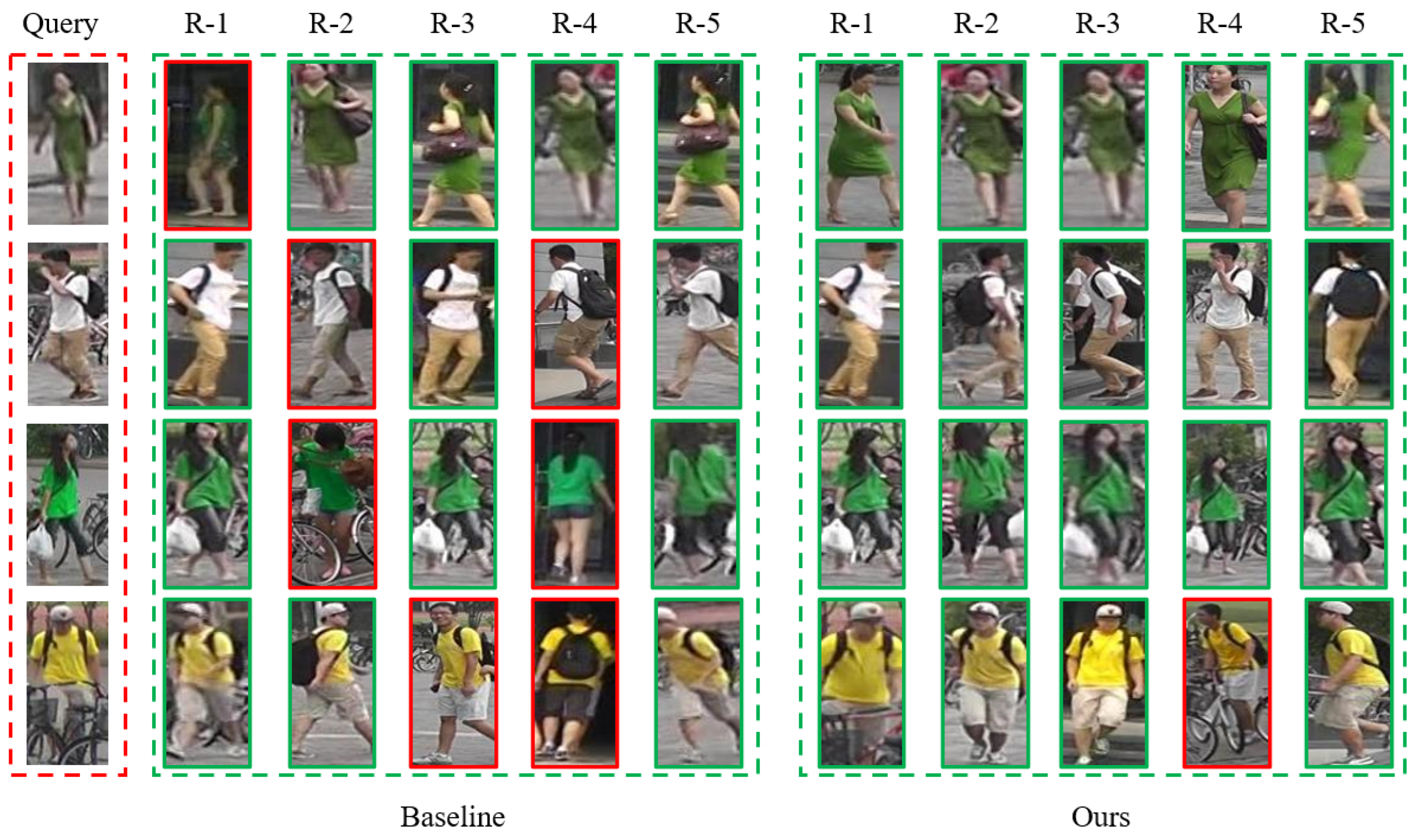
We aim to showcase the efficacy of various modules within our proposed approach by conducting a series of ablation experiments on two datasets. We adopted the SPCL [6] model as our baseline, and the results of the ablation experiments are presented in Table 3. It is evident that our complete model outperforms the baseline on all datasets. We present visual representations of the retrieval outcomes achieved by both the baseline and JCL methods. As shown in Figure 7, the gallery instances retrieved are indicated by green bounding boxes if they match the query instances. On the contrary, the ones denoted with red bounding boxes represent individuals with identities distinct from the query instances. It is evident that our approach can differentiate between visually similar images, a capability not exhibited by the baseline.

Table 3.
Ablation studies on different modules. ILL denotes instance-level contrastive loss; CLL denotes cluster-level contrastive loss; JCL denotes joint contrastive loss; WAM denotes the WaveBlock attention module; COM denotes the cluster optimization module. Bold indicates the best performance.
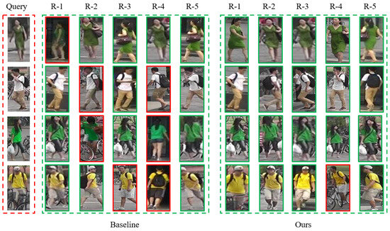
Figure 7.
Comparing the top-5 ranking lists between baseline and our method on Market-1501. Images with green borders indicate correct matches, while those with red borders signify incorrect matches.
Effectiveness of joint contrastive learning module. Our proposed JCL module aims to comprehensively consider cluster-level and instance-level information through joint contrastive learning. When we compare the outcomes of (d) and (a) in Table 3, it becomes evident that the efficacy of the JCL module is clear. From variant (b) and variant (c), when we only use ILL or CLL, the performance is still better than the baseline on all datasets.
Effectiveness of the WaveBlock attention module. Our model employs WAM to obtain more discriminative features in images to enhance the accuracy of clustering results. Upon reviewing the comparative outcomes between variant (e) and variant (d) in Table 3, it becomes evident that our introduced WAM module has a beneficial impact on the model’s performance across all datasets. This confirms the essential role of the WAM module. We achieve a % increase in Rank-1 and % improvement in mAP on Market-1501. Additionally, there is a % improvement in Rank-1 and % increase in mAP on DukeMTMC-reID.
Effectiveness of the cluster optimization module. In order to prove the superiority of the cluster optimization module (COM), we compare the efficacy of the model after adding COM. The results are shown in rows (e) and (f) of Table 3, we obtain % mAP gain on Market-1501 and % mAP gain on DukeMTMC-reID, which indicates that the COM is effective for screening reliable instances.
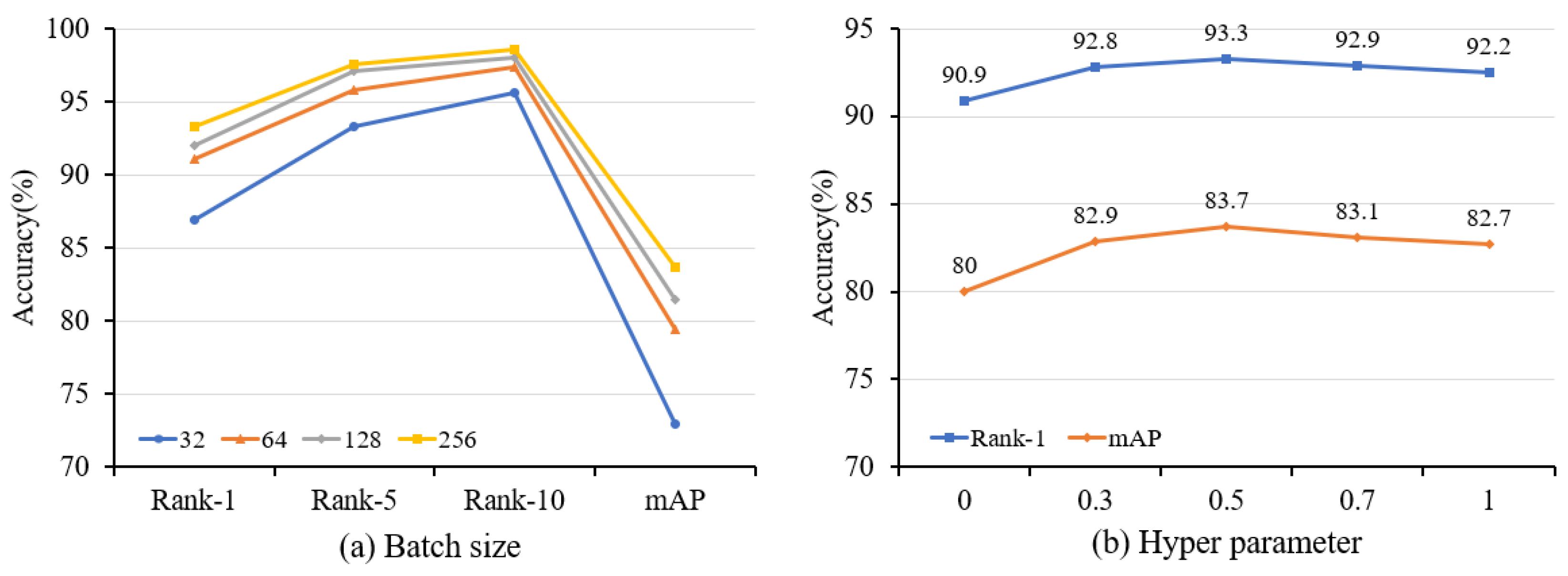
The influence of batch size. To investigate the influence of varying batch sizes, we conducted training experiments using batch sizes that ranged from 32 to 256. Based on the experimental findings presented in Figure 8a, our proposed method achieves the highest accuracy for two datasets when a batch size of 256 is selected.
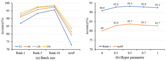
Figure 8.
Ablation study with different settings of (a) batch size and (b) hyperparameter on Market-1501. The batch size refers to the amount of data selected by the model for processing during the training process, while the hyperparameter is used to control the impact of the loss function.
The influence of hyperparameter. The hyperparameter serves as a balancing factor, ranging from 0 to 1, and its main role is to affect the weight between CLL and ILL. Figure 8b shows the experimental results under various . When is 0, the model is only trained by ILL, which hampers the acquisition of generalized features. Meanwhile, the noise pseudo labels, for instance, have a great impact on the model. On the contrary, when is 1, only CLL is used. While it is possible to diminish the impact of noise, retaining only a single feature for each cluster leads to a loss of intra-class feature diversity. We obtain the best performance when the two losses are combined, and is set as 0.5.
The influence of the clustering threshold. As shown in Table 4, the clustering threshold significantly influences the number of pseudo-labels generated and thus has a profound influence on the overall performance of our methods. Setting the threshold too high results in multiple samples being grouped into the same cluster, leading to an abundance of erroneous pseudo-labels. Conversely, if the threshold is established exceedingly low, samples attributed to the equivalent person ID will fragment into numerous diminutive clusters, which does not contribute favorably to model enhancement. To identify the most suitable threshold value, we conduct ablation experiments on two datasets, as illustrated in Table 5 and Table 6. The highest performance is attained on the Market-1501 dataset with a threshold of 0.55, while on DukeMTMC-reID, the optimal outcome is attained when setting a threshold of 0.6. The difference in clustering thresholds is due to the large size of the DukeMTMC-reID dataset, the large number of cameras, and the more complex background environment, making it more difficult to recognize person images than in Market-1501. This will result in a lower similarity between the same person image features, so setting a larger threshold will increase the constraint distance between instances in the clustering process, and more instances will be merged into one cluster to achieve better performance.

Table 4.
The quantity of pseudo-labels produced at under various clustering thresholds on Market-1501, where the number of pseudo labels represents the number of clusters after clustering.

Table 5.
The influence of various clustering thresholds on Market-1501. Showing the values of rank-r and map (%). The best results are in bold.

Table 6.
The influence of various clustering thresholds on DukeMTMC-reID. Showing the values of rank-r and map (%). The best results are in bold.
The influence of IBN-ResNet and Generalized Mean Pooling. Furthermore, we also investigate the influence of several commonly employed tricks on our method, such as IBN-ResNet and generalized mean (GeM) [42] Pooling. As illustrated in Table 7, our proposed JCL’s performance can be enhanced further by incorporating IBN-ResNet and GeM [42] on two datasets.

Table 7.
The impact of different tricks on our proposed method JCL on two real-world person Re-ID datasets. ’IBN’ indicates the use of IBN-ResNet50. ‘GeM’ indicates the generalized mean pooling layer. The best results are in bold.
4.5. Experiments in Remote Sensing Dataset
To highlight the flexibility of our methodology, we perform experiments on the extensive airborne person Re-ID dataset PRAI-1581 [23], encompassing 39,461 images portraying 1581 person identities. The dataset comprises images captured by two UAVs during flight, encompassing a wide range of real UAV surveillance scenarios.
As a result of the UAV’s varying flight altitudes, the camera’s adjustable tilt angle, and the fuselage’s ability to freely rotate, people exhibit a wide range of resolutions, perspectives, and poses within the dataset. The complexity of the overall situation is further elevated. Figure 9 shows some example images in the PRAI-1581, and the remote sensing person images are more challenging than those captured by traditional fixed cameras.
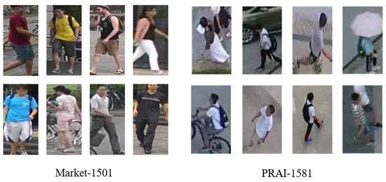
Figure 9.
Example images in the Market-1501 and PRAI-1581 datasets. Compared to the Market-1501 dataset, the PRAI-1581 dataset contains rich scale diversity, including low resolution, partial occlusion, different perspectives, person posture, and UAVs flying at different altitudes.
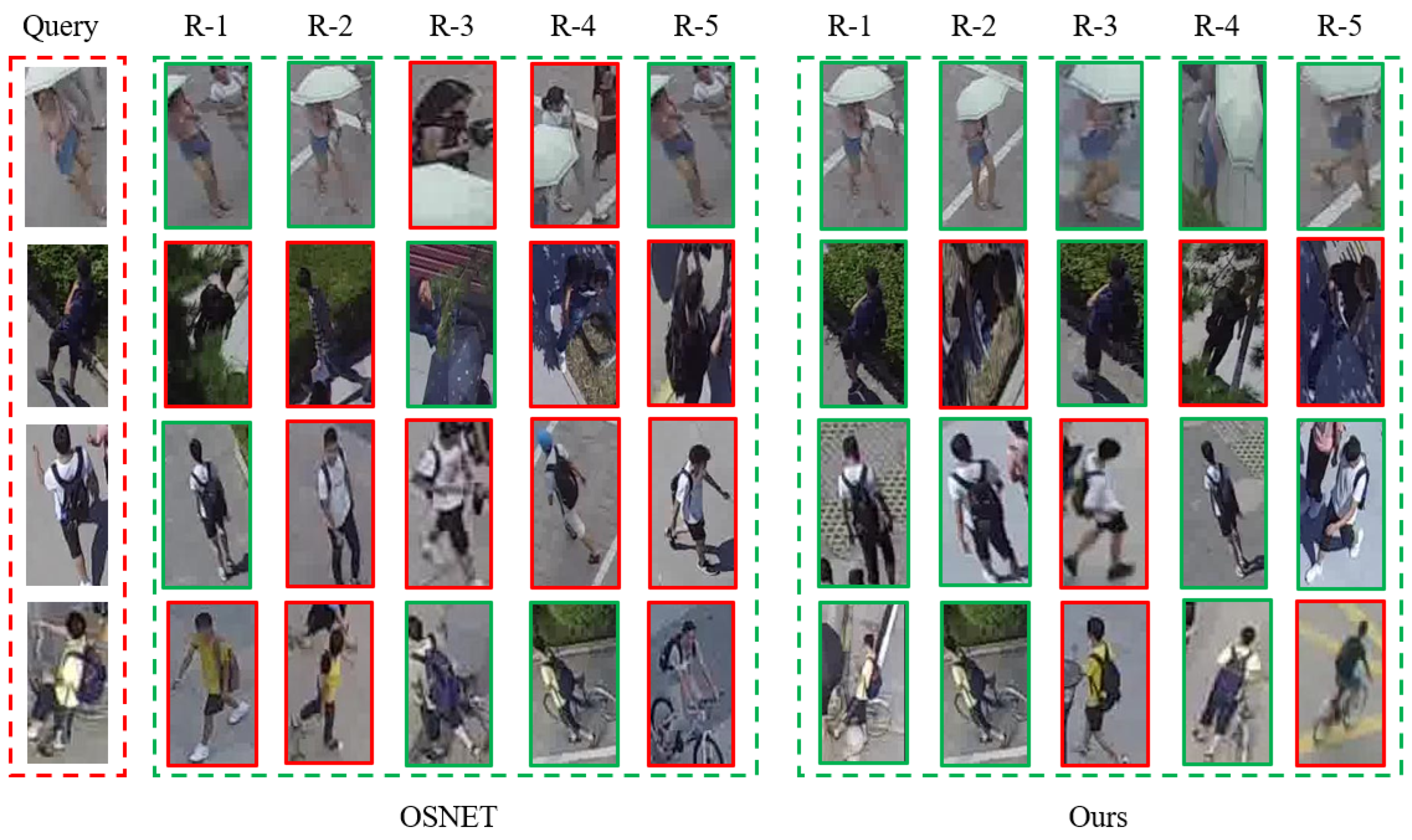
Then, we conducted supervised experiments on the PRAI-1581 to demonstrate the generalization ability of our method, as shown in Table 8. Our method achieves % in mAP and % in rank-1 accuracy on PRAI-1581, which is % higher than OSNET [54] in rank-1. The outcomes indicate that our method performs effectively, even when handling intricate datasets with authentic labels. This further validates the efficacy and generalization capabilities of our approach for person Re-ID, whether supervised or unsupervised, remote sensing images or normal images. In addition, we illustrate the search outcomes of JCL and OSNET [54] on the PRAI-1581 dataset. As shown in Figure 10, the gallery instances retrieved are indicated by green bounding boxes if they match the query instances. On the contrary, the ones denoted with red bounding boxes represent individuals with identities distinct from the query instances. The outcomes from the initial query instance suggest that, despite occasional occlusion and variations in person posture, the JCL method can accurately retrieve a person with the same ID.

Table 8.
Comparison with the Re-ID methods on PRAI-1581. ID denotes identification loss, TL denotes triplet loss, SP denotes subspace pooling. Bold indicates the best performance.
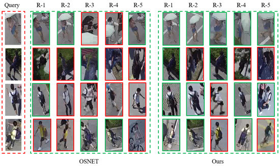
Figure 10.
Comparing the top-5 ranking lists between baseline and our method on PRAI-1581. Images with green borders indicate correct matches, while those with red borders signify incorrect matches.
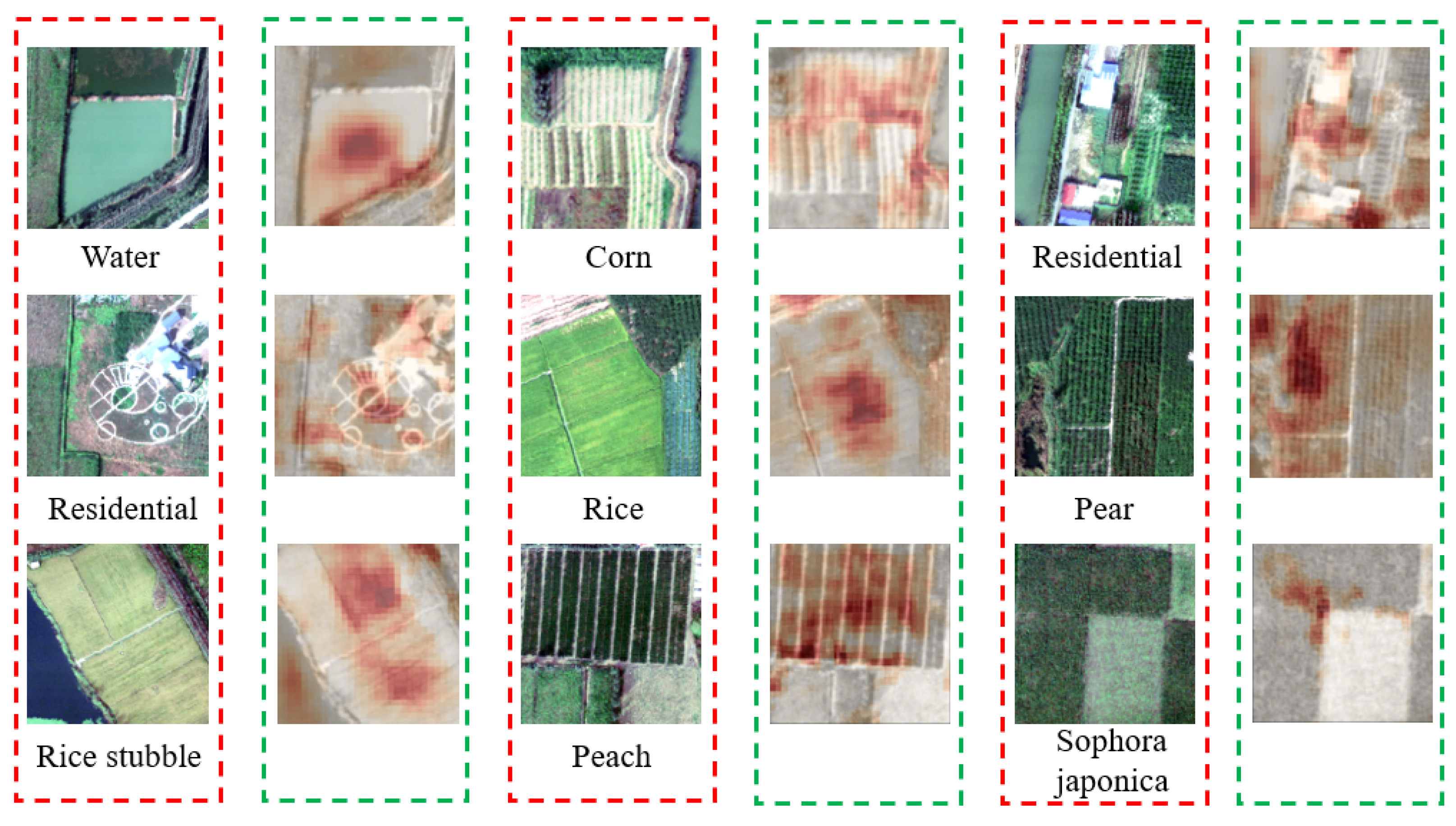
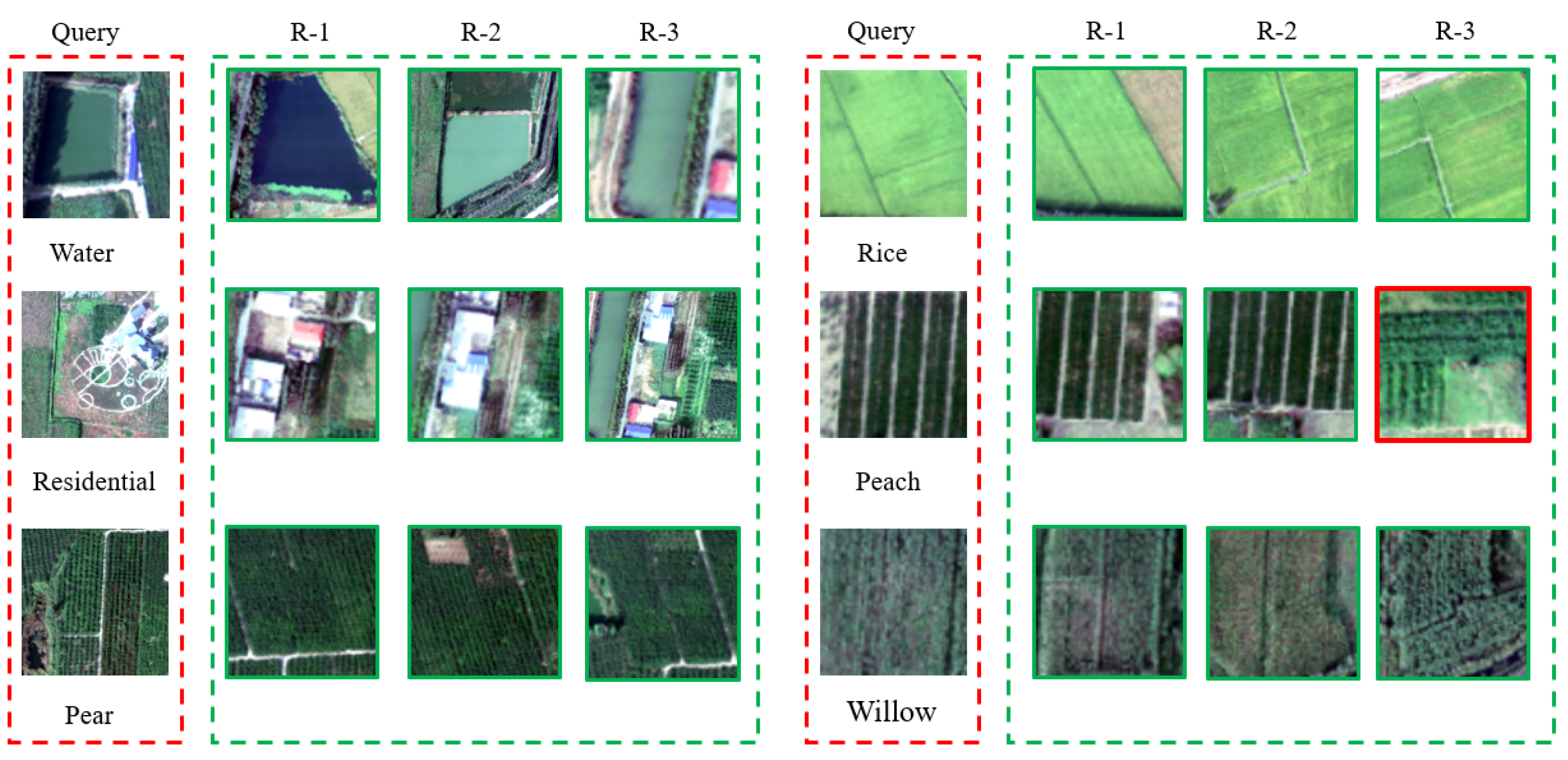
Meanwhile, we conducted experiments on the Xiongan New Area dataset. Figure 11 shows the visualization effect of our method on the Xiongan New Area dataset. It is evident that our WAM module excels in identifying the region of interest, underscoring its ability to adeptly capture crucial information within the image. As an illustration, consider the first image depicted in Figure 11. In this instance, we effectively identify and retrieve the water body segment within the image. Subsequently, we assign increased weights to facilitate the model in extracting more distinctive features. This further substantiates the effectiveness of our model, showcasing its proficiency not only in accurately detecting a person but also in demonstrating commendable generalization capabilities when identifying buildings, woodlands, and various other objects. In addition, we visualize the search results of JCL on the Xiongan New Area dataset. As shown in Figure 12, the gallery instances retrieved are indicated by green bounding boxes if they match the query instances. On the contrary, the ones denoted with red bounding boxes represent individuals with identities distinct from the query instances.
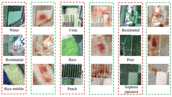
Figure 11.
Grad-CAM visualization of feature maps extracted by our model in the Xiongan New Area dataset. The red box represents the original image, and the green box represents the heatmap.
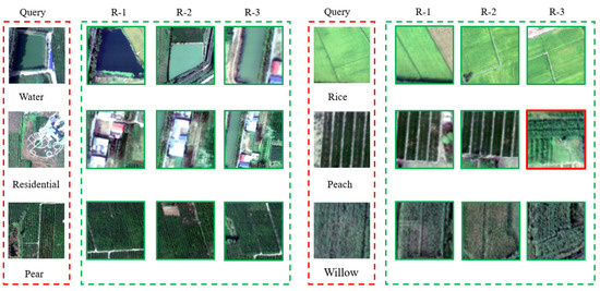
Figure 12.
Our model obtains the top-3 ranking lists for Xiongan New Area dataset. Images with green borders indicate correct matching, while images with red borders indicate incorrect matching.
5. Conclusions
In this paper, we propose a new joint contrastive learning framework designed for purely unsupervised person Re-ID. Specifically, our model takes into account both cluster and instance-level information in acquiring more discriminative features so as to achieve good recognition results. Our proposed model incorporates WAM and a cluster-filtering approach to capture more distinctive features of a person and diminish the influence of background. The experimental results demonstrate the effectiveness of our proposed method. In addition, our approach demonstrates commendable performance on remote sensing datasets, highlighting its excellence in feature extraction and model generalization ability.
As local information contributes to effective representation learning, our model has scope for further performance enhancement. In the future, we aim to integrate local information as important clues for identifying people to alleviate the adverse effects of pseudo-label noise.
Author Contributions
Conceptualization, methodology, writing, funding acquisition, and supervision, G.Z. and J.L.; software, validation, and data curation, J.L., Z.Y. and G.Z. All authors have read and agreed to the published version of the manuscript.
Funding
This research was supported by the National Natural Science Foundation of China (Grant number: 62172231, U22B2056); Natural Science Foundation of Jiangsu Province of China (Grant number: BK20220107).
Data Availability Statement
This study is available on request from the corresponding author.
Conflicts of Interest
The authors declare no conflicts of interest.
References
- Zhang, Z.; Lan, C.; Zeng, W.; Jin, X.; Chen, Z. Relation-aware global attention for person re-identification. In Proceedings of the IEEE/CVF Conference on Computer Vision and Pattern Recognition, Seattle, WA, USA, 13–19 June 2020; pp. 3186–3195. [Google Scholar]
- Chen, Y.; Zhang, G.; Lu, Y.; Wang, Z.; Zheng, Y. Tipcb: A simple but effective part-based convolutional baseline for text-based person search. Neurocomputing 2022, 494, 171–181. [Google Scholar] [CrossRef]
- Zhong, Z.; Zheng, L.; Cao, D.; Li, S. Re-ranking person re-identification with k-reciprocal encoding. In Proceedings of the IEEE Conference on Computer Vision and Pattern Recognition, Honolulu, HI, USA, 21–26 July 2017; pp. 1318–1327. [Google Scholar]
- Zhang, G.; Ge, Y.; Dong, Z.; Wang, H.; Zheng, Y.; Chen, S. Deep high-resolution representation learning for cross-resolution person re-identification. IEEE Trans. Image Process. 2021, 30, 8913–8925. [Google Scholar] [CrossRef]
- Zhang, G.; Liu, J.; Chen, Y.; Zheng, Y.; Zhang, H. Multi-biometric unified network for cloth-changing person re-identification. IEEE Trans. Image Process. 2023, 32, 4555–4566. [Google Scholar]
- Ge, Y.; Zhu, F.; Chen, D.; Zhao, R. Self-paced contrastive learning with hybrid memory for domain adaptive object re-id. Adv. Neural Inf. Process. Syst. 2020, 33, 11309–11321. [Google Scholar]
- Zhang, G.; Zhang, H.; Lin, W.; Chandran, A.K.; Jing, X. Camera contrast learning for unsupervised person re-identification. IEEE Trans. Circuits Syst. Video Technol. 2023, 33, 4096–4107. [Google Scholar] [CrossRef]
- Wang, M.; Lai, B.; Huang, J.; Gong, X.; Hua, X.S. Camera-aware proxies for unsupervised person re-identification. In Proceedings of the AAAI Conference on Artificial Intelligence, Vancouver, BC, Canada, 2–9 February 2021; Volume 35, pp. 2764–2772. [Google Scholar]
- Wang, M.; Li, J.; Lai, B.; Gong, X.; Hua, X.S. Offline-online associated camera-aware proxies for unsupervised person re-identification. IEEE Trans. Image Process. 2022, 31, 6548–6561. [Google Scholar] [CrossRef] [PubMed]
- Yang, F.; Zhong, Z.; Luo, Z.; Cai, Y.; Lin, Y.; Li, S.; Sebe, N. Joint noise-tolerant learning and meta camera shift adaptation for unsupervised person re-identification. In Proceedings of the IEEE/CVF Conference on Computer Vision and Pattern Recognition, Nashville, TN, USA, 20–25 June 2021; pp. 4855–4864. [Google Scholar]
- Wang, D.; Zhang, S. Unsupervised person re-identification via multi-label classification. In Proceedings of the IEEE/CVF Conference on Computer Vision and Pattern Recognition, Seattle, WA, USA, 13–19 June 2020; pp. 10981–10990. [Google Scholar]
- Ge, Y.; Chen, D.; Li, H. Mutual mean-teaching: Pseudo label refinery for unsupervised domain adaptation on person re-identification. arXiv 2020, arXiv:2001.01526. [Google Scholar]
- Han, J.; Li, Y.L.; Wang, S. Delving into probabilistic uncertainty for unsupervised domain adaptive person re-identification. In Proceedings of the AAAI Conference on Artificial Intelligence, Vancouver, BC, Canada, 20–27 February 2022; Volume 36, pp. 790–798. [Google Scholar]
- Gu, J.; Chen, W.; Luo, H.; Wang, F.; Li, H.; Jiang, W.; Mao, W. Multi-view evolutionary training for unsupervised domain adaptive person re-identification. IEEE Trans. Inf. Forensics Secur. 2022, 17, 344–356. [Google Scholar] [CrossRef]
- Chen, H.; Wang, Y.; Lagadec, B.; Dantcheva, A.; Bremond, F. Joint generative and contrastive learning for unsupervised person re-identification. In Proceedings of the IEEE/CVF Conference on Computer Vision and Pattern Recognition, Nashville, TN, USA, 20–25 June 2021; pp. 2004–2013. [Google Scholar]
- Chen, H.; Lagadec, B.; Bremond, F. Ice: Inter-instance contrastive encoding for unsupervised person re-identification. In Proceedings of the IEEE/CVF International Conference on Computer Vision, Montreal, BC, Canada, 11–17 October 2021; pp. 14960–14969. [Google Scholar]
- Dai, Z.; Wang, G.; Yuan, W.; Zhu, S.; Tan, P. Cluster contrast for unsupervised person re-identification. In Proceedings of the Asian Conference on Computer Vision, Macau, China, 4–8 December 2022; pp. 1142–1160. [Google Scholar]
- Lin, Y.; Dong, X.; Zheng, L.; Yan, Y.; Yang, Y. A bottom-up clustering approach to unsupervised person re-identification. In Proceedings of the AAAI Conference on Artificial Intelligence, Honolulu, HI, USA, 27 January–1 February 2019; Volume 33, pp. 8738–8745. [Google Scholar]
- Sun, H.; Li, M.; Li, C.G. Hybrid contrastive learning with cluster ensemble for unsupervised person re-identification. In Proceedings of the Asian Conference on Pattern Recognition, Jeju Island, Republic of Korea, 9–12 November 2021; pp. 532–546. [Google Scholar]
- Zhang, H.; Zhang, G.; Chen, Y.; Zheng, Y. Global relation-aware contrast learning for unsupervised person re-identification. IEEE Trans. Circuits Syst. Video Technol. 2022, 32, 8599–8610. [Google Scholar] [CrossRef]
- He, Q.; Wang, Z.; Zheng, Z.; Hu, H. Spatial and Temporal Dual-Attention for Unsupervised Person Re-Identification. IEEE Trans. Intell. Transp. Syst. 2023, 1–13. [Google Scholar] [CrossRef]
- Zhang, G.; Chen, Y.; Lin, W. Low resolution information also matters: Learning multi-resolution representations for person re-identification. In Proceedings of the International Joint Conference on Artificial Intelligence, Montreal, QC, Canada, 19–27 August 2021; pp. 1295–1301. [Google Scholar]
- Zhang, S.; Zhang, Q.; Yang, Y.; Wei, X.; Wang, P.; Jiao, B.; Zhang, Y. Person re-identification in aerial imagery. IEEE Trans. Multimedia 2020, 23, 281–291. [Google Scholar]
- Yi, C.E.N.; Zhang, L.; Zhang, X. Aerial hyperspectral remote sensing classification dataset of Xiongan New Area (Matiwan Village). Natl. Remote Sens. Bull. 2020, 24, 1299–1306. [Google Scholar]
- Deng, W.; Zheng, L.; Ye, Q.; Kang, G.; Yang, Y.; Jiao, J. Image-image domain adaptation with preserved self-similarity and domain-dissimilarity for person re-identification. In Proceedings of the IEEE Conference on Computer Vision and Pattern Recognition, Salt Lake City, UT, USA, 18–23 June 2018; pp. 994–1003. [Google Scholar]
- Zhu, J.Y.; Park, T.; Isola, P.; Efros, A.A. Unpaired image-to-image translation using cycle-consistent adversarial networks. In Proceedings of the IEEE International Conference on Computer Vision, Venice, Italy, 22–29 October 2017; pp. 2223–2232. [Google Scholar]
- Zhang, G.; Fang, W.; Zheng, Y.; Wang, R. SDBAD-Net: A Spatial Dual-Branch Attention Dehazing Network based on Meta-Former Paradigm. IEEE Trans. Circuits Syst. Video Technol. 2023, 34, 60–70. [Google Scholar]
- Wang, F.; Jiang, M.; Qian, C.; Yang, S.; Li, C.; Zhang, H.; Tang, X. Residual attention network for image classification. In Proceedings of the IEEE Conference on Computer Vision and Pattern Recognition, Honolulu, HI, USA, 21–26 July 2017; pp. 3156–3164. [Google Scholar]
- Zhang, Z.; Zhang, H.; Liu, S. Person re-identification using heterogeneous local graph attention networks. In Proceedings of the IEEE/CVF Conference on Computer Vision and Pattern Recognition, Nashville, TN, USA, 20–25 June 2021; pp. 12136–12145. [Google Scholar]
- Zhang, G.; Sun, H.; Zheng, Y.; Xia, G.; Feng, L.; Sun, Q. Optimal discriminative projection for sparse representation-based classification via bilevel optimization. IEEE Trans. Circuits Syst. Video Technol. 2019, 30, 1065–1077. [Google Scholar]
- Li, M.; Li, C.G.; Guo, J. Cluster-guided asymmetric contrastive learning for unsupervised person re-identification. IEEE Trans. Image Process. 2022, 31, 3606–3617. [Google Scholar] [CrossRef] [PubMed]
- Hong, D.; Han, Z.; Yao, J.; Gao, L.; Zhang, B.; Plaza, A.; Chanussot, J. SpectralFormer: Rethinking hyperspectral image classification with transformers. IEEE Trans. Geosci. Remote Sens. 2021, 60, 1–15. [Google Scholar] [CrossRef]
- Tao, C.; Qi, J.; Guo, M.; Zhu, Q.; Li, H. Self-supervised remote sensing feature learning: Learning paradigms, challenges, and future works. IEEE Trans. Geosci. Remote Sens. 2023, 61, 5610426. [Google Scholar] [CrossRef]
- Huang, S.; Zhang, H.; Pižurica, A. Subspace clustering for hyperspectral images via dictionary learning with adaptive regularization. IEEE Trans. Geosci. Remote Sens. 2021, 60, 5524017. [Google Scholar] [CrossRef]
- Liu, Z.; Zhong, Y.; Wang, X.; Shu, M.; Zhang, L. Unsupervised Deep Hyperspectral Video Target Tracking and High Spectral-Spatial-Temporal Resolution (H³) Benchmark Dataset. IEEE Trans. Geosci. Remote Sens. 2021, 60, 5513814. [Google Scholar] [CrossRef]
- Wang, W.; Zhao, F.; Liao, S.; Shao, L. Attentive waveblock: Complementarity-enhanced mutual networks for unsupervised domain adaptation in person re-identification and beyond. IEEE Trans. Image Process. 2022, 31, 1532–1544. [Google Scholar] [CrossRef]
- Zhang, G.; Luo, Z.; Chen, Y.; Zheng, Y.; Lin, W. Illumination unification for person re-identification. IEEE Trans. Circuits Syst. Video Technol. 2022, 32, 6766–6777. [Google Scholar] [CrossRef]
- Zheng, L.; Shen, L.; Tian, L.; Wang, S.; Wang, J.; Tian, Q. Scalable person re-identification: A benchmark. In Proceedings of the IEEE International Conference on Computer Vision, Santiago, Chile, 7–13 December 2015; pp. 1116–1124. [Google Scholar]
- Ristani, E.; Solera, F.; Zou, R.; Cucchiara, R.; Tomasi, C. Performance measures and a data set for multi-target, multi-camera tracking. In Proceedings of the European Conference on Computer Vision, Amsterdam, The Netherlands, 11–14 October 2016; pp. 17–35. [Google Scholar]
- Gray, D.; Brennan, S.; Tao, H. Evaluating appearance models for recognition, reacquisition, and tracking. In Proceedings of the IEEE International Workshop on Performance Evaluation for Tracking and Surveillance (PETS), Rio de Janeiro, Brazil, 14 October 2007; Volume 3, pp. 1–7. [Google Scholar]
- He, K.; Zhang, X.; Ren, S.; Sun, J. Deep residual learning for image recognition. In Proceedings of the IEEE Conference on Computer Vision and Pattern Recognition, Las Vegas, NV, USA, 27–30 June 2016; pp. 770–778. [Google Scholar]
- Deng, J.; Dong, W.; Socher, R.; Li, L.J.; Li, K.; Li, F. Imagenet: A large-scale hierarchical image database. In Proceedings of the 2009 IEEE Conference on Computer Vision and Pattern Recognition, Miami, FL, USA, 20–25 June 2009; pp. 248–255. [Google Scholar]
- Ioffe, S.; Szegedy, C. Batch normalization: Accelerating deep network training by reducing internal covariate shift. In Proceedings of the International Conference on Machine Learning, Lille, France, 6–11 July 2015; pp. 448–456. [Google Scholar]
- Ester, M.; Kriegel, H.P.; Sander, J.; Xu, X. A density-based algorithm for discovering clusters in large spatial databases with noise. kdd 1996, 96, 226–231. [Google Scholar]
- Li, J.; Zhang, S. Joint visual and temporal consistency for unsupervised domain adaptive person re-identification. In Proceedings of the Computer Vision—ECCV 2020: 16th European Conference, Glasgow, UK, 23–28 August 2020; pp. 483–499. [Google Scholar]
- Li, Z.; Shi, Y.; Ling, H.; Chen, J.; Wang, Q.; Zhou, F. Reliability exploration with self-ensemble learning for domain adaptive person re-identification. In Proceedings of the AAAI Conference on Artificial Intelligence, Vancouver, BC, Canada, 20–27 February 2022; Volume 36, pp. 1527–1535. [Google Scholar]
- Zeng, K.; Ning, M.; Wang, Y.; Guo, Y. Hierarchical clustering with hard-batch triplet loss for person re-identification. In Proceedings of the IEEE/CVF Conference on Computer Vision and Pattern Recognition, Seattle, WA, USA, 13–19 June 2020; pp. 13657–13665. [Google Scholar]
- Zhang, X.; Ge, Y.; Qiao, Y.; Li, H. Refining pseudo labels with clustering consensus over generations for unsupervised object re-identification. In Proceedings of the IEEE/CVF Conference on Computer Vision and Pattern Recognition, Nashville, TN, USA, 20–25 June 2021; pp. 3436–3445. [Google Scholar]
- He, T.; Shen, L.; Guo, Y.; Ding, G.; Guo, Z. Secret: Self-consistent pseudo label refinement for unsupervised domain adaptive person re-identification. In Proceedings of the AAAI Conference on Artificial Intelligence, Vancouver, BC, Canada, 20–27 February 2022; Volume 36, pp. 879–887. [Google Scholar]
- Guo, Z.; Ma, B.; Chang, H.; Chen, X. Gradual Domain Adaptation with Sample Transferability Exploitation for Person Re-Identification. In Proceedings of the 2022 IEEE International Conference on Multimedia and Expo (ICME), Taipei, Taiwan, 18–22 July 2022; pp. 1–6. [Google Scholar]
- Liu, T.; Lin, Y.; Du, B. Unsupervised person re-identification with stochastic training strategy. IEEE Trans. Image Process. 2022, 31, 4240–4250. [Google Scholar] [CrossRef] [PubMed]
- Wang, X.; Liu, M.; Wang, F.; Dai, J.; Liu, A.; Wang, Y. Relation-Preserving Feature Embedding for Unsupervised Person Re-identification. IEEE Trans. Multimedia 2023, 26, 714–723. [Google Scholar]
- Bertocco, G.; Theophilo, A.; Andaló, F.; Rocha, A. Leveraging ensembles and self-supervised learning for fully-unsupervised person re-identification and text authorship attribution. IEEE Trans. Inf. Forensics Secur. 2023, 18, 3876–3890. [Google Scholar]
- Zhou, K.; Yang, Y.; Cavallaro, A.; Xiang, T. Omni-scale feature learning for person re-identification. In Proceedings of the IEEE/CVF International Conference on Computer Vision, Seoul, Republic of Korea, 27 October–2 November 2019; pp. 3702–3712. [Google Scholar]
Disclaimer/Publisher’s Note: The statements, opinions and data contained in all publications are solely those of the individual author(s) and contributor(s) and not of MDPI and/or the editor(s). MDPI and/or the editor(s) disclaim responsibility for any injury to people or property resulting from any ideas, methods, instructions or products referred to in the content. |
© 2024 by the authors. Licensee MDPI, Basel, Switzerland. This article is an open access article distributed under the terms and conditions of the Creative Commons Attribution (CC BY) license (https://creativecommons.org/licenses/by/4.0/).

