Article

Inter-Calibration of Passive Microwave Satellite Brightness Temperature Observations between FY-3D/MWRI and GCOM-W1/AMSR2

1
Heilongjiang Eco-Meteorology Center, Heilongjiang Meteorological Bureau, Harbin 150030, China
2
Key Laboratory of Radiometric Calibration and Validation for Environmental Satellites, National Satellite Meteorological Center (National Center for Space Weather), China Meteorological Administration, Beijing 100081, China
3
Innovation Center for FengYun Meteorological Satellite (FYSIC), Beijing 100081, China
*
Author to whom correspondence should be addressed.
Remote Sens. 2024, 16(2), 424; https://doi.org/10.3390/rs16020424
Submission received: 22 December 2023 / Revised: 16 January 2024 / Accepted: 19 January 2024 / Published: 22 January 2024
(This article belongs to the Special Issue Remote Sensing Satellites Calibration and Validation)

Abstract

:
Microwave sensors possess the capacity to effectively penetrate through clouds and fog and are widely used in obtaining soil moisture, atmospheric water vapor, and surface temperature measurements. Long time-series datasets play a pivotal role in climate change studies. Unfortunately, the lifespan of operational satellites often falls short of the needs of these extensive datasets. Hence, comparing and cross-calibrating sensors with similar configurations is paramount. The Microwave Radiation Imager (MWRI) onboard Fengyun-3D (FY-3D) is the latest generation of satellite-based microwave remote sensing instruments in China, and its data quality and application prospects have attracted widespread attention. To comprehensively assess the data quality of MWRI, a comparison of the orbital brightness temperature (TB) data between FY-3D/MWRI and Global Change Observation Mission 1st-Water (GCOM-W1)/Advanced Microwave Scanning Radiometer 2 (AMSR2) is conducted, and then a calibration model is established. The results indicate a strong correlation between the two sensors, with a correlation coefficient exceeding 0.9 across all channels. The mean bias ranges from −1.5 K to 0.15 K. Notably, the bias of vertical polarization is more pronounced than that of horizontal polarization. The TB distribution patterns and temporal evolutions are highly consistent for both sensors, particularly under snow and ice. The small intercepts and close-to-1 slopes obtained during calibration further demonstrate the minor data differences between the two sensors. However, the calibration process effectively reduces the existing errors, and the calibrated FY-3D/MWRI TB data are closer to GCOM-W1/AMSR2, with a mean bias approximately equal to 0 K and a correlation coefficient exceeding 0.99. The excellent consistency of the TB data between the two sensors provides a vital data basis for retrieving surface parameters and establishing long time-series datasets.

1. Introduction

Satellite observations have become an important component in numerous studies and applications of earth science [1]. Currently, these satellite sensors possess the capability to extensively observe the earth’s surface over a wide range of frequencies and bandwidths [1]. Due to their long wavelengths (from 1 mm to 1 m), microwaves can effectively penetrate through clouds, and even snow, ice, forests, and soil in some cases [2]. Thus, microwave remote sensing stands out as the preferred technique for gaining insights into various physical variables over the earth’s surface. In addition, microwave remote sensing is invaluable in obtaining data on various hydrometeors [3]. By strategically selecting appropriate frequencies, microwave remote sensing enables the extraction of crucial information about sea ice concentrations [4,5], snow depth/water equivalent [6], soil moisture [7], and water vapor [8].
Since 1978, passive microwave satellites have played a crucial role in earth observations across a wide range of frequencies [9]. Key microwave imaging instruments include the Seasat Nimbus-G Scanning Multichannel Microwave Radiometer (SMMR), active from 1978 to 1987. It had five frequencies and ten channels, providing TB data for earth observations from 6.6 GHz to 37 GHz [10]. The Special Sensor Microwave Imager (SSM/I) has been operational since 1987, and consists of seven different microwave power radiometers operating at 19.3, 37.0, 22.2, and 85.5 GHz frequencies. The water vapor channel at 22.2 GHz employs vertical polarization, while the remaining channels employ dual polarization. The Advanced Microwave Scanning Radiometer for the Earth Observing System (AMSR-E) operated from 2002 to 2011, and was a twelve-channel and six-frequency passive microwave radiometer system, measuring TB at 6.925, 10.65, 18.7, 23.8, 36.5, and 89.0 GHz with both vertical and horizontal polarization [11]. From 2012 to the present, the Advanced Microwave Scanning Radiometer 2 (AMSR2) onboard the Global Change Observation Mission 1st-Water (GCOM-W1) satellite has continued the AMSR-E observations of water vapor, cloud liquid water, precipitation, sea surface temperature, sea surface wind speed, sea ice concentration, snow depth, and soil moisture. Additionally, two channels with a frequency of 7.3 GHz have been introduced [12,13,14,15]. The Microwave Radiation Imager (MWRI) onboard the Fengyun series satellites (FY-3A, FY-3B, FY-3C and FY-3D) has provided TB observation data since 2008. This instrument comprises five observation frequency points covering 10–89 GHz, with each frequency vertically and horizontally polarized, and ten channels [14,15,16,17]. Collectively, these instruments have facilitated earth surface observations in the frequency range from 10.65 GHz to 89 GHz. Launched in 2009, the radiometer onboard the Soil Moisture and Ocean Salinity (SMOS) mission measures L-band emissions at 1.4 GHz [18]. Additionally, from 2015 to the present, the Soil Moisture Active and Passive (SMAP) has provided another set of L-band (1.41 GHz) observation data [19,20].
Available TB data from microwave remote sensing can date back decades and can be used for climate studies [21]. However, long time series of data often come from different satellites because the lifetime of individual satellites is not long enough. The consistency of TB measurements is affected by their orbital altitude, incidence angles, sensor configuration, and observation frequencies [9]. To yield reliable datasets for surface parameters, the rigorous calibration of sensors becomes imperative. Numerous teams are presently calibrating the TB of the microwave imager to ensure the uniformity of the data. For example, the TB difference between the Global Precipitation Measurement Microwave Imager (GMI) and SMMR was compared by Favrichon et al. [9]. In addition, the calibration between AMSR-E and AMSR2 was conducted by Imaoka et al. [22]. Overlapping FY3B-MWRI sensor measurements were used for inter-calibrating TB from AMSR-E and AMSR2 by Du et al. [17]. As Chander et al. summarized, sensor inter-calibration methods can be divided into three categories: (1) simultaneous nadir overpass (SNO), (2) statistical inter-calibration (SIC), and (3) double-differencing methods [23]. The SNO method is based on the sensor’s spectral response functions and the surface characteristics. The SIC method directly compares sensor observations and uses empirical models developed from multiple (e.g., thousands) co-located observations to calibrate data from the target instrument; this method is best suited to two instruments with co-located and near-simultaneous observations. The SIC is a direct comparison of the observations of two instruments. However, it is not universally applicable due to collocation thresholds. For instruments lacking acceptable collocation thresholds, double-differencing methods come into play. These methods involve utilizing a model simulation or a third sensor as a reference, calculating the difference from the reference target separately, and finally comparing the difference to minimize the effect of different sensor configurations.
MWRI is the latest generation of China’s satellite-based microwave remote sensing instruments. At present, the comparison and calibration studies on FY-3D/MWRI TB data are few. To this end, this research focuses on utilizing the TB data from the ten channels of the MWRI sensor onboard the FY-3D satellite that are overlapping with the AMSR2 onboard the GCOM-W1/satellite. The performance of the two satellites in each channel is cross-compared and inter-calibrated, and then the calibration results are re-evaluated.
The remainder of this paper is organized as follows. Section 2 briefly describes the satellite observations used in this study and the preprocessing methods performed for the analysis. Section 3 presents the results of the cross-comparison and inter-calibration. Section 4 discusses the characteristics of the TB data from the two sensors for each channel and analyzes the effect of the inter-calibration. Finally, Section 5 summarizes the main conclusions of this study.

2. Data and Methods

2.1. Data

In this study, TB data from GCOM-W1/AMSR2 and FY-3D/MWRI are used, and their sensor configuration information and channel settings are listed in Table 1. In addition, land cover types and other data are used in this study to analyze their effects on TB, which are presented in Section 2.1.3 and Table 2.

2.1.1. FY-3D/MWRI Data

FY-3D orbits at a nominal altitude of 836 km, with an orbital inclination of 98.75°, an eccentricity less than or equal to 0.0025, an orbital period of 101.5 min, a return period of about 5.5 days, and a satellite mass of nearly 3 tons. The MWRI onboard FY-3D is one of the primary payloads, with five earth observation frequencies: 10.65 GHz, 18.7 GHz, 23.8 GHz, 36.5 GHz, and 89 GHz [24,25]. Each frequency has vertical and horizontal polarization types [24]. The total number of channels is ten. The spatial resolution of MWRI varies according to the frequency used, and the spatial resolution is distributed between 10 km and 70 km. The MWRI data used in this study are L1 (Level 1) data at 10.65 GHz, 18.7 GHz, 23.8 GHz, 36.5 GHz, and 89 GHz with horizontal and vertical polarization, and the resolution of each channel is listed in Table 1.

2.1.2. GCOM-W1/AMSR2 Data

The GCOM-W1 satellite was launched by the Japan Aerospace Exploration Agency in May 2012 [26]. Onboard GCOM-W1, the AMSR2 functions as a multi-frequency and full-power microwave radiometer [27], succeeding the AMSR-E in measuring weak microwave emissions from both the earth’s surface and atmosphere [22]. Positioned approximately 700 km above the earth, AMSR2 provides remarkably precise observations of microwave emissions and scattering intensity. Its antenna rotates every 1.5 s and acquires data over a 1450 km scanning range. This conical scanning mechanism allows AMSR2 to acquire daytime and nighttime data every two days and cover more than 99% of the earth’s surface. AMSR2 operates across seven microwave bands: 6.9 GHz, 7.3 GHz, 10.65 GHz, 18.7 GHz, 23.8 GHz, 36.5 GHz, and 89.0 GHz, and is dual-polarized for each frequency [28]. This study uses the horizontal-polarization and vertical-polarization data of L1 of GCOM-W1/AMSR2 at 10.65 GHz, 18.7 GHz, 23.8 GHz, 36.5 GHz, and 89.0 GHz.

2.1.3. Auxiliary Data

Three auxiliary datasets are used to cross-compare and calibrate the TB data. The temporal and geographical information datasets are derived from the MWRI and AMSR2 data’s auxiliary information, respectively. The land cover data are a MOD12Q1 Level 3 product with a spatial resolution of 500 m. These data are available from the following website: https://modis-land.gsfc.nasa.gov/landcover.html, accessed on 23 December 2023. To facilitate subsequent analysis, we resampled the land cover data to match the spatial resolution of the microwave TB data employed in this study. This step ensures seamless compatibility for later analysis. We also used FY-4A’s cloud detection product to filter pixels of cloud, which is provided on the website http://www.nsmc.org.cn, accessed on 24 December 2023.

2.2. Methods

2.2.1. Collocation

In this study, to ensure that the data are distributed over each season and that the sample size of the data is sufficient, as well as the efficiency of the computer operation, the orbital data from the 15th day and the end day of each month from January to December 2022 are used to analyze the consistency and inter-calibration effects of the TB observations from FY-3D/MWRI and GCOM-W1/AMSR2. As there are some differences in the spatial resolution and observation time between the two sensors, to obtain accurate information about the differences in TB observations and to ensure the validity of calibration, we need to carry out rigorous data preprocessing before cross-comparison and calibration, including spatial resolution matching, uniformity control, and noise suppression.
The orbit data of FY-3D/MWRI and GCOM-W1/AMSR2 are firstly projected onto the Equal-Area Scalable Earth Grid (EASE-GRID) to unify the spatial resolutions of the TB observations from the two sensors to 25 km. After the spatial resolution of the TB data is unified, the TB values with the same rows and columns can be extracted to ensure spatial consistency in the process of data pair matching. Simultaneously, we select the corresponding track data with a time interval of less than 60 min to ensure the observation time of the TB values of the two sensors is consistent. After confirming the consistency of the spatial resolution and observation time, we screen the effective pixels further:
  • Because the two sensors are observed at different times and clouds vary significantly, we use the FY-4A’s cloud detection product to remove pixels that may be clouds to ensure the accuracy of the obtained two-sensor agreement.
  • The data from ocean-covered pixels are removed in this study because sea surface roughness and foam significantly impact the TB observations of different sensors.
  • Due to the low spatial resolution of passive microwave remote sensing, it is easy to produce mixed pixels. The TB observation of mixed pixels has a more significant impact on the difference analysis of the two sensors. In this study, the land cover data at a 500 m spatial resolution are resampled onto a 25 km EASE grid, and the homogeneous and mixed pixels after resampling are distinguished. Then, based on the spatial-temporal matching of the sensors, the resampled land cover data are used to filter the homogeneous subsurface to reduce the interference of mixed image elements.
Figure 1 shows the distribution of the final data used in this study.

2.2.2. Error Metrics

The TB data of FY-3D/MWRI and GCOM-W1/AMSR2 are evaluated through three error metrics:
Pearson correlation coefficient (R): this metric is employed to assess the consistency of TB values between the two sensors.
Bias (mean bias): the difference of TB values between FY-3D/MWRI and GCOM-W1/AMSR2 is measured using the mean bias (bias) [29].
Root mean square error (RMSE): the RMSE is interpreted as the standard deviation of the random error, and is used to assess the dispersion [19,30].
The specific formulas for calculating these three metrics are as follows:
R = i = 1 n ( TB MWRI i TB MWRI ¯ ) TB AMSR 2 i TB AMSR 2 ¯ i = 1 n ( TB MWRI i TB MWRI ¯ ) 2 i = 1 n ( TB AMSR 2 i TB AMSR 2 ¯ ) 2
BIAS = TB MWRI ¯ TB AMSR 2 ¯
RMSE = 1 n i = 1 n ( TB MWRI i TB AMSR 2 i ) 2
where TBMWRI and TBAMSR2 denote the TB data for each channel of FY-3D/MWRI and GCOM-W1/AMSR2, respectively. The variable n is the number of data pairs compared between the two sensors. The overbar denotes the average of the data.

3. Results and Analysis

3.1. Overall Assessment

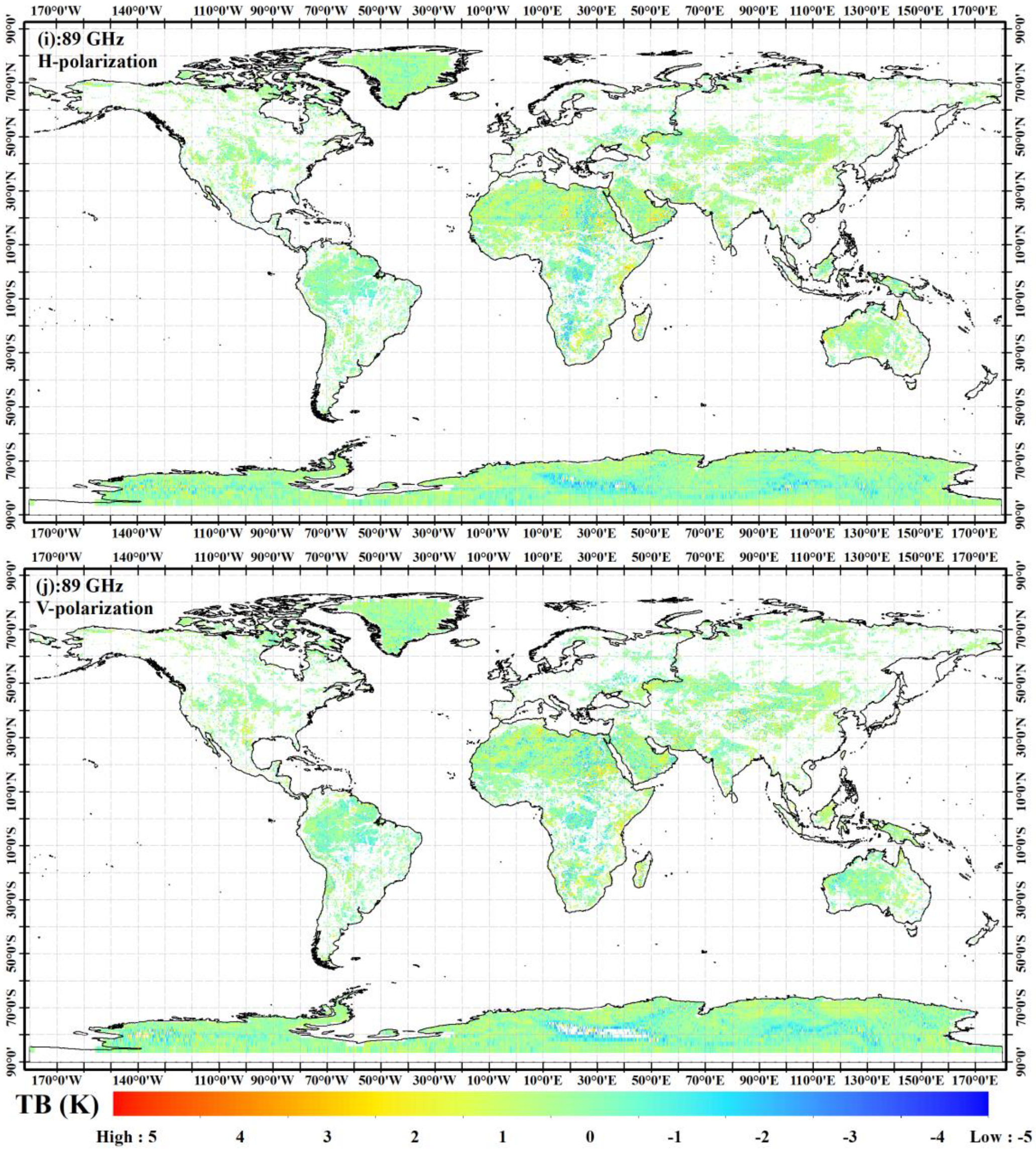
Evaluations of the FY-3D/MWRI and GCOM-W1/AMSR2 TB over homogeneous pixels have helped investigate the characteristics and stability of the data from both sensors at 10.65–89 GHz (H- and V-polarization). In this study, comparisons between FY-3D/MWRI and GCOM-W1/AMSR2 data are conducted globally to obtain a complete perspective on the total land mass. Moreover, to perform the evaluations over a global range for one year, we calculated the difference between the orbital mean data on the 15th day and the last day of each month from January to December, i.e., mean [FY-3D/MWRI]-mean [GCOM-W1/AMSR2] in each grid cell for the corresponding channels, using the 25 km EASE-gridded data from both sensors. Figure 2a–j illustrate these annual mean differences at 10.65, 18.7, 23.8, 36.5, and 89 GHz (H- and V-polarization). On each channel, the difference between the annual means (Figure 2) is generally within ±2 K globally for both H- and V-polarization data, indicating relatively good agreement. Most of the annual mean difference is very small, ranging from −1 K to 0 K (Figure 2), possibly due to the difference in incident angles and surface temperature during the sensor overpass times. In addition, there are more significant differences in some areas (e.g., North America), primarily due to radio frequency interferences (RFIs) in both H- and V-polarization images. Figure 2 also shows higher differences that are not RFI along the coastlines, and these are because of the contamination (due to water) of the large footprints of both sensors in different geometries (e.g., viewing angle and sidelobes). The results are consistent with the findings of [1,31]. However, all channels have smaller differences, indicating good agreement over the global landmass of FY-3D/MWRI and GCOM-W1/AMSR2.
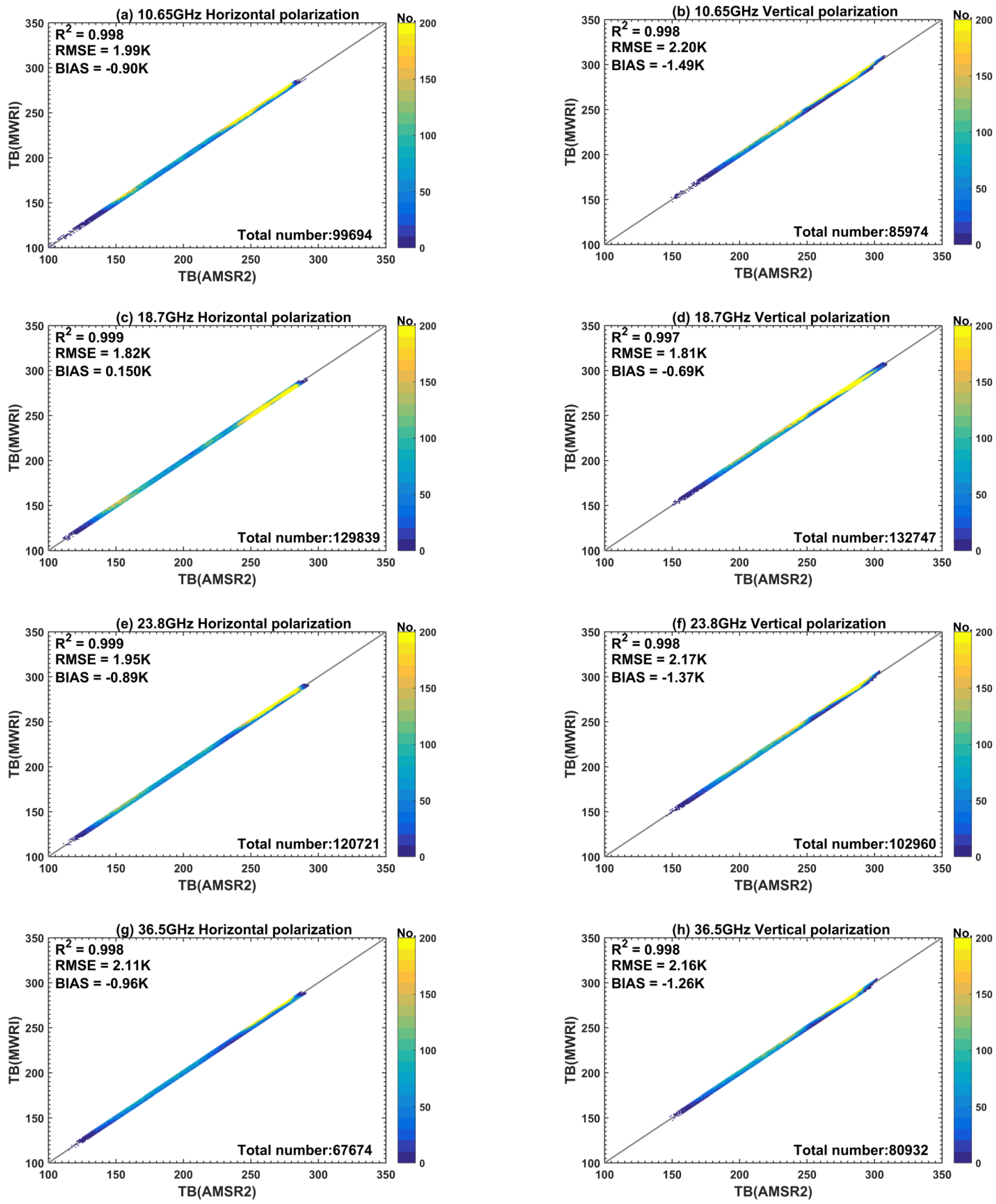
In this study, a comparison of the data from the two sensors has also been carried out to investigate the consistency of the FY-3D/MWRI and GCOM-W1/AMSR2 data (Figure 3), where the dots represent the number of data point pairs with eligible matches. The density scatter plot vividly displays a tight cluster of matched points, highlighting the data’s high concentration. Notably, the observations from both sensors exhibit an exceptionally strong correlation, with an R2 value exceeding 0.99. This correlation underscores the near identity of the data provided by the two sensors. However, discernible disparities exist when considering various polarization modes. The bias of vertical polarization is larger than that of horizontal polarization for each frequency. In addition, the correlation coefficients of the two sensors are higher for horizontal polarization. The wavelengths 18.7 GHz and 89 GHz have approximately equal RMSEs for horizontal and vertical polarization. For other frequencies, the RMSE values are consistently smaller for horizontal polarization. In summary, the differences in horizontal polarization are smaller than in vertical polarization for both sensors at all frequencies.
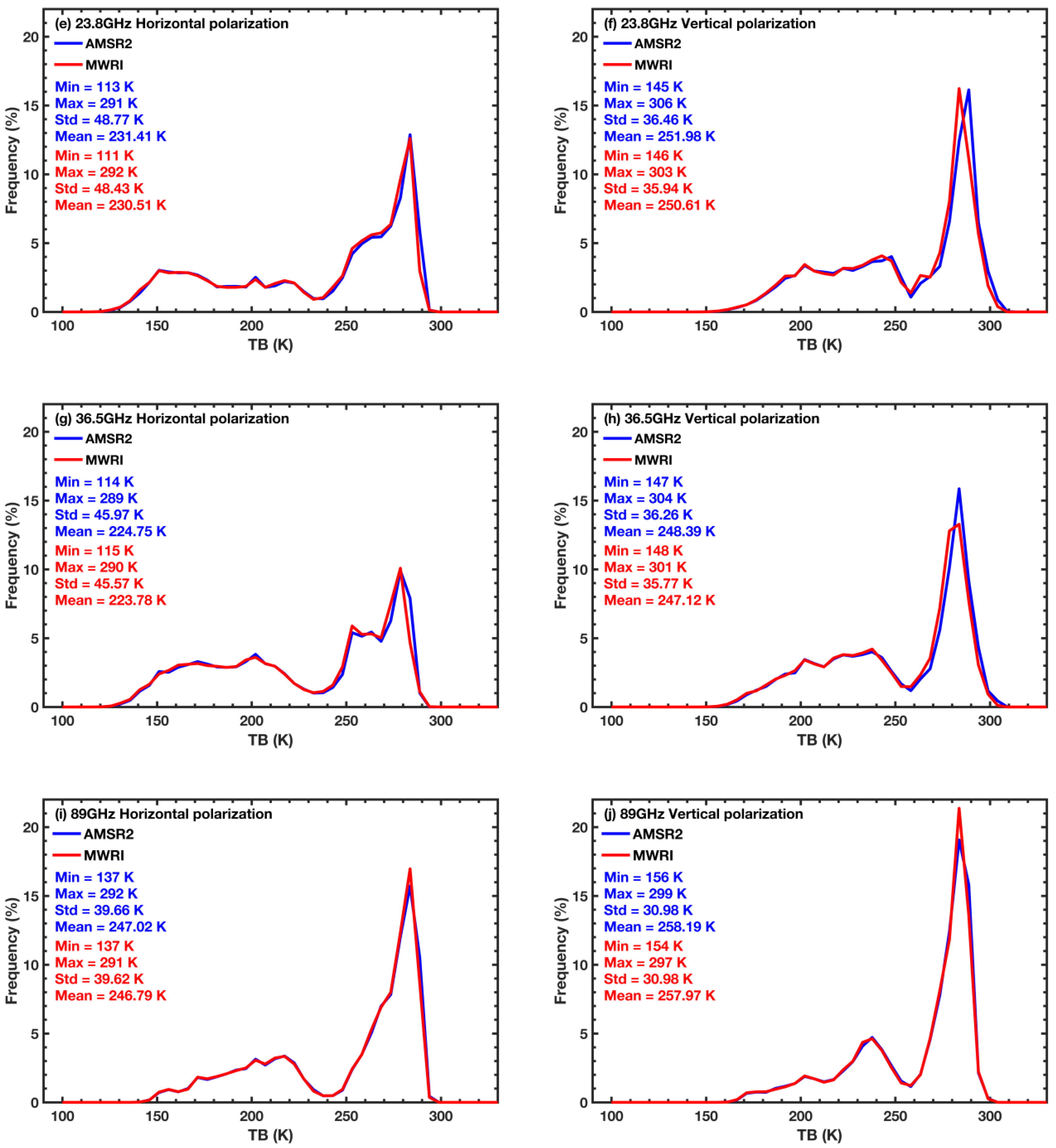
Compared with GCOM-W1/AMSR2, FY-3D/MWRI is almost the same in its channel setting except for the absence of the 6.9 GHz band. This study primarily focuses on analyzing the TB data from the ten overlapping channels. Figure 4a–j present the frequency statistical results for these ten channels of FY-3D/MWRI and GCOM-W1/AMSR2. This study also computes the maximum, minimum, average, and standard deviation of TB for each channel within the study area for a more precise comparison. The results reveal that the TB data from each channel from both sensors predominantly fall within the 100 to 320 K range. The standard deviation ranges from 30 to 50 K, and the average TB is between 200 and 250 K. The TB frequency percentages of the two sensors show a similar dynamic distribution and a relatively consistent trend. In Figure 4, for the low-frequency channel, the brightness temperatures for both sensors are distributed between low and high values. However, as the frequency increases, more and more of the brightness temperature data are distributed in the high-value region, with 89 GHz being the most pronounced, where both horizontal and vertical polarization show peaks in the high-value region (approximately 280 K). This phenomenon is attributed to more energy being available at higher frequencies than at lower frequencies, and as such the resolution is greater at higher frequencies than at lower frequencies.
Although the TB distributions of the two sensors are consistent for each channel, there are still some differences. To compare the observations made by the two sensors, the maximum, minimum, and mean values of the TB data from each channel and their standard deviations (STDs) are statistically calculated, and the results are shown in Table 3. In particular, the difference in standard deviation (∆std = std(FY-3D/MWRI) − std(GCOM-W1/AMSR2)) and mean (∆mean = mean(FY-3D/MWRI) − mean(GCOM-W1/AMSR2)) is compared. At 10.65 GHz, the differences in standard deviation for both horizontal polarization and vertical polarization are below 0 K. This discrepancy leads to a slightly narrower range. Moreover, the mean TB value of GCOM-W1/AMSR2 exceeds that of FY-3D/MWRI, indicating systematically smaller TB values for FY-3D/MWRI dual polarizations at 10.65 GHz. At 18.7 GHz, the mean TB values of the dual polarizations for FY-3D/MWRI are either larger or approximately the same as those of GCOM-W1/AMSR2. The differences in standard deviation for horizontal polarization are above 0 K. In contrast, vertical polarization is below 0 K. This discrepancy leads to a slightly wider value range of horizontally polarized FY-3D/MWRI. In comparison, vertically polarized FY-3D/MWRI exhibits a slightly narrower range. The mean TB values for dual polarizations at 23.8 GHz, 36.5 GHz, and 89 GHz are similar to that at 10.65 GHz, with the difference between the mean values below 0 K and standard deviations below 0 K. This indicates that the FY-3D/MWRI dual polarizations in most of these channels are systematically smaller but with a slightly narrower range.
Additionally, the frequency distribution curves of TB have some shifts in some channels. Notably, the 89 GHz channel shows a smaller shift, implying a better agreement between FY-3D/MWRI and GCOM-W1/AMSR2 at this frequency. However, in other channels, the TB frequency distribution of FY-3D/MWRI displays a leftward shift compared to GCOM-W1/AMSR2, indicating that the FY-3D/MWRI observations are lower than those of GCOM-W1/AMSR2, and this conclusion is consistent with the above findings. The shifts in frequency distributions are variable across different TB ranges, with most channels showing significant shifts in the middle range of TB variations. In contrast, the frequency distributions are highly consistent at both ends of the variation range. This phenomenon is linked to the sample size and is analyzed later.
The previous analysis indicates that the observed values of the two sensors are generally close to each other, and the TB of FY-3D/MWRI is smaller than that of GCOM-W1/AMSR2 in general. However, given that these instruments might respond differently to the TB of different targets, we conducted a brief analysis by categorizing all the TB values into 12 segments, with a TB interval of 20 K. The objective is to discern the differences between the two sensors within different TB intervals. Figure 5 shows the distribution of the matching pixels’ total number, R, RMSE, and bias for FY-3D/MWRI and GCOM-W1/AMSR2 in different TB segments. As can be seen, the TB data of both sensors across ten channels predominantly fall within the range of 120–300 K. The range of the vertical polarization is smaller than that of the horizontal polarization. The TB values of vertical polarization are higher than those of horizontal polarization, and are mainly distributed in the 160–300 K range. The R2 between the two sensors varies with the change of TB. Disregarding the statistically anomalous phenomena at individual intervals caused by the small sample size, the correlation coefficients display a single-peak pattern. Specifically, the correlation coefficients increase with TB for the TB data below 280 K. The peak is within the 260–280 K interval and the correlation coefficients decrease in the 280–300 K range. According to the RMSE distributions for both sensors across different TB intervals in Figure 5, the RMSE shows a slight variation. With the increase in TB, the RMSE decreases first and then increases. Additionally, the RMSE varies little in each channel and each TB interval, with a distribution range of 1.5–2.25 K.
Unlike RMSE, the bias of the two sensors varies significantly for different channels and TB intervals. The bias is mainly in the negative range, with the individual channels having a positive bias at the TB intervals greater than 280 K. This pattern is consistent with Figure 4, reinforcing the finding that FY-3D/MWRI TB values are generally smaller than those of GCOM-W1/AMSR2. Furthermore, Figure 5 highlights that the bias in each TB interval ranges from −2.5 K to 1.5 K. For TB data in the 200–240 K range, the average bias remains relatively small (−1 K to 0 K). In contrast, more significant biases are observed for the TBs below 160 K and above 260 K, which may be related to the small amount of data in the corresponding intervals and the presence of outlier interference.
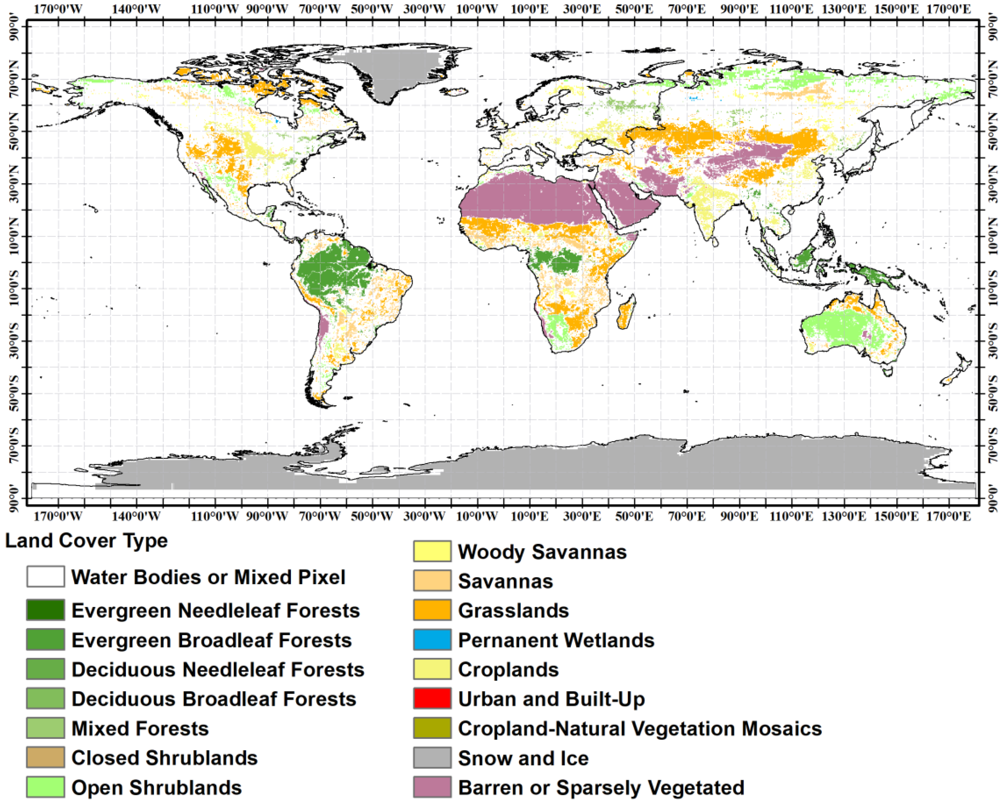
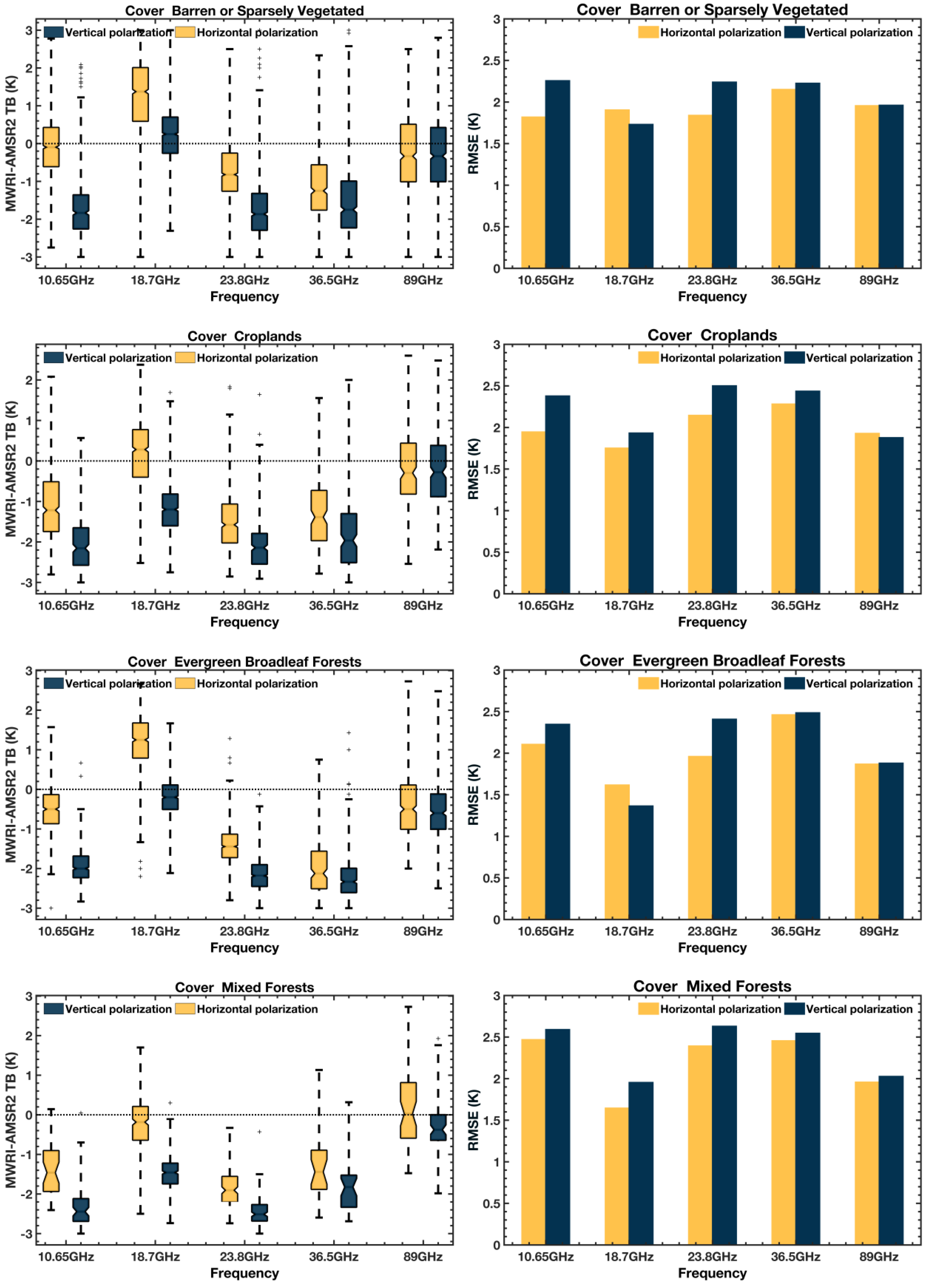
An analysis of land cover data was conducted to explore the impact of different surface types on the consistency of FY-3D/MWRI and GCOM-W1/AMSR2 data. Mixed pixels were removed during previous data processing, and Figure 6 shows the distribution of land cover types for homogeneous pixels. Nine surface types were selected for further analysis because the other surface types provided less data coverage for statistical study. The surface types analyzed in this study included barren or sparsely vegetated lands, cropland, broadleaf evergreen forest, mixed forest, grassland, open shrubland, savannah, woody savannah, and snow and ice.
The results are shown in Figure 7. When considering the “barren or sparsely vegetated” surface type, the bias of TB data towards dual polarization at 18.7 GHz consistently exhibits positive values. Notably, the biases are larger for horizontal polarization than for vertical polarization. The situation is the opposite for other frequencies, with the most negative biases seeing more significant bias for vertical polarization. This bias pattern is mirrored in the RMSE results. Moreover, as the frequency increases, the bias for both sensors approaches 0 K for dual polarizations, and the biases and RMSEs are closer between the two polarizations. For the “croplands” surface type, the TB deviation for horizontal polarization is less than the TB deviation for vertical polarization. At all frequencies, the RMSE for horizontal polarization is consistently less than 2.5 K and is smaller than or approximately equal to the RMSE for vertical polarization. For surface types of “evergreen broadleaf forests”, “grasslands”, “savannas”, and “woody savannas”, the behavior of the TB data for both sensors are consistent with the situation of the “barren or sparsely vegetated” surface type across all frequency bands. When the surface type is “mixed forests” and “open shrublands”, the TB bias of both sensors performs the same as when the surface type is “croplands”. In the surface type of “open shrublands”, the RMSE values are essentially equal across both horizontal and vertical polarization. When the surface type is “snow or ice”, the performance of TB values is quite different from those of other surface types: the two sensors show the smallest bias (close to 0 K) and the smallest RMSE (close to 2 K) of all surface types. Overall, the RMSEs between the two sensors are the smallest under the land cover of “snow or ice”, followed by “barren or sparsely vegetated” land, “grasslands”, and “open shrublands”. In comparison, the RMSEs between the two sensors are the most pronounced under forests and savannas, especially “mixed forests” and “woody savannas”.
According to the difference analysis of the two sensors over various surface types, the difference in TB between the two sensors is very significant under forests and savannas. Conversely, under snow and ice, the two sensors agree well. This could be attributed to the mix of image elements. Although we selected pure pixels of the TB data as our experimental data, ensuring homogeneity within the pixel is challenging due to the low spatial resolution of the TB data of the two sensors, which is 25 KM. Overall, the difference between the two sensors is closely linked to the pixel selection. If we eliminate mixed pixels from the analysis, the difference between the two sensors would likely be reduced. Furthermore, the differences in incidence angle could also be why the consistency of the two sensors is different across different surface types.

3.2. Inter-Calibration Models and Their Evaluation

Based on the analysis above, the TB bias between FY-3D/MWRI and GCOM-W1/AMSR2 ranges from −3 to 3 K. Although the bias is approximately 0, it is still non-negligible. We used a least squares linear model to conduct inter-calibration to facilitate the acquisition of long time-series data from GCOM-W1/AMSR2 and FY-3D/MWRI. The mathematical formulas for the least squares method are given in Equations (4) and (5). The results of the intercepts and slopes are listed in Table 4. As can be seen, the slopes for each channel range from 0.99 to 1.014, demonstrating a proximity to 1. However, the slopes of horizontal polarization are consistently closer to 1 than those of vertical polarization across all frequencies. Regarding the intercept of each channel, the intercepts of horizontal polarization span from −0.8 to 1.3, while those of vertical polarization range from −2.1 to 2.3. Notably, the horizontal polarization intercept remains smaller than that of vertical polarization at all frequencies. Combining the slopes and intercepts of each band makes it evident that the TB observations of FY-3D/MWRI and GCOM-W1/AMSR2 are generally closely aligned. However, disparities emerge when considering polarization modes, with vertical polarization showing more significant differences than horizontal polarization. Utilizing the equations in Table 5, it becomes feasible to recalibrate FY-3D/MWRI data to align with GCOM-W1/AMSR2. This recalibration effectively narrows the observational difference between the two sensors and ameliorates the issue of product inconsistency that may arise when transferring the retrieval algorithm from GCOM-W1/AMSR2 to FY-3D/MWRI. The effectiveness of this recalibration is assessed by evaluating the difference between the calibrated FY-3D/MWRI TB and GCOM-W1/AMSR2 TB using the R2, RMSE, and bias presented in Table 5. As can be seen, the values of R2 for the recalibrated FY-3D/MWRI and GCOM-W1/AMSR2 data range from 0.996 to 0.999. The recalibrated data also exhibit an RMSE consistently below 2 K, with bias values approximating 0 K. In essence, the calibrated FY-3D/MWRI data achieve a high level of agreement with GCOM-W1/AMSR2. This recalibration process harmonizes the TB data between the two sensors and mitigates the challenge of inconsistent product outcomes arising from data discrepancies.
a = i = 1 n ( TB AMSR 2 i TB AMSR 2 ¯ ) TB MWRI i TB MWRI ¯ i = 1 n ( TB AMSR 2 i TB AMSR 2 ¯ ) 2
b = TB MWRI ¯ a ×   TB AMSR 2 ¯
where TBMWRI and TBAMSR2 denote the TB data for each channel of FY-3D/MWRI and GCOM-W1/AMSR2, respectively. The variable n is the number of data pairs compared between the two sensors. The overbar denotes the average of the data. The variables a and b represent the slope and intercept of the regression equation, respectively.

4. Validation and Discussion

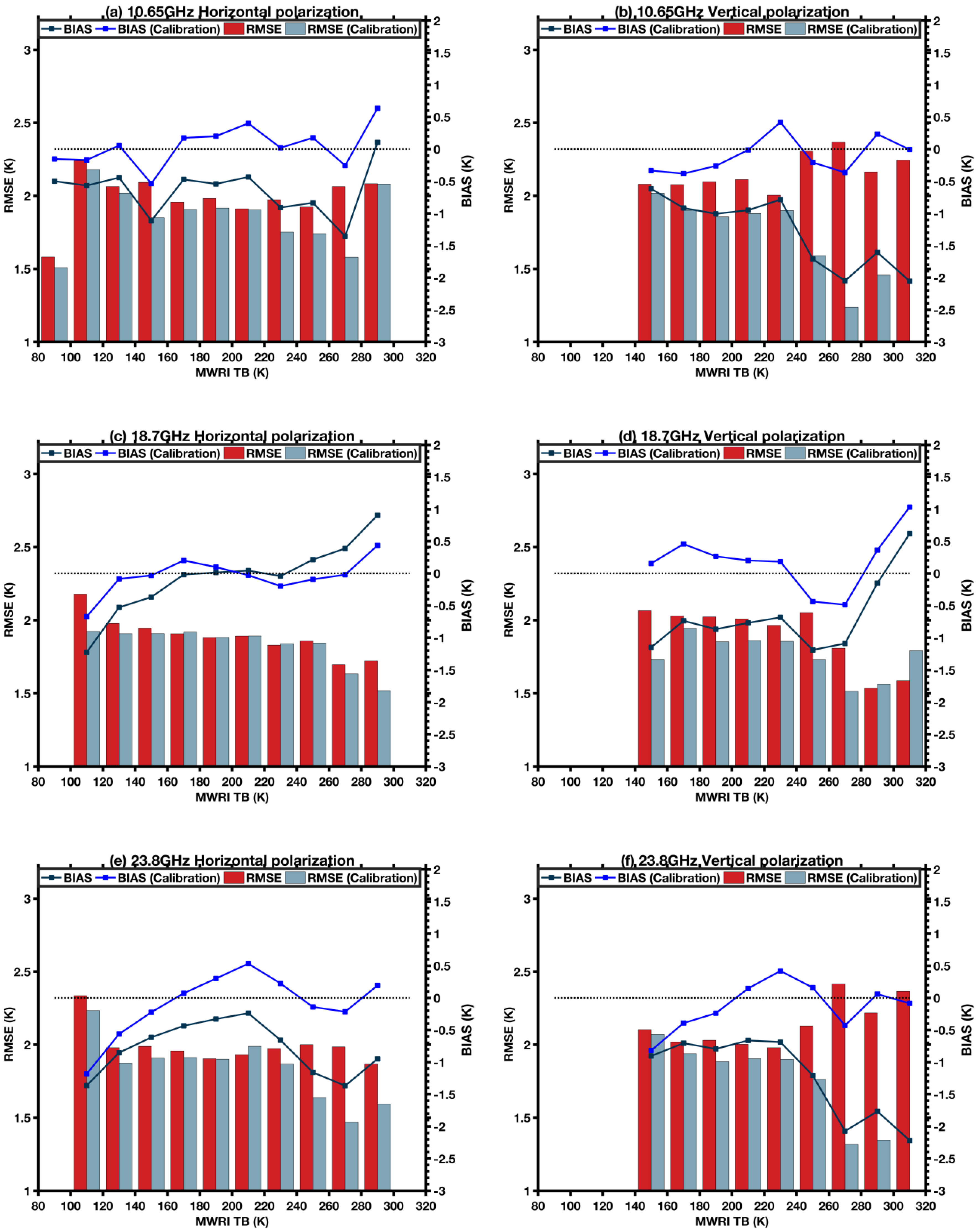
A calibration process employing a least-squares linear model is implemented to enhance the consistency and identify the differences between the two sensors. This calibration is applied to FY-3D/MWRI TB values, and the results can be compared with other TB observations. However, good agreement with this sensor is expected since the inter-calibration is from GCOM-W1/AMSR2. To further validate the effectiveness of the inter-calibration, Figure 8 illustrates a comparative analysis between the calibrated FY-3D/MWRI TB observations and those from GCOM-W1/AMSR2. The results demonstrate a close correspondence between the TB values of the calibrated FY-3D/MWRI and those of GCOM-W1/AMSR2 across all TB intervals. Nevertheless, despite the improved alignment of calibrated FY-3D/MWRI TB data with GCOM-W1/AMSR2, the calibration effect was unsatisfactory for some TB intervals, especially in the range of TBs greater than 280 K. For example, within the 280–300 K region, the bias and RMSE of the calibrated FY-3D/MWRI TB and GCOM-W1/AMSR2 data for horizontal polarization at 10.65 GHz were increased. In conjunction with the insights from Figure 5, this observation underscores that the limited sample size primarily contributes to significant TB errors in some TB intervals. Considering these realities, it is noteworthy that the alignment between the calibrated FY-3D/MWRI and GCOM-W1/AMSR2 data is significantly enhanced compared with the original FY-3D/MWRI results. These results emphasize the concurrence between GCOM-W1/AMSR2 and the inter-calibrated FY-3D/MWRI data.

5. Conclusions

Based on the similarity of the instrument parameters and channels between FY-3D/MWRI and GCOM-W1/AMSR2, as well as the reliability of GCOM-W1/AMSR2 TB data, this study conducted a comparative analysis of the orbital data from both sensors. This analysis employed statistical methods to explore and compare various aspects of the data, including their frequency, polarization mode, distribution of TB values, and land cover type.
The results indicate a strong correlation (R > 0.9) between the observed values from FY-3D/MWRI and GCOM-W1/AMSR2, with bias ranging from −1.5 K and 0.15 K. Across all channels, FY-3D/MWRI TB values are consistently slightly lower than those of GCOM-W1/AMSR2. The TB distributions of both sensors exhibit substantial similarity, and their temporal trends are also similar. Comparing the TB data from horizontal and vertical polarizations, the difference is generally smaller with horizontal rather than vertical polarization. A noteworthy pattern emerges upon assessing the impact of varying TB intervals on the bias: the difference between the two sensors initially decreases and then increases with TB values. Additionally, a compelling observation is made when examining TB data across diverse land cover types. The two sensors display their highest consistency over the surface type of snow and ice. The calibrated model, derived via the least squares approach, featured a slope nearly equal to 1 and an exceedingly minimal intercept. This outcome further underscores the remarkable proximity of FY-3D/MWRI and GCOM-W1/AMSR2 TB observations. Despite the robust correlation between the sensors, it remains vital to account for the existing bias, especially for algorithm transplantation and product utilization. To minimize the TB difference between FY-3D/MWRI and GCOM-W1/AMSR2, a meticulous calibration of FY-3D/MWRI TB was undertaken. After examination, the calibrated FY-3D/MWRI data demonstrate an outstanding alignment with GCOM-W1/AMSR2, showcasing a bias nearing 0 K and an R2 value exceeding 0.99. The calibrated data effectively minimized the observational differences between the two sensors and ameliorated the problem of product inconsistencies when transferring retrieval algorithms from GOOS-W1/AMSR2 to FY-3D/MWRI. The excellent consistency of the TB data from the two sensors after inter-calibration provides a vital data base for retrieving surface parameters and building long time-series datasets.
In this study, we diligently screened data with a transit time difference of less than 1 h. Furthermore, we examined the differences between the two sensors across different land cover types. However, despite the relative similarity in sensor parameters between FY-3D/MWRI and GCOM-W1/AMSR2, disparities in raw resolution and observation angle still exist. Consequently, it becomes imperative to consider a broader range of factors in future cross-calibration research. In addition, we only performed the calibration of FY-3D/MWRI and GCOM-W1/AMSR2. In the future, this methodology can be extended to other microwave sensors. The results of this study can also provide a basis for the study of land–air interactions and climate change.

Author Contributions

All authors contributed significantly to this manuscript. Specific contributions include data collection, Z.X. and S.W.; data analysis, Z.X. and R.S.; methodology, Z.X., J.S. and J.C.; manuscript preparation, Z.X., R.S and J.C. All authors have read and agreed to the published version of the manuscript.

Funding

The research was supported by the National Key R&D Program of China [Grant Number 2021YFC3000300].

Data Availability Statement

No new data were created or analyzed in this study. Data sharing is not applicable to this article.

Conflicts of Interest

The authors declare no conflicts of interest.

References

  1. Das, N.N.; Colliander, A.; Chan, S.K.; Njoku, E.G.; Li, L. Intercomparisons of Brightness Temperature Observations over Land from AMSR-E and WindSat. IEEE Trans. Geosci. Remote Sens. 2013, 52, 452–464. [Google Scholar] [CrossRef]
  2. Dai, L.; Che, T. Cross-platform calibration of SMMR, SSM/I and AMSR-E passive microwave brightness temperature. In Proceedings of the Sixth International Symposium on Digital Earth, Beijing, China, 9–12 September 2009; Volume 7841, pp. 45–54. [Google Scholar] [CrossRef]
  3. Gorbunov, M.E.; Kutuza, B.G. Cosmos-243 as the Starting Point for the Development of Microwave Radiometry Methods of the Earth’s Atmosphere and Surface. Izv. Atmos. Ocean. Phys. 2018, 54, 275–281. [Google Scholar] [CrossRef]
  4. Comiso, J.C.; Sullivan, C.W. Satellite microwave and in situ observations of the Weddell Sea ice cover and its marginal ice zone. J. Geophys. Res. Ocean. 1986, 91, 9663–9681. [Google Scholar] [CrossRef]
  5. Comiso, J.C.; Cavalieri, D.J.; Parkinson, C.L.; Gloersen, P. Passive microwave algorithms for sea ice concentration: A comparison of two techniques. Remote Sens. Environ. 1997, 60, 357–384. [Google Scholar] [CrossRef]
  6. Goodison, B.E.; Walker, A.E. Use of snow cover derived from satellite passive microwave data as an indicator of climate change. Ann. Glaciol. 1993, 17, 137–142. [Google Scholar] [CrossRef]
  7. Jackson, T.J. Soil moisture estimation using special satellite microwave/imager satellite data over a grassland region. Water Resour. Res. 1997, 33, 1475–1484. [Google Scholar] [CrossRef]
  8. Bauer, P.; Schluessel, P. Rainfall, total water, ice water, and water vapor over sea from polarized microwave simulations and Special Sensor Microwave/Imager data. J. Geophys. Res. Atmos. 1993, 98, 20737–20759. [Google Scholar] [CrossRef]
  9. Favrichon, S.; Prigent, C.; Jiménez, C. Inter-calibrating SMMR brightness temperatures over continental surfaces. Atmos. Meas. Tech. 2020, 13, 5481–5490. [Google Scholar] [CrossRef]
  10. Njoku, E.G.; Stacey, J.M.; Barath, F.T. The Seasat scanning multichannel microwave radiometer (SMMR): Instrument description and performance. IEEE J. Ocean. Eng. 1980, 5, 100–115. [Google Scholar] [CrossRef]
  11. Kawanishi, T. The Advanced Microwave Scanning Radiometer for the Earth Observing System (AMSR-E), NASDA’s contribution to the EOS for global energy and water cycle studies. Geosci. Remote Sens. IEEE Trans. 2003, 41, 184–194. [Google Scholar] [CrossRef]
  12. Imaoka, K.; Kachi, M.; Fujii, H.; Murakami, H.; Hori, M.; Ono, A.; Igarashi, T.; Nakagawa, K.; Oki, T.; Honda, Y.; et al. Global Change Observation Mission (GCOM) for Monitoring Carbon, Water Cycles, and Climate Change. Proc. IEEE 2010, 98, 717–734. [Google Scholar] [CrossRef]
  13. Beck, H.E.; Pan, M.; Miralles, D.G.; Reichle, R.H.; Wood, E.F. Evaluation of 18 satellite- and model-based soil moisture products using in situ measurements from 826 sensors. Hydrol. Earth Syst. Sci. 2021, 25, 17–40. [Google Scholar] [CrossRef]
  14. Wu, S.; Chen, J. Instrument performance and cross calibration of FY-3C MWRI. In Proceedings of the IGARSS 2016—2016 IEEE International Geoscience and Remote Sensing Symposium, Beijing, China, 10–15 July 2016; pp. 388–391. [Google Scholar] [CrossRef]
  15. Yang, J.; Jiang, L.; Luojus, K.; Lemmetyinen, J.; Takala, M. Assessing the Performances of FY-3D/MWRI and DMSP SSMIS in GlobSnow-2 Assimilation System for SWE Estimation. In Proceedings of the IGARSS 2020—2020 IEEE International Geoscience and Remote Sensing Symposium, Waikoloa, HI, USA, 26 September–2 October 2020; pp. 2938–2941. [Google Scholar] [CrossRef]
  16. Lu, Q.; Bell, W.; Bauer, P.; Bormann, N.; Peubey, C. An evaluation of FY-3A satellite data for numerical weather prediction. Q. J. R. Meteorol. Soc. 2011, 137, 1298–1311. [Google Scholar] [CrossRef]
  17. Du, J.; Kimball, J.S.; Shi, J.; Jones, L.A.; Wu, S.; Sun, R.; Yang, H. Inter-Calibration of Satellite Passive Microwave Land Observations from AMSR-E and AMSR2 Using Overlapping FY3B-MWRI Sensor Measurements. Remote Sens. 2014, 6, 8594–8616. [Google Scholar] [CrossRef]
  18. Kerr, Y.H.; Waldteufel, P.; Wigneron, J.P.; Martinuzzi, J.M.; Berger, M. Soil moisture retrieval from space: The Soil Moisture and Ocean Salinity (SMOS) mission. IEEE Trans. Geosci. Remote Sens. 2002, 39, 1729–1735. [Google Scholar] [CrossRef]
  19. Ma, H.; Zeng, J.; Chen, N.; Zhang, X.; Cosh, M.H.; Wang, W. Satellite surface soil moisture from SMAP, SMOS, AMSR2 and ESA CCI: A comprehensive assessment using global ground-based observations. Remote Sens. Environ. 2019, 231, 111215. [Google Scholar] [CrossRef]
  20. Peng, J.; Tanguy, M.; Robinson, E.L.; Pinnington, E.; Evans, J.; Ellis, R.; Cooper, E.; Hannaford, J.; Blyth, E.; Dadson, S. Estimation and evaluation of high-resolution soil moisture from merged model and Earth observation data in the Great Britain. Remote Sens. Environ. 2021, 264, 112610. [Google Scholar] [CrossRef]
  21. Kroodsma, R.A.; McKague, D.S.; Ruf, C.S. Inter-Calibration of Microwave Radiometers Using the Vicarious Cold Calibration Double Difference Method. IEEE J. Sel. Top. Appl. Earth Obs. Remote Sens. 2012, 5, 1006–1013. [Google Scholar] [CrossRef]
  22. Imaoka, K.; Kachi, M.; Kasahara, M.; Ito, N.; Nakagawa, K.; Oki, T. Instrument performance and calibration of AMSR-E and AMSR2. In Proceedings of the 8th Symposium on Networking the World with Remote Sensing of ISPRS-Technical-Commission, Kyoto, Japan, 9–12 August 2010; Volume 38, pp. 13–18. [Google Scholar]
  23. Chander, G.; Hewison, T.J.; Fox, N.; Wu, X.; Xiong, X.; Blackwell, W.J. Overview of Intercalibration of Satellite Instruments. IEEE Trans. Geosci. Remote Sens. 2013, 51, 1056–1080. [Google Scholar] [CrossRef]
  24. Xiao, H.; Han, W.; Wang, H.; Wang, J.; Xu, C. Impact of FY-3D MWRI Radiance Assimilation in GRAPES 4DVar on Forecasts of Typhoon Shanshan. J. Meteorol. Res. 2020, 34, 836–850. [Google Scholar] [CrossRef]
  25. Chen, H.; Ni, K.; Liu, J.; Li, L. Retrieval of Arctic Sea Ice Motion from FY-3D/MWRI Brightness Temperature Data. Remote Sens. 2023, 15, 4191. [Google Scholar] [CrossRef]
  26. Kachi, M.; Naoki, K.; Hori, M.; Imaoka, K. AMSR2 validation results. In Proceedings of the 2013 IEEE International Geoscience and Remote Sensing Symposium, Melbourne, Australia, 21–26 July 2013. [Google Scholar] [CrossRef]
  27. Maeda, T.; Taniguchi, Y.; Imaoka, K. GCOM-W1 AMSR2 Level 1R Product: Dataset of Brightness Temperature Modified Using the Antenna Pattern Matching Technique. IEEE Trans. Geosci. Remote Sens. 2016, 54, 770–782. [Google Scholar] [CrossRef]
  28. Okuyama, A.; Imaoka, K. Intercalibration of Advanced Microwave Scanning Radiometer-2 (AMSR2) Brightness Temperature. IEEE Trans. Geosci. Remote Sens. 2015, 53, 4568–4577. [Google Scholar] [CrossRef]
  29. Li, L.; Liu, Y.; Zhu, Q.; Liao, K.; Lai, X. Evaluation of nine major satellite soil moisture products in a typical subtropical monsoon region with complex land surface characteristics. Int. Soil Water Conserv. Res. 2022, 10, 518–529. [Google Scholar] [CrossRef]
  30. Zheng, J.; Zhao, T.; Lü, H.; Shi, J.; Cosh, M.H.; Ji, D.; Jiang, L.; Cui, Q.; Lu, H.; Yang, K.; et al. Assessment of 24 soil moisture datasets using a new in situ network in the Shandian River Basin of China. Remote Sens. Environ. 2022, 271, 112891. [Google Scholar] [CrossRef]
  31. Ellingson, S.W.; Johnson, J.T. A polarimetric survey of radio frequency interference in C- and X-bands in the continental United States using WindSat radiometery. IEEE Trans. Geosci. Remote Sens. 2006, 44, 540–548. [Google Scholar] [CrossRef]
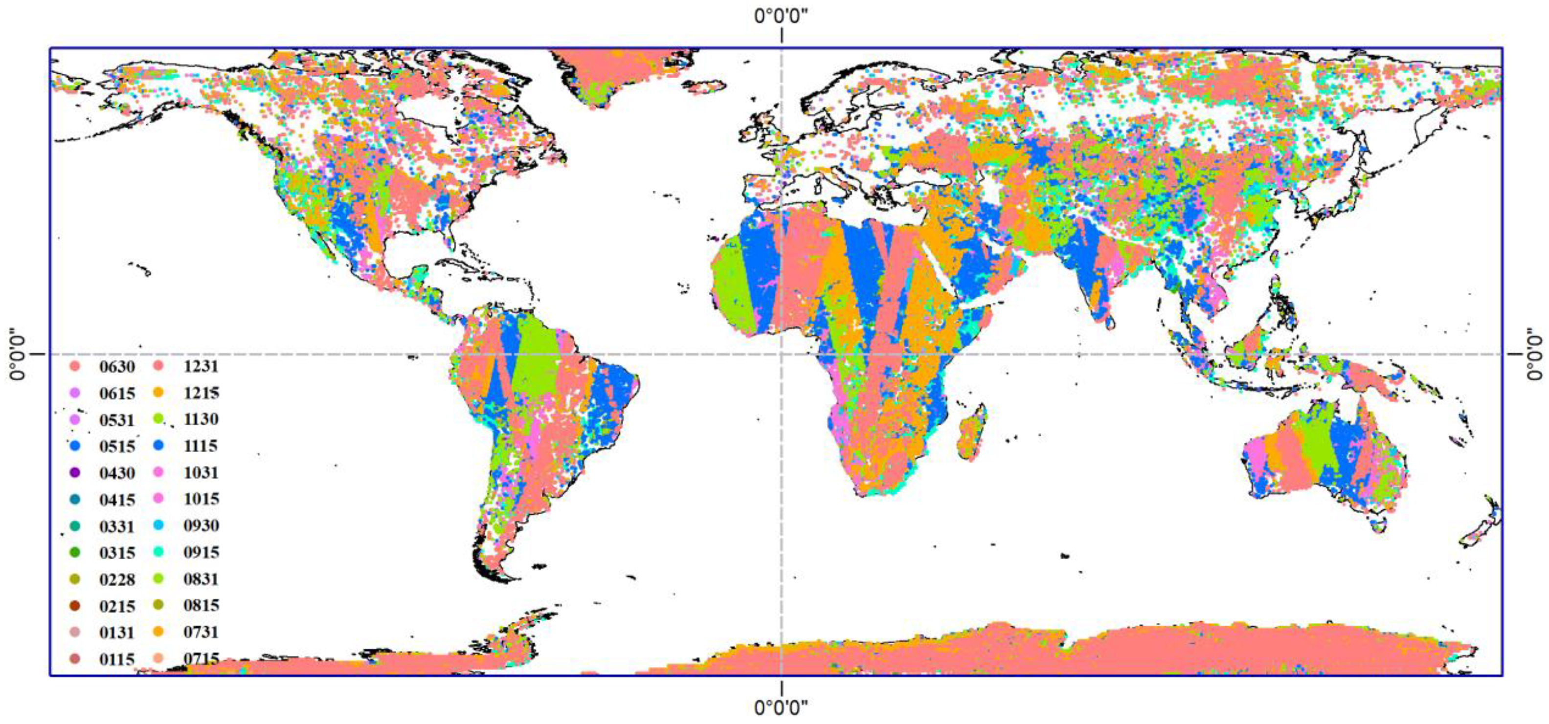
Figure 1. Spatial collocation location for FY-3D/MWRI and GCOM-W1/AMSR2 based on spatial, temporal, and geometry collocation criteria, as well as filtering with globally homogeneous pixels for the period of January–December 2022, on the 15th day and at the end of the month, for a total of 24 days (different days are shown in different colors).
Remotesensing 16 00424 g001
Figure 2. Differences in annual mean brightness temperature between FY−3D/MWRI and GCOM−W1/AMSR2 over the global land area: (a) 10.65 GHz (H; horizontal), (b) 10.65 GHz (V; vertical), (c) 18.7 GHz (H), (d) 18.7 GHz (V), (e) 23.8 GHz (H), (f) 23.8 GHz (V), (g) 36.5 GHz (H), (h) 36.5 GHz (V), (i) 89 GHz (H), and (j) 89 GHz (V).
Remotesensing 16 00424 g002aRemotesensing 16 00424 g002bRemotesensing 16 00424 g002cRemotesensing 16 00424 g002dRemotesensing 16 00424 g002e
Figure 3. Comparison of TB in each channel of AMSR2 and MWRI. The different colors indicate the aggregation of data points. The subfigures represent the following frequency and polarization combinations: (a) 10.65 GHz (H; horizontal), (b) 10.65 GHz (V; vertical), (c) 18.7 GHz (H), (d) 18.7 GHz (V), (e) 23.8 GHz (H), (f) 23.8 GHz (V), (g) 36.5 GHz (H), (h) 36.5 GHz (V), (i) 89 GHz (H), and (j) 89 GHz (V).
Remotesensing 16 00424 g003aRemotesensing 16 00424 g003b
Figure 4. The TB frequency statistics for each channel of AMSR2 (blue line) and MWRI (red line): (aj) present the frequency statistical results for the ten channels of FY−3D/MWRI and GCOM−W1/AMSR2 from 10.65–89 GHz. The Min (maximum), Min (minimum), Mean (mean), and Std (standard deviation) of TB for two sensors are shown on the left-hand side.
Remotesensing 16 00424 g004aRemotesensing 16 00424 g004b
Figure 5. The total number of matching pixels, correlation coefficients (R2), the root mean square error (RMSE), and bias values for each channel in different TB segments. All the TB values are divided into 12 segments with a TB interval of 20 K.
Remotesensing 16 00424 g005aRemotesensing 16 00424 g005bRemotesensing 16 00424 g005c
Figure 6. Land cover map with homogeneous pixels on a 25 km EASE-GRID projection grid.
Remotesensing 16 00424 g006
Figure 7. Distribution of TB differences (TBMWRI − TBAMSR2) and RMSEs between AMSR2 and MWRI data for horizontal and vertical polarizations across each channel for different land cover types. The vertical bars in the left box plot represent the upper to lower quartiles of the data, with the narrowing in the middle indicating the median value. The ends of the vertical dotted lines represent the maximum and minimum values. Points outside the vertical dotted line represent outliers.
Remotesensing 16 00424 g007aRemotesensing 16 00424 g007bRemotesensing 16 00424 g007c
Figure 8. RMSE and bias distributions of pre−calibration MWRI data and after−calibration MWRI data with respect to AMSR2 data for each channel at different TB intervals. All the TB values are also divided into 12 segments with a TB interval of 20 K.
Remotesensing 16 00424 g008aRemotesensing 16 00424 g008b
Table 1. Comparison of the FY-3D/MWRI and GCOM-W1/AMSR2 sensors.
Instrument Configurations
Satellite platformFY-3DGCOM-W1
OrbitSun-synchronous orbitSun-synchronous orbit
SensorMWRIAMSR2
Data release date1 January 201925 January 2013
Incidence angle53 degrees55 degrees
Altitude836 km700 km
Equator crossing Time
(local time zone)
2:00 p.m. ascending
2:00 a.m. descending
1:30 p.m. ascending
1:30 a.m. descending
Regression cycle5.5 days2 days
PolarizationVertical and horizontalVertical and horizontal
ScanConical scanConical scan
Dynamic range3–340 K2.7–340 K
Swath width1400 km1450 km
Channel Set
Center frequencyMWRI/FY-3DAMSR2/GCOM-W1
Band widthPolarizationGround resolutionBand widthPolarizationGround resolution
GHzMHzV.HkmMHzV.Hkm
6.925/7.3 350V.H35 × 62
10.65180V.H51 × 85100V.H24 × 42
18.7200V.H30 × 50200V.H14 × 22
23.8400V.H27 × 45400V.H15 × 26
36.5900V.H18 × 301000V.H7 × 12
892 × 2300
(double sideband)
V.H9 × 153000V.H3 × 5
Table 2. Temporal and spatial information of the auxiliary data used in this study.
AbbreviationUnitsSpatial ResolutionTemporal ResolutionSource
Land coverm500 yearlyNASA
LongitudedegSiteStatic -CMDC
LatitudedegSiteStatic -CMDC
TimehSite1 hCMDC
Cloud detectionm400015 minFY-4A
Table 3. The maximum, minimum, mean, and standard deviation (STD) values of each channel’s brightness temperature (TB). The ∆min, ∆max, ∆std, and ∆mean values refer to the differences in minimum, maximum, mean, and STD values between the two sensors.
FY-3D/MWRI (K)GCOM-W/AMSR2 (K)(MWRI—AMSR2) (K)
MinMaxStdMeanMinMaxStdMean∆Min∆Max∆Std∆Mean
10.65 H9929042.42225.109828742.64226.0013−0.22−0.90
10.65 V14930731.56254.1514730931.98255.652−2−0.42−1.49
18.7 H11129147.72226.3911129147.44226.24000.270.15
18.7 V15030832.29256.3115030832.13257.00000.16−0.70
23.8 H11129248.43230.5111329148.77231.41−21−0.33−0.89
23.8 V14630335.94250.6114530636.46251.981−3−0.52−1.37
36.5 H11529045.57223.7811428945.97224.7511−0.40−0.97
36.5 V14830135.77247.1214730436.26248.391−3−0.48−1.27
89 H13729139.62246.7913729239.66247.020−1−0.05−0.24
89 V15429730.98257.9715629930.98258.19−2−20.00−0.22
Table 4. Estimated linear correction coefficients employed for inter-calibrating FY-3D/MWRI observations at frequencies of 10.65 GHz, 18.7 GHz, 23.8 GHz, 36.5 GHz, and 89 GHz. Both vertical and horizontal polarizations are considered. These coefficients aim to align FY-3D/MWRI observations across the study area.
ChannelSlopeIntercept (K)ChannelSlopeIntercept (K)
10.65 H1.004−0.08910.65 V1.012−1.572
18.7 H0.9941.29718.7 V0.9942.287
23.8 H1.006−0.54923.8 V1.014−2.038
36.5 H1.008−0.78836.5 V1.012−1.806
89 H1.0000.24189 V0.9980.700
Table 5. Regression analysis for each channel determines the equations used for adjusting the TB of FY-3D/MWRI. The R2, RMSE, and mean bias of the calibrated MWRI data with the AMSR2 data are also listed in this table.
ChannelEquationR2RMSE (K)Bias (K)
10.65 HMWRI = 1.004 × AMSR2 − 0.0890.9981.7710.000
10.65 VMWRI = 1.012 × AMSR2 − 1.5720.9981.5760.000
18.7 HMWRI = 0.994 × AMSR2 + 1.2970.9991.7950.000
18.7 VMWRI = 0.994 × AMSR2 + 2.2870.9971.6660.000
23.8 HMWRI = 1.006 × AMSR2 − 0.5490.9991.7170.000
23.8 VMWRI = 1.014 × AMSR2 − 2.0380.9981.6090.000
36.5 HMWRI = 1.008 × AMSR2 − 0.7880.9981.8450.000
36.5 VMWRI = 1.012 × AMSR2 − 1.8060.9981.7020.000
89 HMWRI = 1.000 × AMSR2 + 0.2410.9981.9260.000
89 VMWRI = 0.998 × AMSR2 + 0.7000.9961.9190.000
Disclaimer/Publisher’s Note: The statements, opinions and data contained in all publications are solely those of the individual author(s) and contributor(s) and not of MDPI and/or the editor(s). MDPI and/or the editor(s) disclaim responsibility for any injury to people or property resulting from any ideas, methods, instructions or products referred to in the content.