Nested Cross-Validation for HBV Conceptual Rainfall–Runoff Model Spatial Stability Analysis in a Semi-Arid Context

Abstract

Accurate and efficient streamflow simulations are necessary for sustainable water management and conservation in arid and semi-arid contexts. Conceptual hydrological models often underperform in these catchments due to the high climatic variability and data scarcity, leading to unstable parameters and biased results. This study evaluates the stability of the HBV model across seven sub-catchments of the Oum Er Rabia river basin (OERB), focusing on the HBV model regionalization process and the effectiveness of Earth Observation data in enhancing predictive capability. Therefore, we developed a nested cross-validation framework for spatiotemporal stability assessment, using optimal parameters from a donor-single-site calibration (DSSC) to inform target-multi-site calibration (TMSC). The results show that the HBV model remains spatially transferable from one basin to another with moderate to high performances (KGE (0.1~0.9 NSE (0.5~0.8)). Furthermore, calibration using KGE improves model stability over NSE. Some parameter sets exhibit spatial instability, but inter-annual parameter behavior remains stable, indicating potential climate change impacts. Model performance declines over time (18–124%) with increasing dryness. As a conclusion, this study presents a framework for analyzing parameter stability in hydrological models and highlights the need for more research on spatial and temporal factors affecting hydrological response variability.

1. Introduction

Each year, multiple countries face a rising water crisis, linked to limitations in water availability, that will endure for at least the upcoming few decades [1,2]. Several combined factors, including global warming aggravation, the disturbance of natural water regimes, population growth, and the increasing global demand for water, cause the contemporary water scarcity situation [3,4,5,6]. As a result, the alternation of natural and induced positive feedback has the potential to significantly affect the whole water cycle of individual or large river basins, consequently decreasing freshwater availability [7,8].

Thus, the water crisis indicators manifest as an increase in demand and a decrease in supply. Global water consumption has increased by approximately 1% per year over the last few decades, with the agricultural sector representing most of it, accounting for about 80% of total use. Per contra, worldwide terrestrial water storage capacity has marked a decline of about 5% to 20% by 2050, especially in the Southern Hemisphere [7,9,10,11,12]. Hence, this scenario has significantly influenced the water supply, making the management of available water quantities, despite its scarcity, a more complicated mission and engendering additional challenges for water sector managers on several levels.

On a smaller scale, these issues become more severe, i.e., in the southern side of the Mediterranean basin, North Africa, and Morocco, where the situation is not much better. They are regions with mostly arid and semi-arid climates, where the scarcity of rainfall and high evaporation rates are the dominant characteristics [13]. In this regard, numerous studies conducted in the Mediterranean basin and Morocco scale concluded that climate change has actual effects on the water regimes and hydrological cycle upstream, as well as downstream [14,15,16,17,18,19,20], including, for example, changes in surface runoff quantities and evaporation rates [21] and the elongation of the dry season at the expense of the wet season. There is an abnormal variation in surface runoff rates between the dry and humid seasons. This variation is characterized by sharp increases in precipitation intensity, leading to higher surface runoff rates during the dry season. Conversely, the humid period has become shorter, with reduced surface runoff rates. This period also shows considerable spatial variation in runoff rates. These changes have led to a general decline in water storage and production rates in the respective basins [22,23].

In this context, and to effectively manage the available water resources, scientists and researchers in the field of hydrology have been forced to develop practical management strategies and tools for this valuable resource. Most often, these tools take the form of simplified, logical models and equations to simulate natural processes (specifically the hydrological cycle) [24].

In practice, hydrological models describe the spatial average of the relationships and interactions between all the processes that compose the water cycle as a group of linked variables and reservoirs. Regarding conceptual models, each reservoir acts according to the process that occurs within it to estimate, with a certain degree of bias and uncertainty, the amount of rain, snow, and hail that becomes runoff in a watershed [25,26,27,28].

For this purpose, the development of hydrological modeling, like that of other scientific research fields, has gone through several major historical stages since the 1960s, influenced mainly by the purpose of the model, the availability and type of input data, the material of processing, and the modeler responsible for conceptualizing and building the model [29,30]. In this regard, each stage of development has produced a distinct type of rainfall–runoff model. Accordingly, each model improves on the previous one, mainly in accuracy and spatiotemporal resolution.

Indeed, several studies have demonstrated that hydrological models, in general, and particularly conceptual models such as the HBV model, are capable of reproducing the streamflow in the studied watersheds under contrasted climate conditions and with as few parameters as possible [31]. During the calibration and validation periods, the simulation performances range from moderate to excellent [32,33,34,35,36,37].

The model estimates streamflow at a daily temporal resolution and requires little input data and computing time, so it has gained the name parsimonious. The latter is one of its advantages, in addition to its high performance and persistence compared to other overparameterized models [38]. The model has shown high streamflow predicting efficiency in many studies dealing with hydrological modeling in ungauged or poorly gauged basins of different sizes and hydroclimatic contexts, the evaluation of the effects of climate change on the water balance, floods assessment, or those concerned with studies related to hydraulic energy [39,40,41,42].

However, there is still a notable gap, at least in a regional context, regarding the problem of instability or stability in the structure of hydrological models. Specifically, by stability, we mean the ability of the structure, parameters, or accuracy of model outputs to withstand transfer from one basin to another or exposure to changing hydroclimatic conditions over time. Few studies have explored model stability in terms of accuracy across varying spatiotemporal and hydrological conditions [43,44]. Relative amounts of bias in hydrological models strongly depend on time and space scales and their changes [45,46,47]. Thus, hydrological model stability holds great theoretical and practical importance to improve performance and make these models more reliable for water management issues.

Many researchers have conducted studies on the stability of hydrological model parameters and performances using regionalization to transmit catchment information, either directly by using improved and calibrated parameters in a well-gauged basin (donor) and then applying them to the rest of the poorly gauged basins (target), considering explicitly climatic and/or physiographic similarity [48,49,50,51,52,53,54], or indirectly by calibrating and validating the structure of one model and applying the same model structure to other basins with different hydroclimatic characteristics [55]. According to Seibert [55], most of the results indicate that transferring a well-calibrated model from a donor basin to a target basin can yield reasonably accurate results, though not necessarily identical to those achieved by a model calibrated specifically for the target basin. Besides, strategies based on transferring calibrated model parameters from one basin to another, using a specific measure of climatic and/or physiographic similarity, outperform other methods, including the indirect method mentioned previously [56,57,58,59,60,61,62].

The issue of identifying and understanding the potential mechanisms and features that control the parameterization of the hydrological model in terms of changes in hydroclimatic conditions of watersheds is still far from being resolved [63]. Hence, the importance and originality of this study aimed to investigate the stability of the HBV model and its parameters when transferred from one watershed to another.

In this research, we used the same structure of the calibrated and validated HBV model following the strategy used by [35] in a donor basin, as well as the optimal parameters set produced in the calibration and validation stages, to carry out nested cross-calibration and cross-validation (NCV) in the target basins interchangeably.

To implement the developed approach for various applications we seek, we designed and performed NCV. This was for a spatiotemporal stability assessment framework of the HBV model, using an 18-year (2001–2019) + 1 year of warm-up (2000–2001) time series of in situ hydroclimatic data from (P, Q, T) the Oum Er Rabia river basin (OERB) gauging stations’ remotely sensed/reanalysis data (CHIRPS, MODIS SCA, ERA5) over seven sub-catchments of the OERB river basin. We obtained a complete set of the optimal parameters using a pre-calibrated model from a donor catchment for running the same model structure over the target catchments both spatially and temporally, tuning the model parameters and interchangeably studying the roughness of surface parameters of the model and their effect on the performance of the model, as well as its ability to reproduce the flow with the same accuracy or not, using the well-known objective functions used in hydrological studies for calibration performance assessment, namely Kling–Gupta efficiency (KGE), Nash–Satcliffe efficiency (NSE), coefficient of determination (R²), root mean square error (RMSE), and relative volume error (RVE), to ensure that the accuracy measures obtained truly characterize the variability in hydroclimatic conditions from one basin to another and how a single model structure behaves when generalized to other catchments and periods in a semi-arid context.

Overall, this work aims to answer the main following questions:

−

Can the calibrated HBV model maintain accuracy in reproducing streamflow across various sub-catchments with differing hydroclimatic conditions?

−

How stable are the HBV model parameters when transferred between different sub-catchments within the OERB river basin?

−

What is the impact of spatiotemporal variability on the performance of the HBV model in a semi-arid context?

2. Materials and Methods

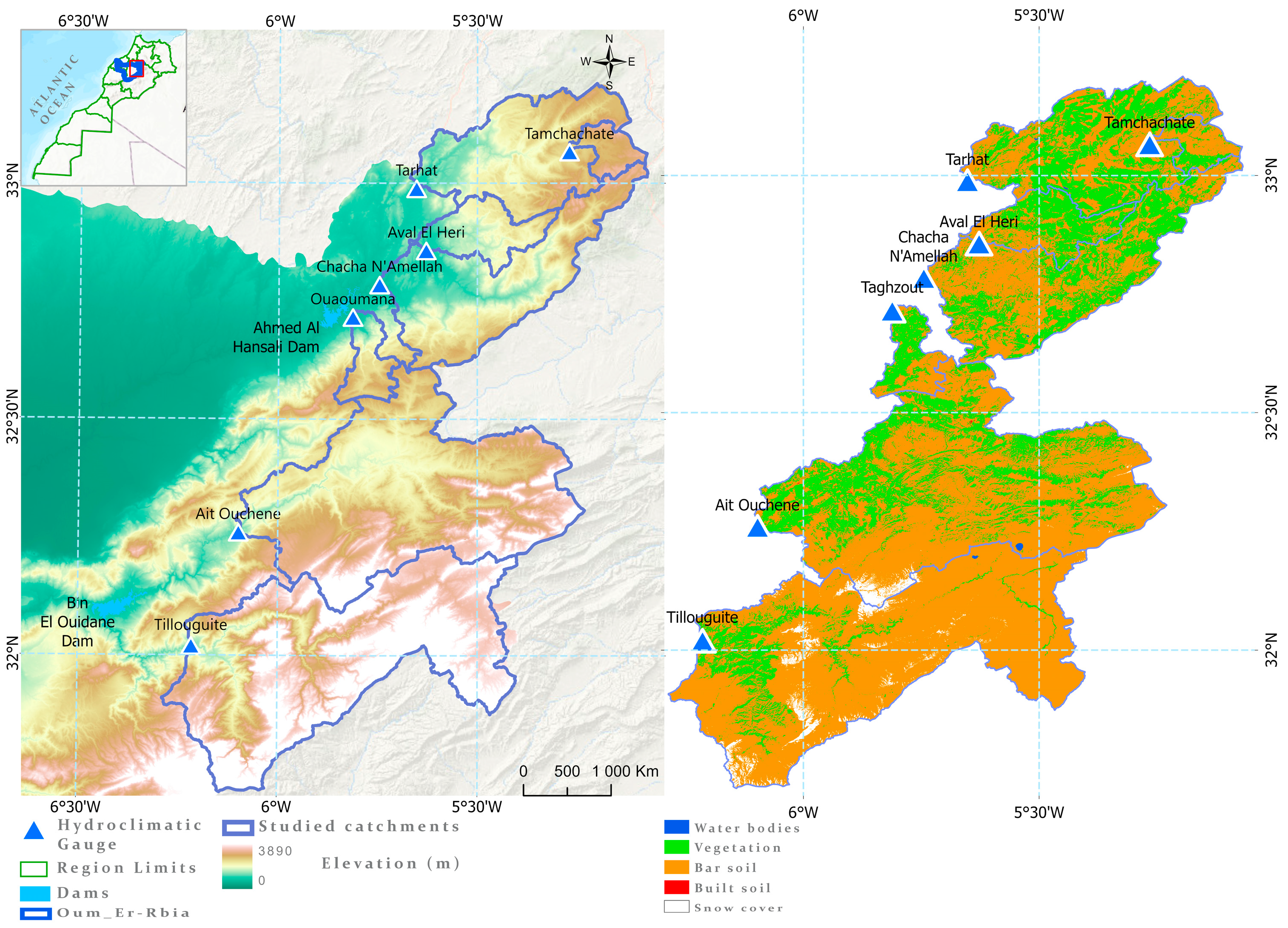
2.1. Study Catchments

The OERB basin is located in the center of the Moroccan Kingdom (Figure 1), with about 38,000 km² of drainage area. The basin, particularly the upper part, is of critical importance due to its abundance of freshwater, both in terms of surface fluxes and groundwater recharge. This quantity of water plays a vital role in supporting various sectors such as domestic use, agriculture, mining (especially phosphate), and hydropower generation. Hydrological processes in the basin are complex, deriving water from direct precipitation, infiltration, and snowmelt from the peaks of the Atlas Mountains [64,65]. However, the OERB basin faces many challenges and constraints. The impacts of climate change, as examined by [66], and increased drought frequency, as reported by Strohmeier et al. [65], represent serious challenges to water supply. Ouatiki et al. [67] demonstrated the tendencies of hydrological change throughout the basin. These difficulties necessitate sustainable water management strategies to assure the long-term availability of water supplies for all affected sectors. We focus in this study on the mountainous sub-basins for considerations mainly related to the hydroclimatic data availability, at least for streamflow data, and to make the modeling more representative and realistic, we consider the sub-site concerned by the study to be a total of seven sub-catchments of the Eastern part of OERB upstream

Table 1. Summary acronyms and physiographic and hydrologic features of seven studied catchments.

Basin		Catchment Characteristics				Hydrologic Characteristics
ID	Name	Area (Km2)	Slope (%)	P (mm/Day)	Q (m3.s−1/Day)	AET (mm/Day)	SWE (mm/Day)	MSI	VF
AOCH	Ait Ouchene	2381	26.3	1.24	9.90	4.08	0.81	1.04	0.65
AVHE	Aval El Heri	329	17.8	1.67	2.39	4.02	0.12	0.92	0.77
CHNA	Chacha N’Amellah	1400	19.6	1.50	8.67	3.98	0.14	0.98	0.78
TAGH	Taghzout	208	21.1	1.49	0.92	4.01	0.13	1.04	0.72
TAMC	Tamchachate	340	13.8	1.90	0.79	3.83	0.38	1.04	0.70
TARH	Tarhat	1026	18.1	1.71	12.11	3.93	0.21	1.00	0.78
TILL	Tillouguite	2030	33.9	1.16	14.39	4.09	0.65	1.15	0.71

Note. The statistics are daily averaged throughout 2001–2019 of rainfall (P), streamflow (Q), actual evapotranspiration (AET), snow water equivalent (SWE) from GLDAS-2.1, vegetation fraction (VF) from MODIS, and moisture stress index (MSI) from SMAP.

.

The annual average precipitation in the OERB is about 550 mm annually, with contrasted differences between the upstream and downstream levels, reaching 800 mm in the high (Middle Atlas) and 300 mm in the low [68]. In low compared to high altitudes, the annual mean temperature is 18 °C (with highs of over 40 °C in August and lows of 0 °C to 4 °C in January). Recently, the temperature has reached extreme values that may attend −9 °C as an absolute minimum in winter and 47 °C as the absolute maximum in the summer period. This in turn affects evaporation and evapotranspiration rates, increasing directly with temperature. Snow cover area (SCA) changes drastically from season to season. Most snow falls during the winter months (December, January, and February), when 36 to 60% of the basin is covered [22,69,70,71].

2.2. Data Collection and Model Description

2.2.1. Data Collection

To reproduce streamflow in each sub-basin, and given the scarcity of data in the study area, we used an integrated hydroclimatic database of 18 years (2001–2019) that combines in situ time series of daily precipitation measurements (91% ground measurements) and streamflow values (100% from gauging stations), measured on the ground taken from ABHOER gauging stations located at the outlet of each sub-basin. In case of missing data, we use ERA5-Land reanalysis data and temperature generated by interpolation using the lapse rate method from [72] and CHIRPS V2.0 data for precipitation and snow cover area (SCA) derived from the MODIS SCA satellite product MOD10A1 V6 with 500 m of spatial resolution to fill the missing values. Filled data make up a significant part of the dataset. Snow cover area (SCA), temperature (T), and potential evapotranspiration (ETP) data were fully obtained from Earth Observation (EO). In summary, 70% of the input data comes from EO and 30% from measuring stations.

We have chosen those products because of their high effectiveness in simulating river flows in semi-arid regions [70,73,74,75]. Finally, for data validation, we estimated the distribution of daily and monthly potential evapotranspiration (ETP) based on the measured time series of temperature values using the Thornthwaite formula [76].

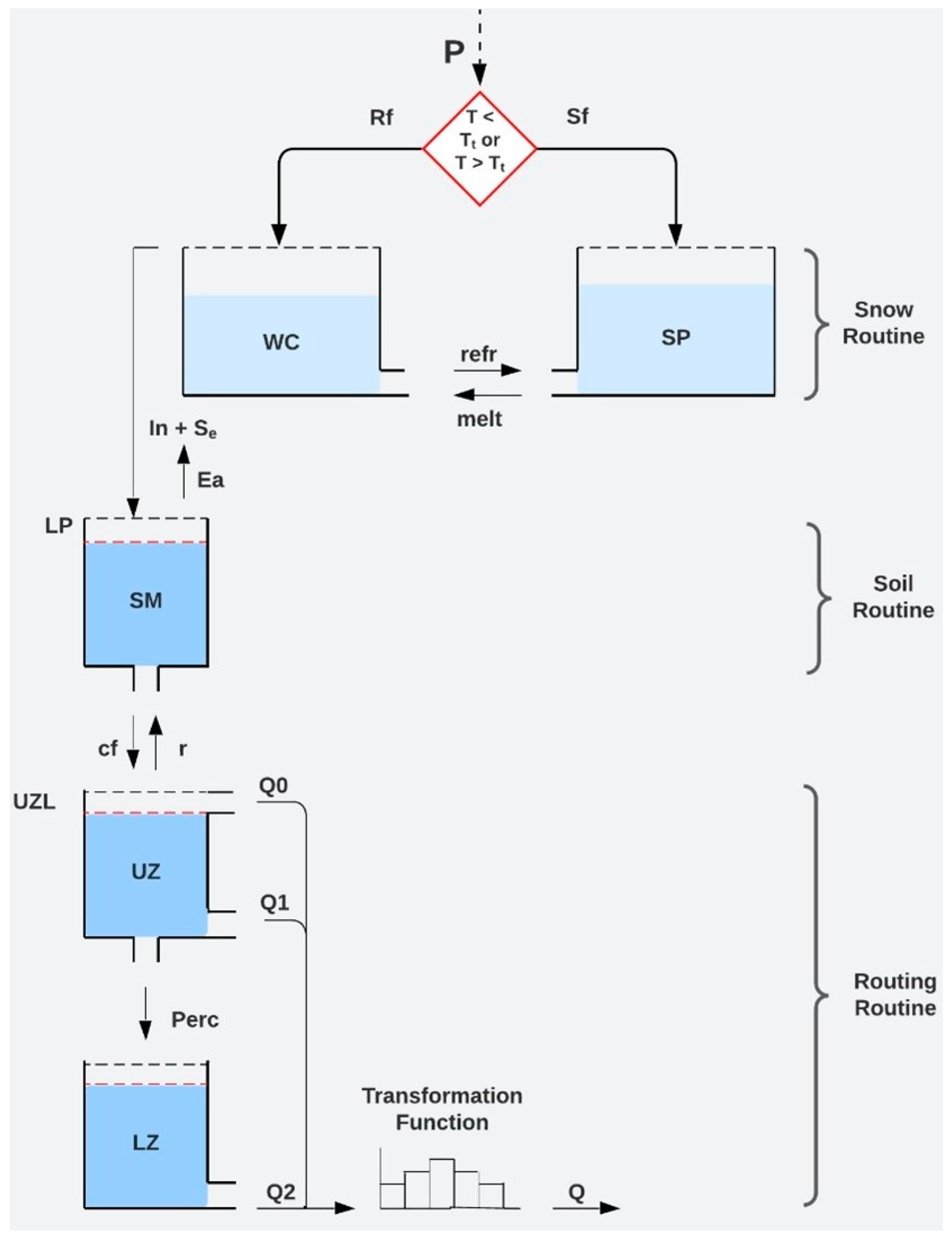
2.2.2. Model Description

To keep the modeling process as simple and efficient as possible, we used the Hydrologiska Byråns Vattenbalansavdelning (HBV) model [77,78,79] in its MATLAB 2021a user-friendly modeling Toolbox script version developed by Aghakouchak and Habib (2010) [25] and mounted by Ouatiki et al. [35]. HBV is a conceptual model with basic, simple routines that contain just a small number of parameters (Table 1).

The structure of the HBV model has always been a subject of testing its stability, adaptation, and suitability to the relevant study areas, especially when transferred from one basin to another [55,56,80,81,82]. The HBV model consists of four interconnected routines (Figure 2). Each routine describes a different component of the water cycle. Those components are snow accumulation and melting, soil moisture and subsurface dynamics, and routing. Note that the adopted version of the model does not contain a detailed description of the snow routine; it simply follows the standard algorithm implemented in the HBV model. However, it does not neglect the amount of water resulting from snow melting but incorporates it whenever there is a snow event by setting a snow melt threshold (TT: if the temperature is above) and converting it according to a degree-day factor (DDF). Additionally, the soil routine simulates soil moisture patterns in the upper part of the soil. In this regard, we can distinguish several parameters. Firstly, field capacity (FC), or the upper limit of soil moisture content, means the maximum soil moisture holding capacity (mm). The second parameter is the evaporation threshold (LP), which indicates the upper limit of (potential) evapotranspiration occurring. Thirdly, the BETA (BETA) parameter means the shape coefficient. It defines the distribution and dynamics of water through the soil layers. Finally, (ETF) is the potential evapotranspiration correction factor. The flow of effective rain (Q0) and excessive soil moisture are redirected to the upper reservoir, which shares, according to a percolation coefficient (KPERC), a portion of underground water flow to the lower reservoir. The exceedance of the two reservoirs at each time is translated by two subsurface flow (Q1) and baseflow (Q2), according to (K0), (K1), and (K2) recession coefficients.

2.3. Calibration and Validation of the Model

Initially, we performed the HBV model calibration and validation using an 18-year time series of input variables in the donor catchment (AOCH). We used the hydrological year (2000–2001) to warm up the model to obtain the initial state variables. The parameter set combinations are generated randomly using parameter ranges in

Table 2. List of the hydrological model parameters and ranges used in the model’s calibration.

Model Parameter	Routine	Unit	Range (Min–Max)
Shape coefficient (BETA)	Soil	-	1–4
Temperature correction factor (C)	Snow	°C−1	0.01–0.3
Degree day factor (DDF)	Snow	mm °C−1 d−1	0.1–0.6
Field capacity (FC)	Soil	mm	200–600
Very fast storage coefficient (k0)	Runoff	d−1	0.1–0.6
Fast storage coefficient (k1)	Runoff	d−1	0.01–0.2
Slow storage coefficient (k2)	Runoff	d−1	0.01–0.15
Percolation rate (Kp)	Runoff	d−1	0.01–0.3
Upper storage coefficient (UZL)	Runoff	mm	5–25
Limit for potential evapotranspiration (LP)	Soil	-	0.3–1

. Then, the simulation was done for the rest of the years (2001/2002 to 2018/2019), using an 18-fold cross-validation technique by time-splitting input data series and allocating a 1-year moving window for calibration and the remaining years for validation [84].

The simulation performance calibration and validation strategy has used Monte Carlo simulations and a combination of objective functions for calibration and performance assessment (e.g., Nash–Sutcliffe efficiency (NSE), Kling–Gupta efficiency (KGE), root mean square error (RMSE), Pearson correlation coefficient (R²), and relative volume error (RVE)). Specifically, we used NSE and KGE as calibration functions in a simple sequential calibration and validation approach, which involves first calibrating the model using the NSE metric. After obtaining a good NSE result, we refined the calibration using KGE to ensure that other aspects like bias and variability were well represented, while RMSE, R², and RVE were used for bias assessment. Finally, we selected the top 5% of the best-performing parameter sets based on KGE and NSE as the optimum set.

With these conditions and arrangements, the model ran over 10,000 × (7 sub-catchments × 18 years) Iteration times, totaling about 1.8 million iterations, and each time, the model’s predictive capabilities and the corresponding combination of optimal parameter values were simultaneously measured and stored. In addition to the variables related to the reservoirs, we measured the water flows and state variables.

Primarily, we will focus on the measures of the model’s predictive performances and the combination of optimal parameter values corresponding to them. We build on previous research to define the 5% of the top KGE and NSE values and their corresponding combinations of parameters as behavioral sets or runs for the 18 years of simulation [85]. According to [86], we consider these periods of high “parameter identifiability” because they include a large quantity of information for identifying a specific parameter set. These parameters will later serve as narrower forcing parameter ranges, defined by the minimum and maximum values of the resulting parameter set, for regionalization in the target basins.

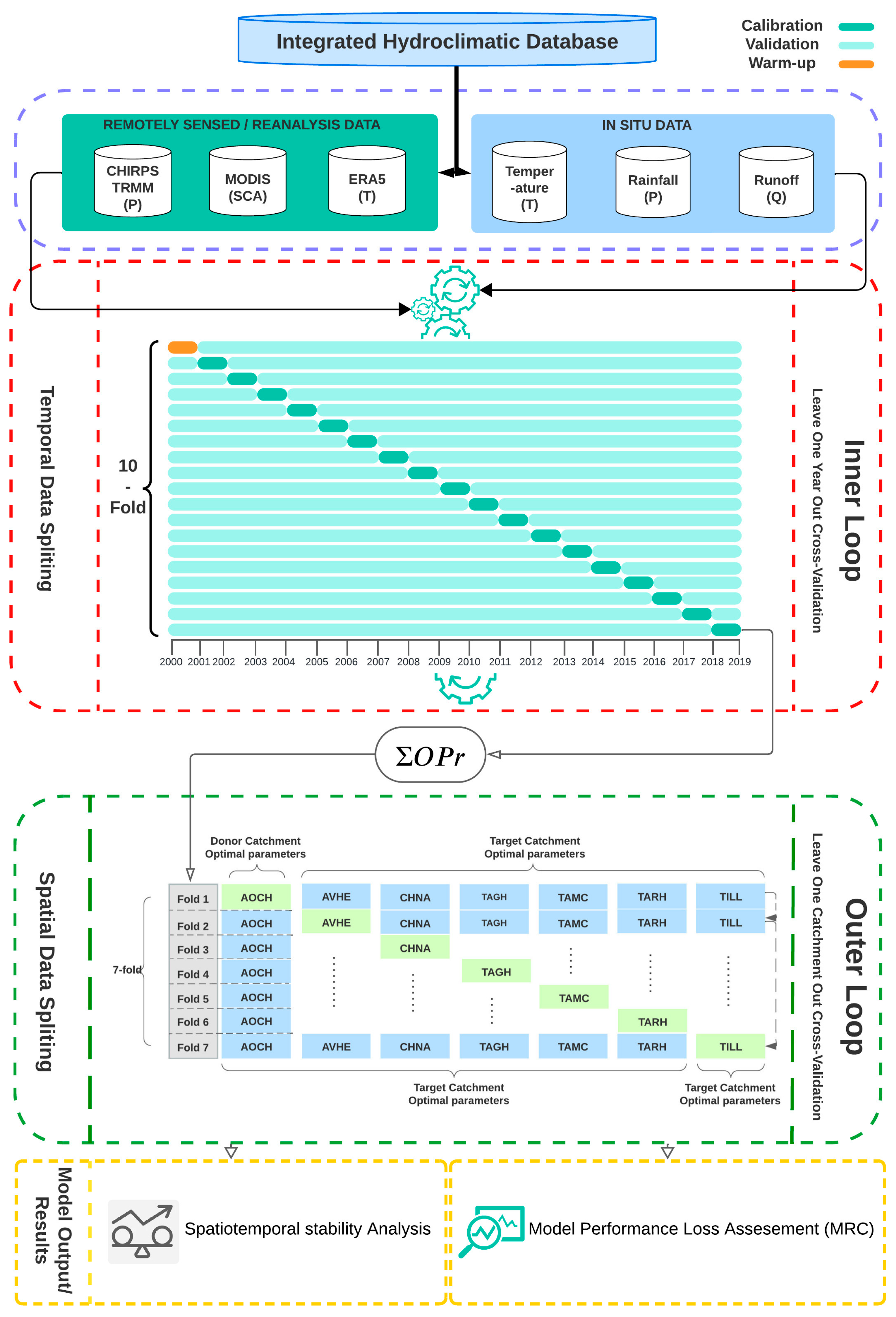
2.4. Nested Cross-Validation

To investigate the spatiotemporal stability of the HBV model in the case of regionalization of parameters to poorly gauged basins, we used a systematic approach that includes four basic steps as showed in Figure 3:

• Gathering hydroclimatic, remotely sensed, and GIS databases from multiple sources relevant to the studied sub-catchments.
• Cross-calibration and validation of the HBV model structure in a donor catchment (AOCH).
• Regionalization of model optimal parameters obtained in the donor catchment (AOCH) to target catchments using nested cross-calibration and validation over 18-year dataset and over 7 sub-catchments of the study area, according to two nested loops:
  • Inner Loop: Leave-one-year-out cross-validation for the regionalization of optimal parameter sets obtained from hydrological modeling in the donor catchment from year to year.
  • Outer Loop: Leave-one-catchment-out cross-validation for the regionalization of the HBV conceptual model from basin to basin.
• Analyzing the model performances and selecting stable optimal parameters for all the sub-catchments.

2.4.1. Temporal Cross-Validation of the Model: Leave One Year Out

Inner loop: Considering a 1-year calibration timestep, we pass a one-year calibration time window (leave-one-year-out method) [87] over the remaining simulation duration to repeatedly cross-validate and select the most efficient and stable optimal parameter set of the HBV model in each of the seven donor basins. There are 18 blocks in this loop. This number is equal to the length of input data.

2.4.2. Spatial Cross-Validation of the Model: Leave One Catchment Out

Outer loop: In the cross-validation process, we recalibrate and validate the HBV model using the optimal parameters from the donor basin. This helps us to narrow the parameter ranges for Monte Carlo simulations in the target basin [24]. Each time, the optimal parameters for the 5% of the operating running cycles of the most efficient model runs are acquired and used for calibration in the next catchment, regardless of its area, physiological characteristics, or quality of its input data. The spatially moving window is the hydrological unit (sub-catchment) resulting from the catchment delineation based on considering each measuring station as a surface runoff outlet (7 blocks of cross-validation = the number of sub-catchments studied). In each cycle of the outer loop, alternately, we leave one donor catchment out for calibration and the rest of the catchments designated as target catchments for validation [88,89,90].

2.4.3. Performance Metrics

To compare simulated and observed streamflow, hydrological model performance criteria are often used during calibration and evaluation, generating a single numerical value that indicates the degree of agreement [91]. Traditionally, the Nash–Sutcliffe efficiency (NSE) is a commonly used objective measure in hydrological studies, favored for its efficiency in evaluating the performance of various simulation models and its standardized interpretation of model performance [92,93].

$$NSE=1-{{\displaystyle \frac{{\sum }_{t=1}^{t=T}(Q_{sim}\left(t\right)-Q_{obs}\left(t\right))}{{{\sum }_{t=1}^{t=T}(Q_{obs}\left(t\right)-\overline{Q_{obs}})}^2}}}^2,$$

(1)

In addition, root mean square error (RMSE) is employed to offer a comprehensive overview of the error distribution. RMSE is expressed in units of m³/s.

$$RMSE=\sqrt{{{\displaystyle \frac{{\sum }_{i=1}^n(Q_i^{obs}-Q_i^{sim})}{n}}}^2},$$

(2)

Kling–Gupta efficiency (KGE), introduced by Gupta et al. [94], addresses some limitations of NSE and is increasingly adopted for model calibration and evaluation. The inclusion of KGE in the evaluation toolkit is motivated by the inherent variability in hydrological features within arid and semi-arid contexts. KGE is often considered superior to NSE because it decomposes model performance into three distinct components: correlation, bias, and variance, whereas NSE focuses primarily on the correlation between observed and simulated data. Thus, KGE provides a more balanced assessment of model performance, especially in cases where hydrological models may exhibit reasonable correlation but struggle with bias and variance, which are critical for assessing water balance and flow dynamics, especially in arid and poorly or irregularly measured climates. Therefore, there is a growing need for a tool that can assess hydrological behavior from different perspectives. NSE may not capture these nuances effectively, especially in regions where flows are intermittent or highly variable, which is common in arid and semi-arid regions. This is particularly important in our study area, where we aim to ensure that the model accurately captures the flow variability and not just the overall pattern. This broader perspective provided by KGE ensures a more robust assessment of model performance, which is critical in such data-limited environments. This emerging metric complements existing criteria and contributes to a more comprehensive assessment of model performance.

$$KGE=1-\sqrt{{\left(r-1\right)}^2+{\left(\alpha -1\right)}^2+{(\beta -1)}^2},$$

(3)

where:

• r: The Pearson correlation coefficient between the simulated and observed data;
• α: The ratio of the standard deviation of the simulated values to the standard deviation of the observed values.
• β: The ratio of the mean of the simulated values to the mean of the observed values.

This study goes beyond traditional metrics, incorporating KGE alongside NSE, RMSE, R², and RVE and emphasizing the importance of maximizing KGE, NSE, and R² metrics against RMSE and RVE-defined metrics for a holistic evaluation of hydrological models.

Besides, R² is a goodness-of-fit measure that indicates how effectively the independent variable(s) explain the variability of the dependent variable in a regression model. It is the squared correlation between the model’s observed and predicted values. It runs from 0 to 1, with 1 signifying a relatively good match between the model and the data [95].

$$R^2={\displaystyle \frac{{({\sum }_{i=1}^n(y_i-\overline{y})(y_i^1-\overline{y^{\prime }}))}^2}{{\sum }_{i=1}^n{(y_i-\overline{y})}^2{\sum }_{i=1}{({y^{\prime }}_i-\overline{y^{\prime }})}^2}},$$

(4)

$$RVE={\displaystyle \frac{{\sum }_{i=1}^n(y_i-{\overline{y}}_i)}{{\sum }_{i=1}^n{y}_i}},$$

(5)

The RVE represents the model’s total water balance, representing the variation in mean flow over time. A low RVE, like MRE and MSRE, does not always indicate accurate forecasts because positive and negative mistakes can cancel one other out. While a perfect model scores zero, one that is unconnected to the real hydrograph might also have an RVE of zero [96,97].

2.4.4. Model Performance Assessment

Coron et al. [98] established the model robustness criteria (MRC), which measures the performance losses that occur when optimized parameter sets transition across independent validation periods and locations. Equation (6) expresses this.

$${MRC}_{D\to T}={\displaystyle \frac{{\epsilon }_{D\to T}}{{\epsilon }_{T\to T}}}-1$$

(6)

where ε in the equation denotes the performance criteria optimized during calibration (in our case, KGE, NSE, and R²); we calculate the efficiency difference of the model between the donor and recipient parameters. The idea behind MRC is that an optimal parameter set obtained during the calibration period for a given time or space functions as the donor parameter set (D) for a model application on a validation target (T) period or catchment. The interpretation of MRC values is as follows: The indicator takes a zero if the modeling efficiency using the optimized set of parameters in the donor catchment (D) is the same as in the target catchment (T). A positive increasing value of MRC means that the parameter set transferred from the donor basin becomes less appropriate in the target basin, which means a higher bias and, thus, a model performance loss. On the other hand, negative values mean that the optimized parameter set in the donor basin leads to better performance results and bias decreasing in the target catchment than those optimized in the donor basin itself.

3. Results and Discussion

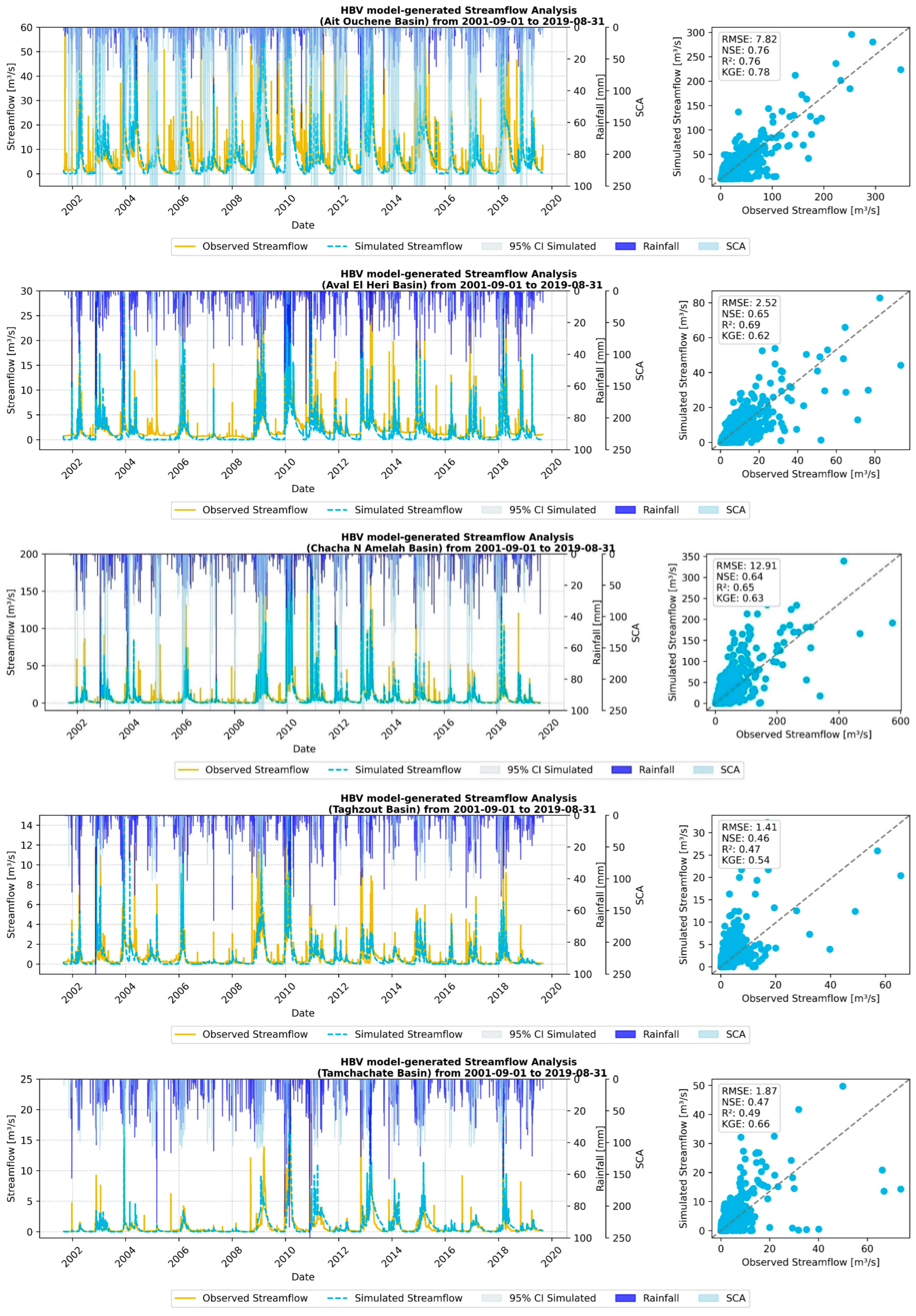
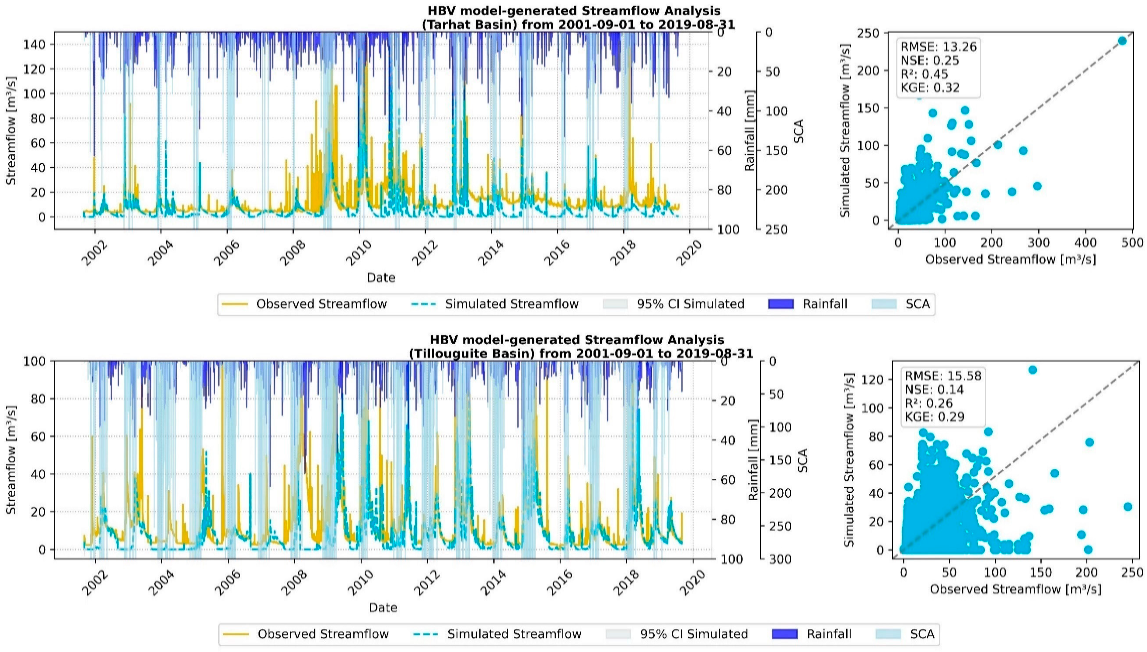
3.1. Model Simulation Performances in Donor Catchment

The results of the cross-calibration and validation of the HBV model over Ait Ouchene (AOCH) in

Table 3. Values of the combination of optimal parameter sets of the mean of 5% best of KGE and NSE values.

Catchment	BETA	C	DD	FC	K0	K1	K2	L	Kp	LP	KGE	NSE	R2	RMSE	RVE
AOCH	2.3451	0.0917	0.4694	236.8616	0.4018	0.0833	0.0262	22.0232	0.0690	0.6031	0.8087	0.8042	0.9195	16.1107	−0.2971
AVHE	1.0072	0.0101	0.4825	210.8385	0.2286	0.1021	0.0180	15.1770	0.2925	0.6888	0.7749	0.6716	0.8275	5.5344	−0.1680
CHNA	1.0086	0.0195	0.4122	221.8037	0.4684	0.1554	0.0350	10.7412	0.1780	0.4693	0.7029	0.7522	0.8722	27.1942	−0.2117
TAGH	1.2290	0.0120	0.2356	560.7553	0.5943	0.0866	0.0819	23.6163	0.0300	0.4225	0.7645	0.6166	0.7891	2.5682	−0.1786
TAMC	3.4315	0.0373	0.5252	584.0452	0.1949	0.0147	0.0770	24.9868	0.2965	0.3195	0.5385	0.5468	0.7433	5.1625	−0.2123
TARH TILL	1.0965	0.2575	0.3743	258.0857	0.1683	0.0598	0.0389	17.8828	0.2659	0.6214	0.4860	0.4006	0.6493	24.1965	−0.1091
	1.0812	0.2310	0.5698	205.0131	0.1878	0.0170	0.0705	21.1327	0.2616	0.3953	0.2308	0.2175	0.5163	24.6555	−0.2865

Note that, each parameter set combination in the table above constitutes subsequently the donor calibration parameters for each fold of seven-fold when we do the spatial data splitting.

and Figure 4 show moderate interannual variation depending on whether the year was dry or wet. The model generally simulates runoff with high performances up to 0.80 for both KGE and NSE metrics and 16.11 m³/s of mean RMSE metric that we consider high bias values if compared to KGE and NSE values. We can explain the high RMSE values by the significant amounts of precipitation received by the basin during the calibration year.

The high RMSE values can be explained by the significant amounts of precipitation received by the basin during the calibration year. Moreover, the model reliably reproduces the streamflow at the outlet in each timestep, especially during the wet period of the year characterized by high flow rates [36]. Furthermore, Figure 4 reveals that the model performs well with a maximum relative error of roughly ±0.3 of mean RVE during dry periods but with an underestimation of streamflow, and it is clear that for the TILL basin, there was a considerable amount of precipitation (Mean RMSE = 24.65 m³/s) in the period 2009/2010 but the model does not perform well (KGE = 0.23). The main reason for the underestimation of the HBV model outputs is often due to the neglect of the role of snowmelt water and the weakness of the SWE simulation routine in the model. These findings aligned with the research of Sleziak et al. [99], who concluded that not adequately weighting the snow component in water modeling frequently leads to an underestimation of modeling outputs and can reduce model accuracy and stability.

However, in the TAMC, TARH, and TILL sub-catchments, the results reveal that the HBV model fails to reproduce the flow to some extent and exhibits biases during periods of high flows, resulting in disproportionately high RMSE values when compared to other metrics with no relevance of KGE or NSE values. This discrepancy can be attributed to the model’s sensitivity to peak flows, exacerbated by low infiltration rates [79,100]. As evident from the LULC map (Figure 1), the poorest model performance (NSE = 0.14 and KGE = 0.29) corresponds spatially to the TILL catchment, which contains the largest proportion of bare soil. This decreases infiltration rates and, consequently, increases runoff volume and velocity [101]. Moreover, this sensitivity is more pronounced in the catchments with significant inter-annual variability in precipitation [35,80,102]. In addition, the model’s performance under dry conditions across years was less satisfactory, especially in simulating low flows. Uncovering this limitation is crucial, as dry-season low flows are critical for water resource management in arid and semi-arid regions.

The poor representation of low flows may also stem from several factors. Firstly, the semi-arid region where the studied sub-catchments exist experiences considerable spatial rainfall variability. Rainfall in these regions tends to be highly localized, often driven by convective storms that can result in vastly different precipitation amounts within short distances [103,104,105]. Considering the lumped structure of the HBV model that relies on spatially aggregated inputs, it cannot capture this fine-scale variability in rainfall patterns. In reality, localized rainfall events in semi-arid regions lead to patchy runoff generation, where some areas generate surface flow while others do not, depending on the storm’s location. Hence, the HBV model cannot account for this spatial heterogeneity, which leads to lower model performance during dry periods, when only small areas might receive sufficient rainfall to generate runoff [106].

Additionally, flow transmission losses are particularly important in the studied catchments and other semi-arid regions. Flow transmission losses refer to water infiltration into the riverbed as it travels downstream, reducing the water volume that reaches the catchment outlet. This latter is a common feature of ephemeral or intermittent streams, which are prevalent in semi-arid regions [107,108]. Unfortunately, the HBV model, being conceptual and designed for perennial streams, does not explicitly account for this process, leading to an overestimation of streamflow during low-flow periods [109]. As a result, while the model performs well during wet periods, it systematically underestimates water losses in dry years and consequently overestimates low flows. Future studies may need to integrate a process-based model that includes transmission losses to improve simulation accuracy in arid and semi-arid environments.

Given the model’s high efficiency during the calibration and validation phases in the AOCH donor catchment, as well as the optimal set of parameters that will serve as initial input values for the model, we can now proceed to the next stage of our integrated modeling approach.

3.2. Regionalization of Model Optimal Parameters Obtained from Donor Catchment (AOCH) to Target Catchments Using Nested Cross-Calibration and Validation

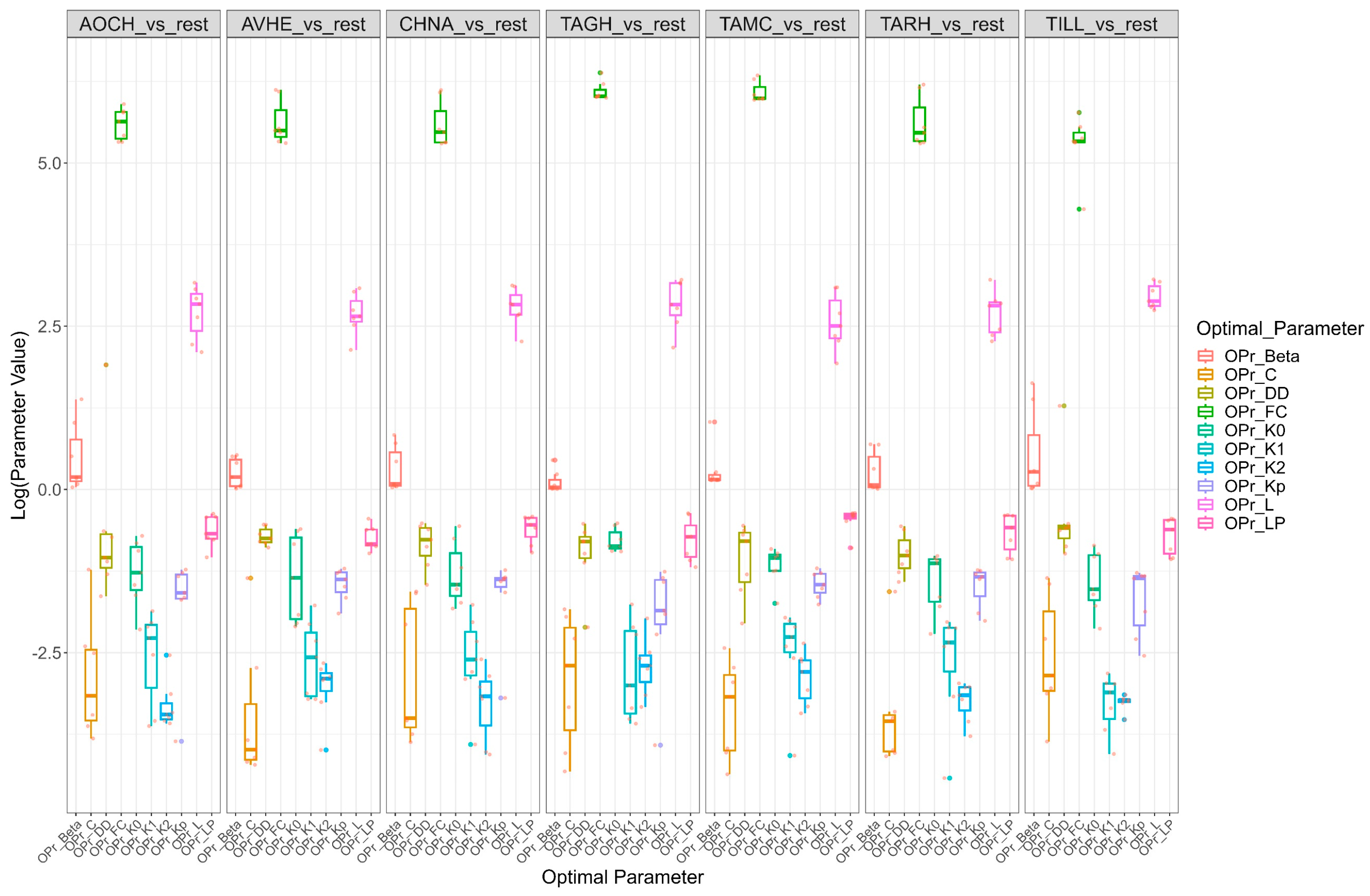
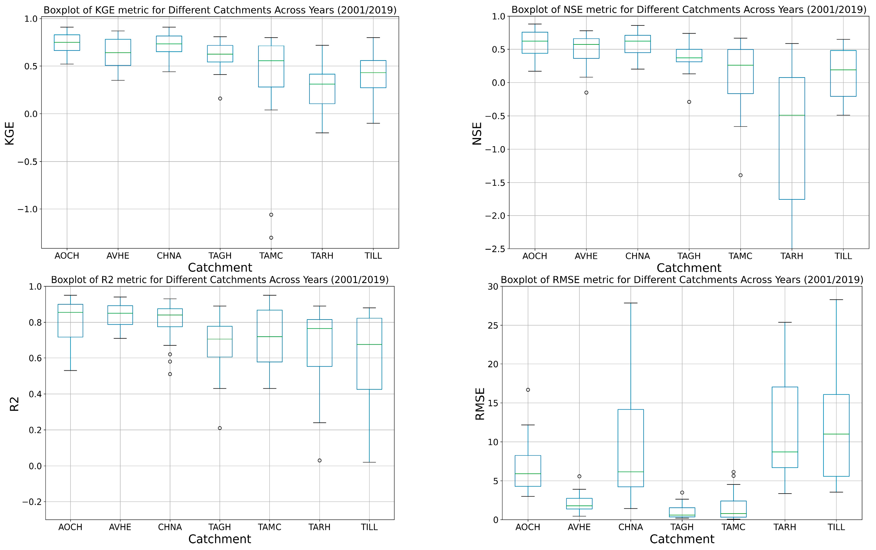
3.2.1. Spatial Stability Analysis

Maximizing the values of the KGE and NSE metrics means getting more reliable optimal parameter values to avoid output equifinality at least in terms of their representativity of the modeled system [98,110]. We determined the behavioral KGE and NSE values as the corresponding optimal parameters set with 5% of the best KGE and NSE values, from which we subsequently identified one of the corresponding optimal parameters set values as input intervals for the NCV. In this way, the optimal parameter ranges used in the target catchment are determined each time by cross-validation in the donor catchment in the form of a moving spatio-temporal window for “parameter tuning”.

The results of the NCV summarized in Figure 5 reveal that the optimal parameters and the performance metrics show a high inter-catchment variance and sometimes high positive correlation and interdependence related to each other, as in the case of optimal parameters FC, BETA, LP, L, DDF, and K0. High NSE values are usually associated with the recording of higher values of the FC and BETA optimal parameters, and this is consistent with the results reached by Beck et al. and Khazaei et al. [40,111]. This causal relationship becomes sharper as we move towards slightly better-gauged basins such as AOCH, CHNA, TAGH, and AVHE, given the precision of the in situ measurements in these basins as well as their relatively humid conditions compared to the rest of the basins (TAMC, TARH, and TILL).

We used NCV to conduct a global stability analysis and parameter tuning of a data-/process-based model across a time series of multiple inputs with relatively small time steps.

Table 4. Statistics of nested cross validation Optimal parameter sets and performances metrics of the 5% best of KGE and NSE values averaged on seven studied catchments.

Parameters	Min	Max	Avrg	StD
OPr_Beta (-)	1.0059	5.0947	1.5195	0.8602
OPr_C (mm.d−1)	0.0127	0.2930	0.0733	0.0770
OPr_DD (mm/°C.d−1)	0.1212	6.7420	0.6190	1.0098
OPr_FC (mm)	73.1931	591.1099	321.5628	121.4521
OPr_K0 (d−1)	0.1095	0.5961	0.3190	0.1368
OPr_K1 (d−1)	0.0120	0.1719	0.0811	0.0464
OPr_K2 (d−1)	0.0172	0.1389	0.0490	0.0223
OPr_Kp (mm.d−1)	0.0199	0.2990	0.2164	0.0754
OPr_L (mm)	6.8913	24.9554	16.4839	5.2186
OPr_LP (-)	0.3043	0.6982	0.5331	0.1291
Performance Metrics	Min	Max	Avrg	StD
KGE	−1.30	0.91	0.53	0.32
NSE	−0.08	0.81	0.53	0.23
R2	0.39	0.94	0.75	0.15
RMSE (m3/S)	3.83	55.32	24.96	16.48
RVE	−0.56	0.57	−0.04	0.32
AVG_NSE	−0.39	0.70	0.31	0.28

summarizes the average of the model’s ten studied optimal parameter sets and performance metrics corresponding to 5% of behavioral runs obtained after simultaneous calibration/validation periods with a moving time window of one year and a moving spatial window of one sub-catchment at a time.

Moreover, the results of maximum and minimum parameter values tend to cover the whole calibration range previously mentioned in Table 2, with typical behavior for seven optimal parameters except OPr_Beta, OPr_DDF, and OPr_FC. They recorded abnormal (out of interval) values considering their range of minimum and maximum parameter values for the calibration initially determined. This anomaly sometimes breaks the maximum values, as in the case of the OPr_Beta initial maximum = 4 and the after-NCV maximum = 5.0947. For the TILL_vs_TILL NCV-fold and OPr_DDF, the initial maximum = 0.6 mm. °C⁻¹.d⁻¹, but the after-NCV maximum = 6.7420 mm. °C⁻¹.d⁻¹ and the NCV maximum = 3.6007 mm. °C⁻¹.d⁻¹, respectively for the AOCH_vs_AOCH and TILL_vs_TILL NCV-fold. Moreover, for the minimum values, as in the case of OPr_FC, the initial minimum = 200 mm. The after-NCV minimum = 73.1931 mm for the TILL_vs_TILL (NSE = 0.1) NCV-fold. According to Merz et al. and Zhang and Lindström [80,112], the DDF, FC, and BETA parameter values are correlated and tend to decrease temporally and slightly spatially; i.e., they need as much time as possible for the temporal trend to affect the spatial trend of parameters decreasing. On the other side, OPr_C is inversely correlated to the values of K1 and K0 because of the proximity of their related reservoirs to the soil surface; the latter is mainly affected by potential evapotranspiration and evaporation and, thus, by temperature. Consequently, they are correlated negatively with most climatic variables such as (T, PET, runoff, and runoff–rainfall ratio). In Figure 5, there is a significant negative effect of OPr_C on the KGE, NSE, and Pearson coefficient values of, respectively, −0.62, −0.57, and −0.55. As seen in Figure 5, the OPr_C values have an increasing trend over time, contrary to what Merz et al. [80] concluded in their previous research. The contrast between the hydrological regime of snow-dominated mountainous catchments and flat catchments may explain this relationship. The size of the basins in the OERB upper part is smaller than those in the lower part of OERB basins, which can impact the results due to the increasing heterogeneity in hydroclimatic and physiographic features as well as land use land cover change [113,114]. Ultimately, this will become more contradictory as the temperature rises and the climatic conditions turn toward extremes since flat basins are more vulnerable than mountainous and snow-dominated ones. Furthermore, the existence of more complicated watershed processes that are not fully described by the chosen model has an impact on performance. (e.g., snowmelt or soil moisture routines in catchments with large altitude ranges or diverse land covers) [105]. Another factor to consider is that the upper part of the OERB is dominated by hydrokarstic features, which may affect model performance (since HBV considers the catchment to be a closed system) [106,107]. As a result, it is necessary to test multiple models in the same hydroclimatic context or consider using more distributed models.

Thus, the most likely reason for these anomalies is that the model requires broader parameter ranges during calibration, which stems from the spatial variability of those variables from catchment to catchment or due to the temporal variability induced by climate change and its effects. In contrast, the OPr_DDF values of TILL_vs_TILL and AOCH_vs_AOCH NCV-fold mark an increase instead of the general increasing trend (Grey bars) in Figure 5. That is possibly justified by the need to correct the OPr_DDF values to accommodate the large amounts of accumulated snow in the two sub-catchments compared to the rest of the smallest sub-catchments. Consequently, OPr_FC values also decrease and are replaced by soil moisture as the snow melts later during spring and summer as a unique feature of the TILL sub-catchment. Thus, this is clearly shown in Figure 5 since the OPr_FC (73.1931 mm) in TILL_vs_TILL has the smallest value. Hence, since parameters are mainly related to catchment characteristics [55,56], the model appears to adapt to the specific hydroclimatic conditions of the two mountainous catchments.

Despite that, the TILL catchment has the lowest performance among the seven sub-catchments, at least for NSE, RMSE, and RVE (no results of KGE shown here) and for the half of study period from (2001–2010). Therefore, we cannot match the prior findings until we re-model them with more solid hydroclimatic data for the same period. The limit for the potential evaporation (OPr_LP) parameter seems to diverge from this prevailing pattern in soil parameters of going out of the pre-determined calibration range, taking average values of 0.53 with a Std (standard deviation) = 0.13. OPr_LP also shows a negative correlation with the values of the OPr_Beta, OPr_FC, OPr_K2, and OPr_L, estimated, respectively, at −0.15, −0.24, −0.20, and −0.22. On the other hand, OPr_LP unusually shows an inverse correlation with OPr_C in AOCH, AVHE, TAGH, and TAMC and a positive correlation in the CHNA and TILL basins as water moves downward through the soil. OPr_Kp has become inversely affected by the very fast storage coefficient K0 values (R² = −0.44); this effect diminishes little by little for the fast storage coefficient K1 (0.05) and the slow storage coefficient K2 (−0.02). In our opinion, the real reason behind this atypical correlation between soil routine parameters and whether it is due to a model artifact or if the catchments are affected by recent anthropogenic activities is not evident. This matter requires a deep investigation into the characteristics of the soil routine and land use land cover dynamics in each basin and look for similarities and differences between them.

Besides the soil- and snow-related parameters, the analysis of runoff parameters, especially OPr_K0, OPr_K1, OPr_K2, OPr_KP, and OPr_UZL, gives additional insight regarding the stability of the model in terms of parameterization and accuracy across the various model routines. The model outputs in Figure 5 and their spatial variation during the spatial splitting phase in Figure 6 describe an inverse behavior between OPr_K0, OPr_K1, and OPr_Kp with OPr_L of (−0.40, −0.60, −0.40), respectively, which is normal knowing that OPr_L is the regulator of K0 and K1 and their values are inversely affected by OPr_Kp values when surface water percolate to groundwater storage. Besides, there is a direct-to-moderate positive correlation between OPr_K0 and OPr_K1 value changes and KGE, NSE, R², and RMSE performance metrics, while this correlation becomes slightly negative for RVE values. The latter seems to be significantly affected by OPr_Kp values (0.45). We infer from the former that decreased streamflow may be caused by low rainfall (particularly snowfall), low antecedent soil moisture, high temperatures and evaporation rates, or issues with water distribution. Given that the flows through the soil layers may increase the model’s vertical inaccuracy as well as the horizontal passing from one sub-catchment to another, this is consistent with different research findings of [80,99,108,109].

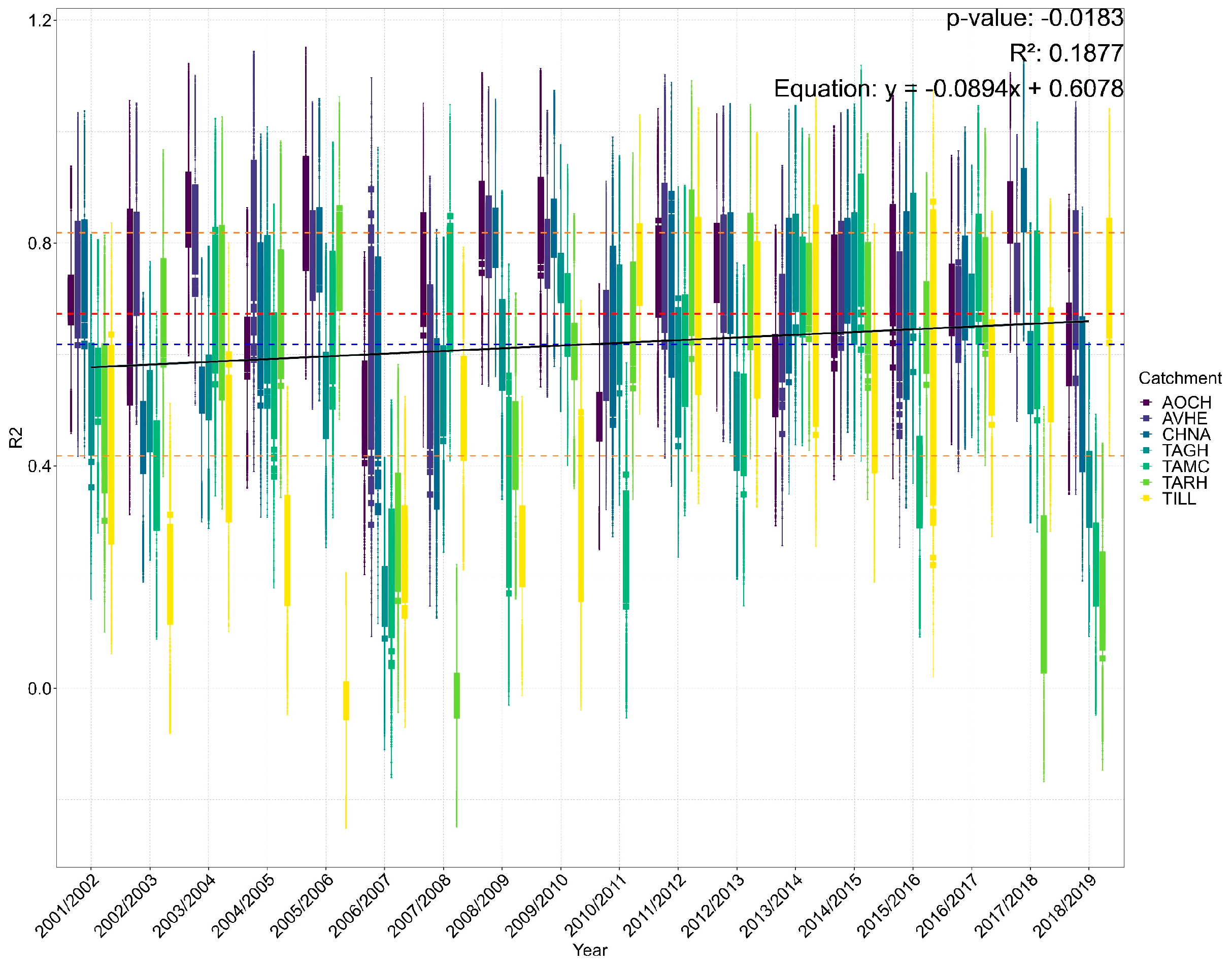
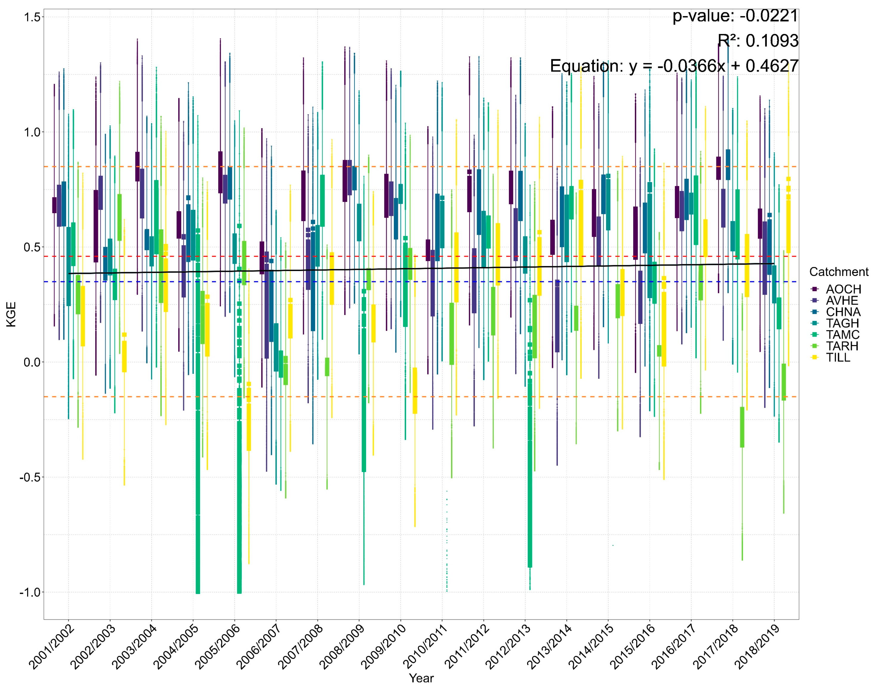
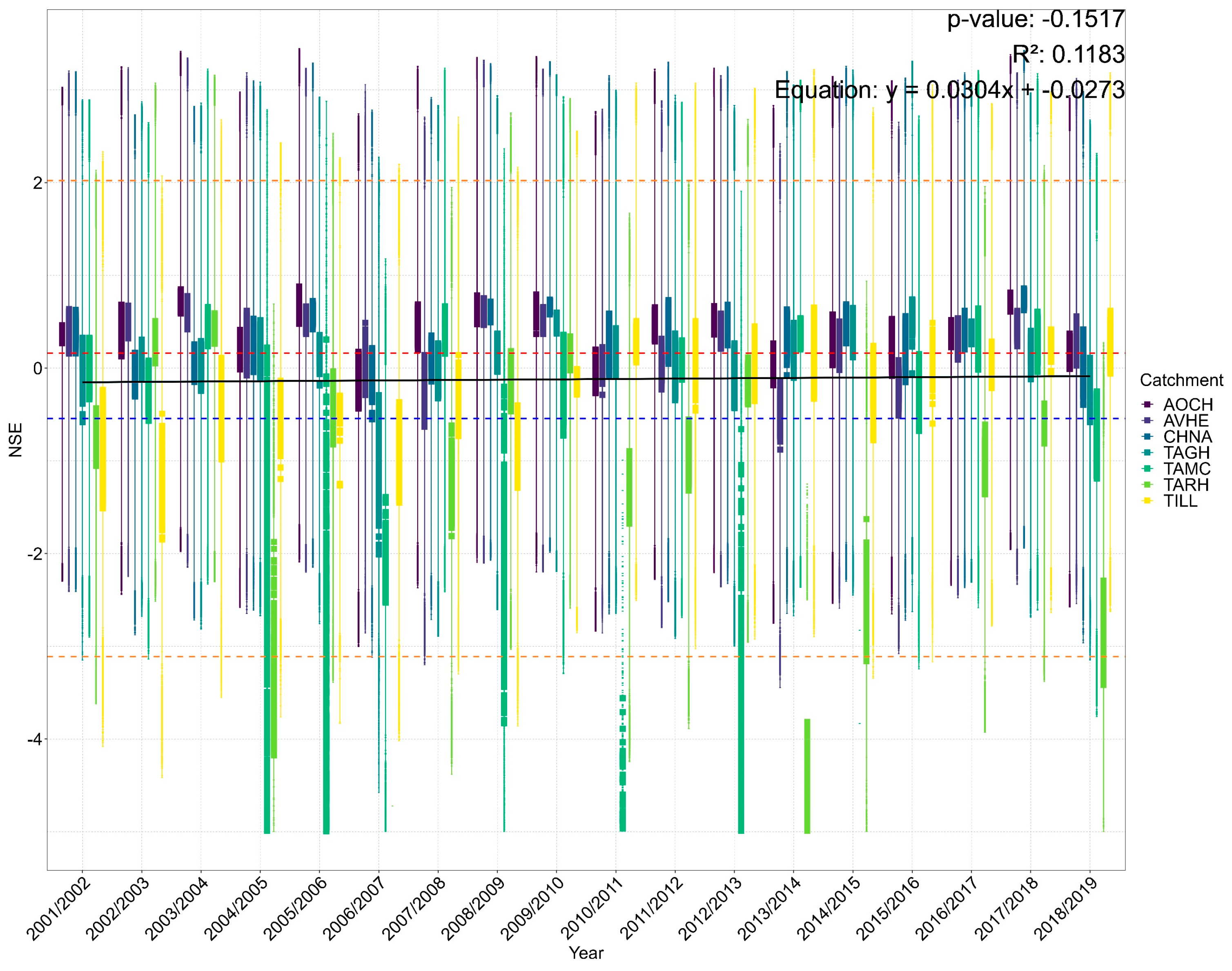
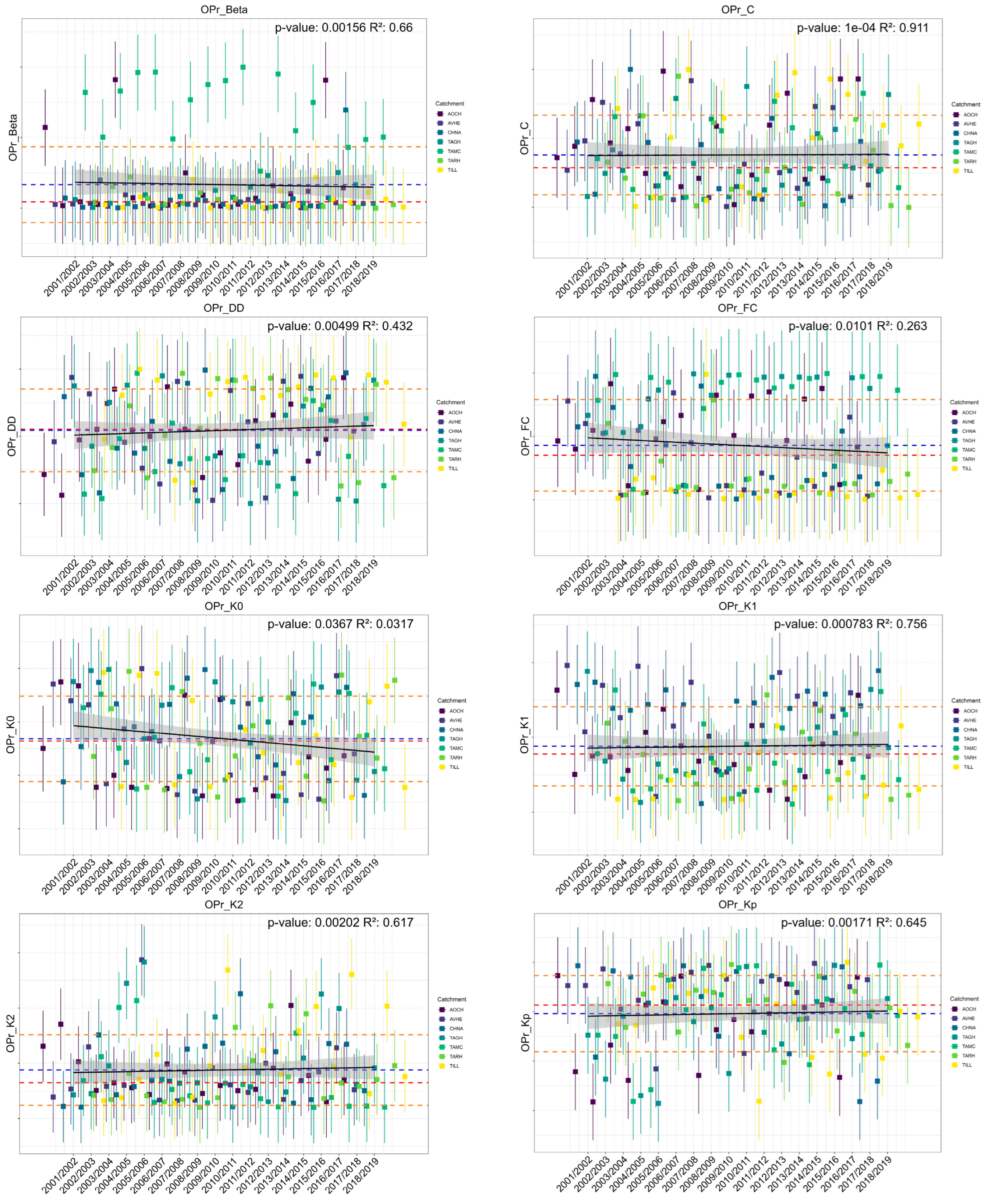
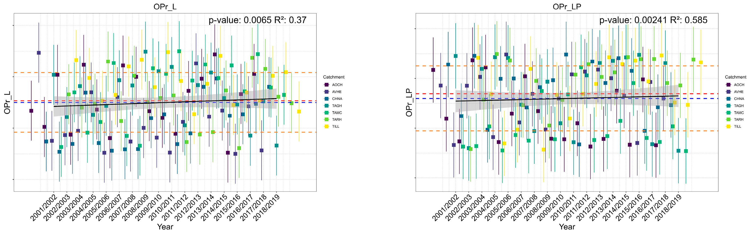
3.2.2. Temporal Stability Analysis

The stability of the model over time was done through a one-year time splitting of data using cross-validation, then allocating a year for calibration and the rest of the years for validation. The analysis of NCV results suggests significant changes and trends in the model parameters and performance metrics between 2001 and 2019. R² in Appendix A marks the sharpest increasing trend over time, with a p-value = −0.0183. In general, R² quantifies the overall fit without considering cases of over- or underestimation by the model. So, in our opinion, there are long-term improvements in gauging station data quality that justify the increasing trend in R², as we observe this when working with the data especially the TARH and TILL catchment; and as we head towards the year 2018/2019, we notice an improvement in the linear correlation values between precipitations and streamflow; otherwise, this may also be evidence of the effectiveness of the calibration strategy.

Otherwise, the KGE, NSE, RMSE, and RVE metrics show an overall decline across the study period, which indicates a model’s performance decreasing throughout the seven sub-catchments evaluated.

On a more detailed level, the dumbbell plot of R² (Appendix A) values over time and space showed a high ability of the metric to capture the hydrological behavior for each year. Drought years coincide with a severe decline in R² values in TAGH, TAMC, TARH, and TILL basins during the years 2001/2002, 2002/2003, 2006/2007, 2007/2008, 2010/2011, 2015/2016, and 2018/2019. In 11 years out of the 18, the R² efficiency values in the TILL sub-catchment are below or in the lower quartile (Q1), while the TAMC’s R² values are below or in the lower quartile (Q1) in 9 out of 18 years. The dumbbell plot of KGE and NSE (Figure 7 and Figure 8) values over time and space shows unique behavior for the TAMC sub-catchment (KGE) and TAMC and TARH sub-catchments (for NSE); it appears to be highly sensitive to time change, as the model loses its performance significantly in this sub-basin year after year, particularly in dry years such as (2004/2005, 2005/2006, 2010/2011, 2012/2013, and 2014/2015); conversely, the remaining sub-catchments recorded a periodic behavior of mean KGE values (KGE = 0.57) that fluctuated between good to moderate performances depending on whether the period was dry or wet. Based on our analysis of the hydrological history of the seven sub-catchments and the findings of [22], we can confirm that NSE was able to better catch drought years as in the case of the TARH sub-catchment for the hydrologic years 2004/2005, 2006/2007, 2013/2014, 2014/2015, and 2015/2016. Otherwise, the RMSE patterns in Figure 9 behave differently over time, with high RMSE values coinciding with wet years, as shown in Figure 10, thus indicating how wet the year was and whether the basin in question has received significant amounts of precipitation, regardless of KGE and NSE accuracy.

Studying model parameter trends and patterns, as well as their changes over time, is considered an essential basis for the model stability of the hydroclimatic and physiographic features of the basins. It also gives an overview of the most influential model components, thus contributing to the facility of analysis and understanding of reasons for those trends and predict their condition in the future. Figure 11 resumes the ten HBV optimal parameter trends over 18 years of study. The values of two soil-related parameters, OPr_Beta and OPr_FC, in addition to one runoff-related parameter, OPr_K0, showed a decreased trend across the study period. In the OPr_Beta dumbbell plot (Figure 11), catchments are of two groups, according to the BETA values during the study period [43]. The AOCH and TAMC groups’ sub-catchments often fall in the interval of values greater than 0.5, whereas the second group consists of the rest of the eight parameters with values mostly centered around the median and much lower than the average. There was a slight increase in the trend of OPr_C as a snow temperature conditions witness regarding the inter-annual and inter-catchment change in OPr_C values, which records marked inter-annual oscillation where dry years and basins are recording higher values of temperature correction factor OPr_C. Ouyang et al. [85] argued that this parameter is constant in time because it is not activated significantly except in important snow events, which are scarce in our case of an arid to semi-arid context. Reversely, the OPr_DD trend increases over time in half of the catchments characterized by low to medium performances (TAMC, TARH, TILL), while the values of OPr_DD are a decreasing trend in the rest of the catchments, which may indicate a partial shift in the prevailing climate within. Evapotranspiration, represented by OPr_LP, would be expected to increase because of the significant increase in air temperatures.

Another impactful parameter in the HBV model response is the field capacity OPr_FC. It has a decreasing trend during the study period, and generally, a clear distinction between catchments with high FC values (AOCH, TAGH, and TAMC) and those with small values (AVHE, CHNA, TARH, and TILL). This distinction of catchments occurred without any effect on model performance within. According to the findings of Kavetski et al. and Ouyang et al. [85,110], the FC is supposed to be relatively stable over time. Hence, the long-term changes observed in the FC trend can only be because of changes in the physiographic characteristics of the studied sub-catchments, especially a slope-based division of catchments and a reduction in OPr_FC in favor of OPr_K1 in case of high slope catchments [111], or it may indicate the tendency of the studied catchments toward low flow conditions due to climate change [85], which is also a valid discussion for OPr_Kp, OPr_K1, OPr_K2, OPr_L, and OPr_LP that tend toward upward trends. In the same context, Niel et al. [112] conclude that there is no correlation between the parameter stability, and the invariant behavior of rainfall and runoff data series for some catchments. The results of Merz et al. [80] using 30 years of data from 273 catchments over Austria and a semi-distributed model across various periods can be used to support Niel’s claim since they noted that some model parameters are stationary and had a doubling trend over time, somewhat similar to the climatic conditions changes trend in the study area between the past and the present.

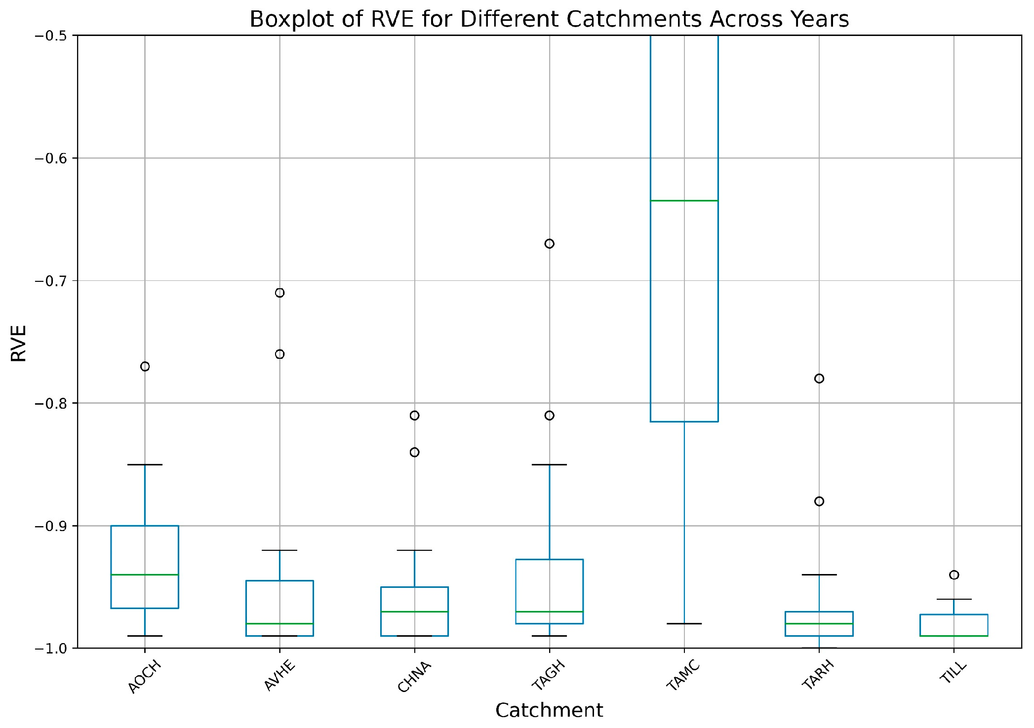
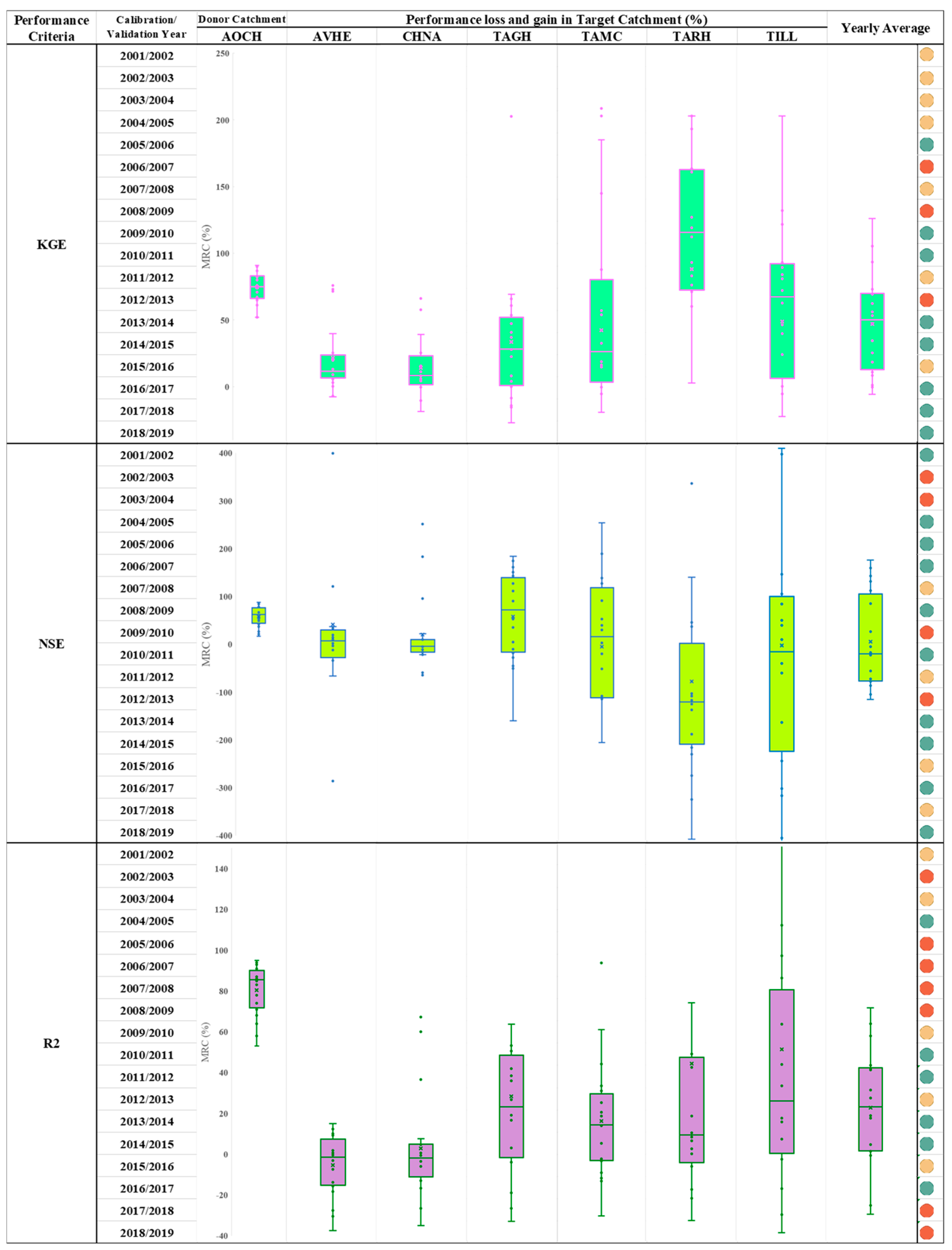
3.3. Performance Loss Analysis

An important consideration is to quantify and understand whether these trends in optimal parameters can impact model performance and stability over time and space and whether climatic variability could explain it. The data in Figure 12 represent the performance losses and gains of the HBV model in the target watersheds as a function of different calibration/validation years for each of the three efficiency performance criteria: NSE, KGE, and R² coefficient. The MRC values are ratios of losses and gains of post-calibration/verification efficiency measures between the donor basin (AOCH) and the next target basin to show the effect of the optimal parameter’s regionalization on the stability and efficiency of the model.

Overall, in Figure 12, there is a mixture of positive and negative MRC values for the KGE, NSE, and R² across the years and catchments. Generally, for the KGE metric, negative MRC values suggest a performance improvement against AOCH performances (minimum of MRC gain = −200% in TARH and TILL, a maximum MRC gain = −2% in CHNA, and yearly average ranges between −6% in 2009/2010 and −13% in 2010/2011) when transferring parameter sets from donor to target catchments and periods. There were notable instances in 2005/2006, 2009/2010, 2010/2011, 2017/2018, and 2018/2019 in various catchments such as CHNA, TAGH, and TARH/TILL in some wet years. Positive MRC values, on the other hand, indicate performance losses and difficulty in transferring calibrated parameter sets, thus model instability. Performance losses have been noted over multiple hydrologic years, including 2002/2003 (minimum of MRC loss = 2%), 2006/2007 2007/2008, 2008/2009 (maximum of MRC loss = 260%), 2011/2012, 2012/2013, 2015/2016, and 2018/2019 mostly, in the TARH and TILL catchments.

Similarly, NSE and R² have both positive and negative MRC values. There was significant accuracy deterioration in catchments experiencing positive losses. Those MRC loss values range between a maximum of 762% (in TAMC, 2002/2003) and 9% (in TILL, in 2015/2016) of minimum loss, mainly in AVHE, TAMC, TARH, and TILL for the years 2004/2005, 2005/2006, 2007/2008, 2008/2009, 2015/2016, and 2018/2019. Significant performance gains are notable in 2007/2008 for several catchments, but losses are observed in 2006/2007 and 2013/2014, especially in AOCH and AVHE. Negative MRC values indicate performance losses, showing the transferring difficulties of calibrated parameter sets. In terms of the R² metric, substantial performance increases are apparent in 2006/2007 for the AVHE and CHNA catchments, although general performance gain occurs in other years, such as 2010/2011, 2013/2014, and, relatively, 2004/2005 and 2014/2015. The R² performance looks more consistent than KGE and NSE regarding cases of performance loss or gain when passing from donor to target catchment, as it shows in some cases the same pattern in most basins inter-annually.

As stated by Coron et al. and Ji et al. [98,113], a higher performance loss is a result of contrasting climate variables (mainly average rainfall and evapotranspiration) between donor and target catchments, especially when donor catchment or periods are wetter than target ones. Furthermore, the results of the adopted approach reinforce what Coron et al. [98] concluded, which is that any change in the mean rainfall reduces the transferability of optimal parameters. Hence, model stability decreases, especially from dry to wet periods, since this conclusion also remains valid in the case of parameters regionalization from a dry catchment to another wet catchment, as in the case of AOCH with the rest of the studied catchments except the drier one (TILL).

The last column of the yearly mean model robustness criterion (MRC), shown in Figure 12, gives a general aspect of the trends in Figure 13 of three main performance metrics: KGE, NSE, and R². The analysis of the KGE and NSE MRC trends in Figure 13 suggests that the average annual MRC of KGE and NSE indicates the overall transferability of optimized parameter sets from donor to target catchment. The figure also shows a succession of periods of high loss of efficiency and others of low loss. These periods span an average of five years, corresponding to the drought episodes recorded over the study period [114].

Otherwise, a general look at the KGE, NSE, and R² MRC trend slope, for at least the period between 2001/2002 and 2018/2019, suggests that the model is improving in robustness through time and space. In addition, the trend curve of performance loss for KGE differs from that of NSE in that the latter records a succession over shorter periods than KGE, implying that it is more sensitive than KGE to hydroclimatic conditions changes, whether towards drought or wetness. Similarly, R² seems to be more lumped than KGE and NSE in terms of sensitivity to the oscillation in trend between dry and wet periods, as it records just two periods of increasing trend of MRC values from 2001/2002 to 2009/2010, then a slightly decreasing period starting from 2010/2011 to the end of 2019, where another rise of performance loss began.

4. Conclusions

During this work, we tested the structure stability of the HBV conceptual model, as well as its performances in an arid to semi-arid and poorly gauged climate context, through a systematic construction of a modeling platform that simultaneously simulates and measures the stability of the HBV model in time and space. Over 18 years, the study focused on modeling seven of the most critical sub-catchments of the Oum Er Rabia river basin in central Morocco. Ait Ouchene was adopted alternately as a donor basin of optimal parameters, while the rest were targets. Then, we reproduced the flow in the seven basins, using in situ, satellite, and reanalysis data and the nested cross-calibration/validation technique simultaneously to split data in time and space. After the cross-validation of the HBV model, we kept the generated optimal parameter sets and their related performance metrics. These data are the raw material to analyze and test the spatiotemporal model stability in terms of accuracy and optimal parameter values.

The findings reveal that the HBV model remains spatially transferable from one basin to another with moderate to high performances of KGE (0.1~0.9), NSE (0.5~0.8), R² (0.6~0.9), and RMSE (2~27.2) metrics. However, flow underestimation occurs, especially in contexts with inadequate representation of snowmelt dynamics. Besides, HBV optimal parameter sets exhibit unstable behavior over space, with a typical behavior for seven optimal parameters except for OPr_Beta, OPr_DDF, and OPr_FC because they recorded out-of-interval values considering their ranges of variation initially determined. On the contrary, their inter-annual behavior in AOCH is nearly constant, and the intra-annual behavior marks an oscillation between dry and wet periods. A model performance improvement is also registered when adding KGE to the calibration toolkit.

Despite this, in the TILL catchment, the model’s poor performance (NSE = 0.14, KGE = 0.29) was linked to its inability to capture the hydrological processes associated with bare soils, which promote infiltration and subsurface flows, leading to underestimation of runoff. Additionally, karstic systems in the upper Oum Er Rabia basin further complicate runoff generation, as the HBV model does not account for complex surface–subsurface interactions, resulting in poor low-flow simulations. These biases, along with increased RMSE values, suggest that the model struggles with peak flow sensitivity, especially in regions with inter-annual variability in precipitation. The model’s inability to capture low flows in dry seasons, critical for water resource management in semi-arid areas, reflects its limitations in accounting for spatial rainfall variability and flow transmission losses common in such regions.

The spatial stability investigation using nested cross-calibration and validation demonstrates significant inter-catchment variation in optimal parameters and performance metrics, notably for the FC and BETA parameters. While the model responds effectively to specific hydroclimatic conditions, anomalies in parameter values indicate the need for wider parameter ranges during calibration, which might be impacted by spatial and temporal variability caused by climate change.

Furthermore, analyzing runoff parameters gives insights into the model’s stability and accuracy across different model routines, emphasizing the relevance of knowing the hydrological processes that influence streamflow.

Moreover, the analysis of model parameter trends reveals notable patterns, such as the declining trend of some soil-related indices such as OPr_Beta and OPr_FC, indicating probable changes in physiographic features and hydrological conditions within the catchments. Furthermore, the declining trend in field capacity (OPr_FC) may be a reaction to changing climatic conditions, highlighting the necessity of knowing long-term hydroclimatic trends for accurate modeling.

Finally, the analysis of model performance loss over time highlights significant trends in performance metrics across the study period, with R² showing a sharply increasing trend while other metrics like KGE, NSE, RMSE, and RVE demonstrate an overall decline (between 2% to 103% for KGE, between 25% to 171% for NSE, and 1% to 73% for R²) of the model’s predictive capabilities with time. We assume that the cause of the performance loss trend of the HBV model is the tendency of the climate in the study area toward dryness year after year.

The novelty of this framework, in addition to the simplicity of the chosen model and approach, lies in the fact of not neglecting the time component at the expense of space or vice versa. It also provides a convenient tool to benefit as much as possible from hydroclimatic time series—despite the data scarcity and poor quality—because of the use of accessible remotely sensed data and the cross-validation technique. The latter is considered an effective tool to cover most of the duration of the time series of hydroclimatic variables for both calibration and validation periods. However, additional research must be done to better understand the interaction between the spatial and temporal factors influencing watershed hydrological variability, such as the time step of calibration and validation, the most affected components of the water cycle, and finally, the relevance of satellite against in situ data.

References

1. Burek, P.; Satoh, Y.; Fischer, G.; Kahil, M.T.; Scherzer, A.; Tramberend, S.; Nava, L.F.; Wada, Y.; Eisner, S.; Flörke, M. Water Futures and Solution—Fast Track Initiative; IIASA Working Paper; IIASA: Laxenburg, Austria, 2016. [Google Scholar]
2. World Water Assessment Programme. The United Nations World Water Development Report 2018; United Nations Educational, Scientific and Cultural Organization: New York, NY, USA, 2018. [Google Scholar]
3. Chai, T.; Draxler, R.R. Root Mean Square Error (RMSE) or Mean Absolute Error (MAE)?—Arguments against Avoiding RMSE in the Literature. Geosci. Model Dev. 2014, 7, 1247–1250. [Google Scholar] [CrossRef]
4. Hoekstra, A.Y. Water Scarcity Challenges to Business. Nat. Clim. Chang. 2014, 4, 318–320. [Google Scholar] [CrossRef]
5. Water Consumption BT. Clean Water and Sanitation; Leal Filho, W., Azul, A.M., Brandli, L., Lange Salvia, A., Wall, T., Eds.; Springer International Publishing: Cham, Switzerland, 2022; p. 774. ISBN 978-3-319-95846-0. [Google Scholar]
6. Richter, B.D.; Bartak, D.; Caldwell, P.; Davis, K.F.; Debaere, P.; Hoekstra, A.Y.; Li, T.; Marston, L.; McManamay, R.; Mekonnen, M.M.; et al. Water Scarcity and Fish Imperilment Driven by Beef Production. Nat. Sustain. 2020, 3, 319–328. [Google Scholar] [CrossRef]
7. Dalezios, N.R.; Angelakis, A.N.; Eslamian, S. Water Scarcity Management: Part 1: Methodological Framework. Int. J. Glob. Environ. Issues 2018, 17, 1–40. [Google Scholar] [CrossRef]
8. Tzanakakis, V.A.; Paranychianakis, N.V.; Angelakis, A.N. Water Supply and Water Scarcity. Water 2020, 12, 2347. [Google Scholar] [CrossRef]
9. Boretti, A.; Rosa, L. Reassessing the Projections of the World Water Development Report. NPJ Clean Water 2019, 2, 15. [Google Scholar] [CrossRef]
10. OECD. OECD Environmental Outlook to 2050; OECD: Paris, France, 2012; ISBN 9789264122161. [Google Scholar]
11. Pokhrel, Y.; Felfelani, F.; Satoh, Y.; Boulange, J.; Burek, P.; Gädeke, A.; Gerten, D.; Gosling, S.N.; Grillakis, M.; Gudmundsson, L.; et al. Global Terrestrial Water Storage and Drought Severity under Climate Change. Nat. Clim. Change 2021, 11, 226–233. [Google Scholar] [CrossRef]
12. Tramblay, Y.; Jarlan, L.; Hanich, L.; Somot, S. Future Scenarios of Surface Water Resources Availability in North African Dams. Water Resour. Manag. 2018, 32, 1291–1306. [Google Scholar] [CrossRef]
13. Tzanakakis, V.A.; Angelakis, A.N.; Paranychianakis, N.V.; Dialynas, Y.G.; Tchobanoglous, G. Challenges and Opportunities for Sustainable Management of Water Resources in the Island of Crete, Greece. Water 2020, 12, 1538. [Google Scholar] [CrossRef]
14. Bates, B.; Kundzewicz, Z.; Wu, S. Climate Change and Water; Intergovernmental Panel on Climate Change Secretariat: Geneva, Switzerland, 2008; ISBN 9291691232. [Google Scholar]
15. Driouech, F.; ElRhaz, K.; Moufouma-Okia, W.; Arjdal, K.; Balhane, S. Assessing Future Changes of Climate Extreme Events in the CORDEX-MENA Region Using Regional Climate Model ALADIN-Climate. Earth Syst. Environ. 2020, 4, 477–492. [Google Scholar] [CrossRef]
16. Keshav, S. How to Read a Paper. ACM SIGCOMM Comput. Commun. Rev. 2007, 37, 83–84. [Google Scholar] [CrossRef]
17. Noto, L.V.; Cipolla, G.; Francipane, A.; Pumo, D. Climate Change in the Mediterranean Basin (Part I): Induced Alterations on Climate Forcings and Hydrological Processes. Water Resour. Manag. 2022, 37, 2287–2305. [Google Scholar] [CrossRef]
18. Pellet, V.; Aires, F.; Munier, S.; Fernández Prieto, D.; Jordá, G.; Dorigo, W.A.; Polcher, J.; Brocca, L. Integrating Multiple Satellite Observations into a Coherent Dataset to Monitor the Full Water Cycle—Application to the Mediterranean Region. Hydrol. Earth Syst. Sci. 2019, 23, 465–491. [Google Scholar] [CrossRef]
19. Rochdane, S.; Reichert, B.; Messouli, M.; Babqiqi, A.; Khebiza, M.Y. Climate Change Impacts on Water Supply and Demand in Rheraya Watershed (Morocco), with Potential Adaptation Strategies. Water 2012, 4, 28–44. [Google Scholar] [CrossRef]
20. Voss, R.; May, W.; Roeckner, E. Enhanced Resolution Modelling Study on Anthropogenic Climate Change: Changes in Extremes of the Hydrological Cycle. Int. J. Climatol. 2002, 22, 755–777. [Google Scholar] [CrossRef]
21. Marchane, A.; Tramblay, Y.; Hanich, L.; Ruelland, D.; Jarlan, L. Climate Change Impacts on Surface Water Resources in the Rheraya Catchment (High Atlas, Morocco). Hydrol. Sci. J. 2017, 62, 979–995. [Google Scholar] [CrossRef]
22. Boudhar, A.; Baba, W.M.; Marchane, A.; Ouatiki, H.; Bouamri, H.; Hanich, L.; Chehbouni, A. Water Resources Monitoring Over the Atlas Mountains in Morocco Using Satellite Observations and Reanalysis Data BT. In Remote Sensing of African Mountains: Geospatial Tools toward Sustainability; Adelabu, S., Ramoelo, A., Olusola, A., Adagbasa, E., Eds.; Springer International Publishing: Cham, Switzerland, 2022; pp. 157–170. ISBN 978-3-031-04855-5. [Google Scholar]
23. Zittis, G.; Bruggeman, A.; Lelieveld, J. Revisiting Future Extreme Precipitation Trends in the Mediterranean. Weather Clim. Extrem. 2021, 34, 100380. [Google Scholar] [CrossRef]
24. Sidle, R.C. Strategies for Smarter Catchment Hydrology Models: Incorporating Scaling and Better Process Representation. Geosci. Lett. 2021, 8, 24. [Google Scholar] [CrossRef]
25. Aghakouchak, A.; Habib, E. Application of a Conceptual Hydrologic Model in Teaching Hydrologic Processes. Int. J. Eng. Educ. 2010, 26, 963–973. [Google Scholar]
26. Coopersmith, E.; Yaeger, M.A.; Ye, S.; Cheng, L.; Sivapalan, M. Exploring the Physical Controls of Regional Patterns of Flow Duration Curves—Part 3: A Catchment Classification System Based on Regime Curve Indicators. Hydrol. Earth Syst. Sci. 2012, 16, 4467–4482. [Google Scholar] [CrossRef]
27. Devia, G.K.; Ganasri, B.P.; Dwarakish, G.S. A Review on Hydrological Models. Aquat. Procedia 2015, 4, 1001–1007. [Google Scholar] [CrossRef]
28. Duan, Q.; Sorooshian, S.; Gupta, V. Effective and Efficient Global Optimization for Conceptual Rainfall-runoff Models. Water Resour. Res. 1992, 28, 1015–1031. [Google Scholar] [CrossRef]
29. Clark, M.P.; Kavetski, D.; Fenicia, F. Pursuing the Method of Multiple Working Hypotheses for Hydrological Modeling. Water Resour. Res. 2011, 47, W09301. [Google Scholar] [CrossRef]
30. Singh, V.P. Hydrologic Modeling: Progress and Future Directions. Geosci. Lett. 2018, 5, 15. [Google Scholar] [CrossRef]
31. Krysanova, V.; Donnelly, C.; Gelfan, A.; Gerten, D.; Arheimer, B.; Hattermann, F.; Kundzewicz, Z.W. How the Performance of Hydrological Models Relates to Credibility of Projections under Climate Change. Hydrol. Sci. J. 2018, 63, 696–720. [Google Scholar] [CrossRef]
32. Bergstrom, S. Experience from Applications of the HBV Hydrological Model from the Perspective of Prediction in Ungauged Basins. IAHS Publ. 2006, 307, 97. [Google Scholar]
33. Bouadila, A.; Tzoraki, O.; Benaabidate, L. Hydrological Modeling of Three Rivers under Mediterranean Climate in Chile, Greece, and Morocco: Study of High Flow Trends by Indicator Calculation. Arab. J. Geosci. 2020, 13, 1057. [Google Scholar] [CrossRef]
34. Ouachani, R.; Bargaoui, Z.; Ouarda, T. Integration of a Kalman Filter in the HBV Hydrological Model for Runoff Forecasting. Hydrol. Sci. J. 2007, 52, 318–337. [Google Scholar] [CrossRef]
35. Ouatiki, H.; Boudhar, A.; Ouhinou, A.; Beljadid, A.; Leblanc, M.; Chehbouni, A. Sensitivity and Interdependency Analysis of the HBV Conceptual Model Parameters in a Semi-Arid Mountainous Watershed. Water 2020, 12, 2440. [Google Scholar] [CrossRef]
36. Seibert, J.; Beven, K.J. Gauging the Ungauged Basin: How Many Discharge Measurements Are Needed? Hydrol. Earth Syst. Sci. 2009, 13, 883–892. [Google Scholar] [CrossRef]
37. Vrochidou, A.-E.K.; Tsanis, I.K.; Grillakis, M.G.; Koutroulis, A.G. The Impact of Climate Change on Hydrometeorological Droughts at a Basin Scale. J. Hydrol. 2013, 476, 290–301. [Google Scholar] [CrossRef]
38. Seibert, J.; Bergström, S. A Retrospective on Hydrological Catchment Modelling Based on Half a Century with the HBV Model. Hydrol. Earth Syst. Sci. 2022, 26, 1371–1388. [Google Scholar] [CrossRef]
39. Arheimer, B.; Lindström, G. Climate Impact on Floods: Changes in High Flows in Sweden in the Past and the Future (1911–2100). Hydrol. Earth Syst. Sci. 2015, 19, 771–784. [Google Scholar] [CrossRef]
40. Khazaei, M.R.; Heidari, M.; Shahid, S.; Hasirchian, M. Consideration of Climate Change Impacts on a Hydropower Scheme in Iran. Theor. Appl. Climatol. 2024, 155, 3119–3132. [Google Scholar] [CrossRef]
41. Kundzewicz, Z.W.; Mata, L.J.; Arnell, N.W.; Doll, P.; Kabat, P.; Jimenez, B.; Miller, K.; Oki, T.; Zekai, S.; Shiklomanov, I. Freshwater Resources and Their Management. In Climate Change 2007: Impacts, Adaptation and Vulnerability. Contribution of Working Group II to the Fourth Assessment Report of the Intergovernmental Panel on Climate Change; Cambridge University Press: Cambridge, UK, 2007. [Google Scholar]
42. Xu, C.-Y. Estimation of Parameters of a Conceptual Water Balance Model for Ungauged Catchments. Water Resour. Manag. 1999, 13, 353–368. [Google Scholar] [CrossRef]
43. Dakhlaoui, H.; Ruelland, D.; Tramblay, Y.; Bargaoui, Z. Evaluating the Robustness of Conceptual Rainfall-Runoff Models under Climate Variability in Northern Tunisia. J. Hydrol. 2017, 550, 201–217. [Google Scholar] [CrossRef]
44. Giorgi, F.; Lionello, P. Climate Change Projections for the Mediterranean Region. Glob. Planet. Change 2008, 63, 90–104. [Google Scholar] [CrossRef]
45. Blöschl, G.; Montanari, A. Climate Change Impacts—Throwing the Dice? Hydrol. Process. Int. J. 2010, 24, 374–381. [Google Scholar] [CrossRef]
46. Mao, G.; Wang, M.; Liu, J.; Wang, Z.; Wang, K.; Meng, Y.; Zhong, R.; Wang, H.; Li, Y. Comprehensive Comparison of Artificial Neural Networks and Long Short-Term Memory Networks for Rainfall-Runoff Simulation. Phys. Chem. Earth Parts A/B/C 2021, 123, 103026. [Google Scholar] [CrossRef]
47. Parajka, J.; Blöschl, G.; Merz, R. Regional Calibration of Catchment Models: Potential for Ungauged Catchments. Water Resour. Res. 2007, 43, W06406. [Google Scholar] [CrossRef]
48. Guo, Y.; Zhang, Y.; Zhang, L.; Wang, Z. Regionalization of Hydrological Modeling for Predicting Streamflow in Ungauged Catchments: A Comprehensive Review. WIREs Water 2021, 8, e1487. [Google Scholar] [CrossRef]
49. Kokkonen, T.S.; Jakeman, A.J.; Young, P.C.; Koivusalo, H.J. Predicting Daily Flows in Ungauged Catchments: Model Regionalization from Catchment Descriptors at the Coweeta Hydrologic Laboratory, North Carolina. Hydrol. Process. 2003, 17, 2219–2238. [Google Scholar] [CrossRef]
50. McIntyre, N.; Lee, H.; Wheater, H.; Young, A.; Wagener, T. Ensemble Predictions of Runoff in Ungauged Catchments. Water Resour. Res. 2005, 41, W12434. [Google Scholar] [CrossRef]
51. Mosley, M.P. Delimitation of New Zealand Hydrologic Regions. J. Hydrol. 1981, 49, 173–192. [Google Scholar] [CrossRef]
52. Riggs, H.C. Low-Flow Investigations; US Government Printing Office: Washington, DC, USA, 1972.
53. Song, Z.; Xia, J.; Wang, G.; She, D.; Hu, C.; Hong, S. Regionalization of Hydrological Model Parameters Using Gradient Boosting Machine. Hydrol. Earth Syst. Sci. 2022, 26, 505–524. [Google Scholar] [CrossRef]
54. Blöschl, G.; Sivapalan, M. Scale Issues in Hydrological Modelling: A Review. Hydrol. Process. 1995, 9, 251–290. [Google Scholar] [CrossRef]
55. Seibert, J. Regionalisation of Parameters for a Conceptual Rainfall-Runoff Model. Agric. For. Meteorol. 1999, 98–99, 279–293. [Google Scholar] [CrossRef]
56. Beck, H.E.; Pan, M.; Lin, P.; Seibert, J.; van Dijk, A.I.J.M.; Wood, E.F. Global Fully Distributed Parameter Regionalization Based on Observed Streamflow From 4,229 Headwater Catchments. J. Geophys. Res. Atmos. 2020, 125, e2019JD031485. [Google Scholar] [CrossRef]
57. Garambois, P.A.; Roux, H.; Larnier, K.; Labat, D.; Dartus, D. Parameter Regionalization for a Process-Oriented Distributed Model Dedicated to Flash Floods. J. Hydrol. 2015, 525, 383–399. [Google Scholar] [CrossRef]
58. Li, H.; Zhang, Y.; Chiew, F.H.S.; Xu, S. Predicting Runoff in Ungauged Catchments by Using Xinanjiang Model with MODIS Leaf Area Index. J. Hydrol. 2009, 370, 155–162. [Google Scholar] [CrossRef]
59. Oudin, L.; Andréassian, V.; Perrin, C.; Michel, C.; Le Moine, N. Spatial Proximity, Physical Similarity, Regression and Ungaged Catchments: A Comparison of Regionalization Approaches Based on 913 French Catchments. Water Resour. Res. 2008, 44, W03413. [Google Scholar] [CrossRef]
60. Parajka, J.; Merz, R.; Blöschl, G. A Comparison of Regionalisation Methods for Catchment Model Parameters. Hydrol. Earth Syst. Sci. 2005, 9, 157–171. [Google Scholar] [CrossRef]
61. Reichl, J.P.C.; Western, A.W.; McIntyre, N.R.; Chiew, F.H.S. Optimization of a Similarity Measure for Estimating Ungauged Streamflow. Water Resour. Res. 2009, 45, W10423. [Google Scholar] [CrossRef]
62. Singh, R.; Archfield, S.A.; Wagener, T. Identifying Dominant Controls on Hydrologic Parameter Transfer from Gauged to Ungauged Catchments–A Comparative Hydrology Approach. J. Hydrol. 2014, 517, 985–996. [Google Scholar] [CrossRef]
63. Gupta, H.V.; Nearing, G.S. Debates-the Future of Hydrological Sciences: A (Common) Path Forward? Using Models and Data to Learn: A Systems Theoretic Perspective on the Future of Hydrological Science. Water Resour. Res. 2014, 50, 5351–5359. [Google Scholar] [CrossRef]
64. Boudhar, A.; Hanich, L.; Boulet, G.; Outaleb, K.; Arioua, A.; Ben, B.; Hakkani, B. Etude de La Disponibilité Des Ressources En Eau à l’aide de La Télédétection et La Modélisation: Cas Du Bassin Versant d’Oum Er Rbia (Maroc). In Proceedings of the 3éme Colloque International Eau-Climat, Hammamet, Tunisia, 21–23 October 2014. [Google Scholar]
65. Strohmeier, S.; López López, P.; Haddad, M.; Nangia, V.; Karrou, M.; Montanaro, G.; Boudhar, A.; Linés, C.; Veldkamp, T.; Sterk, G. Surface Runoff and Drought Assessment Using Global Water Resources Datasets—From Oum Er Rbia Basin to the Moroccan Country Scale. Water Resour. Manag. 2020, 34, 2117–2133. [Google Scholar] [CrossRef]
66. El Khalki, E.M.; Tramblay, Y.; Hanich, L.; Marchane, A.; Boudhar, A.; Hakkani, B. Climate Change Impacts on Surface Water Resources in the Oued El Abid Basin, Morocco. Hydrol. Sci. J. 2021, 66, 2132–2145. [Google Scholar] [CrossRef]
67. Ouatiki, H.; Boudhar, A.; Ouhinou, A.; Arioua, A.; Hssaisoune, M.; Bouamri, H.; Benabdelouahab, T. Trend Analysis of Rainfall and Drought over the Oum Er-Rbia River Basin in Morocco during 1970–2010. Arab. J. Geosci. 2019, 12, 128. [Google Scholar] [CrossRef]
68. Namous, M.; Hssaisoune, M.; Pradhan, B.; Lee, C.-W.; Alamri, A.; Elaloui, A.; Edahbi, M.; Krimissa, S.; Eloudi, H.; Ouayah, M.; et al. Spatial Prediction of Groundwater Potentiality in Large Semi-Arid and Karstic Mountainous Region Using Machine Learning Models. Water 2021, 13, 2273. [Google Scholar] [CrossRef]
69. Boudhar, A.; Duchemin, B.; Hanich, L.; Chaponnière, A.; Maisongrande, P.; Boulet, G.; Stitou, J.; Chehbouni, A. Analysis of Snow Cover Dynamics in the Moroccan High Atlas Using SPOT-VEGETATION Data. Sci. Chang. Planétaires/Sécheresse 2007, 18, 278–288. [Google Scholar]
70. Marchane, A.; Jarlan, L.; Hanich, L.; Boudhar, A.; Gascoin, S.; Tavernier, A.; Filali, N.; Le Page, M.; Hagolle, O.; Berjamy, B. Assessment of Daily MODIS Snow Cover Products to Monitor Snow Cover Dynamics over the Moroccan Atlas Mountain Range. Remote Sens. Environ. 2015, 160, 72–86. [Google Scholar] [CrossRef]
71. Hanich, L.; Chehbouni, A.; Gascoin, S.; Boudhar, A.; Jarlan, L.; Tramblay, Y.; Boulet, G.; Marchane, A.; Baba, M.W.; Kinnard, C.; et al. Snow Hydrology in the Moroccan Atlas Mountains. J. Hydrol. Reg. Stud. 2022, 42, 101101. [Google Scholar] [CrossRef]
72. Boudhar, A.; Hanich, L.; Boulet, G.; Duchemin, B.; Berjamy, B.; Chehbouni, A. Evaluation of the Snowmelt Runoff Model in the Moroccan High Atlas Mountains Using Two Snow-Cover Estimates. Hydrol. Sci. J. 2009, 54, 1094–1113. [Google Scholar] [CrossRef]
73. Bouadila, A.; Bouizrou, I.; Aqnouy, M.; En-nagre, K.; El Yousfi, Y.; Khafouri, A.; Hilal, I.; Abdelrahman, K.; Benaabidate, L.; Abu-Alam, T.; et al. Streamflow Simulation in Semiarid Data-Scarce Regions: A Comparative Study of Distributed and Lumped Models at Aguenza Watershed (Morocco). Water 2023, 15, 1602. [Google Scholar] [CrossRef]
74. El Alaoui El Fels, A.; Saidi, M.E.; Alam, M.J. Bin Rainfall Frequency Analysis Using Assessed and Corrected Satellite Precipitation Products in Moroccan Arid Areas. The Case of Tensift Watershed. Earth Syst. Environ. 2022, 6, 391–404. [Google Scholar] [CrossRef]
75. Salih, W.; Chehbouni, A.; Epule, T.E. Evaluation of the Performance of Multi-Source Satellite Products in Simulating Observed Precipitation over the Tensift Basin in Morocco. Remote Sens. 2022, 14, 1171. [Google Scholar] [CrossRef]
76. Thornthwaite, C.W. An Approach toward a Rational Classification of Climate. Geogr. Rev. 1948, 38, 55–94. [Google Scholar] [CrossRef]
77. Bergström, S. The HBV Model—Its Structure and Applications; SMHI: Norrköping, Sweden, 1992. [Google Scholar]
78. Bergström, S.; Forsman, A. Development of a Conceptual Deterministic Rainfall-Runoff Model. Hydrol. Res. 1973, 4, 147–170. [Google Scholar] [CrossRef]
79. Lindström, G.; Johansson, B.; Persson, M.; Gardelin, M.; Bergström, S. Development and Test of the Distributed HBV-96 Hydrological Model. J. Hydrol. 1997, 201, 272–288. [Google Scholar] [CrossRef]
80. Merz, R.; Parajka, J.; Blöschl, G. Time Stability of Catchment Model Parameters: Implications for Climate Impact Analyses. Water Resour. Res. 2011, 47, W02531. [Google Scholar] [CrossRef]
81. Vormoor, K.; Heistermann, M.; Bronstert, A.; Lawrence, D. Hydrological Model Parameter (in)Stability—“Crash Testing” the HBV Model under Contrasting Flood Seasonality Conditions. Hydrol. Sci. J. 2018, 63, 991–1007. [Google Scholar] [CrossRef]
82. Yu, Q.; Jiang, L.; Wang, Y.; Liu, J. Enhancing Streamflow Simulation Using Hybridized Machine Learning Models in a Semi-Arid Basin of the Chinese Loess Plateau. J. Hydrol. 2023, 617, 129115. [Google Scholar] [CrossRef]
83. Knoben, W.J.M. Supplement of Modular Assessment of Rainfall-Runoff Models Toolbox (MARRMoT) v1.2: An Open-Source, Extendable Framework Providing Implementations of 46 Conceptual Hydrologic Models as Continuous State-Space Formula-Tions the Copyright of Individual Parts. Suppl. Geosci. Model Dev. 2019, 12, 2463–2480. [Google Scholar] [CrossRef]
84. Roberts, D.R.; Bahn, V.; Ciuti, S.; Boyce, M.S.; Elith, J.; Guillera-Arroita, G.; Hauenstein, S.; Lahoz-Monfort, J.J.; Schröder, B.; Thuiller, W.; et al. Cross-Validation Strategies for Data with Temporal, Spatial, Hierarchical, or Phylogenetic Structure. Ecography 2017, 40, 913–929. [Google Scholar] [CrossRef]
85. Ouyang, S.; Puhlmann, H.; Wang, S.; von Wilpert, K.; Sun, O.J. Parameter Uncertainty and Identifiability of a Conceptual Semi-Distributed Model to Simulate Hydrological Processes in a Small Headwater Catchment in Northwest China. Ecol. Process. 2014, 3, 14. [Google Scholar] [CrossRef]
86. Wagener, T.; McIntyre, N.; Lees, M.J.; Wheater, H.S.; Gupta, H.V. Towards Reduced Uncertainty in Conceptual Rainfall-runoff Modelling: Dynamic Identifiability Analysis. Hydrol. Process. 2003, 17, 455–476. [Google Scholar] [CrossRef]
87. Schepen, A.; Wang, Q.J. Ensemble Forecasts of Monthly Catchment Rainfall out to Long Lead Times by Post-Processing Coupled General Circulation Model Output. J. Hydrol. 2014, 519, 2920–2931. [Google Scholar] [CrossRef]
88. Hrachowitz, M.; Soulsby, C.; Tetzlaff, D.; Dawson, J.J.C.; Malcolm, I.A. Regionalization of Transit Time Estimates in Montane Catchments by Integrating Landscape Controls. Water Resour. Res. 2009, 45, W05421. [Google Scholar] [CrossRef]
89. Laaha, G.; Blöschl, G. A Comparison of Low Flow Regionalisation Methods—Catchment Grouping. J. Hydrol. 2006, 323, 193–214. [Google Scholar] [CrossRef]
90. Patton, D.; Smith, D.; Muche, M.E.; Wolfe, K.; Parmar, R.; Johnston, J.M. Catchment Scale Runoff Time-Series Generation and Validation Using Statistical Models for the Continental United States. Environ. Model. Softw. 2022, 149, 105321. [Google Scholar] [CrossRef]
91. Nash, J.E.; Sutcliffe, J.V. River Flow Forecasting through Conceptual Models Part I—A Discussion of Principles. J. Hydrol. 1970, 10, 282–290. [Google Scholar] [CrossRef]
92. Legates, D.R.; McCabe, G.J., Jr. Evaluating the Use of “Goodness-of-Fit” Measures in Hydrologic and Hydroclimatic Model Validation. Water Resour. Res. 1999, 35, 233–241. [Google Scholar] [CrossRef]
93. Willmott, C.J. On the Validation of Models. Phys. Geogr. 1981, 2, 184–194. [Google Scholar] [CrossRef]
94. Gupta, H.V.; Kling, H.; Yilmaz, K.K.; Martinez, G.F. Decomposition of the Mean Squared Error and NSE Performance Criteria: Implications for Improving Hydrological Modelling. J. Hydrol. 2009, 377, 80–91. [Google Scholar] [CrossRef]
95. Bardsley, W.E. A Goodness of Fit Measure Related to R2 for Model Performance Assessment. Hydrol. Process. 2013, 27, 2851–2856. [Google Scholar] [CrossRef]
96. Lin, G.-F.; Chen, L.-H. A Non-Linear Rainfall-Runoff Model Using Radial Basis Function Network. J. Hydrol. 2004, 289, 1–8. [Google Scholar] [CrossRef]
97. Yapo, P.O.; Gupta, H.V.; Sorooshian, S. Automatic Calibration of Conceptual Rainfall-Runoff Models: Sensitivity to Calibration Data. J. Hydrol. 1996, 181, 23–48. [Google Scholar] [CrossRef]
98. Coron, L.; Andréassian, V.; Perrin, C.; Lerat, J.; Vaze, J.; Bourqui, M.; Hendrickx, F. Crash Testing Hydrological Models in Contrasted Climate Conditions: An Experiment on 216 Australian Catchments. Water Resour. Res. 2012, 48, W05552. [Google Scholar] [CrossRef]
99. Sleziak, P.; Szolgay, J.; Hlavčová, K.; Danko, M.; Parajka, J. The Effect of the Snow Weighting on the Temporal Stability of Hydrologic Model Efficiency and Parameters. J. Hydrol. 2020, 583, 124639. [Google Scholar] [CrossRef]
100. Casado-Rodríguez, J.; del Jesus, M. Hydrograph Separation for Tackling Equifinality in Conceptual Hydrological Models. J. Hydrol. 2022, 610, 127816. [Google Scholar] [CrossRef]
101. Beck, H.E.; van Dijk, A.I.J.M.; de Roo, A.; Miralles, D.G.; McVicar, T.R.; Schellekens, J.; Bruijnzeel, L.A. Global-Scale Regionalization of Hydrologic Model Parameters. Water Resour. Res. 2016, 52, 3599–3622. [Google Scholar] [CrossRef]
102. Zhang, X.; Lindström, G. Development of an Automatic Calibration Scheme for the HBV Hydrological Model. Hydrol. Process. 1997, 11, 1671–1682. [Google Scholar] [CrossRef]
103. Pilgrim, D.H.; Cordery, I.; Baron, B.C. Effects of Catchment Size on Runoff Relationships. J. Hydrol. 1982, 58, 205–221. [Google Scholar] [CrossRef]
104. McGlynn, B.L.; McDonnell, J.J.; Seibert, J.; Kendall, C. Scale Effects on Headwater Catchment Runoff Timing, Flow Sources, and Groundwater-Streamflow Relations. Water Resour. Res. 2004, 40, W07504. [Google Scholar] [CrossRef]
105. Ceola, S.; Arheimer, B.; Baratti, E.; Blöschl, G.; Capell, R.; Castellarin, A.; Freer, J.; Han, D.; Hrachowitz, M.; Hundecha, Y.; et al. Virtual Laboratories: New Opportunities for Collaborative Water Science. Hydrol. Earth Syst. Sci. 2015, 19, 2101–2117. [Google Scholar] [CrossRef]
106. El Khalki, Y. Les Systèmes Hydro–Karstiques Du Moyen Atlas Du SO: Étude Hydrologique et Hydrochimique. Ph.D. Thesis, d’Etat FLSH, Karstologia, Beni Mellal, Marocco, 2002; pp. 39–42. [Google Scholar]
107. Akdim, B. Karst Landscape and Hydrology in Morocco: Research Trends and Perspectives. Environ. Earth Sci. 2015, 74, 251–265. [Google Scholar] [CrossRef]
108. Burch, G.J.; Moore, I.D.; Burns, J. Soil Hydrophobic Effects on Infiltration and Catchment Runoff. Hydrol. Process. 1989, 3, 211–222. [Google Scholar] [CrossRef]
109. Li, C.Z.; Zhang, L.; Wang, H.; Zhang, Y.Q.; Yu, F.L.; Yan, D.H. The Transferability of Hydrological Models under Nonstationary Climatic Conditions. Hydrol. Earth Syst. Sci. 2012, 16, 1239–1254. [Google Scholar] [CrossRef]
110. Kavetski, D.; Kuczera, G.; Franks, S.W. Calibration of Conceptual Hydrological Models Revisited: 1. Overcoming Numerical Artefacts. J. Hydrol. 2006, 320, 173–186. [Google Scholar] [CrossRef]
111. Narbondo, S.; Gorgoglione, A.; Crisci, M.; Chreties, C. Enhancing Physical Similarity Approach to Predict Runoff in Ungauged Watersheds in Sub-Tropical Regions. Water 2020, 12, 528. [Google Scholar] [CrossRef]
112. Niel, H.; Paturel, J.-E.; Servat, E. Study of Parameter Stability of a Lumped Hydrologic Model in a Context of Climatic Variability. J. Hydrol. 2003, 278, 213–230. [Google Scholar] [CrossRef]
113. Ji, H.K.; Mirzaei, M.; Lai, S.H.; Dehghani, A.; Dehghani, A. The Robustness of Conceptual Rainfall-Runoff Modelling under Climate Variability—A Review. J. Hydrol. 2023, 621, 129666. [Google Scholar] [CrossRef]
114. Hamid, M.; Aguerd, J.; El Ghachi, M. Climatic Drought in the Hydraulic Basin of Oum Er Rbia, Morocco (1980–2021): Statistical and Cartographic Analysis BT. In Climate Change Effects and Sustainability Needs: The Case of Morocco; Kahime, K., El Yamani, M., Pouffary, S., Eds.; Springer: Cham, Switzerland, 2024. [Google Scholar]
Figure 1. Location of the seven study catchments in the Oum Er Rabia river basin. Land use and Land cover of the study area.
Remotesensing 16 03756 g001
Figure 2. HBV (Hydrologiska Byråns Vattenbalansavedelning) model scheme, modified from [83].
Remotesensing 16 03756 g002
Figure 3. Work modeling flowchart. Note that the warm-up year (2000–2001) is not included in the original modeling time series.
Remotesensing 16 03756 g003
Figure 4. Hydrograph of observed against simulated streamflow in AOCH (donor catchment) and the six target catchments calibrated and validated in the year 2009–2010 (as example).
Remotesensing 16 03756 g004aRemotesensing 16 03756 g004b
Figure 5. Resume of optimal parameter sets versus performance metrics during spatiotemporal cross validation process.
Remotesensing 16 03756 g005
Figure 6. Best parameter set variation over seven sub-catchments of the study area.
Remotesensing 16 03756 g006
Figure 7. Variation of long-term trend of KGE performance metric across study catchments between 2001 and 2019 (mean: blue line, median: red line, standard deviation: orange line, trend: black line).
Remotesensing 16 03756 g007
Figure 8. Variation of long-term trend of NSE performance metric across study catchments between 2001 and 2019 (mean: blue line, median: red line, standard deviation: orange line, trend: black line).
Remotesensing 16 03756 g008
Figure 9. Variation of long-term trend of RMSE performance metric across study catchments between 2001 and 2019 (mean: blue line, median: red line, standard deviation: orange line, trend: black line).
Remotesensing 16 03756 g009
Figure 10. KGE, NSE, R2, and RMSE metric variations for different catchments across years.
Remotesensing 16 03756 g010
Figure 11. Variation of long-term trend of optimal parameters, across study catchments over time between 2001 and 2019 (mean: blue line, median: red line, standard deviation: orange line, trend: black line).
Remotesensing 16 03756 g011aRemotesensing 16 03756 g011b
Figure 12. HBV model performance loss assessment over time and space using MRC criterion [98]. Green icon: No performance loss (or performance gain), yellow icon: low performance loss, and red icon: high performance loss (model crash).
Remotesensing 16 03756 g012
Figure 13. HBV model performance loss trend over time and space ((A) KGE, (B) NSE, (C) R2).
Remotesensing 16 03756 g013