Seasonal Variations in the Rainfall Kinetic Energy Estimation and the Dual-Polarization Radar Quantitative Precipitation Estimation Under Different Rainfall Types in the Tianshan Mountains, China

Abstract

Raindrop size distribution (DSD) has an essential effect on rainfall kinetic energy estimation (RKEE) and dual-polarization radar quantitative precipitation estimation (QPE); DSD is a key factor for establishing a dual-polarization radar QPE scheme and RKEE scheme, particularly in mountainous areas. To improve the understanding of seasonal DSD-based RKEE, dual-polarization radar QPE, and the impact of rainfall types and classification methods, we investigated RKEE schemes and dual-polarimetric radar QPE algorithms across seasons and rainfall types based on two classic classification methods (BR09 and BR03) and DSD data from a disdrometer in the Tianshan Mountains during 2020–2022. Two RKEE schemes were established: the rainfall kinetic energy flux–rain rate (KE_time–R) and the rainfall kinetic energy content–mass-weighted mean diameter (KE_mm–D_m). Both showed seasonal variation, whether it was stratiform rainfall or convective rainfall, under BR03 and BR09. Both schemes had excellent performance, especially the KE_mm–D_m relationship across seasons and rainfall types. In addition, four QPE schemes for dual-polarimetric radar—R(K_dp), R(Z_h), R(K_dp,Z_dr), and R(Z_h,Z_dr)—were established, and exhibited characteristics that varied with season and rainfall type. Overall, the performance of the single-parameter algorithms was inferior to that of the double-parameter algorithms, and the performance of the R(Z_h) algorithm was inferior to that of the R(K_dp) algorithm. The results of this study show that it is necessary to consider different rainfall types and seasons, as well as classification methods of rainfall types, when applying RKEE and dual-polarization radar QPE. In this process, choosing a suitable estimator—KE_time(R), KE_mm(D_m), R(K_dp), R(Z_h), R(K_dp,Z_dr), or R(Z_h,Z_dr)—is key to improving the accuracy of estimating the rainfall KE and R.

1. Introduction

Raindrop size distribution (DSD) is important and fundamental for enriching our knowledge of the microphysical characteristics and processes of rainfall [1,2,3]. Moreover, DSD plays a key role in rainfall kinetic energy estimation (RKEE), which can significantly improve its accuracy [4,5,6,7,8,9]. More importantly, DSD has significant implications for enhancing the quantitative precipitation estimation (QPE) capabilities of both space-borne and ground-based radars [10,11,12,13,14,15].

DSD exhibits diverse characteristics worldwide owing to the influence of many factors, including the climate region, geographical location, terrain, season, rainfall type, and the weather system [16,17,18,19,20,21,22,23]. Researchers have conducted in-depth studies on DSD in many regions of China, revealing that the particularities of DSD in southern China, northern China, eastern China, and the Qinghai–Tibet Plateau are directly affected by monsoons [24,25,26,27,28,29,30,31,32,33,34]. The diversity of DSD directly leads to differences in the RKEE schemes derived from DSD in different climatic regions, geographical locations, terrains, seasons, rainfall types, and weather systems [9,28,35,36]. Seela et al. [9] established RKEE schemes for 14 tropical cyclones observed in Palau. Wen et al. [28] analyzed the seasonal variation in RKEE schemes in eastern China and concluded that the variability of DSD is an important reason for the diversity of RKEE schemes. Janapati [35] analyzed in detail and provided RKEE schemes for three locations in northern Taiwan during different seasons and concluded that the diversity of RKEE is caused by the variation in DSD with the location and season. Wu et al. [36] constructed RKEE schemes in southwestern China and showed that the diversity in RKEEs among different rainfall types was caused by DSD variation. In summary, various conditions that determine the diversity of DSD cause RKEE schemes to exhibit diverse characteristics. Therefore, it is necessary to construct separate RKEE schemes for different seasons and rainfall types in certain regions.

Similarly, the diversity of DSD directly leads to differences in QPE algorithms derived from DSD in different climate regions, geographical locations, terrains, seasons, rainfall types, and weather systems [20,21,22,23,24,25,26,27]. QPE algorithms for single-polarization radars have been structured in many countries based on rain rates (R) and radar reflectivity factors derived from DSD [37,38,39,40,41,42,43,44]. However, an increasing number of studies have indicated that the performance of QPE algorithms for single-polarization radars is worse than that for dual-polarization radars [13,14,15,45,46,47,48,49]. Zhang et al. [13] established three QPE algorithms for dual-polarization radars in Beijing based on DSD data and emphasized that the QPE estimator containing R, the specific differential phase (K_dp), and differential reflectivity (Z_dr) [i.e., R(K_dp,Z_dr)] performs the best. Chen et al. [14] constructed QPE algorithms for dual-polarization radars in eastern China and emphasized that the QPE algorithms exhibit variability in different convective weather systems. Li et al. [48] established four QPE algorithms for dual-polarization radars over the northeastern Qinghai–Tibet Plateau and concluded that double-parameter QPE algorithms were superior to single-parameter QPE algorithms. You et al. [49] analyzed QPE algorithms in the Halla Mountains on Jeju Island, South Korea, based on DSD data from 10 particle size velocity (PARSIVEL) disdrometers, and concluded that terrain plays an important role in the diversity of QPE algorithms. In short, many factors that affect the characteristics of DSD, including climate region, geographical location, terrain, season, rainfall type, and weather system, also affect dual-polarization radars QPE algorithms. Therefore, the establishment of dual-polarization radar QPE algorithms for various rainfall types and seasons is of great value in certain regions.

Xinjiang is located in the northwest of China and is a typical arid region [50]. Due to the strong influence of terrain uplift, the Tianshan Mountains have become the precipitation center of Xinjiang [51,52]. Some studies have partially clarified the specificity of DSD [53,54] and developed RKEE schemes [55,56,57] and QPE algorithms [55,56,57,58,59,60,61] using DSD information from the Tianshan Mountains. Zeng et al. [54] investigated the features of DSD during the rainy season (April to October) and emphasized that DSD in the Tianshan Mountains has unique characteristics compared with that in other regions. Zeng et al. [55] constructed RKEE schemes for overall rainfall in each season over the Tianshan Mountains and established RKEE schemes for different types of rainfall in summer [56]. In addition, QPE algorithms for single-polarization radars were established in the Tianshan Mountains, demonstrating significant differences compared with those in other regions [58]. Furthermore, Zeng et al. [60] constructed dual-polarization radar QPE algorithms for the summer over the Tianshan Mountains and suggested that dual-polarization radar had significantly better QPE performance compared with single-polarization radar. However, the RKEE schemes and dual-polarization radar QPE algorithms for different rainfall types in this area under the two classic rainfall classification methods proposed by Bringi [18] and Bringi [62] remain unknown, and their differences in different seasons have not been studied.

To reveal DSD-based RKEE schemes and dual-polarization radar QPE algorithms under different rainfall types and to explore the effects of the seasons on RKEE schemes and dual-polarization radar QPE algorithms in the Tianshan Mountains, a study based on the DSD collected from the Tianshan Mountains during 2020–2022 was conducted.

2. Data and Methodology

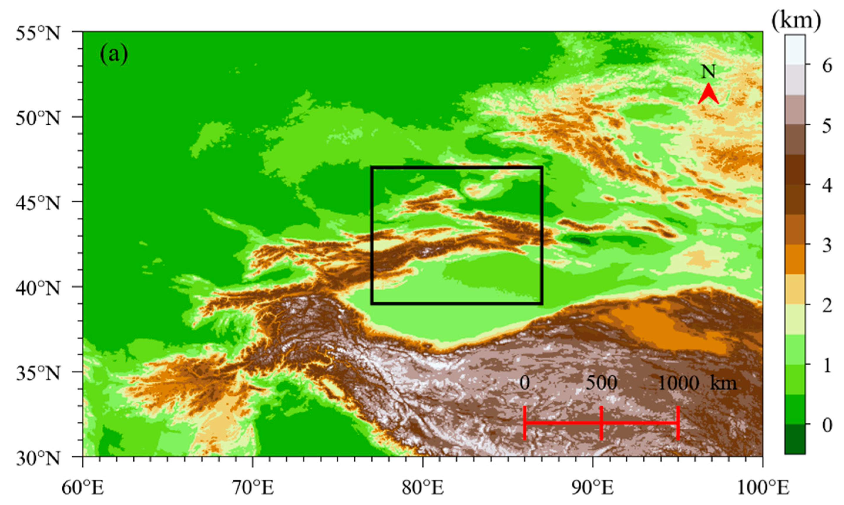
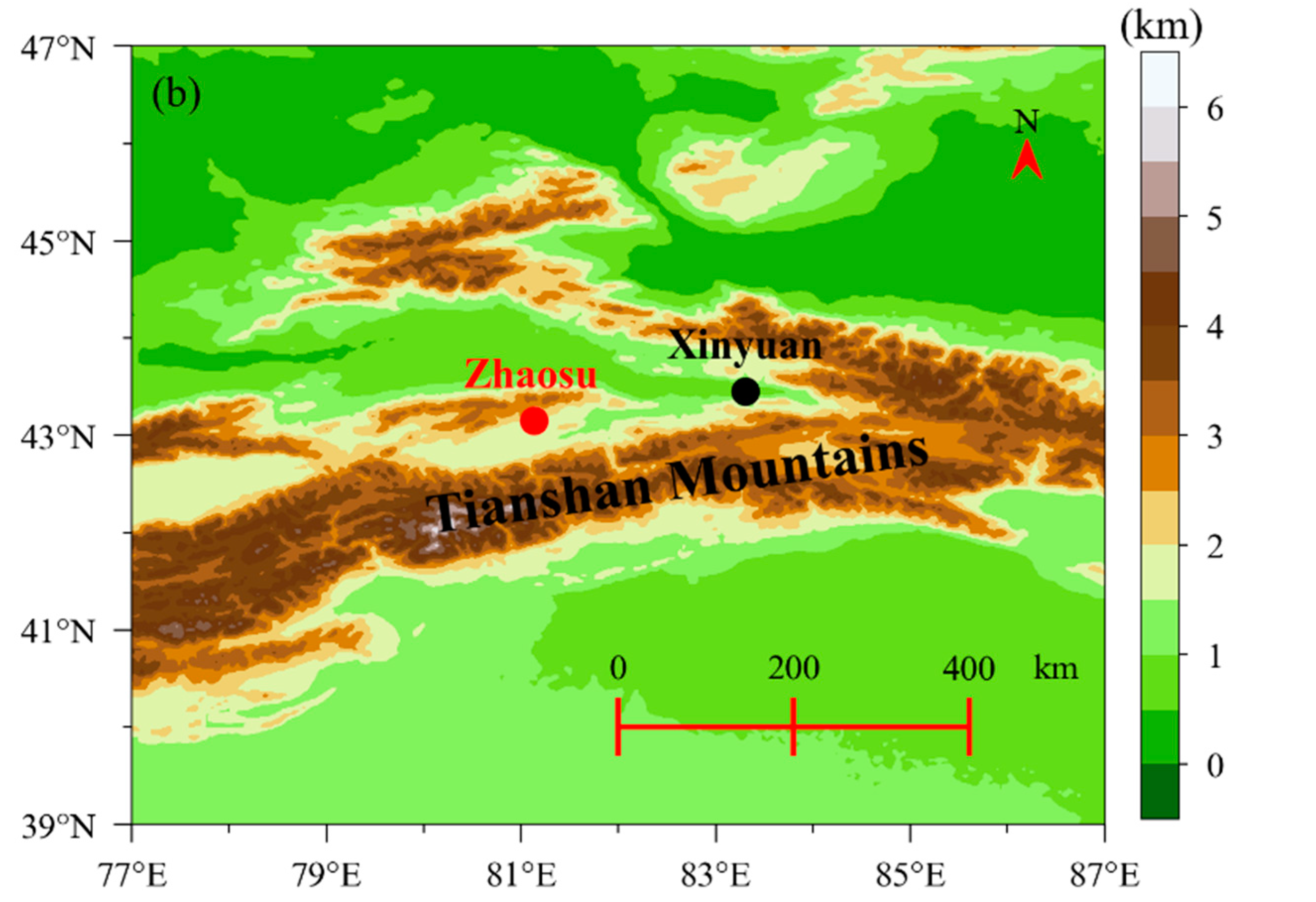
2.1. Study Area and Dataset

The Tianshan Mountains are located in the north of the Qinghai–Tibet Plateau, with the main body located in central Xinjiang, China (Figure 1a). Within this region, Zhaosu (1851 m a.s.l.; 43.14°N, 81.13°E) was the focus area for this study (Figure 1b); the DSD dataset for Zhaosu from 2020 to 2022 was collected based on a second-generation OTT Particle Size Velocity (PARSIVEL²) disdrometer manufactured by OTT Hydromet (Kempten, Germany) [59]. The observation area of Zeng et al. [55] was Xinyuan (928 m a.s.l.; 43.45°N, 83.25°E); they also used a PARSIVEL² disdrometer, and its location is also displayed in Figure 1b. DSD information was obtained by simultaneously recording the particle sizes and fall speeds within a resolution of 1 min [63,64]. More and more studies have used PARSIVEL² disdrometers to conduct research on DSD because of their excellent performance [9,43,44,49,53,54,55,56,57,58,59,60,65,66,67,68]. However, as the high altitude of Zhaosu results in no rainfall in this region during winter [59], this study only considered data from the spring, summer, and fall.

2.2. Quality Control of DSD Data

The quality of the DSD data is affected by many factors, so the quality control processing of the DSD data is crucial. The most critical influencing factors that cannot be ignored are as follows: low signal-to-noise ratio [12,69], low rain rate or number of raindrops during the sampling time [70], and splashing effects or strong winds [64,71]. Therefore, eliminating the impact of these three aspects is important to obtain more accurate DSD data. Previous studies of DSD over the Tianshan Mountains have implemented strict quality control [55,56,57,58,59]. After data quality control, 15,318, 20,785, and 5151 DSD samples were used in the Tianshan Mountains from the spring to fall in Zhaosu, respectively [59].

2.3. RKEE

Rainfall kinetic energy is usually expressed as KE_time (i.e., rainfall kinetic energy flux, J m⁻² h⁻¹) and KE_mm (i.e., rainfall kinetic energy content, J m⁻² mm⁻¹) [4,9,35,36,72,73], which can be calculated using Equations (1) and (2), respectively:

$$K{E}_{time}=\left({\displaystyle \frac{\pi }{12}}\right)\times \left({\displaystyle \frac{1}{{10}^6}}\right)\times \left({\displaystyle \frac{3600}{\mathsf{\Delta }t}}\right)\times \left({\displaystyle \frac{1}{A_{eff}\left(D_i\right)}}\right){\displaystyle \sum }_{i=1}^{32}{n}_i\times {D_i}^3\times {(V\left(D_i\right))}^2$$

(1)

$$K{E}_{mm}={\displaystyle \frac{K{E}_{time}}{R}}$$

(2)

where Δt (s) is the sampling time (60 s); D_i (mm) represents the raindrop diameter; V(D_i) [m s⁻¹] is the raindrop velocity; and A_eff (D_i) [m²] and R (mm h⁻¹) are the effective sampling area [63,74,75] and rain rate, respectively, which can be calculated using Equations (3) and (4):

$$A_{eff}\left(D_i\right)={10}^{-6}\times 180\times \left(30-{\displaystyle \frac{D_i}{2}}\right)$$

(3)

$$R={\displaystyle \frac{6\pi }{{10}^4}}\times {\displaystyle \sum }_{i=1}^{32}N\left(D_i\right)\times {D_i}^3\times V\left(D_i\right)\times \mathsf{\Delta }{D}_i$$

(4)

where ΔD_i (mm) represents the diameter interval and N(D_i) [m⁻³ mm⁻¹] represents DSD, which can be calculated using Equation (5):

$$N\left(D_i\right)={\displaystyle \sum }_{j=1}^{32}{\displaystyle \frac{n_{ij}}{A_{eff}\left(D_i\right)\times \mathsf{\Delta }t\times V\left(D_i\right)\times \mathsf{\Delta }{D}_i}}$$

(5)

where n_ij is the number of drops.

The DSD-based RKEE schemes, including KE_time(R) and KE_mm(D_m) [5,6,7,9,35,55,56,57], are as follows:

$$K{E}_{time }\left(R\right)=a\times R^b$$

(6)

$$K{E}_{mm}\left(D_m\right)=c\times D_m^2+d\times D_m+e$$

(7)

where a, b, c, d, and e are the corresponding coefficients of the RKEE schemes and D_m (mm) is the mass-weighted mean diameter [76], as follows:

$$D_m={\displaystyle \frac{{{\displaystyle \sum }}_{i=1}^{32}N\left(D_i\right)\times D_i^4\times \Delta D_i}{{{\displaystyle \sum }}_{i=1}^{32}N\left(D_i\right)\times D_i^3\times \Delta D_i}}$$

(8)

2.4. QPE for Dual-Polarization Radar

The DSD-based dual-polarization radar QPE algorithms are particularly valuable in enhancing the QPE capability [13,26,27,29,30,31,56,60]. These algorithms are constructed using the variables of the dual-polarization radar, including (1) Z_h/v (i.e., radar reflectivity at horizontal or vertical polarization, mm⁶ m⁻³), (2) Z_dr (i.e., differential reflectivity, dB), and (3) K_dp (i.e., specific differential phase, ° km⁻¹), which can be derived based on the T-matrix scattering method [47,77,78,79] as follows:

$$Z_{h/v}=\left({\displaystyle \frac{4\times {\lambda }^4}{{\pi }^4\times {\left|K_w\right|}^2}}\right)\times {{\displaystyle \int }}_{D_{min}}^{D_{max}}{\left|f_{hh/vv}\left(D\right)\right|}^2\times N\left(D\right)\times dD$$

(9)

$$Z_{dr}=10\times {\log }_{10}\left({\displaystyle \frac{Z_h}{Z_v}}\right)$$

(10)

$$K_{dp}={10}^{-3}\times {\displaystyle \frac{180}{\pi }}\times \lambda \times Re\left\{{{\displaystyle \int }}_{Dmin}^{D_{max}}\left[f_h\left(D\right)-f_v\left(D\right)\right]\times N\left(D\right)\times dD\right\}$$

(11)

where D_max is 8 mm, according to the DSD data in this study; K_w (−) and λ (mm) are the dielectric constant of water (0.9639) and the dual-polarization radar wavelength (33.3 mm for the X-band in this study), respectively; and f_h/v(D) and f_hh/vv(D) represent the forward scattering and backscattering amplitudes of a raindrop, respectively. In this study, the axis–ratio relation reported by Brandes [47] constrained the raindrops.

The DSD-based dual-polarization radar QPE algorithms, including (1) R(Z_h), (2) R(K_dp), (3) R(Z_h,Z_dr), and (4) R(K_dp,Z_dr), are as follows:

$$R\left(Z_h\right)=f\times Z_h^g$$

(12)

$$R\left(K_{dp}\right)=h\times K_{dp}^i$$

(13)

$$R\left(Z_h,Z_{dr}\right)=j\times Z_h^k\times {10}^{l\times Z_{dr}}$$

(14)

$$R\left(K_{dp},Z_{dr}\right)=m\times K_{dp}^n\times {10}^{o\times Z_{dr}}$$

(15)

where f, g, h, i, j, k, l, m, n, and o are the coefficients of the corresponding dual-polarization radar QPE algorithms.

2.5. Assessing RKEE Scheme and Dual-Polarization Radar QPE Algorithm Accuracy

The values of KE_time, KE_mm, and R calculated using Equations (1), (2), and (4) were used to assess the accuracy of the RKEE schemes (Equations (6) and (7)) and the dual-polarization radar QPE algorithms (Equations (12)–(15)). The correlation coefficient (CC), normalized mean absolute error (NMAE), and root mean square error (RMSE) were used to assess the estimators:

$$\mathrm{CC}={\displaystyle \frac{{{\displaystyle \sum }}_{i=1}^n\left(M_i-\overline{M}\right)\times \left(M_{e,i}-\overline{M_e}\right)}{\sqrt{{{\displaystyle \sum }}_{i=1}^n{\left(M_i-\overline{M}\right)}^2}\times \sqrt{{{\displaystyle \sum }}_{i=1}^n{\left(M_{e,i}-\overline{M_e}\right)}^2}}}$$

(16)

$$\mathrm{NMAE}={\displaystyle \frac{\frac{1}{n}\times {{\displaystyle \sum }}_{i=1}^n\left|M_{e,i}-M_i\right|}{\overline{M}}}$$

(17)

$$\mathrm{RMSE}=\sqrt{{\displaystyle \frac{1}{n}}\times {{\displaystyle \sum }}_{i=1}^n{\left(M_{e,i}-M_i\right)}^2}$$

(18)

where $M_i$ and $\overline{M}$ represent the individual and average KE_time, KE_mm, and R calculated from the DSD data, respectively; and $M_{e,i}$ and $\overline{M_e}$ are the individual and average KE_time, KE_mm, and R derived from the RKEE schemes and dual-polarization radar QPE algorithms, respectively.

2.6. Classification of Rainfall Types

Stratiform and convective rainfall are the two basic rainfall types, and many researchers have proposed classification methods for these rainfall types [12,17,18,62,76,80]. Here, we used two classic classification methods of rainfall types to divide DSD data into stratiform and convective rainfall. Specifically, the first classification method was reported by Bringi et al. [62], based on the log₁₀N_w (normalized intercept parameter)–D₀ (median volume diameter) space (BR09) [36,59,62,81,82]. The second classification scheme was reported by Bringi et al. [18], considering R and the standard deviation of R (BR03) [18,19,20,21,22,23,24,25]. The simultaneous application of these two classification schemes (BR09 and BR03) was based on their widespread recognition and the characteristics of rainfall in arid regions. BR09 and BR03 are both classic classification schemes for rainfall types, which have been applied in many regions, especially the BR03 classification. More importantly, the Tianshan Mountains are located in arid areas with insufficient water vapor supply, and the convective rainfall in this region has the characteristics of a short duration, a high variability, and a relatively low R compared to monsoon areas [50,51,52]. BR03 can be specifically expressed when there is at least 10 consecutive 1 min rainfall samples; the rainfall is determined to be stratiform rainfall (convective rainfall) if R is >0.5 (5) mm h⁻¹ and the standard deviation of R is < (>) 1.5 mm h⁻¹. In previous studies based on the BR03, we found that even in summer, there were fewer convective rainfall samples in the Tianshan Mountains [53,54,56,58], which were affected by the short duration, high variability, and low R of convective rainfall in the region. Based on this, the widely recognized BR09 has also been applied in this study. Specifically, BR09 can be expressed as samples located below (above) the equation log₁₀N_w = −1.6D₀ + 6.3 in the log₁₀N_w − D₀ space that are classified as stratiform rainfall (convective rainfall). It should be noted that we recognize both of these two classic classification methods, and there is no superiority or inferiority between BR09 and BR03; only the classification principles are different. Furthermore, the simultaneous application of BR09 and BR03 provided convenience for comparing different classification schemes of rainfall types in this study and comparing them with previous studies based only on one classification scheme of rainfall type in other regions. After the classification of rainfall types for all DSD samples, the number of DSD samples for stratiform rainfall (convective rainfall) classified by BR09 was 40,380 (871), while the number classified by BR03 was 10,349 (228). In terms of seasons, for stratiform rainfall under BR09 (BR09_S), the numbers of the samples were 15,115, 20,148, and 5117 from spring to fall, respectively, whereas for convective rainfall under BR09 (BR09_C), the numbers of the samples were 202, 636, and 33 from spring to fall, respectively. For stratiform rainfall under BR03 (BR03_S), the numbers of the samples were 4523, 4734, and 1092 from spring to fall, respectively, while for convective rainfall under BR03 (BR03_C), the numbers of the samples were 119 and 109 in spring and summer, respectively. Notably, there were no samples of convective rainfall in the fall under BR03. For a more detailed explanation of the DSD data and the process of classifying rainfall types in this study, please refer to Zeng et al. [59].

3. Results

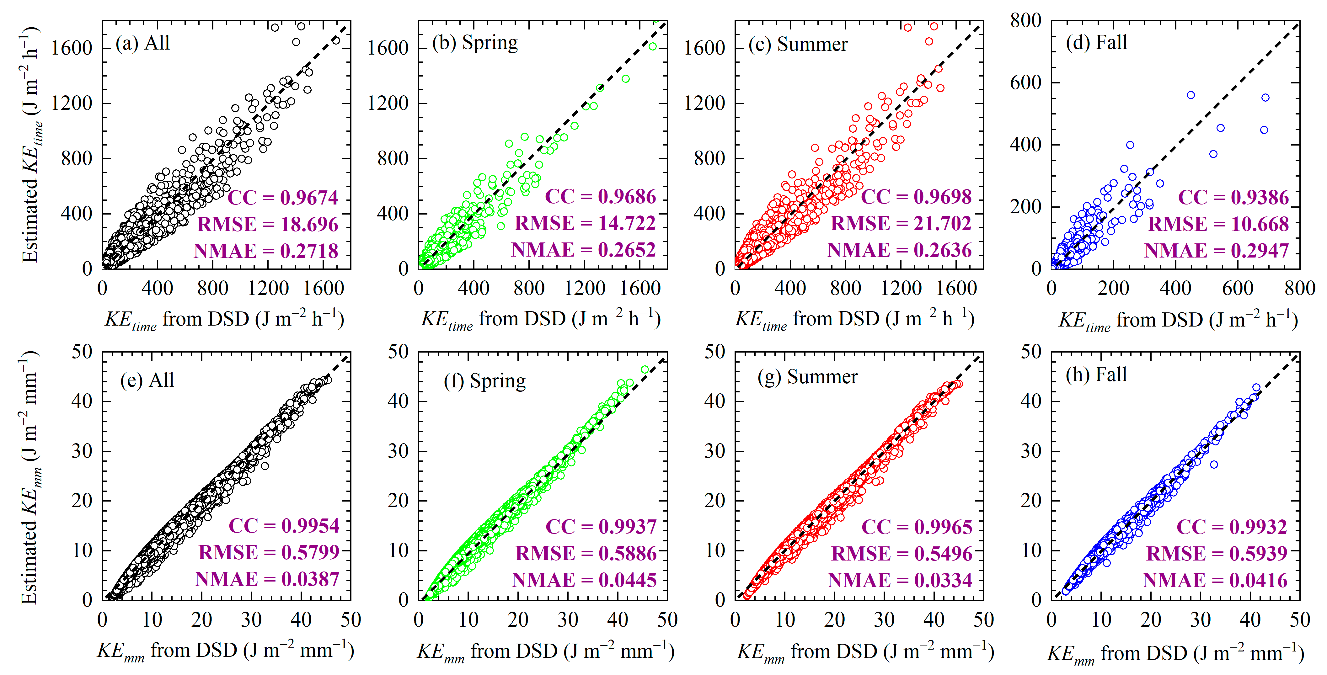
3.1. Seasonal RKEE Variation

As “the water tower of central Asia”, heavy rainfall in the Tianshan Mountains often causes landslides, mudslides, and floods, owing to the steep terrain; the degree of damage caused by these secondary disasters can be estimated to some extent by rainfall kinetic energy (KE), including KE_time and KE_mm [57,83]. Obtaining the rainfall KE from DSD information overcomes the limitations of expensive direct measurement instruments and is an important method for obtaining rainfall KE [4]. Figure 2 shows seasonal variations in KE_time and KE_mm. For the entire data and spring, the peak distribution of KE_time was 4.5 J m⁻² h⁻¹; for summer and fall, KE_time was mostly distributed around 6.5 and 3.0 J m⁻² h⁻¹, respectively; mean KE_time (purple solid line) was the largest (smallest) at 29.418 (14.006) J m⁻² h⁻¹ in the summer (fall) (Figure 2a). The peak distribution of KE_mm for the entire data and the three seasons was 7.6, 6.8, 8.0, and 8.2 J m⁻² mm⁻¹, respectively, and mean KE_mm (purple solid line) was largest (smallest) at 12.307 (9.826) J m⁻² mm⁻¹ in summer (spring) (Figure 2b).

The scatterplots of KE_time vs. R for the entire dataset and the KE_time–R relationship across the seasons are shown in Figure 3. For ease of comparison, previous results from Zeng et al. [55], Seela et al. [83], and Wu et al. [36] are also shown. For the entire dataset, the KE_time–R relation was KE_time = 12.495R^1.285. The fitting curves for summer and fall were similar to those for the entire dataset. For the same R, KE_time was slightly smaller in spring or fall than in summer. Compared with Zeng et al. [55], regardless of the entire dataset or different seasons, given the R value, the KE_time of Zhaosu was almost always greater than that of Xinyuan. The KE_time–R relationship for the entire data at Enshi (a southwestern mountain area of China), as reported by Wu et al. [36], was higher than that for the entire data at Zhaosu when R < 35.0 mm h⁻¹, and vice versa when R > 35.0 mm h⁻¹. Compared with all the above results, for the same R, Seela et al. [83] reported the smallest KE_time for typhoons in Palau, an island in the Western Pacific. The variation among each curve in Figure 3 was relevant to their own elevation or climate conditions.

For RKEE, the KE_mm–D_m relationship is also an important RKEE scheme. Figure 4 shows scatterplots of KE_mm vs. D_m for the entire dataset and for different seasons at Zhaosu compared with those for previous results [55,83]. For the entire dataset, the KE_mm–D_m relationship was KE_mm = −2.260D_m² + 21.953D_m − 8.899. The fitting curves across the seasons were very close to those for the entire dataset until D_m was >3.6 mm. When D_m > 3.2 mm, as D_m increased, the difference between KE_mm in summer and that in spring and fall gradually increased. However, the seasonal variation in KE_mm was not as significant as that at Xinyuan [55]. Another difference between Zhaosu and Xinyuan was that, for a given D_m value, a larger KE_mm was observed in Zhaosu than in Xinyuan, whereas the opposite was true for D_m > 2.8 mm in fall. Compared with all the above results, for 0.6 mm < D_m < 3.8 mm, Seela et al. [83] reported the smallest KE_mm of KE_mm–D_m relationship for a typhoon in Palau, Western Pacific.

To evaluate the accuracy of the derived RKEE schemes, we compared the estimated rainfall KE for different RKEE schemes, as shown in Figure 3 and Figure 4, with the rainfall KE directly derived from DSD based on Equations (1) and (2). Figure 5 shows scatterplots of KE_time and KE_mm computed from the derived RKEE schemes and DSD in terms of the CC, RMSE, and NMAE. The performances of the RKEE schemes of KE_mm were superior to those of KE_time for all seasons and the entire dataset, and were characterized by more clustered scatterers along the 1:1 line and larger CC (>0.99). For the RKEE schemes of KE_mm across seasons, the performance of KE_mm in summer was superior to that in spring and fall, with a larger CC (0.9965) and smaller RMSE (0.5496 J m⁻² mm⁻¹) and NMAE (0.0334 J m⁻² mm⁻¹). Similarly, the performance of KE_time in summer was superior to that in spring and fall, with a larger CC (0.9698) and smaller NMAE (0.2636 J m⁻² h⁻¹), while a larger RMSE in summer was mainly caused by the larger KE_time, as shown in Figure 2a. This may be related to the fact that summer has more samples compared to other seasons. Overall, the RKEE schemes performed well for both the entire dataset and the different seasons.

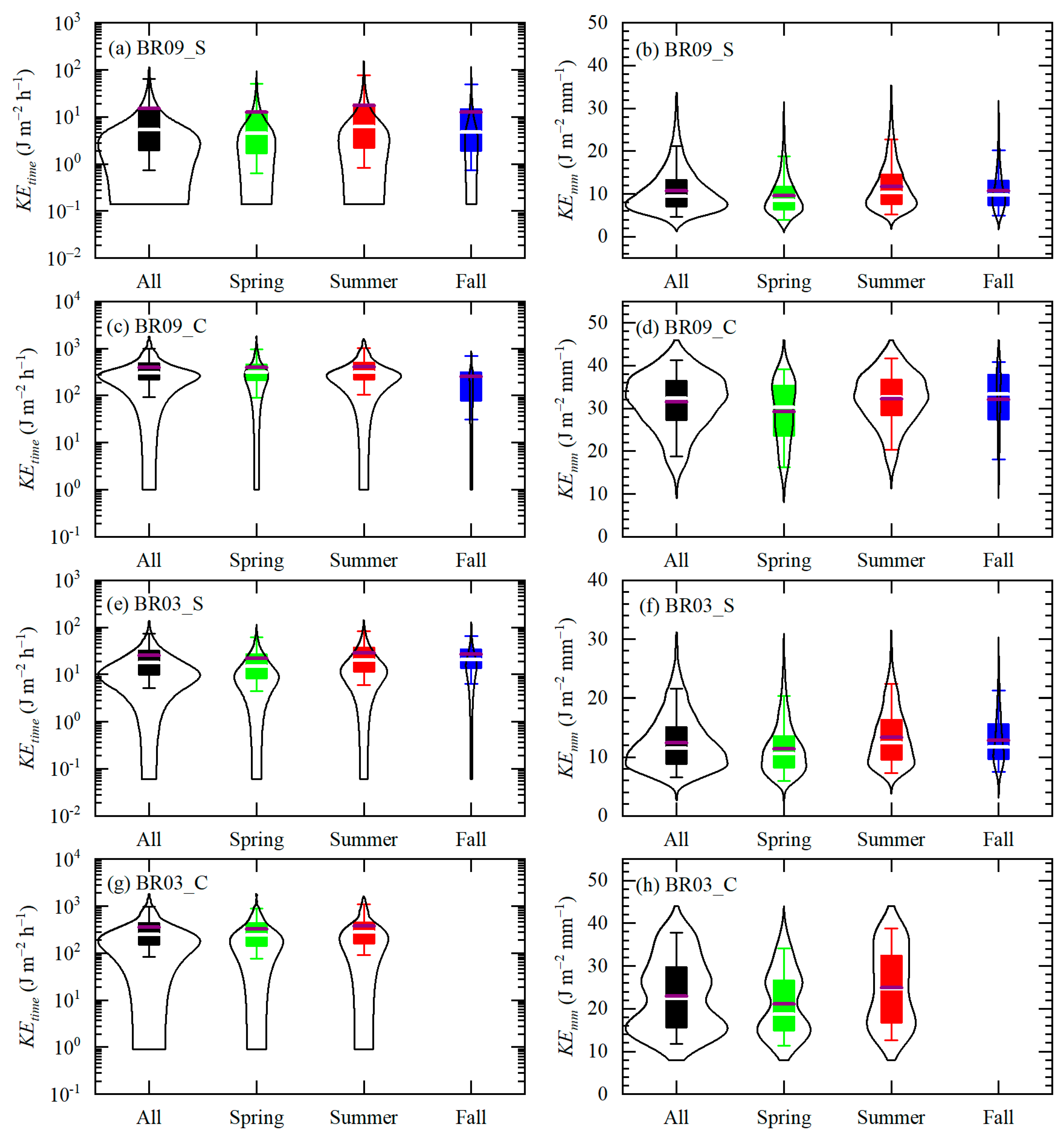
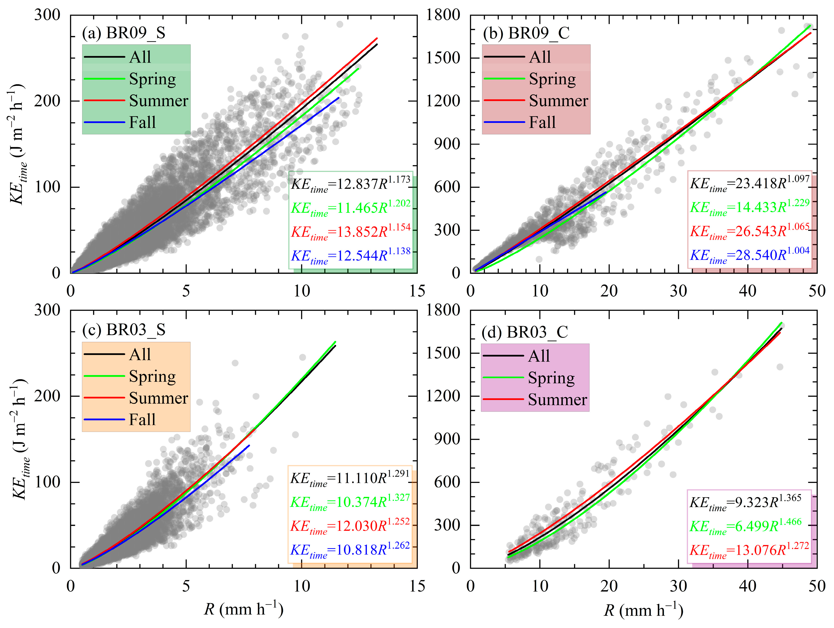
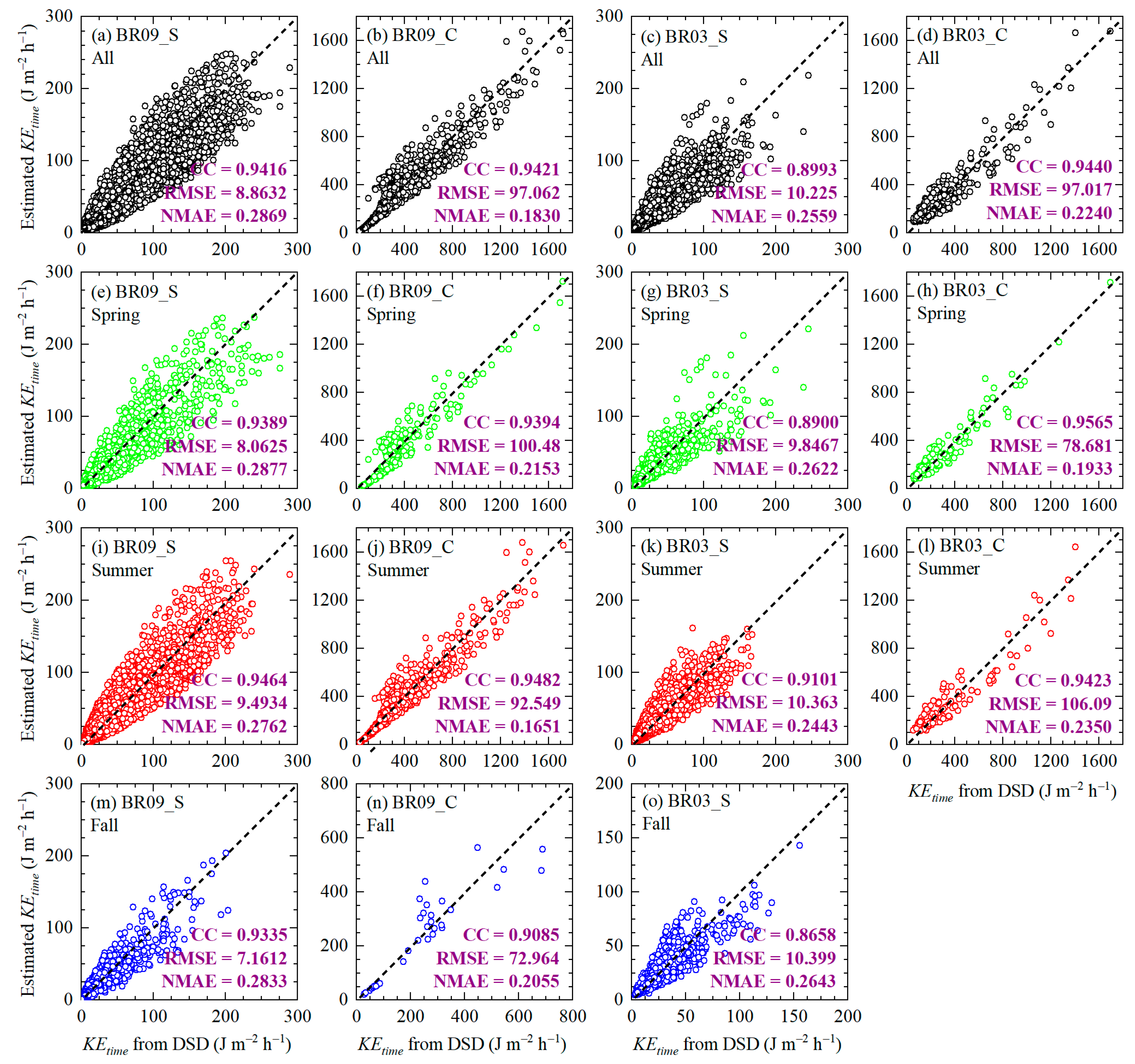
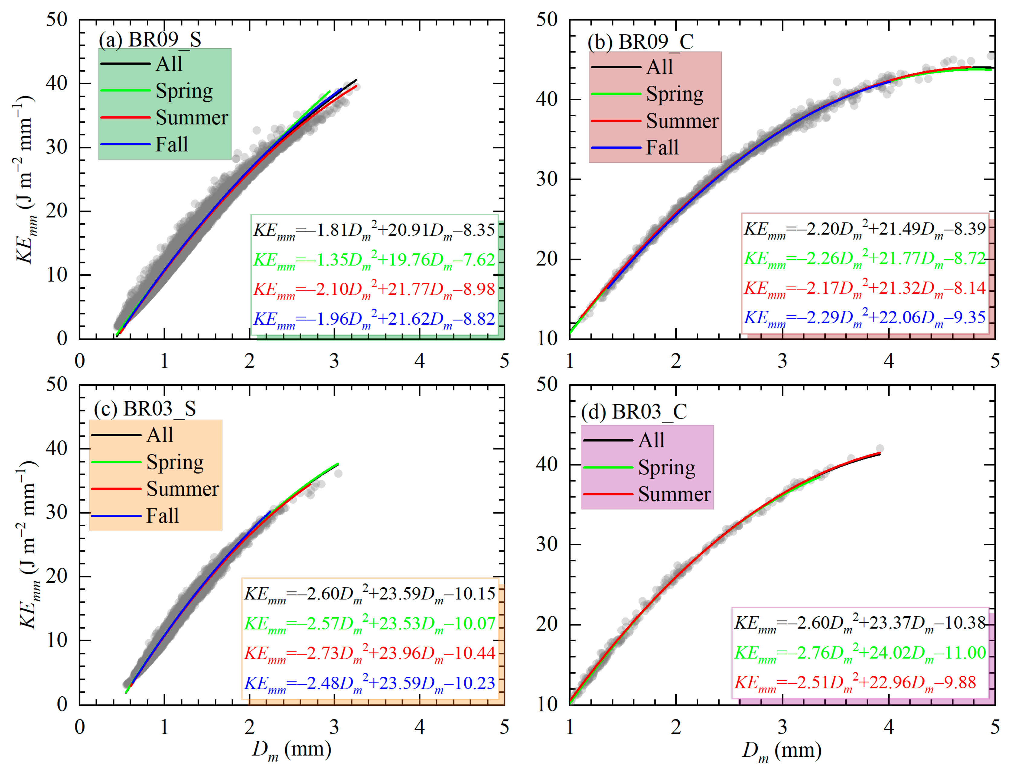
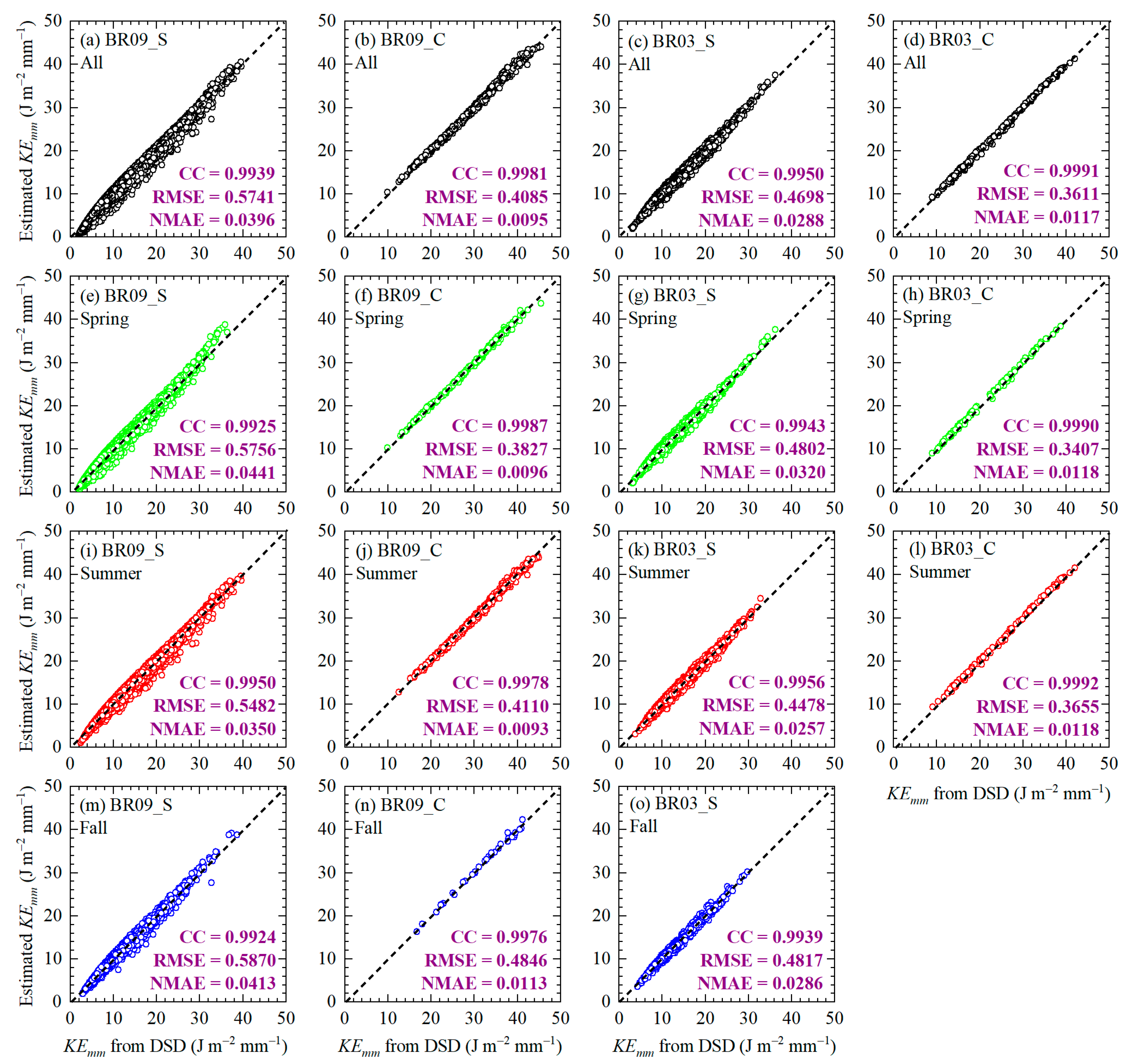
3.2. Seasonal RKEE Variation for Different Rainfall Types

Stratiform and convective rainfall are two basic types of rainfall with significant differences in their microphysical characteristics [17,18,19,20,21,22,23,24,25,62,80,81,82]. Therefore, it is necessary to explore the RKEE for different rainfall types. Figure 6 shows the seasonal variations in the distributions of KE_time and KE_mm for stratiform and convective rainfall under BR09 and BR03 at Zhaosu. For stratiform rainfall under BR09 (BR09_S), the peak distribution of KE_time was 5.0 J m⁻² h⁻¹, with a mean KE_time (purple solid line) at its largest (smallest) at 17.535 (12.489) J m⁻² h⁻¹ in the summer (spring) (Figure 6a). For convective rainfall under BR09 (BR09_C), the KE_time with the highest distribution across the different seasons was ~260.0 J m⁻² h⁻¹, and the mean KE_time was largest (smallest) at 405.907 (249.190) J m⁻² h⁻¹ in summer (fall) (Figure 6c). Meanwhile, for stratiform rainfall under BR03 (BR03_S), the mean KE_time was largest (smallest) at 28.590 (21.558) J m⁻² h⁻¹ in summer (spring) (Figure 6e); for convective rainfall under BR03 (BR03_C), the mean KE_time was 379.887 (325.083) J m⁻² h⁻¹ in summer (spring) (Figure 6g). Furthermore, for BR09_S (BR09_C), the mean KE_mm (purple solid line) was largest at 11.677 (32.209) J m⁻² mm⁻¹ in summer and smallest at 9.566 (29.265) J m⁻² mm⁻¹ in spring (Figure 6b,d). For BR03_S (BR03_C), the mean KE_mm was largest at 13.342 (24.920) J m⁻² mm⁻¹ in summer, and smallest at 11.425 (21.172) J m⁻² mm⁻¹ in spring (Figure 6f,h). In all seasons, for both stratiform and convective rainfall under both BR03 and BR09, summer hadthe largest mean KE_time and KE_mm.

The scatterplots of KE_time vs. R for the entire dataset, and the KE_time–R relationship for stratiform and convective rainfall across the seasons under BR09 and BR03 at Zhaosu, are shown in Figure 7. Under BR09_S, the KE_time–R relation was revealed as KE_time = 12.837R^1.173 for the entire dataset. In terms of seasons, for the same R, KE_time was slightly smaller in spring or fall than that in summer, and KE_time was slightly larger in spring than that in fall when R > 4.0 mm h⁻¹ (Figure 7a). Under BR09_C, the KE_time–R relation was KE_time = 23.418R^1.097 for the entire dataset, and the KE_time–R relationships were KE_time = 14.433R^1.229, KE_time = 26.543R^1.065, and KE_time = 28.540R^1.004 for spring, summer, and fall, respectively (Figure 7b). Meanwhile, under BR03_S, the KE_time–R relationship was KE_time = 11.110R^1.291 for the entire dataset, and the KE_time–R relationships were KE_time = 10.374R^1.327, KE_time = 12.030R^1.252, and KE_time = 10.818R^1.262 for spring, summer, and fall, respectively (Figure 7c). Under BR03_C, for the same R, KE_time was slightly larger in spring than that in summer for R > 37.0 mm h⁻¹, and vice versa when R < 37.0 mm h⁻¹ (Figure 7d). In summary, the RKEE schemes based on the KE_time–R relationships are largely constrained by different classification methods, rainfall types, and seasons.

To further evaluate the accuracy of the derived RKEE schemes across seasons under BR09 and BR03, we compared the KE_time estimated by various RKEE schemes with the KE_time directly derived from the DSD based on Equation (1). Figure 8 shows the scatterplots of KE_time computed from the derived RKEE schemes and KE_time computed from DSD with CC, RMSE, and NMAE across seasons under BR09 and BR03. Under BR09_S and BR09_C, the values of CC for the entire dataset and all seasons were >0.93, except for those in fall under BR09_C (0.9085), whereas under BR03_S, the values of CC for the entire dataset and all seasons were <0.90, except for those in summer (0.9101). Furthermore, the performance of the RKEE schemes of KE_time for the entire data and all seasons under BR03_C was superior to those under BR03_S, characterized by a larger CC (>0.94) and a smaller NMAE (<0.24 J m⁻² h⁻¹); the larger RMSE under BR03_C was mainly caused by the larger KE_time across seasons, as shown in Figure 6g. More importantly, from a seasonal perspective, under BR09_S, BR09_C, and BR03_S, the performance of KE_time in summer was superior to that in other seasons, characterized by a larger CC and a smaller NMAE, while under BR03_C, the performance of KE_time in spring was superior to that in summer.

Scatterplots of KE_mm vs. D_m for the entire dataset and seasonal variation in the KE_mm–D_m relationship for different rainfall types under BR09 and BR03 are shown in Figure 9. Under BR09_S, for the entire data, the KE_mm–D_m relationship was KE_mm = −1.81D_m² + 20.91D_m − 8.35. In terms of seasons, when D_m > 2.2 mm, KE_mm was slightly larger in spring than that in summer and fall (Figure 9a). Under BR09_C, for the entire dataset, the KE_mm–D_m relationship was KE_mm = −2.20D_m² + 21.49D_m − 8.39, and the seasonal variation in the KE_mm–D_m relationship was insignificant compared to that under BR09_S (Figure 9b). Meanwhile, under BR03_S, the KE_mm–D_m relationship was KE_mm = −2.60D_m² + 23.59D_m − 10.15 for the entire data, and the KE_mm–D_m relationships across the seasons were KE_mm = −2.57D_m² + 23.53D_m − 10.07, KE_mm = −2.73D_m² + 23.96D_m − 10.44, and KE_mm = −2.48D_m² + 23.59D_m − 10.23, respectively (Figure 9c). Under BR03_C, the KE_mm–D_m relationship was KE_mm = −2.60D_m² + 23.37D_m − 10.38 for the entire dataset, and the KE_mm–D_m relationship across the seasons was insignificant compared to that under BR03_S (Figure 9d). In summary, RKEE schemes based on KE_mm–D_m relationships were largely constrained by different rainfall types and their classification methods. In addition, the KE_mm–D_m relationship across the seasons during stratiform rainfall was more pronounced than that during convective rainfall.

To further evaluate the accuracy of the derived RKEE schemes across seasons in BR09 and BR03, we compared the estimated KE_mm using various RKEE schemes with the KE_mm directly derived from the DSD based on Equation (2). Figure 10 shows the scatterplots of KE_mm computed from the derived RKEE schemes and KE_mm computed from DSD with CC, RMSE, and NMAE for the different rainfall types under BR09 and BR03. All RKEE schemes listed in Figure 10 had excellent performance, characterized by large a CC (>0.99) and a small NMAE (<0.05 J m⁻² mm⁻¹) and RMSE (<0.60 J m⁻² mm⁻¹), but there were also some differences between these RKEE schemes. Specifically, the performance of the RKEE schemes of KE_mm for all data and seasons under BR09_C (BR03_C) was superior to that under BR09_S (BR03_S), which was characterized by more clustered scatterers along the 1:1 line, a larger CC, and smaller a NMAE and RMSE. In addition, under BR09_S and BR03_S, the performance of the RKEE schemes of KE_mm in summer was superior to that in other seasons, with a larger CC and smaller NMAE and RMSE.

Overall, for both the entire sample and samples of different rainfall types, obtaining KE_mm based on D_m (KE_mm–D_m relation) was more accurate than obtaining KE_time based on R (KE_time–R relation). However, it was worth noting that R is easier to obtain than D_m, as the former can be obtained through various methods including observations from widely distributed meteorological stations. In addition, many reanalysis datasets and satellite products also included R. Therefore, obtaining KE_time through the KE_time–R relation was easier and more convenient, and had a broader application space in the future.

3.3. Seasonal Variation of Dual-Polarization Radar QPE

Previous studies have revealed that using the method of T-matrix scattering with DSD information to obtain the dual-polarization radar variables Z_h, Z_dr, and K_dp according to Equations (9)–(11) is reliable and accurate [13,26,27,29,30,31,32,56,60]. Figure 11 shows the seasonal variations in the distributions of dual-polarization radar variables Z_h, Z_dr, and K_dp at Zhaosu. For the entire data and three seasons (spring, summer, fall), the peak distribution of Z_h was ~19.0 dBZ, with mean values (gray solid line) close to ~21.6, ~20.4, ~22.7, and ~20.9 dBZ, respectively (Figure 11a). Z_dr’s highest distributions for the entire dataset and three seasons were 0.11, 0.09, 0.13, and 0.13 dB, respectively, and the mean value of Z_dr (gray solid line) was largest in summer (0.388 dB) and smallest in spring (0.269 dB) (Figure 11b). For fall, K_dp was mostly distributed around 0.007 ° km⁻¹, while for other seasons, the peak distribution of K_dp was 0.011 ° km⁻¹; the mean K_dp (gray solid line) was the smallest (largest) in fall (summer) at 0.029 (0.070) ° km⁻¹ (Figure 11c).

The dual-polarization radar QPE algorithms (single-parameter algorithms R(Z_h) and R(K_dp), and double-parameter algorithms R(Z_h,Z_dr) and R(K_dp,Z_dr)) across the seasons are listed in

Table 1. Seasonal variation in DSD-based QPE algorithms of dual-polarization radar at Zhaosu.

	R(Zh) = f × Zhg		R(Kdp) = h × Kdpi		R(Zh,Zdr) = j × Zhk × 10l×Zdr			R(Kdp,Zdr) = m × Kdpn × 10o×Zdr
	f	g	h	i	j	k	l	m	n	o
All	0.067	0.504	13.481	0.669	0.018	0.766	−0.345	25.670	0.822	−0.170
Spring	0.067	0.516	14.655	0.666	0.018	0.800	−0.446	30.275	0.827	−0.218
Summer	0.064	0.506	13.097	0.680	0.016	0.763	−0.311	24.184	0.831	−0.156
Fall	0.072	0.491	13.176	0.649	0.018	0.822	−0.593	30.789	0.816	−0.274

. Discrepancies were observed across the seasons for each of the four types of QPE algorithms. Specifically, the coefficient f (g) of the R(Z_h) algorithm varied from 0.064 (0.491) to 0.072 (0.516) between the seasons. Similarly, for the R(K_dp) algorithm, the coefficient h (i) varied from 13.097 (0.649) to 14.655 (0.680) between the seasons; for the R(Z_h,Z_dr) algorithm, the coefficients j, k, and l varied from 0.016 to 0.018, 0.763 to 0.822, and −0.593 to −0.311 across the seasons, respectively. In addition, for the R(K_dp,Z_dr) algorithm, the coefficient m varied from 24.184 to 30.789, and the variability of coefficient o (−0.156 to −0.274) was relatively greater than that of coefficient n (0.816 to 0.831) across the seasons.

Previous studies have shown that evaluating the performance of various dual-polarization radar QPE algorithms based on DSD is important and necessary. R calculated according to Equation (4) was used to evaluate the DSD-based QPE algorithms of the dual-polarization radar [13,30,31,48,56,60,84]. Figure 12 shows the scatterplots of R estimated according to the QPE algorithms and R calculated according to Equation (4) with CC, RMSE, and NMAE across the seasons. For the entire data and all seasons, double-parameter algorithms performed better than single-parameter algorithms with more clustered scatterers on the 1:1 line, larger CC (>0.96), and smaller RMSE (<0.8 mm h⁻¹) and NMAE (<0.23 mm h⁻¹). Moreover, for single-parameter algorithms, regardless of the entire dataset or season, the performance of the R(K_dp) algorithm was superior to that of the R(Z_h) algorithm. Similarly, for the double-parameter schemes, the R(K_dp, Z_dr) algorithm performed better than the R(Z_h, Z_dr) algorithm. In addition, both single-parameter algorithms performed the worst in fall, the R(Z_h, Z_dr) algorithm performed the worst in summer, and the R(K_dp, Z_dr) algorithm showed little difference in performance across seasons.

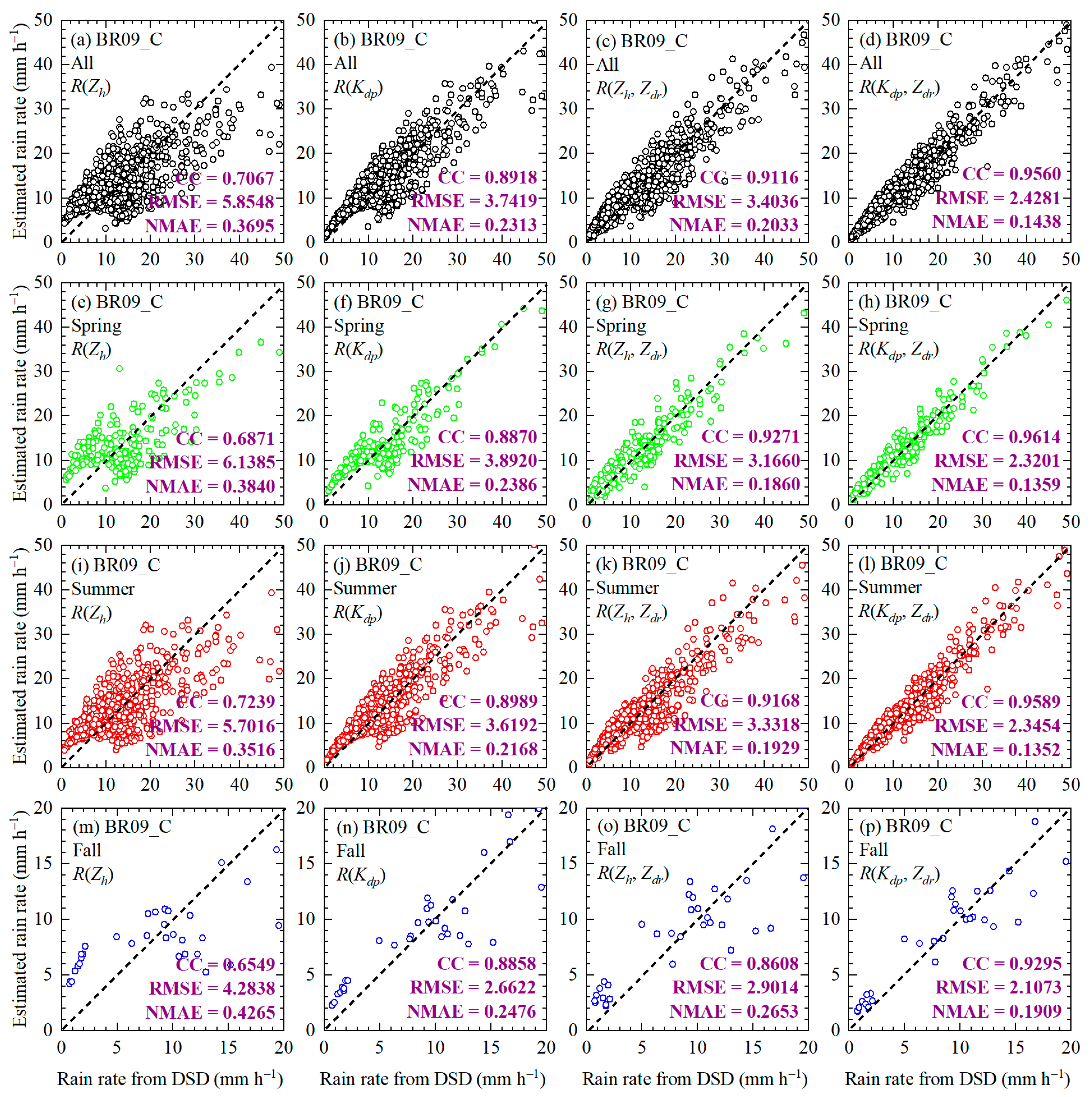
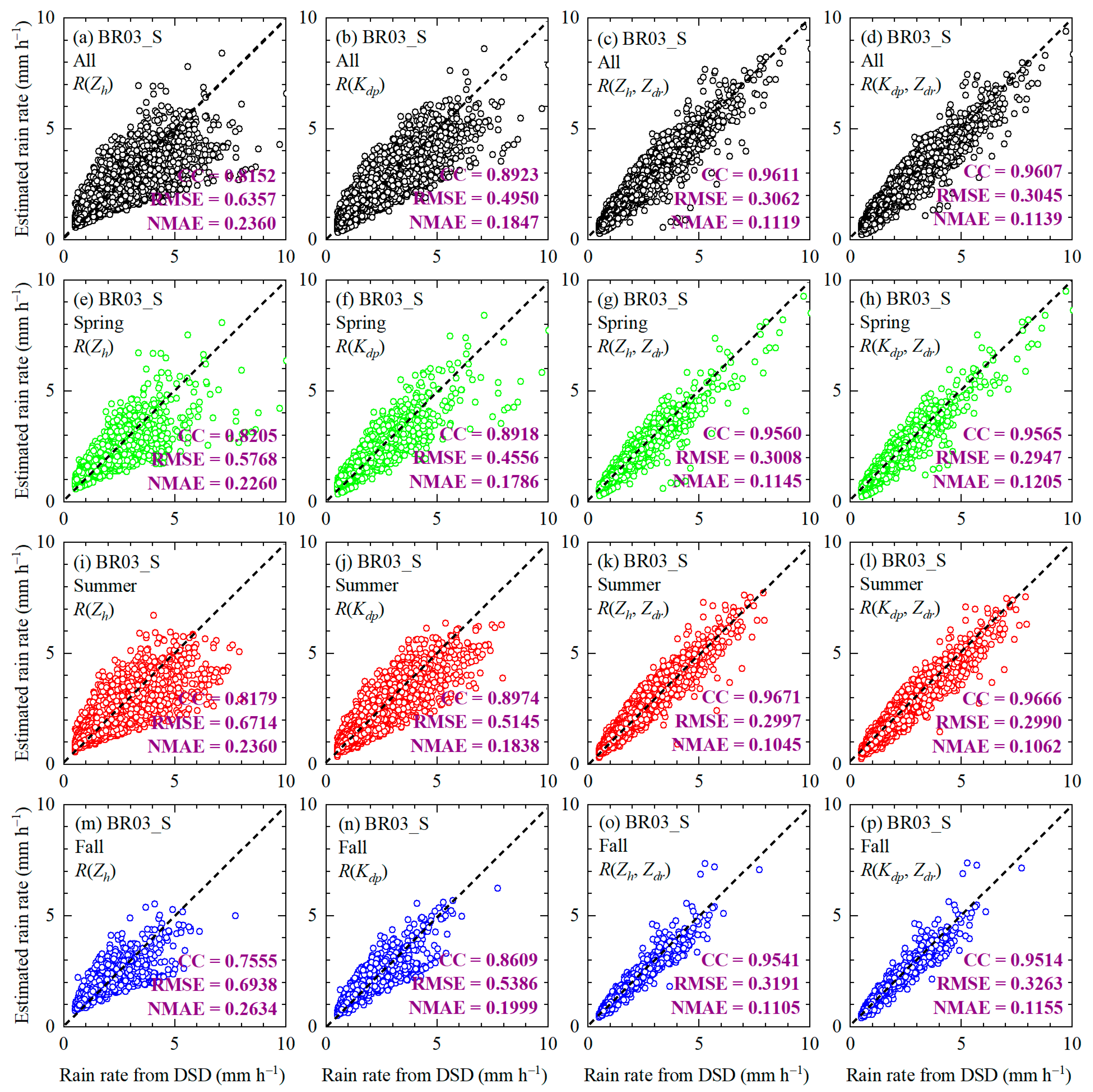
3.4. Seasonal Variation of Dual-Polarization Radar QPE for Different Rainfall Types

Figure 13 shows the seasonal variations in the distributions of the dual-polarization radar variables Z_h, Z_dr, and K_dp for stratiform and convective rainfall under BR09 and BR03 at Zhaosu. For BR09_S, Z_h with the highest distribution across the seasons was ~19.0 dBZ, and the mean Z_h (gray solid line) was largest (smallest) at 22.01 (20.11) J m⁻² h⁻¹ in summer (spring) (Figure 13a). For BR09_C, the peak distribution of Z_h was ~42.5 dBZ, and the mean Z_h was largest at 44.73 dBZ (smallest at 42.05 dBZ) in summer (fall) (Figure 13d). Meanwhile, for BR03_S, the mean Z_h was largest at 27.32 dBZ (smallest at 25.52 dBZ) in summer (spring) (Figure 13g), and for BR03_C, the mean Z_h was 41.96 dBZ (40.23 dBZ) in summer (spring) (Figure 13j). Furthermore, for BR09_S (BR09_C), Z_dr with the highest distribution across the seasons was ~0.1 (1.4) dB and the mean Z_dr (gray solid line) was largest at 0.34 (1.81) dB in summer (fall), and smallest at 0.25 (1.56) dB in spring (Figure 13b,e). For BR03_S (BR03_C), the mean Z_dr was largest at 0.45 (1.22) dB in summer, and the smallest at 0.35 (0.93) dB in spring (Figure 13h,k). In addition, for BR09_S (BR09_C), the peak distribution of K_dp was ~0.006 (0.65) ° km⁻¹, and the mean value of K_dp (gray solid line) was close to ~0.031 (1.085), ~0.025 (1.034), ~0.037 (1.123), and ~0.025 (0.677) ° km⁻¹ for the entire data, spring, summer and fall, respectively (Figure 13c,f). For BR03_S (BR03_C), the mean K_dp was the largest at 0.058 (1.003) ° km⁻¹ in summer and the smallest at 0.042 (0.798) ° km⁻¹ in spring (Figure 13i,l).

The dual-polarization radar QPE algorithms for stratiform and convective rainfall under BR09 across seasons based on the DSD information at Zhaosu are listed in

Table 2. Seasonal variation of the DSD-based QPE algorithms of a dual-polarization radar for different rainfall types under BR09 at Zhaosu.

	R(Zh) = f × Zhg		R(Kdp) = h × Kdpi		R(Zh,Zdr) = j × Zhk × 10l×Zdr			R(Kdp,Zdr) = m × Kdpn × 10o×Zdr
BR09_S	f	g	h	i	j	k	l	m	n	o
All	0.060	0.521	14.640	0.690	0.014	0.867	−0.675	38.775	0.864	−0.370
Spring	0.063	0.524	15.717	0.688	0.015	0.858	−0.653	38.710	0.853	−0.352
Summer	0.056	0.525	14.318	0.699	0.013	0.877	−0.680	38.794	0.876	−0.370
Fall	0.054	0.535	15.828	0.711	0.016	0.852	−0.669	37.766	0.849	−0.372
BR09_C	f	g	h	i	j	k	l	m	n	o
All	0.067	0.504	12.591	0.762	0.009	0.808	−0.291	22.139	0.894	−0.144
Spring	0.097	0.482	14.194	0.703	0.018	0.772	−0.367	26.876	0.849	−0.186
Summer	0.054	0.521	12.098	0.786	0.006	0.837	−0.277	20.926	0.919	−0.135
Fall	0.102	0.451	12.127	0.692	0.048	0.615	−0.225	17.978	0.763	−0.102

. The coefficient f(g) of the R(Z_h) algorithm varied from 0.054 (0.524) to 0.063 (0.535) between different seasons for BR09_S, while the coefficient f (g) of the R(Z_h) algorithm varied from 0.054 (0.451) to 0.102 (0.521) between different seasons for BR09_C. Similarly, for the R(K_dp) algorithm, the coefficient h(i) varied from 14.318 (0.688) to 15.828 (0.711) across seasons for BR09_S, while the coefficient h(i) varied from 12.098 (0.692) to 14.194 (0.786) across seasons for BR09_C. Furthermore, for the R(Z_h,Z_dr) algorithm, the coefficients j, k, and l varied from 0.013 to 0.016, 0.852 to 0.877, and −0.653 to −0.680 across seasons for BR09_S, respectively, while the coefficients j, k, and l varied from 0.006 to 0.048, 0.615 to 0.837, and −0.225 to −0.367 across seasons for BR09_C, respectively. In addition, for the R(K_dp,Z_dr) algorithm, the differences in the coefficients m, n, and o across seasons during convective rainfall were greater than those during stratiform rainfall.

Figure 14 and Figure 15 show scatterplots of estimated R based on QPE algorithms and calculated R according to Equation (4) with respect to CC, RMSE, and NMAE for BR09_S and BR09_C across the seasons. For both stratiform and convective rainfall, and for both the entire data and all seasons, double-parameter algorithms were superior to single-parameter algorithms, with more clustered scatterers along the 1:1 line, a larger CC, and a smaller RMSE and NMAE, except for the R(K_dp, Z_dr) algorithm in the fall under BR09_C. Moreover, the R(K_dp) algorithm was superior to the R(Z_h) algorithm for both BR09_S and BR09_C across seasons. Meanwhile, the performance of the R(Z_h, Z_dr) algorithm was better than that of the R(K_dp, Z_dr) algorithm for BR09_S in spring and fall, whereas the opposite was true for the BR09_C in all seasons. Similarly, seasonal variations in the various QPE algorithms cannot be ignored. For example, for BR09_C, the single-parameter algorithms performed the best (worst) in summer (fall) and the R(Z_h, Z_dr) algorithm performed the best (worst) in spring (fall), whereas for BR09_S, the R(K_dp, Z_dr) algorithm performed the best (worst) in summer (spring).

Similar to Table 2, the dual-polarization radar QPE algorithms for stratiform and convective rainfall under BR03 across seasons based on the DSD information at Zhaosu are listed in

Table 3. Seasonal variation of QPE algorithms of DSD-based dual-polarization radar for different rainfall types under BR03 at Zhaosu.

	R(Zh) = f × Zhg		R(Kdp) = h × Kdpi		R(Zh,Zdr) = j × Zhk × 10l×Zdr			R(Kdp,Zdr) = m × Kdpn × 10o×Zdr
BR03_S	f	g	h	i	j	k	l	m	n	o
All	0.142	0.403	11.178	0.575	0.017	0.842	−0.641	36.243	0.837	−0.345
Spring	0.154	0.391	10.830	0.558	0.017	0.835	−0.622	35.616	0.829	−0.329
Summer	0.126	0.418	11.580	0.597	0.015	0.859	−0.655	37.503	0.855	−0.353
Fall	0.158	0.394	11.653	0.577	0.019	0.824	−0.644	35.790	0.820	−0.357
BR03_C	f	g	h	i	j	k	l	m	n	o
All	0.526	0.335	15.942	0.539	0.046	0.662	−0.281	25.984	0.776	−0.155
Spring	0.506	0.346	16.909	0.530	0.066	0.627	−0.273	25.102	0.714	−0.137
Summer	0.417	0.350	14.936	0.571	0.032	0.696	−0.280	26.054	0.831	−0.164

. The coefficient f(g) of the R(Z_h) algorithm varied from 0.126 (0.391) to 0.158 (0.418) between different seasons for BR03_S, while the coefficient f(g) of the R(Z_h) algorithm varied from 0.417 (0.346) to 0.506 (0.350) between different seasons for BR03_C. Similarly, for the R(K_dp) algorithm, the coefficient h(i) varied from 10.830 (0.558) to 11.653 (0.597) across seasons for BR03_S, while the coefficient h(i) varied from 14.936 (0.530) to 16.909 (0.571) across seasons for BR03_C. Furthermore, for the R(Z_h,Z_dr) algorithm, the coefficients j, k, and l varied from 0.015 to 0.019, 0.824 to 0.859, and −0.622 to −0.655 across the seasons for BR03_S, respectively, while the coefficients j, k, and l varied from 0.032 to 0.066, 0.627 to 0.696, and −0.273 to −0.280 across the seasons for BR03_C, respectively. Similarly, for the R(K_dp,Z_dr) algorithm, differences were observed for the different seasons and rainfall types.

Similar to Figure 14 and Figure 15, the scatterplots of R estimated R based on QPE algorithms and calculated R according to Equation (4) with respect to CC, RMSE, and NMAE for BR03_S and BR03_C across seasons; these scatterplots are shown in Figure 16 and Figure 17. For the entire data and all seasons, the performance of the double-parameter algorithms was superior to that of the single-parameter algorithms for both BR03_S and BR03_C. Moreover, for both BR03_S and BR03_C in all seasons, the R(K_dp) algorithm was superior to the R(Z_h) algorithm. In addition, the performance of the R(K_dp, Z_dr) algorithm was superior to that of the R(Z_h, Z_dr) algorithm for BR03_C, whereas the difference between the two algorithms was very small for BR03_S. Seasonal variations in the performance of each QPE algorithm are shown in Figure 16 and Figure 17. For BR03_C, both the double-parameter and single-parameter algorithms performed better in spring than in summer. For BR03_S, double-parameter algorithms performed the best in summer with larger CC (>0.96) and smaller NMAE (<0.11 mm h⁻¹).

Overall, for both the entire sample and samples of different rainfall types, obtaining R based on R(K_dp) [R(K_dp, Z_dr)] relation with K_dp was more accurate than obtaining R based on R(Z_h) [R(Z_h, Z_dr)] without K_dp, and this feature was more pronounced at higher R in convective rainfall (BR03_C and BR09_C). Meanwhile, in most cases, the double-parameter relations [R(K_dp, Z_dr) and R(Z_h, Z_dr)] were more accurate than the single-parameter relations [R(K_dp) and R(Z_h)]. However, it is worth noting that for the actual dual-polarization radar, K_dp was less susceptible to the effects of DSD, partial obstruction, and radar calibration errors compared to Z_h and Z_dr. Therefore, in future practical applications, the R(K_dp) relation may be the best choice, followed by the R(K_dp, Z_dr) relation. In addition, we also emphasized the impact of seasons, rainfall types, and classification methods of rainfall types on the estimation accuracy of R in the Tianshan Mountains.

4. Discussion

Affected by various factors such as climate, geographical location, terrain, season, rainfall type, and weather system, DSD exhibits diverse characteristics worldwide [16,17,18,19,20,21,22,23]. The diversity of DSD directly leads to differences in RKEE schemes [9,28,35,36] and QPE algorithms [20,21,22,23,24,25,26,27] derived from DSD, which are also affected by the various factors mentioned above. Secondary disasters such as floods, landslides, and mudslides caused by precipitation are prone to occur near the steep terrain of the Tianshan Mountains [56,57]. However, insufficient attention has been paid to RKEE and QPE in this region. Therefore, this study conducted an in-depth study of the RKEE and dual-polarization radar QPE in the Tianshan Mountains, including seasonal variations and the impacts of different rainfall types (stratiform rainfall and convective rainfall) based on two classic classification methods for rainfall types (BR09 and BR03), as reported by Bringi et al. [62] and Bringi et al. [18], respectively. This study has important theoretical and application value for expanding and deepening our understanding of RKEE and dual-polarization radar QPE in arid areas near mountains. RKEE schemes based on KE_time–R relationships are largely constrained by different classification methods, rainfall types, and seasons.

The results of this study demonstrate that RKEE schemes and QPE algorithms of dual-polarization radar are largely constrained by rainfall types, their classification methods, and the seasons in the Tianshan Mountains. Therefore, establishing corresponding REKK schemes and QPE algorithms for a dual-polarization radar according to different rainfall types, their classification methods, and seasons are of great significance to further improve the accuracy of the RKEE and QPE of dual-polarization radar.

However, DSD is highly variable in mountainous areas, and RKEE schemes and dual-polarization radar QPE algorithms derived from DSD also exhibit strong variability, which was partially confirmed in our previous research [57]. Therefore, in the future, it will be necessary to establish a denser DSD observation network to further obtain RKEE schemes and dual-polarization radar QPE algorithms over the Tianshan Mountains at a larger spatial scale. In addition, in steep terrain areas such as the Tianshan Mountains, various satellite observations have important application value for revealing RKEE schemes and dual-polarization radar QPE algorithms over the Tianshan Mountains on a larger scale.

5. Conclusions

To reveal the seasonal variations of the rainfall kinetic energy estimation (RKEE) and the dual-polarization radar quantitative precipitation estimation (QPE) under different rainfall types based on two classic classification methods for rainfall types, defined by Bringi et al. [62] (BR09) and Bringi et al. [18] (BR03) in the Tianshan Mountains, China, the raindrop size distribution (DSD) data from a disdrometer at Zhaosu in the Tianshan Mountains during 2020–2022 were used to derive rainfall kinetic energy (KE_time and KE_mm) and dual-polarization radar parameters (Z_h, Z_dr, and K_dp) and establish DSD-based RKEE schemes and QPE algorithms for a dual-polarization radar. The major conclusions are summarized as follows:

(1)

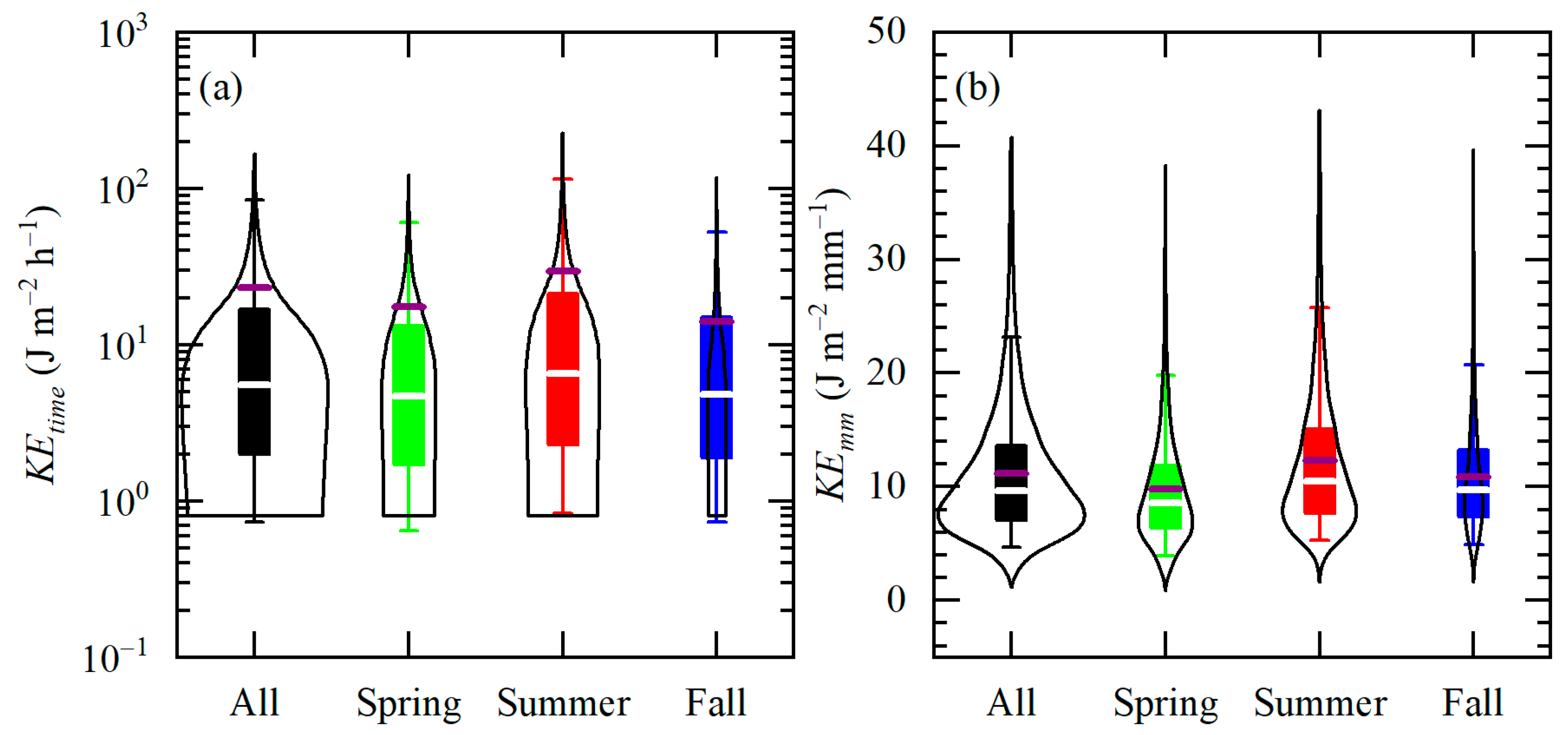
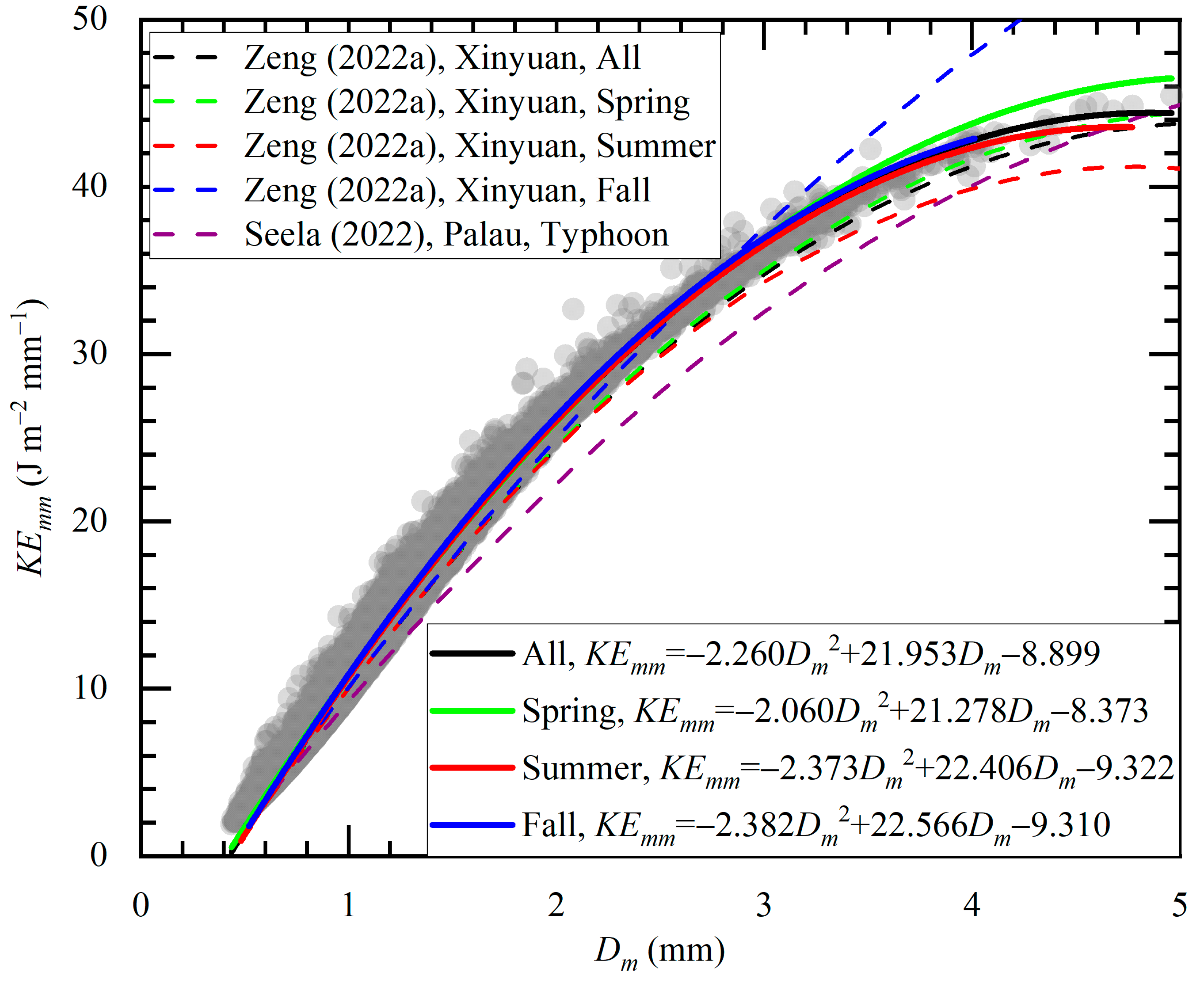
Mean KE_time was the largest (smallest) at 29.418 (14.006) J m⁻² h⁻¹ in summer (fall), and mean KE_mm was the largest (smallest) at 12.307 (9.826) J m⁻² mm⁻¹ in summer (spring). Two RKEE schemes, KE_time–R and KE_mm–D_m, were established as KE_time = 12.495R^1.285 and KE_mm = −2.260D_m² + 21.953D_m − 8.899 for the entire data, respectively, and both showed seasonal variations. By comparing the estimated KE_time and KE_mm of the established RKEE schemes with the KE_time and KE_mm obtained directly from DSD based on the CC, RMSE, and NMAE, it was confirmed that the RKEE schemes performed well for the entire dataset and different seasons.

(2)

For both stratiform and convective rainfall under both BR03 and BR09 (i.e., BR09_S, BR09_C, BR03_S, and BR03_C), mean KE_time (17.535, 405.907, 28.590, and 379.887 J m⁻² h⁻¹, respectively), and KE_mm (11.677, 32.209, 13.342, and 24.920 J m⁻² mm⁻¹, respectively) in summer were larger than those in other seasons. The KE_time–R and KE_mm–D_m relationships for stratiform and convective rainfall under BR09 and BR03 were established and showed seasonal variations. The evaluation results showed that both types of RKEE schemes had excellent estimation performances for rainfall KE under BR09_S, BR09_C, BR03_S, and BR03_C, particularly the KE_mm–D_m relationship.

(3)

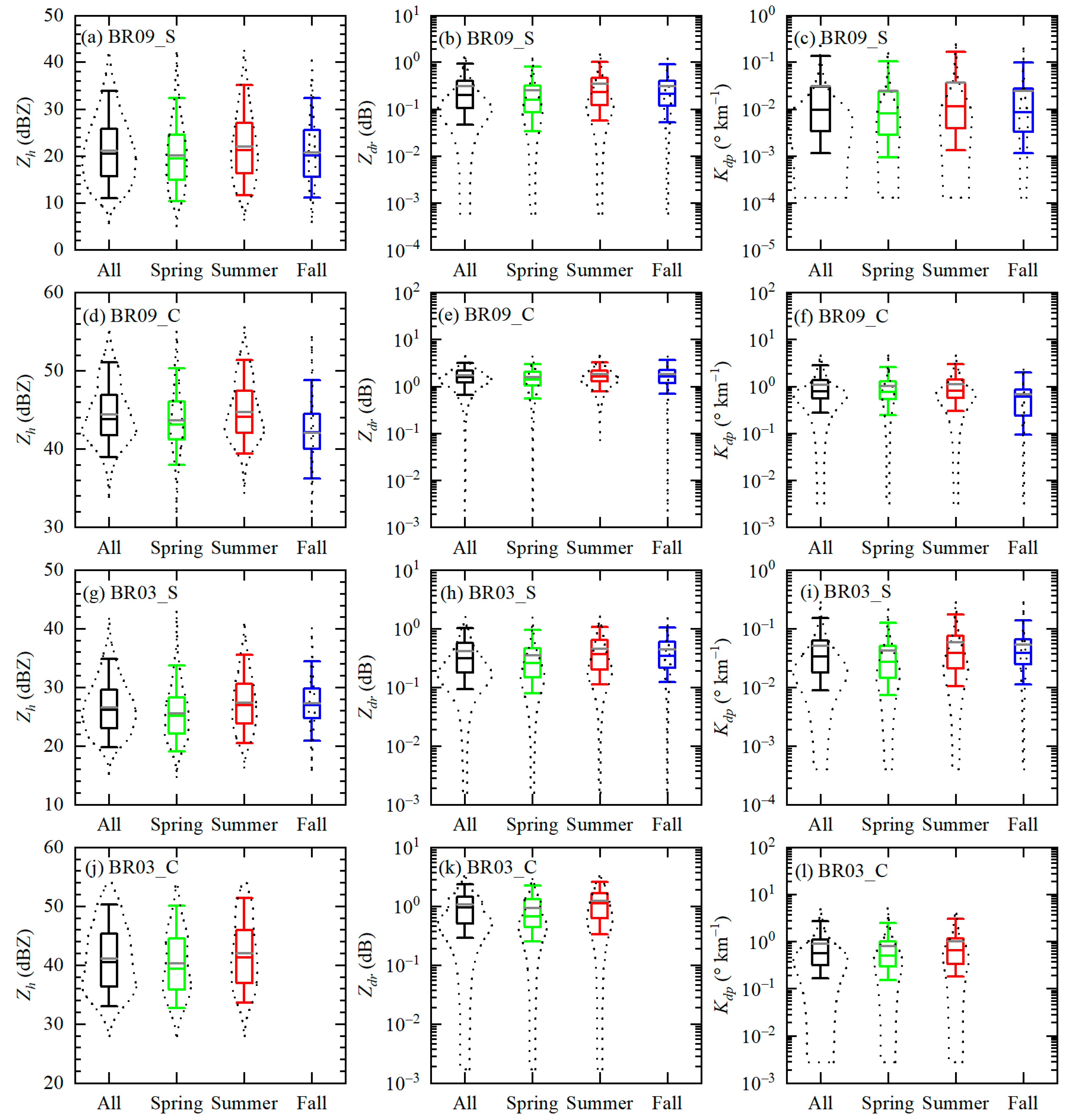
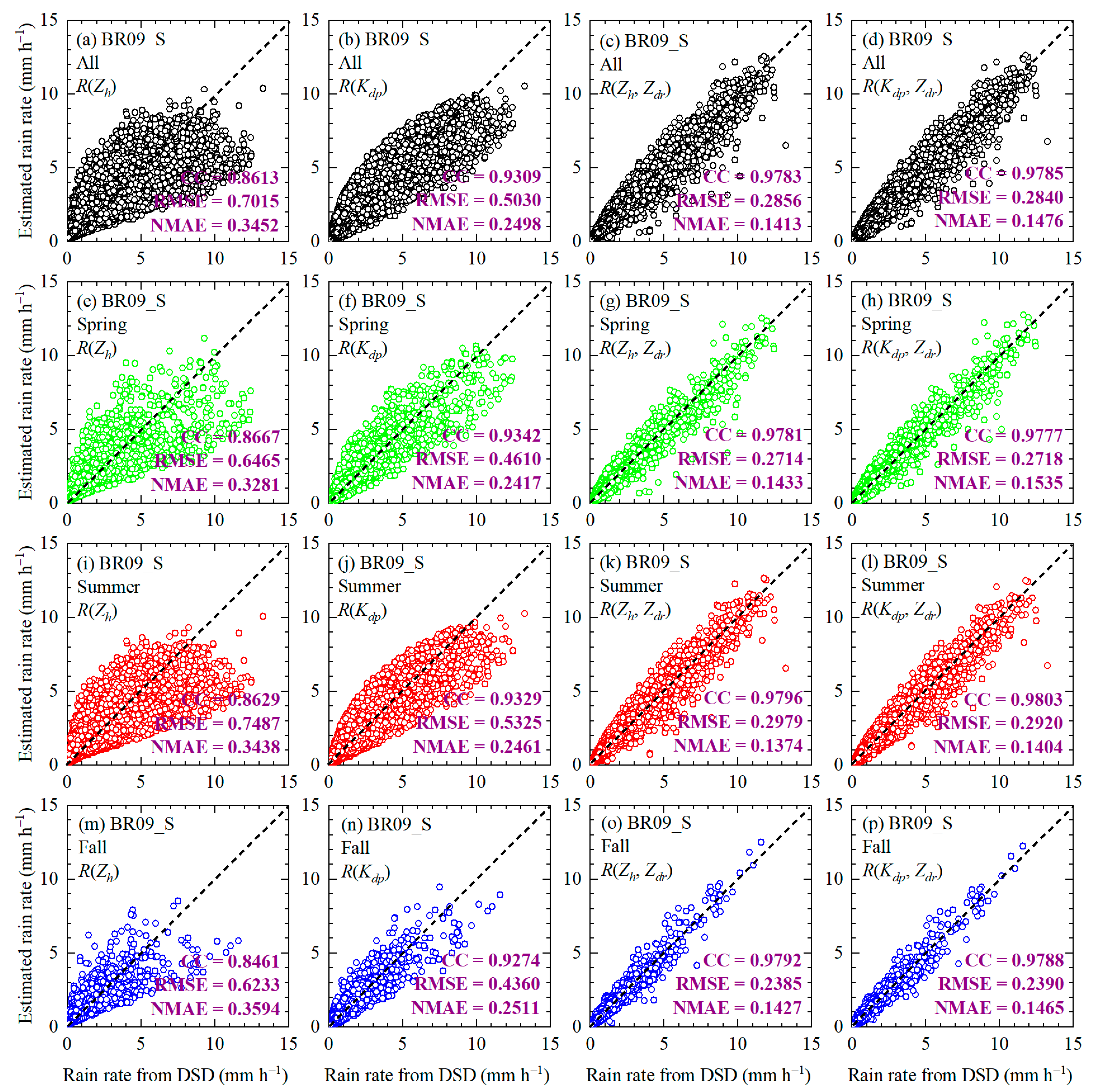
For the entire dataset and three seasons, the mean Z_h was close to 21.6, 20.4, 22.7, and 20.9 dBZ, respectively. The mean Z_dr was largest (smallest) at 0.388 (0.269) dB in summer (spring), and the mean K_dp was largest (smallest) at 0.070 (0.029) ° km⁻¹ in summer (fall). Dual-polarization radar QPE algorithms differed seasonally. The coefficient f(g) of the R(Z_h) algorithm varied from 0.064 (0.491) to 0.072 (0.516), and the coefficient h(i) of the R(K_dp) algorithm varied from 13.097 (0.649) to 14.655 (0.680) between different seasons. For the entire dataset and all seasons, the double-parameter algorithms were better than the single-parameter algorithms. Moreover, the R(K_dp, Z_dr) [R(K_dp)] algorithm was superior to the R(Z_h, Z_dr) [R(Z_h)] algorithm.

(4)

Differences were found in different seasons and types of rainfall under BR03 and BR09 for the four types of dual-polarization radar QPE algorithms. For different seasons and rainfall types in BR03 and BR09, the double-parameter algorithms were better than the single-parameter algorithms, and the R(K_dp) algorithm was superior to the R(Z_h) algorithm. For BR09_C, the R(Z_h, Z_dr) algorithm performed the best (worst) in spring (fall), while for BR09_S, the R(K_dp, Z_dr) algorithm performed the best (worst) in summer (spring). For BR03_C (BR03_S), the double-parameter algorithm exhibited the best performance in spring (summer).

The results of this study show that it is necessary to consider different rainfall types and seasons, as well as classification methods for rainfall types, when applying RKEE and dual-polarization radar QPE. In this process, choosing a suitable estimator (KE_time(R), KE_mm(D_m), R(K_dp), R(Z_h), R(K_dp,Z_dr), or R(Z_h,Z_dr)) is key to improving the accuracy of estimating rainfall KE and R. However, it is necessary to establish a denser DSD observation network and to use various satellite observations to further obtain RKEE schemes and dual-polarization radar QPE algorithms over the Tianshan Mountains from a larger spatial scale.

References

1. Rosenfeld, D.; Ulbrich, C.W. Cloud microphysical properties, processes, and rainfall estimation opportunities. Meteorol. Monogr. 2003, 30, 237–258. [Google Scholar]
2. Zhang, G.; Sun, J.; Brandes, E.A. Improving parameterization of rain microphysics with disdrometer and radar observations. J. Atmos. Sci. 2006, 63, 1273–1290. [Google Scholar]
3. Mason, B.J. Physics of clouds and precipitation. Nature 1954, 174, 957–959. [Google Scholar]
4. Fornis, R.L.; Vermeulen, H.R.; Nieuwenhuis, J.D. Kinetic Energy–Rainfall Intensity Relationship for Central Cebu, Philippines for Soil Erosion Studies. J. Hydrol. 2005, 300, 20–32. [Google Scholar] [CrossRef]
5. Van, L.N.; Le, X.-H.; Nguyen, G.V.; Yeon, M.; May, D.T.T.; Lee, G. Comprehensive Relationships between Kinetic Energy and Rainfall Intensity Based on Precipitation Measurements from an OTT Parsivel2 Optical Disdrometer. Front. Environ. Sci. 2022, 10, 985516. [Google Scholar]
6. Lim, Y.S.; Kim, J.K.; Kim, J.W.; Park, B.I.; Kim, M.S. Analysis of the Relationship between the Kinetic Energy and Intensity of Rainfall in Daejeon, Korea. Quat. Int. 2015, 384, 107–117. [Google Scholar] [CrossRef]
7. Kinnell, P.I.A. Rainfall Intensity-Kinetic Energy Relationships for Soil Loss Prediction1. Soil Sci. Soc. Am. J. 1981, 45, 153. [Google Scholar]
8. Steiner, M.; Smith, J.A. Reflectivity, Rain Rate, and Kinetic Energy Flux Relationships Based on Raindrop Spectra. J. Appl. Meteorol. 2000, 39, 1923–1940. [Google Scholar] [CrossRef]
9. Seela, B.K.; Janapati, J.; Kalath Unnikrishnan, C.; Lin, P.-L.; Le Loh, J.; Chang, W.-Y.; Kumar, U.; Reddy, K.K.; Lee, D.-I.; Venkatrami Reddy, M. Raindrop Size Distributions of North Indian Ocean Tropical Cyclones Observed at the Coastal and Inland Stations in South India. Remote Sens. 2021, 13, 3178. [Google Scholar] [CrossRef]
10. Ryzhkov, A.V.; Zrnic, D.S. Comparison of dual polarization radar estimators of rain. J. Atmos. Ocean. Technol. 1995, 12, 249–256. [Google Scholar] [CrossRef]
11. Liao, L.; Meneghini, R.; Tokay, A. Uncertainties of GPM DPR rain estimates caused by DSD parameterizations. J. Appl. Meteor. Climatol. 2014, 53, 2524–2537. [Google Scholar] [CrossRef]
12. Chen, B.; Yang, J.; Pu, J. Statistical characteristics of raindrop size distribution in the Meiyu season observed in eastern China. J. Meteorol. Soc. Jpn. 2013, 91, 215–227. [Google Scholar] [CrossRef]
13. Zhang, Z.; Li, H.; Li, D.; Qi, Y. Spatial Variability of Raindrop Size Distribution at Beijing City Scale and Its Implications for Polarimetric Radar QPE. Remote Sens. 2023, 15, 3964. [Google Scholar] [CrossRef]
14. Chen, G.; Zhao, K.; Zhang, G.; Huang, H.; Liu, S.; Wen, L.; Yang, Z.; Yang, Z.; Xu, L.; Zhu, W. Improving Polarimetric C-Band Radar Rainfall Estimation with Two-Dimensional Video Disdrometer Observations in Eastern China. J. Hydrometeorol. 2017, 18, 1375–1391. [Google Scholar] [CrossRef]
15. Cao, Q.; Zhang, G.; Brandes, E.A.; Schuur, T.J. Polarimetric radar rain estimation through retrieval of drop size distribution using a Bayesian approach. J. Appl. Meteorol. Climatol. 2010, 49, 973–990. [Google Scholar] [CrossRef]
16. Ulbrich, C.W. Natural variations in the analytical form of the raindrop size distribution. J. Clim. Appl. Meteorol. 1983, 22, 1764–1775. [Google Scholar] [CrossRef]
17. Tokay, A.; Short, D.A. Evidence from tropical raindrop spectra of the origin of rain from stratiform versus convective clouds. J. Appl. Meteorol. 1996, 35, 355–371. [Google Scholar] [CrossRef]
18. Bringi, V.N.; Chandrasekar, V.; Hubbert, J.; Gorgucci, E.; Randeu, W.L.; Schoenhuber, M. Raindrop size distribution in different climatic regimes from disdrometer and dual-polarized radar analysis. J. Atmos. Sci. 2003, 60, 354–365. [Google Scholar] [CrossRef]
19. Konwar, M.; Das, S.K.; Deshpande, S.M.; Chakravarty, K.; Goswami, B.N. Microphysics of clouds and rain over the Western Ghat. J. Geophys. Res. Atmos. 2014, 119, 6140–6159. [Google Scholar] [CrossRef]
20. Chen, B.; Hu, Z.; Liu, L.; Zhang, G. Raindrop Size Distribution Measurements at 4500 m on the Tibetan Plateau during TIPEX-III. J. Geophys. Res. Atmos. 2017, 12211, 11092–12006. [Google Scholar]
21. Seela, B.K.; Janapati, J.; Lin, P.-L.; Reddy, K.K.; Shirooka, R.; Wang, P.K. A Comparison Study of Summer Season Raindrop Size Distribution between Palau and Taiwan, Two Islands in Western Pacific. J. Geophys. Res. Atmos. 2017, 122, 11–787. [Google Scholar] [CrossRef]
22. Suh, S.-H.; You, C.-H.; Lee, D.-I. Climatological characteristics of raindrop size distributions in Busan, Republic of Korea. Hydrol. Earth Syst. Sci. 2016, 20, 193–207. [Google Scholar] [CrossRef]
23. Wen, L.; Zhao, K.; Chen, G. Drop size distribution characteristics of seven typhoons in China. J. Geophys. Res. Atmos. 2018, 123, 6529–6548. [Google Scholar] [CrossRef]
24. Zheng, J.; Liu, L.; Chen, H. Characteristics of warm clouds and precipitation in South China during the pre-flood season using datasets from a cloud radar, a ceilometer, and a disdrometer. Remote Sens. 2019, 11, 3045. [Google Scholar] [CrossRef]
25. Zhang, A.; Hu, J.; Chen, S. Statistical characteristics of raindrop size distribution in the monsoon season observed in southern China. Remote Sens. 2019, 11, 432. [Google Scholar] [CrossRef]
26. Wen, L.; Zhao, K.; Zhang, G. Statistical characteristics of raindrop size distributions observed in East China during the Asian summer monsoon season using 2-D video disdrometer and Micro Rain Radar data. J. Geophys. Res. Atmos. 2016, 121, 2265–2282. [Google Scholar] [CrossRef]
27. Pu, K.; Liu, X.; Wu, Y.; Hu, S.; Liu, L.; Gao, T. A comparison study of raindrop size distribution among five sites at the urban scale during the East Asian rainy season. J. Hydrol. 2020, 590, 125500. [Google Scholar] [CrossRef]
28. Wen, L.; Zhao, K.; Wang, M. Seasonal variations of observed raindrop size distribution in East China. Adv. Atmos. Sci. 2019, 36, 346–362. [Google Scholar] [CrossRef]
29. Zhang, H.; Zhang, Y.; He, H. Comparison of raindrop size distributions in a midlatitude continental squall line during different stages as measured by Parsivel over East China. J. Appl. Meteorol. Climatol. 2017, 56, 2097–2111. [Google Scholar] [CrossRef]
30. Luo, L.; Guo, J.; Chen, H. Microphysical characteristics of rainfall observed by a 2DVD disdrometer during different seasons in Beijing, China. Remote Sens. 2021, 13, 2303. [Google Scholar] [CrossRef]
31. Ma, Y.; Ni, G.; Chandra, C.V. Statistical characteristics of raindrop size distribution during rainy seasons in the Beijing urban area and implications for radar rainfall estimation. Hydrol. Earth Syst. Sci. 2019, 23, 4153–4170. [Google Scholar] [CrossRef]
32. Ji, L.; Chen, H.N.; Li, L.; Chen, B.J.; Xiao, X.; Chen, M.; Zhang, G.F. Raindrop size distributions and rain characteristics observed by a PARSIVEL disdrometer in Beijing, Northern China. Remote Sens. 2019, 11, 1479. [Google Scholar] [CrossRef]
33. Wang, G.; Zhou, R.; Zhaxi, S.; Liu, S. Raindrop size distribution measurements on the Southeast Tibetan Plateau during the STEP project. Atmos. Res. 2021, 249, 105311. [Google Scholar] [CrossRef]
34. Wang, G.; Li, R.; Sun, J. Comparative analysis of the characteristics of rainy season raindrop size distributions in two typical regions of the Tibetan Plateau. Adv. Atmos. Sci. 2022, 39, 1062–1078. [Google Scholar] [CrossRef]
35. Janapati, J.; Seela, B.K.; Lin, P.L.; Lan, C.H.; Tu, C.C.; Kumar, U.; Huang, M.Q. An assessment of rainfall kinetic energy functional relationships with GPM DPR. J. Hydrol. 2023, 617, 128754. [Google Scholar] [CrossRef]
36. Wu, H.; Niu, S.; Zhou, Y.; Sun, J.; Lv, J.; He, Y. Characteristics of Raindrop Size Distributions in the Southwest Mountain Areas of China According to Seasonal Variation and Rain Types. Remote Sens. 2023, 15, 1246. [Google Scholar] [CrossRef]
37. Marshall, J.S.; Palmer, W.M. The distribution of raindrops with size. J. Meteor. 1948, 5, 165–166. [Google Scholar] [CrossRef]
38. Fulton, R.A.; Breidenbach, J.P.; Seo, D.-J. The WSR-88D Rainfall Algorithm. Weather. Forecast. 1998, 13, 377–395. [Google Scholar] [CrossRef]
39. Atlas, D.; Ulbrich, C.W.; Marks, F.D. Systematic variation of drop size and radar-rainfall relations. J. Geophys. Res. 1999, 104, 6155–6169. [Google Scholar] [CrossRef]
40. Ulbrich, C.W.; Atlas, D. Microphysics of raindrop size spectra: Tropical continental and maritime storms. J. Appl. Meteor. Climatol. 2007, 46, 1777–1791. [Google Scholar] [CrossRef]
41. Janapati, J.; Seela, B.K.; Lin, P.-L. Raindrop size distribution characteristics of Indian and Pacific Ocean tropical cyclones observed at India and Taiwan sites. J. Meteor. Soc. Jpn. 2020, 98, 299–317. [Google Scholar] [CrossRef]
42. Janapati, J.; Seela, B.K.; Lin, P.-L.; Lee, M.-T.; Joseph, E. Microphysical features of typhoon and non-typhoon rainfall observed in Taiwan, an island in the northwestern Pacific. Hydrol. Earth Syst. Sci. 2021, 25, 4025–4040. [Google Scholar] [CrossRef]
43. Kim, H.-J.; Jung, W.; Suh, S.-H.; Lee, D.-I.; You, C.-H. The Characteristics of raindrop size distribution at windward and leeward side over mountain area. Remote Sens. 2022, 14, 2419. [Google Scholar] [CrossRef]
44. Li, R.; Wang, G.; Zhou, R.; Zhang, J.; Liu, L. Seasonal variation in microphysical characteristics of precipitation at the entrance of water vapor channel in Yarlung Zangbo Grand Canyon. Remote Sens. 2022, 14, 3149. [Google Scholar] [CrossRef]
45. Cifelli, R.; Chandrasekar, V.; Lim, S.; Kennedy, P.C.; Wang, Y.; Rutledge, S.A. A new dual-polarization radar rainfall algorithm: Application in Colorado precipitation events. J. Atmos. Ocean. Technol. 2011, 28, 352–364. [Google Scholar] [CrossRef]
46. You, C.-H.; Kang, M.; Lee, D.-I. Rainfall estimation by S-band polarimetric radar in Korea. Part I: Preprocessing and preliminary results. Meteorol. Appl. 2014, 21, 975–983. [Google Scholar] [CrossRef]
47. Brandes, E.A.; Zhang, G.; Vivekanandan, J. Experiments in rainfall estimation with a polarimetric radar in a subtropical environment. J. Appl. Meteorol. 2002, 41, 674–685. [Google Scholar] [CrossRef]
48. Li, Q.; Wei, J.; Yin, J.; Qiao, Z.; Cao, J.; Shi, Y. Microphysical characteristics of raindrop size distribution and implications for radar rainfall estimation over the northeastern Tibetan Plateau. J. Geophys. Res. Atmos. 2022, 127, e2021JD035575. [Google Scholar] [CrossRef]
49. You, C.-H.; Suh, S.-H.; Jung, W.; Kim, H.-J.; Lee, D.-I. Dual-Polarization Radar-Based Quantitative Precipitation Estimation of Mountain Terrain Using Multi-Disdrometer Data. Remote Sens. 2022, 14, 2290. [Google Scholar] [CrossRef]
50. Zhang, J.B.; Deng, Z.F. A Generality of Rainfall in Xinjiang; Meteorological Press: Beijing, China, 1987; pp. 1–10. (In Chinese) [Google Scholar]
51. Yang, L.M.; Li, X.; Zhang, G.X. Some advances and problems in the study of heavy rain in Xinjiang. Clim. Environ. Res. 2011, 16, 188–198. (In Chinese) [Google Scholar]
52. Zeng, Y.; Yang, L. Triggering mechanism of an extreme rainstorm process near the Tianshan Mountains in Xinjiang, an arid region in China, based on a numerical simulation. Adv. Meteorol. 2020, 2020, 8828060. [Google Scholar] [CrossRef]
53. Zeng, Y.; Yang, L.; Zhang, Z.; Tong, Z.; Li, J.; Liu, F.; Zhang, J.; Jiang, Y. Characteristics of clouds and raindrop size distribution in Xinjiang, using cloud radar datasets and a disdrometer. Atmosphere 2020, 11, 1382. [Google Scholar] [CrossRef]
54. Zeng, Y.; Yang, L.; Tong, Z.; Jiang, Y.; Zhang, Z.; Zhang, J.; Zhou, Y.; Li, J.; Liu, F.; Liu, J. Statistical characteristics of raindrop size distribution during rainy seasons in Northwest China. Adv. Meteorol. 2021, 2021, 6667786. [Google Scholar] [CrossRef]
55. Zeng, Y.; Tong, Z.; Jiang, Y.; Zhou, Y. Microphysical characteristics of seasonal rainfall observed by a Parsivel disdrometer in the Tianshan Mountains, China. Atmos. Res. 2022, 280, 106459. [Google Scholar] [CrossRef]
56. Zeng, Y.; Yang, L.; Tong, Z.; Jiang, Y.; Chen, P.; Zhou, Y. Characteristics and applications of summer season raindrop size distributions based on a PARSIVEL2 disdrometer in the western Tianshan Mountains (China). Remote Sens. 2022, 14, 3988. [Google Scholar] [CrossRef]
57. Zeng, Y.; Yang, L.; Zhou, Y.; Tong, Z.; Jiang, Y.; Chen, P. Characteristics of orographic raindrop size distribution in the Tianshan Mountains, China. Atmos. Res. 2022, 278, 106332. [Google Scholar] [CrossRef]
58. Zeng, Y.; Yang, L.; Zhou, Y.; Tong, Z.; Jiang, Y. Statistical characteristics of summer season raindrop size distribution in the western and central Tianshan Mountains in China. J. Meteor. Soc. Jpn. 2022, 100, 855–872. [Google Scholar] [CrossRef]
59. Zeng, Y.; Yang, L.; Li, J.; Jiang, Y.; Tong, Z.; Li, X.; Li, H.; Liu, J.; Lu, X.; Zhou, Y. Seasonal variation of microphysical characteristics for different rainfall types in the Tianshan Mountains of China. Atmos. Res. 2023, 295, 107024. [Google Scholar] [CrossRef]
60. Zeng, Y.; Li, J.; Yang, L.; Li, H.; Li, X.; Tong, Z.; Jiang, Y.; Liu, J.; Zhang, J.; Zhou, Y. Microphysical Characteristics of Raindrop Size Distribution and Implications for Dual-Polarization Radar Quantitative Precipitation Estimations in the Tianshan Mountains, China. Remote Sens. 2023, 15, 2668. [Google Scholar] [CrossRef]
61. Chen, P.; Wang, P.; Li, Z.; Yang, Y.; Jia, Y.; Yang, M.; Peng, J.; Li, H. Raindrop Size Distribution Characteristics of Heavy Precipitation Events Based on a PWS100 Disdrometer in the Alpine Mountains, Eastern Tianshan, China. Remote Sens. 2023, 15, 5068. [Google Scholar] [CrossRef]
62. Bringi, V.N.; Williams, C.R.; Thurai, M. Using dual-polarized radar and dual-frequency profiler for DSD characterization: A case study from Darwin, Australia. J. Atmos. Oceanic Technol. 2009, 26, 2107–2122. [Google Scholar] [CrossRef]
63. Löffler-Mang, M.; Joss, J. An optical disdrometer for measuring size and velocity of hydrometeors. J. Atmos. Ocean. Technol. 2000, 17, 130–139. [Google Scholar] [CrossRef]
64. Yuter, S.E.; Kingsmill, D.E.; Nance, L.B.; Löffler-Mang, M. Observations of precipitation size and fall speed characteristics within coexisting rain and wet snow. J. Appl. Meteorol. 2006, 45, 1450–1464. [Google Scholar] [CrossRef]
65. Huang, C.; Chen, S.; Zhang, A.; Pang, Y. Statistical characteristics of raindrop size distribution in monsoon season over South China Sea. Remote Sens. 2021, 13, 2878. [Google Scholar] [CrossRef]
66. Chen, B.; Yang, J.; Gao, R.; Zhu, K.; Zou, C.; Gong, Y.; Zhang, R. Vertical variability of the raindrop size distribution in typhoons observed at the Shenzhen 356-m meteorological tower. J. Atmos. Sci. 2020, 77, 4171–4187. [Google Scholar] [CrossRef]
67. Fu, Z.; Dong, X.; Zhou, L.; Cui, W.; Wang, J.; Wan, R.; Leng, L.; Xi, B. Statistical characteristics of raindrop size distributions and parameters in Central China during the Meiyu seasons. J. Geophys. Res. Atmos. 2020, 125, e2019JD031954. [Google Scholar] [CrossRef]
68. Liu, X.; Xue, L.; Chen, B.; Zhang, Y. Characteristics of raindrop size distributions in Chongqing observed by a dense network of disdrometers. J. Geophys. Res. Atmos. 2021, 126, e2021JD035172. [Google Scholar] [CrossRef]
69. Sreekanth, T.S.; Varikoden, H.; Sukumar, N.; Mohan Kumar, G. Microphysical characteristics of rainfall during different seasons over a coastal tropical station using disdrometer. Hydrol. Process. 2017, 31, 2556–2565. [Google Scholar] [CrossRef]
70. Tokay, A.; Petersen, W.A.; Gatlin, P.; Wingo, M. Comparison of raindrop size distribution measurements by collocated disdrometers. J. Atmos. Ocean. Technol. 2013, 30, 1672–1690. [Google Scholar] [CrossRef]
71. Friedrich, K.; Higgins, S.; Masters, F.J.; Lopez, C.R. Articulating and stationary PARSIVEL disdrometer measurements in conditions with strong Winds and heavy rainfall. J. Atmos. Oceanic Technol. 2013, 30, 2063–2080. [Google Scholar] [CrossRef]
72. Salles, C.; Poesen, J.; Sempere-Torres, D. Kinetic energy of rain and its functional relationship with intensity. J. Hydrol. 2002, 257, 256–270. [Google Scholar] [CrossRef]
73. Van Dijk, A.; Bruijnzeel, L.A.; Rosewell, C.J. Rainfall intensity–kinetic energy relationships: A critical literature appraisal. J. Hydrol. 2002, 261, 1–23. [Google Scholar] [CrossRef]
74. Tokay, A.; Wolff, D.B.; Petersen, W.A. Evaluation of the new version of the laser-optical disdrometer, OTT Parsivel2. J. Atmos. Ocean. Technol. 2014, 31, 1276–1288. [Google Scholar] [CrossRef]
75. Battaglia, A.; Rustemeier, E.; Tokay, A. PARSIVEL snow observations: A critical assessment. J. Atmos. Oceanic Technol. 2010, 27, 333–344. [Google Scholar] [CrossRef]
76. Testud, J.; Oury, S.; Amayenc, P.; Black, R.A. The concept of “normalized” distributions to describe raindrop spectra: A tool for cloud physics and cloud remote sensing. J. Appl. Meteorol. 2001, 40, 1118–1140. [Google Scholar] [CrossRef]
77. Kalogiros, J.; Anagnostou, M.N.; Anagnostou, E.N. Optimum estimation of rain microphysical parameters from X-band dual-polarization radar observables. IEEE Trans. Geosci. Remote Sens. 2013, 51, 3063–3076. [Google Scholar] [CrossRef]
78. Leinonen, J. High-level interface to T-matrix scattering calculations: Architecture, capabilities and limitations. Opt. Express 2014, 22, 1655–1660. [Google Scholar] [CrossRef]
79. Waterman, P.C. Matrix formulation of electromagnetic scattering. Proc. IEEE 1965, 53, 805–812. [Google Scholar] [CrossRef]
80. Tokay, A.; Short, D.A.; Williams, C.R.; Ecklund, W.L.; Gage, K.S. Tropical Rainfall Associated with Convective and Stratiform Clouds: Intercomparison of Disdrometer and Profiler Measurements. J. Appl. Meteorol. 1999, 38, 302–320. [Google Scholar] [CrossRef]
81. Dolan, B.; Fuchs, B.; Rutledge, S.A.; Barnes, E.A.; Thompson, E.J. Primary modes of global drop size distributions. J. Atmos. Sci. 2018, 75, 1453–1476. [Google Scholar] [CrossRef]
82. Lee, M.T.; Lin, P.L.; Chang, W.Y.; Seela, B.K.; Janapati, J. Microphysical characteristics and types of precipitation for different seasons over North Taiwan. J. Meteor. Soc. Jpn. 2019, 97, 841–865. [Google Scholar] [CrossRef]
83. Seela, B.K.; Janapati, J.; Lin, P.-L.; Lan, C.-H.; Shirooka, R.; Hashiguchi, H.; Reddy, K.K. Raindrop Size Distribution Characteristics of the Western Pacific Tropical Cyclones Measured in the Palau Islands. Remote Sens. 2022, 14, 470. [Google Scholar] [CrossRef]
84. Guo, Z.; Hu, S.; Liu, X.; Chen, X.; Zhang, H.; Qi, T.; Zeng, G. Improving S-band polarimetric radar monsoon rainfall estimation with two-dimensional video disdrometer observations in South China. Atmosphere 2021, 12, 831. [Google Scholar] [CrossRef]
Figure 1. (a) Topography (m) and location of the Tianshan Mountains, and (b) locations of Zhaosu (red dot) and Xinyuan (black dot; Zeng et al. [55]).
Remotesensing 16 03859 g001aRemotesensing 16 03859 g001b
Figure 2. Seasonal variations in the distributions of (a) KEtime and (b) KEmm at Zhaosu.
Remotesensing 16 03859 g002
Figure 3. Scatterplots of KEtime vs. R for the entire data and the fitted KEtimeR relationship across seasons at Zhaosu. Dashed lines represent the KEtimeR relationship reported by Zeng et al. [55], Seela et al. [83], and Wu et al. [36].
Remotesensing 16 03859 g003
Figure 4. Scatterplots of KEmm vs. Dm for the entire data and the seasonal variation in fitted KEmmDm at Zhaosu. Dashed lines represent the KEmmDm relationship reported by Zeng et al. [55] and Seela et al. [83].
Remotesensing 16 03859 g004
Figure 5. Scatterplot of estimated KEtime from RKEE schemes versus KEtime calculated from DSD for (a) the entire data, (b) spring, (c) summer, and (d) fall at Zhaosu. Scatterplot of estimated KEmm from RKEE schemes versus the KEmm calculated from DSD for (e) the entire data, (f) spring, (g) summer, and (h) fall at Zhaosu in Tianshan Mountains. Black dashed lines represent the 1:1 relationship.
Remotesensing 16 03859 g005
Figure 6. Violin plots of seasonal variations in KEtime under (a) BR09_S, (c) BR09_C, (e) BR03_S, and (g) BR03_C, and violin plots of seasonal variations in KEmm under (b) BR09_S, (d) BR09_C, (f) BR03_S, and (h) BR03_C at Zhaosu.
Remotesensing 16 03859 g006
Figure 7. Scatterplots of KEtime vs. R for the entire data and the seasonal variation of the fitted KEtimeR relationship at Zhaosu under (a) BR09_S, (b) BR09_C, (c) BR03_S, and (d) BR03_C.
Remotesensing 16 03859 g007
Figure 8. Scatterplot of estimated KEtime from RKEE schemes versus KEtime calculated from DSD for (a) the entire data, (e) spring, (i) summer, and (m) fall under BR09_S; those for (b) the entire data, (f) spring, (j) summer, and (n) fall under BR09_C; those for (c) the entire data, (g) spring, (k) summer, and (o) fall under BR03_S; and those for (d) the entire data, (h) spring, and (l) summer under BR03_C at Zhaosu. Black dashed lines represent the 1:1 relationship.
Remotesensing 16 03859 g008
Figure 9. Scatterplots of KEmm vs. Dm for the entire data and the fitted KEmmDm relationship across seasons at Zhaosu under (a) BR09_S, (b) BR09_C, (c) BR03_S, and (d) BR03_C.
Remotesensing 16 03859 g009
Figure 10. Scatterplot of estimated KEmm from RKEE schemes versus KEmm calculated from DSD for (a) the entire data, (e) spring, (i) summer, and (m) fall under BR09_S; for (b) the entire data, (f) spring, (j) summer, and (n) fall under BR09_C; for (c) the entire data, (g) spring, (k) summer, and (o) fall under BR03_S; and for (d) the entire data, (h) spring, and (l) summer under BR03_C at Zhaosu. Black dashed lines represent the 1:1 relationship.
Remotesensing 16 03859 g010
Figure 11. Seasonal variations in the distributions of (a) Zh, (b) Zdr, and (c) Kdp at Zhaosu.
Remotesensing 16 03859 g011
Figure 12. Scatterplot of estimated R based on the R(Zh) algorithm for (a) the entire data, (e) spring, (i) summer, and (m) fall; estimated R based on the R(Kdp) algorithm for (b) the entire data, (f) spring, (j) summer, and (n) fall; estimated R based on the R(Zh,Zdr) algorithm for (c) the entire data, (g) spring, (k) summer, and (o) fall; and estimated R based on the R(Kdp,Zdr) algorithm for (d) the entire data, (h) spring, (l) summer, and (p) fall versus calculated R according to Equation (4) at Zhaosu. Black dashed lines represent the 1:1 relationship.
Remotesensing 16 03859 g012
Figure 13. Seasonal variations in the distributions of Zh under (a) BR09_S, (d) BR09_C, (g) BR03_S, and (j) BR03_C; those of Zdr under (b) BR09_S, (e) BR09_C, (h) BR03_S, and (k) BR03_C; and those of Kdp under (c) BR09_S, (f) BR09_C, (i) BR03_S, and (l) BR03_C at Zhaosu.
Remotesensing 16 03859 g013
Figure 14. Scatterplot of estimated R based on the R(Zh) algorithm during BR09_S for (a) the entire data, (e) spring, (i) summer, and (m) fall; that based on the R(Kdp) algorithm during BR09_S for (b) the entire data, (f) spring, (j) summer, and (n) fall; that based on the R(Zh,Zdr) algorithm during BR09_S for (c) the entire data, (g) spring, (k) summer, and (o) fall; and that based on the R(Kdp,Zdr) algorithm during BR09_S for (d) the entire data, (h) spring, (l) summer, and (p) fall versus calculated R according to Equation (4) at Zhaosu. Black dashed lines represent the 1:1 relationship.
Remotesensing 16 03859 g014
Figure 15. Scatterplot of estimated R based on the R(Zh) algorithm during BR09_C for (a) the entire data, (e) spring, (i) summer, and (m) fall; that based on the R(Kdp) algorithm during BR09_C for (b) the entire data, (f) spring, (j) summer, and (n) fall; that based on the R(Zh,Zdr) algorithm during BR09_C for (c) the entire data, (g) spring, (k) summer, and (o) fall; and that based on the R(Kdp,Zdr) algorithm during BR09_C for (d) the entire data, (h) spring, (l) summer, and (p) fall versus calculated R according to Equation (4) at Zhaosu. Black dashed lines represent the 1:1 relationship.
Remotesensing 16 03859 g015
Figure 16. Scatterplot of estimated R based on the R(Zh) algorithm during BR03_S for (a) the entire data, (e) spring, (i) summer, and (m) fall; that based on the R(Kdp) algorithm during BR03_S for (b) the entire data, (f) spring, (j) summer, and (n) fall; that based on the R(Zh,Zdr) algorithm during BR03_S for (c) the entire data, (g) spring, (k) summer, and (o) fall; and that based on the R(Kdp,Zdr) algorithm during BR03_S for (d) the entire data, (h) spring, (l) summer, and (p) fall versus calculated R according to Equation (4) at Zhaosu. Black dashed lines represent the 1:1 relationship.
Remotesensing 16 03859 g016
Figure 17. Scatterplot of estimated R based on the R(Zh) algorithm during BR03_C for (a) the entire data, (e) spring, and (i) summer; that based on the R(Kdp) algorithm during BR03_C for (b) the entire data, (f) spring, and (j) summer; that based on the R(Zh,Zdr) algorithm during BR03_C for (c) the entire data, (g) spring, and (k) summer; and that based on the R(Kdp,Zdr) algorithm during BR03_C for (d) the entire data, (h) spring, and (l) summer versus calculated R according to Equation (4) at Zhaosu. Black dashed lines represent the 1:1 relationship.
Remotesensing 16 03859 g017