Abstract
Accurate estimation of gross primary production (GPP) of paddy rice fields is essential for understanding cropland carbon cycles, yet remains challenging due to spatial heterogeneity. In this study, we integrated high-resolution unmanned aerial vehicle (UAV) imagery into a leaf biochemical properties-based model for improving GPP estimation. The key parameter, maximum carboxylation rate at the top of the canopy (), was quantified using various spatial information representation methods, including mean (μref) and standard deviation (σref) of reflectance, gray-level co-occurrence matrix (GLCM)-based features, local binary pattern histogram (LBPH), and convolutional neural networks (CNNs). Our models were evaluated using a two-year eddy covariance (EC) system and UAV measurements. The result shows that incorporating spatial information can vastly improve the accuracy of and GPP estimation. CNN methods achieved the best estimation, with an R of 0.94, an RMSE of 19.44 μmol m−2 s−1, and an MdAPE of 11%, and further produced highly accurate GPP estimates, with an R of 0.92, an RMSE of 6.5 μmol m−2 s−1, and an MdAPE of 23%. The μref-GLCM texture features and μref-LBPH joint-driven models also gave promising results. However, σref contributed less to estimation. The Shapley value analysis revealed that the contribution of input features varied considerably across different models. The CNN model focused on nir and red-edge bands and paid much attention to the subregion with high spatial heterogeneity. The μref-LBPH joint-driven model mainly prioritized reflectance information. The μref-GLCM-based features joint-driven model emphasized the role of GLCM texture indices. As the first study to leverage the spatial information from high-resolution UAV imagery for GPP estimation, our work underscores the critical role of spatial information and provides new insight into monitoring the carbon cycle.
1. Introduction
Gross primary production (GPP) is the total amount of carbon compounds produced through plant photosynthesis and indicates the carbon sequestration capacity of ecosystems [1]. In cropland ecosystems, GPP is integral to yield formation [2]. Paddy rice, as an important staple food crop, occupies approximately 165.58 million hectares globally and sustains over half of the world population [3]. Therefore, accurate estimation of GPP in paddy rice cropland not only benefits the quantification of the carbon sequestration but also contributes to crop yield prediction [4].
Some classical models for GPP estimation have been developed over the past few decades, which can be categorized into the statistical model [5,6], the leaf biochemical properties-based model [7,8,9], the light use efficiency model [10,11], and the solar-induced chlorophyll fluorescence model [12,13]. These models have significantly advanced our understanding of the global carbon cycle. Among them, the leaf biochemical properties-based model, on the foundation of the Calvin cycle theory, elucidates the three steps of carbon sequestration in photosynthetic carbon reactions and has received much attention for its excellent physical interpretability.
In the leaf biochemical properties-based model, a major source of error in GPP estimation arises from the uncertainty in a key parameter, the leaf maximum carboxylation rate (normalized to 25 °C, ) [14]. indicates the enzyme activity of Rubisco. The substantial spatiotemporal variability of has long been observed [15,16]. Consequently, extensive efforts have been invested in quantifying the dynamics of to acquire an accurate GPP estimation. On the one hand, a number of biophysical and biochemical factors that mechanistically relate to , such as leaf nitrogen, leaf phosphorus, specific leaf area, leaf chlorophyll content, and leaf area index, have been identified [17,18,19,20]. On the other hand, the spectral information, including vegetation index, multispectral reflectance, hyperspectral reflectance, and fluorescence spectral information, has also shown promising potential for retrieving [21,22,23,24,25]. The abovementioned factors have been incorporated into the leaf biochemical properties-based model and significantly enhance the accuracy of GPP estimation [14].
At the field-scale, is a macroscopic feature within the specific spatial range, theoretically upscaled from leaf-level and thus determined by the spatial distribution of -related properties on underlying surfaces. However, the spatial information of -related properties on underlying surfaces has rarely been considered in previous studies. Traditional methods for measuring biophysical and biochemical factors, whether destructive or non-destructive, make it challenging to obtain precise spatial distributions. While satellite remote sensing offers widely accessible spectral images at a medium and low spatial resolution (10–30 m resolution) from platforms like Sentinel-2, Landsat 8 OLI and TIRS, Landsat ETM+, and Moderate-resolution Imaging Spectroradiometer (MODIS), this resolution is often insufficient for capturing the detailed spatial distribution of spectral properties. Moreover, satellite images are frequently disrupted by clouds, causing spatiotemporal discontinuities. These gaps in spatial information likely impede the accurate estimation of filed-scale . In contrast, the unmanned aerial vehicle (UAV) can capture high-resolution images even in cloudy conditions, offering better capability to describe the spatial distribution of spectral information. Therefore, UAV imagery holds great potential for extracting valuable spatial information to enhance field-scale estimation.
Due to the high-dimensional characteristics of UAV imagery, extracting meaningful information using traditional methods poses challenges. There are several approaches to extracting the spatial information from different perspectives. The standard deviation of the pixel values is the most straightforward indicator and is commonly used to quantify landscape heterogeneity [26]. However, it fails to provide other valuable information, such as the spatial distribution patterns. Texture analysis is a widely used approach in image processing. Texture is defined as the measure of coarseness, contrast, directionality, line-likeness, regularity, and roughness [27]. Various texture feature extraction methods have been proposed, including statistical approaches, structural approaches, transform-based approaches, model-based approaches, graph-based approaches, learning-based approaches, and entropy-based approaches [28]. Among these, the gray-level co-occurrence matrix (GLCM) is the most commonly used method [29] and has been widely applied in quantifying landscape patterns [30], as well as estimating various properties on underlying surfaces, such as leaf area index and biomass, from remote sensing images [31,32]. Other texture features, such as Fourier spectrum texture [33] and local binary pattern (LBP) texture [34,35], have also shown strong performance in quantifying specific landscape features, including leaf area index and orchard citrus fruits [36,37]. Despite the explicit and interpretable information extracted through texture analysis, this method may overlook large potential information in the raw images. The breakthrough in deep learning techniques, especially convolutional neural networks (CNNs), vastly enhances the capacity to extract image information. CNN utilizes the convolution and pooling operation to automatically detect the patterns across the entire image and thus can make full use of image information. CNN became a hot spot for its unparalleled performance regarding the image recognition issue [38]. Inspired by its success, the CNN technique is also employed to interpret remote sensing images. Notably, the combination of CNN and high-resolution UAV imagery shows a powerful capacity for retrieving valuable variables, such as crop yield [39] and leaf area index [40].
A few pioneering works have explored the retrieval of photosynthesis traits from images. Sun et al. [41] utilized several texture features, including the GLCM texture feature, LBP texture feature, and wavelet transform texture features, to monitor the leaf-scale net photosynthetic rate of potatoes. Deng et al. [42] proposed the optimal deep learning architecture to estimate the leaf-scale from hyperspectral images. These works suggest the potential of images for accurate estimation of photosynthetic traits. However, to the best of our knowledge, few studies have examined the effect of spatial information on field-scale estimation. As the first study that leveraged spatial information from high-resolution UAV imagery for and GPP estimation, we extracted the spatial information of the underlying surface from high-resolution images using various representation methods, including texture features and deep learning, to quantify the macroscopic feature, field-scale . The UAV-imagery-driven model was integrated into a classical leaf biochemical properties-based model for better GPP estimation. Our findings demonstrate the critical role of spatial information and provide new insight into monitoring GPP. The specific objective of this study is to (1) evaluate whether spatial information can improve the accuracy of field-scale , (2) build a UAV-imagery-driven hybrid framework for GPP estimation and validate its performance on the paddy rice field, and (3) see how spatial information contributes to field-scale estimation.
2. Materials and Methods
The research workflow is depicted in Figure 1, delineated into three distinct stages: (1) data preprocessing, including generating high-resolution UAV RGB orthomosaics and reflectance maps of UAV images, and half-hourly high-quality carbon flux measurements; (2) texture feature extraction from UAV images using four methods, including standard deviation features, GLCM-based texture features, LBP-based texture features, and CNN-based features; (3) model assessment, including evaluating the performance of 8 UAV imagery-driven models and their influences on GPP estimation, and analyzing the feature contribution of each model using the Shaley value method.
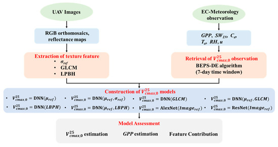
Figure 1.
Flowchart of the study (μref: the mean value of UAV reflectance; σref: the standard deviation value of UAV reflectance; GLCM: gray-level co-occurrence matrix-based texture features; LBPH: local binary pattern histogram texture feature; GPP: gross primary production; SWIN: incoming shortwave radiation; Ca: ambient CO2 concentration; Ta: air temperature; RH: relative humidity; u: wind speed).
2.1. Experiment Site and Data Collection
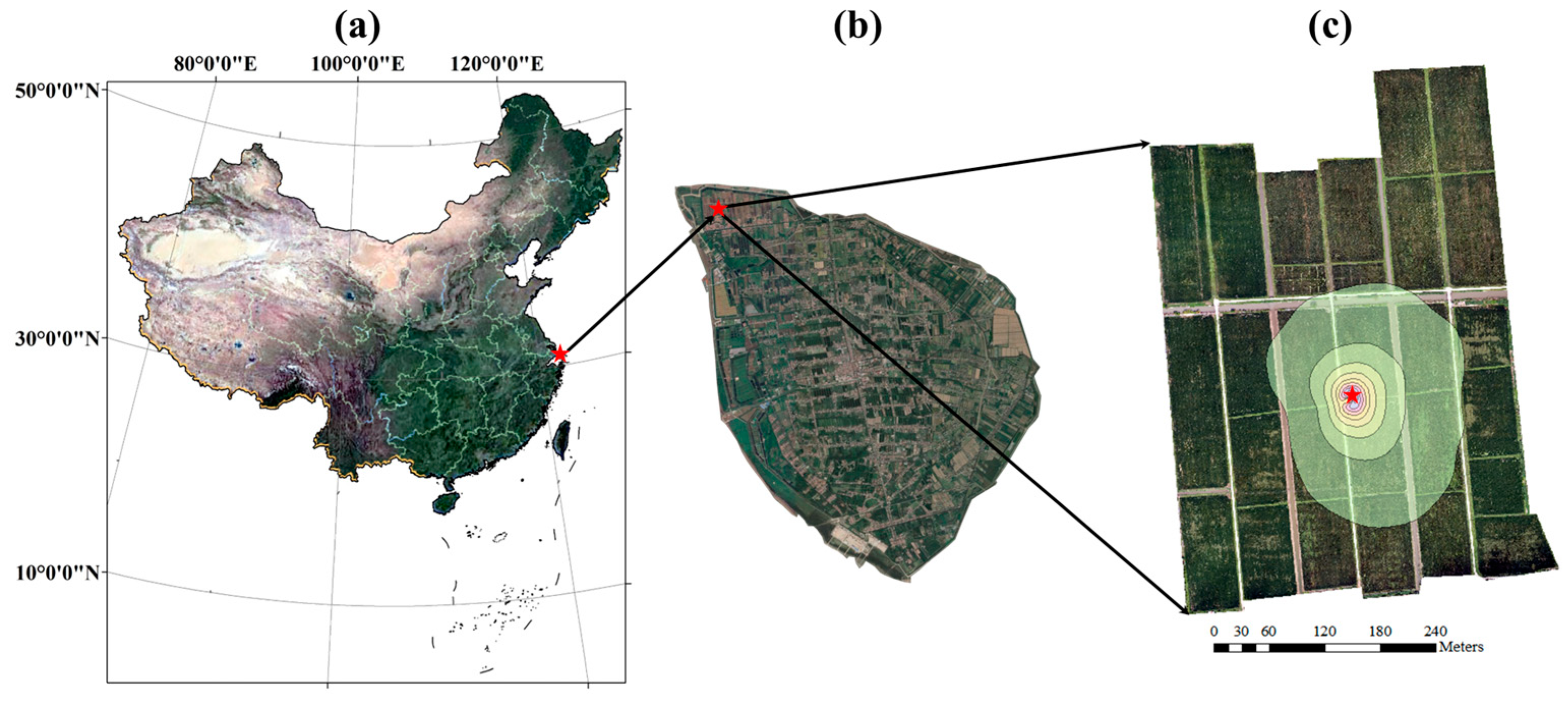
A two-year experiment from 2022 to 2023 was conducted in an 18.93 ha paddy field, located in Hengsha Country, Shanghai City, China (Figure 2). Rice was transplanted on June 1st, 2022, and May 25th, 2023, and harvested on December 3rd, 2022, and October 20th, 2023. The soil texture was silt loam, with a mean dry bulk density of 1.37 g cm−3 and a mean saturated volumetric soil water content of 44.23%. The paddy field maintained a water layer with a 5–20 cm depth, except during the late tillering and full ripening stages. The plant density was 2.38 × 10⁵ plants ha−1.

Figure 2.
The location of the experiment site. The red five-pointed star represents the EC system. The contour lines of the footprint during the growing period in (3) are shown in steps of 10% from 10 to 90%. The background maps in (a,b) are RGB images from Google Earth. The background map in (c) is the RGB image from the UAV platform.
2.1.1. Eddy Flux and Micrometeorological Measurements
The eddy covariance system (IRGASON, Campbell Scientific, Logan, UT, USA) with an installation height of 2.85 m collected the 10 Hz three-dimensional wind speed and direction, ambient CO2 and H2O density, sonic temperature, and air pressure. The corresponding meteorological and soil elements, including air temperature and humidity (HMP155A, Vaisala Ojy, Vantaa, Finland), incoming outgoing shortwave radiations (CNR4-L, Kipp & Zonen, Delft, The Netherlands), four-layer soil moisture, and temperature at 5 cm, 10 cm, 20 cm, and 40 cm (TDR310N, Acclima, Meridian, ID, USA) were measured.
The 30 min eddy fluxes, including net ecosystem exchange (NEE), latent heat flux (LE), sensible heat flux (H), and friction velocity (u*), were generated from 10 Hz raw data of the EC system using the EddyPro software v7.0.9 (www.licor.com/). The data quality of eddy flux was evaluated using the scheme proposed by Foken et al. [43], which classifies the flux data into 9 levels. The data labeled as levels 7–9 were regarded as low-quality and removed. In addition, the flux data were dropped when u* was less than a specific threshold that indicated the period of low turbulent mixing. The u* threshold was calculated for each season using the moving point method [43]. The seasonal u* threshold is shown in Table S1 (see Supplementary Material Section S2). Then, the missing flux data were filled using the marginal distribution sampling method [44]. Finally, the 30 min NEE observation was partitioned into GPP and ecosystem respiration (Reco) using the night-time flux partitioning method [44]. The processes of u* filter, gap filling, and flux partitioning were conducted using the REddyProc package [45].
To determine the spatial extent of the EC system measurement, the flux footprint was calculated using the Kljun model [46], which requires the standard deviation of lateral velocity fluctuations (σy), friction velocity (u*), Obukhov length (L), wind speed (u), and boundary layer height (blh) (see Supplementary Material, Section S2). σy, u*, L, and u were measured from the EC system. There was no direct measurement of blh, so we adopted the blh data from ERA5 hourly data on singe-level products (https://cds.climate.copernicus.eu/datasets/reanalysis-era5-single-levels, accessed on 17 October 2024) in this study. Then, an 80% footprint was regarded as the measurement range of the EC system.
2.1.2. UAV Data Collection
RGB and multispectral images were acquired using DJI Phantom 4 Multispectral (P4M) (SZ DJI Technology Co., Ltd., Shenzhen, China), equipped with one RGB sensor and five monochrome sensors to measure spectral response in the blue (450 nm ± 16 nm), green (560 nm ± 16 nm), red (650 nm ± 16 nm), red-edge (730 nm ± 16 nm) and nir (840 nm ± 16 nm) bands. Flight operations were conducted between 9:00 AM and 12:00 AM at an altitude of 120 m. The Pix4dMapper software v4.4.9 was employed to process the raw photos captured by UAV to generate the RGB orthomosaics and reflectance maps with a spatial resolution of 6.5 cm/pixel. The reflectance maps underwent correction using the images of the calibrated reflectance panel (MicaSense, RP06), which were captured during the UAV flight. Georeferencing was performed using ArcGIS software v10.8.2 to ensure pixel alignment in the UAV images. In total, 33 UAV observations were collected (Table 1). To build the daily model, the daily UAV images were generated using linear interpolation for each pixel. Then, daily UAV images were clipped using the external rectangle of the flux footprint climatology during the rice growth season and masked using daily flux footprint climatology (see Supplementary Material, Section S3).

Table 1.
The date of the UAV flight.
2.1.3. Canopy Parameters and Canopy Height Measurement
The plant area index (PAI) and clumping index (Ω) were measured using an LI-COR 2200 canopy analyzer. The leaf area index (LAI) was extracted from the PAI using an empirical method proposed by [47] (see Supplementary Material Section S4). Canopy height (hc) was measured using a tape measure. PAI, Ω and hc were all measured at fixed positions in the paddy field. There were 39 sampling positions in 2022 and 30 in 2023, respectively.
2.2. Leaf Biochemical Properties-Based Model
In this study, we employed the Boreal Ecosystem Productivity Simulator (BEPS) [48] for half-hourly GPP estimations. The BEPS model is based on leaf biochemical properties and follows a two-leaf scheme, which separated the canopy into sunlit leaves and shaded leaves using the following methods:
where θ is the solar zenith angle; Ω is the clumping index; LAI, LAIsunlit, and LAIshaded are the total leaf area index of the canopy, leaf area index of sunlit leaves, and leaf area index of shaded leaves, respectively.
The BEPS model calculates the instantaneous GPP as the sum of photosynthesis from the sunlit leaves and shaded leaves.
where Asunlit and Ashaded are the instantaneous photosynthesis rates of the representative sunlit leaf and representative shaded leaf (μmol m−2 s−1), respectively. The instantaneous photosynthesis rate is calculated using the Farquhar–von Caemmerer–Berry (FvCB) biochemical model [7].
where Wc is the RuBP carboxylation rate limited by Rubisco activity (μmol m−2 s−1); Wj is the RuBP carboxylation rate limited by electron transport (μmol m−2 s−1); Rd is the leaf dark respiration during the daytime (μmol m−2 s−1).
where Ci is the CO2 concentration in the intercellular air space (μmol mol−1); O is the O2 concentration in the intercellular air space and is set as 210 (mmol mol−1); Kc is the Michaelis–Menten constant of Rubisco for CO2 (μmol mol−1); Ko is the Michaelis–Menten constant of Rubisco for O2 (mmol mol−1); Γ* is the CO2 compensation point in the absence of leaf dark respiration (μmol mol−1); J is the electron transport rate (μmol e− m−2 s−1), and is a function of the incoming photon flux density (PPFD, μmol photon m−2 s−1) and Jmax:
The temperature dependence of Ko, Kc, Γ* is described using the Arrhenius function [49]:
The temperature dependence of Vcmax and Jmax is described using the modified Arrhenius function [49]:
where k25 is the parameter value at 25 °C; Tl is the leaf temperature (°C); R is the universal gas constant (8.314 J K−1 mol−1); Ea is the activation energy (J mol−1); Hd is the deactivation energy (J mol−1); ΔS is the entropy term (J K−1 mol−1).
The classical BEPS model assumes that a linear relationship exists between the maximum carboxylation rate and leaf nitrogen content, and leaf nitrogen decreases exponentially from top to bottom in a canopy [48]. In this study, we assumed that the maximum carboxylation rate decreases exponentially from top to bottom in the canopy and eliminated the two parameters, namely nitrogen content at the top of the canopy and the relative change in with leaf nitrogen content.
Therefore, the of representative sunlit and shaded leaves are calculated as follows (see the Supplementary Material Section S5):
where is the at the top of the canopy (μmol m−2 s−1); kn is the leaf nitrogen content decay rate with increasing depth into the canopy and is taken as 0.3; k = G(θ)Ω/cosθ, and the projection coefficient G(θ) is taken as 0.5 for the assumption of spherical leaf angle distribution. The maximum electron transport rate for the sunlit and shaded leaves (Jmax, sunlit, Jmax,shaded, μmol m−2 s−1) is obtained using the following equation [50]:
The leaf stomatal conductance for CO2 (gsc) is coupled with photosynthesis using the Ball–Woodrow–Berry equation [51]:
where hs is the relative humidity at the leaf surface (%); Cs is the CO2 concentration at the leaf surface (μmol mol−1); m and b are the coefficients in the Ball–Woodrow–Berry equation, respectively. m and b are set as 6.08 and 0.019, respectively. These two values were obtained by fitting steady-state-condition A-Ci curves from Li-6800. More detailed information on the BEPS model can be found in the Supplementary Material, Section S6. The BEPS model also considers the influence of soil water stress on gs [48]. Given that rice cultivation typically involves a flooded or saturated state, with minimal exposure to soil water stress, the impact of the soil water stress factor on gs was not considered in this study.
2.3. Derivation of Field-Scale Measurement
This study employed a classical optimization algorithm, the differential evolution (DE) algorithm [52], to retrieve the daily . The differential evolution algorithm contains three steps, including mutation, crossover, and selection. Detailed information about DE algorithm were displayed in the Supplementary Material Section S7. The differential evolution algorithm was implemented using the lmfit python package [53], with the mean square error (MSE) chosen as the objective function. Integrating the DE algorithm with BEPS, called BEPS-DE framework, was employed to derive the field-scale under the assumption of constant for 7 days. Only daytime GPP observation (when incoming shortwave radiation is larger than 0) were used to fit because the BEPS model sets nigh-time GPP as 0 while night-time GPP observation from the EC system are not 0.
2.4. Texture Extraction and Models
In this study, several types of texture features were evaluated for field-scale estimation.
2.4.1. Standard Deviation Texture
The first texture feature is the standard deviation of reflectance within the flux footprint climatology.
where xi is the reflectance value at each pixel within the flux footprint climatology; is the mean reflectance value within the footprint climatology.
2.4.2. GLCM-Based Texture Features
GLCM is a square matrix that can examine the spatial distribution of the gray levels in the image. It describes how frequently a combination of pixels is present in an image in a given direction and distance. For a given image I with a size of K×K and maximum gray value of G, the element of a GLCM for a displacement vector d(dx, dy) is defined as follows:
where dx = dcosθ; dy = dsinθ; d and θ are the predefined distance and direction, respectively. The GLCM is typically interpreted using texture indicators. Six GLCM-based texture features (Table 2) were extracted from UAV images.

Table 2.
The list of GLCM-based texture features in this study.
The computation of GLCM is influenced by the pixel pair distance offsets and pixel pair angles. We pre-specified a series of distance offsets (1,2,4,8,16) and angles (0, π/4, π/2, 3π/4). Then, 20 GLCMs, each representing a unique combination of distance offsets and angles, were employed to derive texture samples. Finally, the mean of 20 texture samples was set as the texture feature of the image.
2.4.3. LBP Texture
The LBP represents each image pixel with a local binary pattern operator that generates a binary code while comparing a neighboring pixel and its center patch gray unit. The LBP codes are computed as follows:
where qc is the gray value of the center pixel; qp is the gray value of P neighboring pixels with a specified radius R. The LBP is invariant against any monotonic transformation of image brightness. The local binary pattern histogram (LBPH) is a commonly used LBP-type texture feature. It employs the distribution of the LBP value to represent the image. A whole image is typically divided into several local regions, and the histograms from each subregion are extracted independently. Then, these subregional histograms are concatenated to build a global description. In this study, we divided the UAV images into 9 subregions (3 × 3), calculated the histogram with 10 bins, and then concatenated the 9 histograms together to obtain the LBPH texture with 90 features. Figure S3 shows the process of extracting the LBPH texture.
2.4.4. Convolutional Neural Network
In this study, we adopted two typically convolutional neural network architectures, including AlexNet [38] and ResNet [54], to extract spatial information from UAV images. ResNet is more complex and has a deeper structure than AlexNet (Figure S4). It is important to note that the input images should maintain the same size when fed into the CNN. Since images with a resolution of 6.5 cm/pixel are too large for the CNN to handle efficiently, UAV images were resampled to a 1m resolution and clipped by the external rectangle (see Section 2.1.2) to maintain the same size. Pixels outside the flux footprint climatology were set as 0. The five-band multispectral images were concatenated into an input tensor (430 × 420 × 5). The input images were preprocessed using the standardization and then fed into the CNN to estimate field-scale .
The different combinations of texture features for were evaluated (Table 3). For the mean and standard deviation of the 5-band reflectance, GLCM-based texture features, and LBPH-driven models, the deep neural network (DNN) was employed to estimate field-scale .
where x is the input layer, namely the combination of the 5-band reflectance and corresponding texture features; hl is the l-th hidden layer; wl and bl are the weights and bias of the l-th layer; fl is the activation function of the l-th layer. The performance of the deep neural network highly relies on hyperparameters, including the number of hidden layers, the number of neurons, the selection of activation function, and the dropout value. We used the genetic programming algorithm to optimize the hyperparameters. The search space was set as follows: (1) the maximum number of hidden layer was set as 4; (2) the number of neurons for each hidden layer was selected from the set [16,32,64,128,256,512,1024]; (3) the activation function for each hidden layer was selected as either ReLU or sigmoid; (4) the dropout rate for each hidden layer was selected from an interval of 0 to 0.5. The daily and corresponding multispectral surface reflectance for each land cover type were randomly apportioned into training and validation sets, with an 80–20 split. The former was used to train the weights and biases, and the latter was employed to evaluate the generalization error.

Table 3.
The list of models proposed in this study.
2.5. Feature Contribution Analysis Using the Shaley Value
The Shaley value (SHAP) was adopted to interpret models. In this study. SHAP [55] is a game-theoretic approach to explain the performance of the machine learning model. It can quantify the contribution of the input feature to the prediction for an individual sample. SHAP specifies the explanation using the additive feature attribution method:
where f(x) is the original model, g(x) is the explanation model with simplified input x′; x′∈{0,1}M; x and x′ are related via a mapping function, x=hx(x′); M represents the number of input features; ϕi is the feature attribution for the feature i. The explanation model g has a unique solution:
where |z′| represents the number of non-zero entries in z′, and z′ ⊆ x′; f(x′) = f(hx(z′)) = E[f(z)|zS], and S is the set of non-zero indexes in z′.
3. Results
3.1. Seasonal Variation in Carbon Fluxes, Environmental Elements, and Biophysical Indicators on the Paddy Field
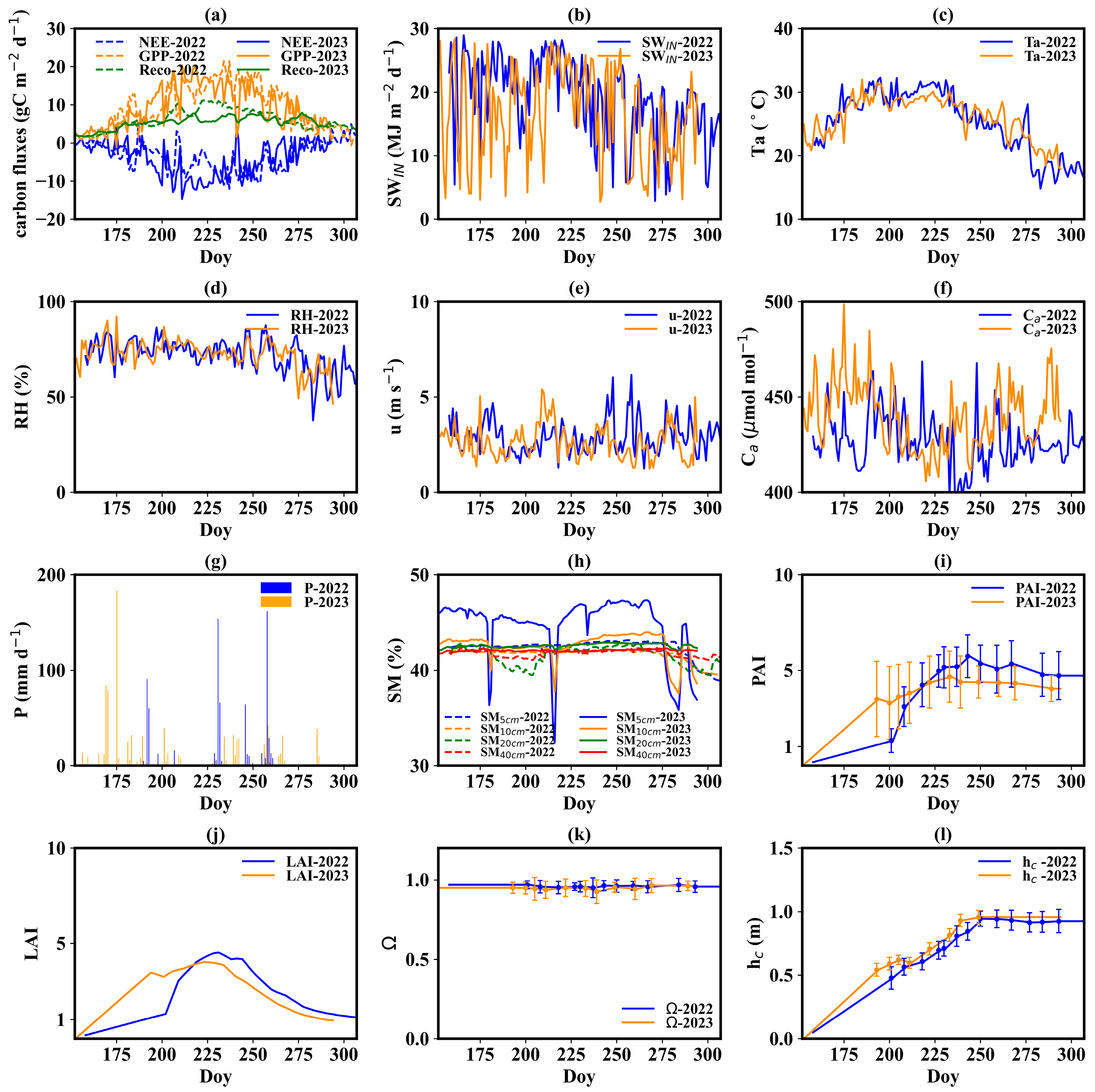
Figure 3a illustrates the seasonal variation in daily NEE, GPP, and Reco during the rice growth period. The NEE displayed a one-valley pattern. The minimum value of daily NEE was −12.08 and −14.60 gC m−2 d−1 in 2022 and 2023, respectively. The two minimum values occurred on August 25th, 2022, and July 29th, 2023. The cumulative NEE in the growth period was 502 and 552 gC m−2. The GPP exhibited a one-peak mode, with peak daily values of 21.6 and 20.16 gC m−2 d−1 in 2022 and 2023, respectively. The peak value occurred on August 21st, 2022, and July 29th, 2023. Total GPP during the growth period was 1429 gC m−2 in 2022 and 1337 gC m−2 in 2023. A strong fluctuation can be found in the dynamics of NEE and GPP, while daily Reco changed smoothly.
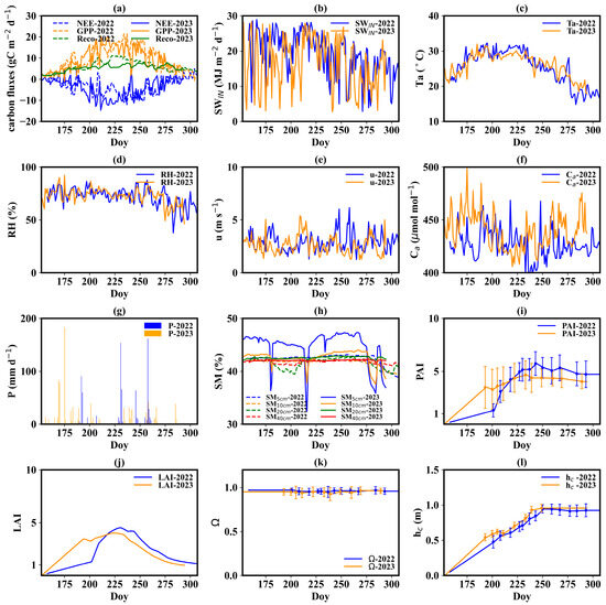
Figure 3.
Seasonal variation in daily carbon fluxes, environmental elements and biophysical indicators. (a) Carbon fluxes, including net ecosystem exchange, gross primary production, and ecosystem respiration; (b) incoming shortwave radiation; (c) air temperature; (d) humidity; (e) wind speed; (f) ambient CO2 concentration; (g) precipitation; (h) soil moisture; (i) plant area index; (j) leaf area index; (k) clumping index; (l) canopy height. The term ‘Doy’ means day of the year.
The summer of 2022 witnessed a severe meteorological drought along the Yangtze River. Accordingly, the incoming shortwave radiation (SWIN) and air temperature (Ta) in 2022 were significantly higher than those in 2023 (Figure 3b,c). The daily mean SWIN and Ta during the summer of 2022 were 21.35 MJ m−2 d−1 and 28.4 °C. The two values at the same time in 2023 were 18.00 MJ m−2 d−1 and 27.1 °C. The difference in Ta on the same days between 2022 and 2023 during the summer was as large as 6 °C. Moreover, 2022 experienced lower precipitation (P) and relative humidity (RH) compared to 2023, with mean RH values of 71% and 76, and accumulated P values of 759 and 922 mm during the growth period for 2022 and 2023, respectively (Figure 3d,g). Precipitation was more frequent in 2023, particularly during the summer. Differences in wind speed (u) and atmospheric CO₂ concentration (Ca) between the two years were minimal (Figure 3e,f), with wind speeds of 2.93 m s−1 in 2022 and 2.62 m s−1 in 2023, and CO₂ concentrations of 426 μmol mol−1 in 2022 and 439 μmol mol−1 in 2023. Due to the presence of a persistent water layer in the paddy field and a shallow groundwater table (about 0.5 m), only surface soil moisture (SM) went through several drying processes, while deep SM remained stable (Figure 3h). Therefore, rice rarely suffered soil water stress during the growth period.
When it comes to biophysical indicators, both PAI and hc reached the plateau at the end of August (at the early heading and flowering stage) (Figure 3i,l). LAI also reached its peak at the end of August with a peak value of 4.52 and 4.03 in 2022 and 2023, respectively (Figure 3j). Then, LAI gradually declined due to leaf senescence. The PAI in 2022 was higher than that in 2023. The former reached 5.84 and the latter 4.44. The gap between 2022 and 2023 hc values was small. The maximum hc was about 0.95 m. The dynamics of Ω were stable during the growth period, with values varying from 0.93 to 0.96 (Figure 3k).
3.2. Seasonal Variation of Observation
Figure 4 presents the seasonal dynamics of field-scale . The field-scale generally presented a single-peak pattern during the growth period, reaching its maximum in mid-July and declining after mid-August. The peak field-scale was approximately 170 μmol m−2 s−1. There were two significant drops in field-scale in early July and in the end of July in 2022, likely due to weed removal activities. In 2022, weed prevention before rice sowing was ineffective, leading to the thriving of weeds. Consequently, a substantial portion of the carbon flux in the paddy field came from the contribution of weeds.
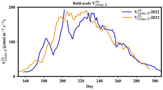
Figure 4.
Seasonal variation in field-scale .
3.3. Accuracy of and GPP Estimation
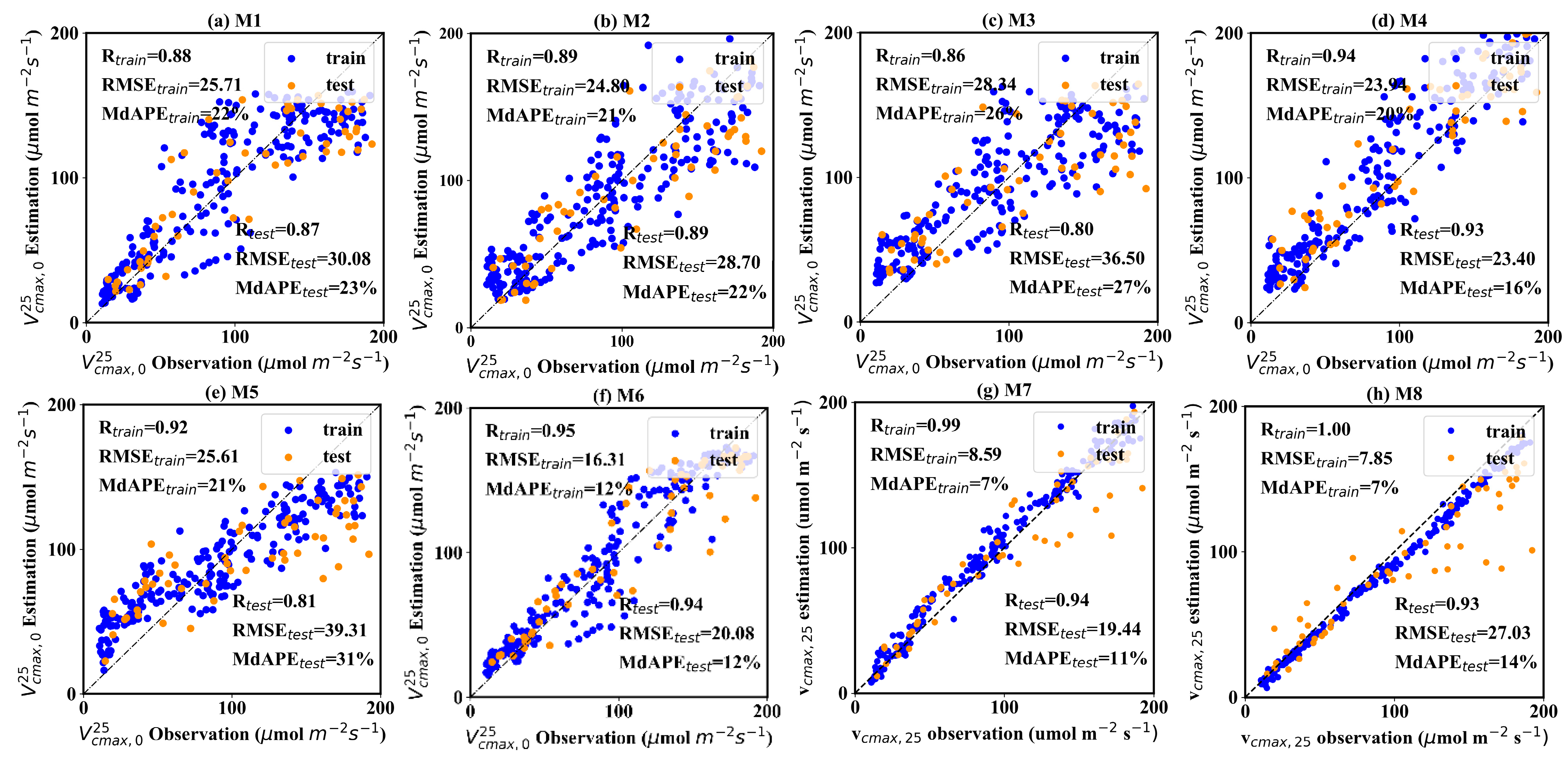
Figure 5 shows the performance of eight models. Three metrics, including correlation (R), root mean square error (RMSE), and medium absolute percentage error (MdAPE), were employed to assess the model performance. When employing traditional reflectance values as input (Figure 5a), the R, RMSE, and MdAPE of estimation on the test dataset were 0.87, 30.08 μmol m−2 s−1 and 23%, respectively. In contrast, the model driven solely by texture information displayed a noticeable performance degradation. The GLCM texture-driven model achieved estimation with an R of 0.80, RMSE of 36.50 μmol m−2 s−1 and MdAPE of 27% on the test dataset (Figure 5c). The LBPH-driven model exhibited the poorest accuracy, with R, RMSE, and MdAPE values of 0.81, 39.31, and 31% on the test dataset, respectively (Figure 5e). However, it can be seen that combining the reflectance value and texture information can significantly improve the accuracy of estimation, while the contribution of differing texture information varies significantly. Two joint-driven models, including μref -GLCM texture feature and μref-LBPH texture feature models, substantially improved the estimations, with R values reaching 0.93–0.94, and RMSE and MdAPE falling from 20.08 to 23.40 μmol m−2 s−1 and 12% to 16%, respectively. However, the combination of μref and σref provided only a marginal improvement, with an R of 0.89, RMSE of 28.70 μmol m−2 s−1 and MdAPE of 22% (Figure 5b). Two CNN methods demonstrated excellent performance. ResNet is typically superior to AlexNet in the ImageNet classification challenge, whereas AlexNet slightly outperformed ResNet in this study. The former acquired the estimation with an R of 0.94, RMSE of 23.70 μmol m−2 s−1, and MdAPE of 11%. The latter obtained the estimation with an R of 0.93, RMSE of 27.30 μmol m−2 s−1, and MdAPE of 14%. A noteworthy observation is that the CNN methods showed an overwhelming advantage over other models on the training dataset, with R reaching 1, and RMSE and MdAPE being lower than 10 μmol m−2 s−1 and 10%. Although this result indicates that the CNN methods encountered a degree of overfitting, it still suggests a strong ability to discern and utilize spatial information embedded in UAV images. The ResNet, with a more complicated structure, displays significantly higher potential than the AlexNet. The overfitting issue of CNN methods can be alleviated by training with more data. As the dataset expands, there is a promising outlook for CNN methods to transcend these challenges and realize significant success.
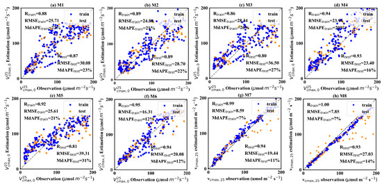
Figure 5.
The accuracy of 8 field-scale models. The blue points represent the training samples, and the orange points represent the validation samples. The sample numbers of the training and validation dataset are 224 and 57, respectively.
Considering the texture information also contributes to the GPP estimation, it can be found that the superior models result in more accurate GPP estimation (Figure 6). Two CNN models acquired the best GPP estimation, with an R of 0.92, RMSE of 6.5–6.6 μmol m−2 s−1, and MdAPE of 23–24%. The uref -GLCM texture feature and the uref -LBPH texture feature joint-driven models also achieved excellent GPP estimation. The former obtained the lowest RMSE, with a value of 6.43 μmol m−2 s−1. The latter also obtained promising results, with an R of 0.92, RMSE of 6.74 μmol m−2 s−1, and MdAPE of 26%. The μref-σref joint-driven model and LBPH solely driven model performed worst for GPP estimation. The RMSE of the two models was larger than 7 μmol m−2, and the MdAPE was over 30%. The μref-GLCM-based texture feature joint-driven model achieved better performance in estimation in the high- range (Figure 5d). In contrast, the two CNN models showed an obvious underestimation issue when was high (Figure 5g–h), and the underestimation of further resulted in a significant bias for high GPP estimation.
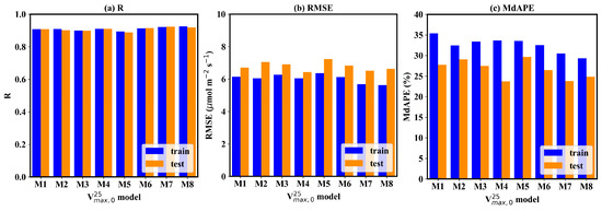
Figure 6.
The accuracy of GPP estimation based on the 8 field-scale models. The blue bar represents the accuracy metrics on the training dataset, and the orange bar represents the accuracy metrics on the testing dataset.
4. Discussion
4.1. How Spatial Information Contributes to Field-Scale Estimation
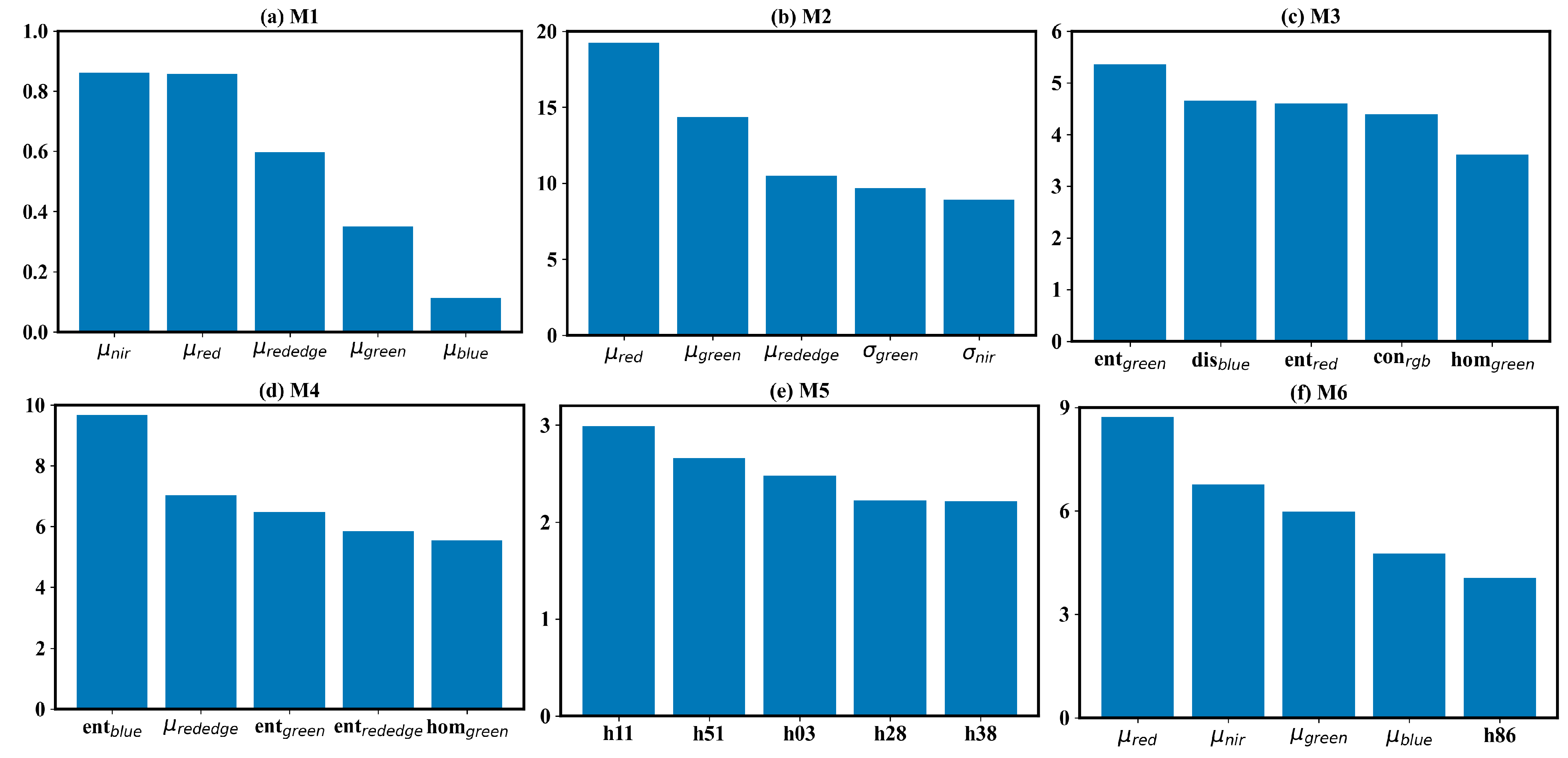
This study assessed different forms of texture information for field-scale estimation and revealed significant differences in the ability of different texture features to describe field-scale . We further elucidated the contribution of differing texture information using the SHAP method. Figure 7 shows the mean of the absolute SHAP (mean(|SHAP|)) for the six deep neural network-based models. Due to the high dimensionality of input data, only the top five most important features were presented. In the μref-driven model (Figure 7a), the nir and red bands contributed most. This result is consistent with the current understanding of the relationship between and the spectrum. These two bands indicate the vegetation growth information and are the components of some classical vegetation indices, such as NDVI and EVI. In the GLCM-based texture-feature-driven- model (Figure 7c), the top 5 most important features were entropy in the green and red bands, dissimilarity in the blue band, contrast in the RGB band, and homogeneity in the green band. The five features exhibited nearly equal importance. In the LBPH-driven model (Figure 7e), the top five most important features were the histogram bars from subregions 1, 5, 1, 2, 3. In the μref-σref joint-driven model (Figure 7b), the top 5 most important features included mean value in red, green, and red-edge bands, and the standard deviation value in the green and nir bands. Here, the mean value information played a dominant role, and the standard deviation information played a subordinate one. Adding the standard deviation information diminished the importance of the nir band, which contributed most in the μref -driven model. In the μref-GLCM-based texture feature joint-driven model, the GLCM-based texture features contributed more than the mean reflectance. There were four GLCM textures in the top five most important features, including entropy in the blue, green and red-edge bands, and homogeneity. Conversely, the mean reflectance played a dominant role in the μref-LBPH joint-driven model. The mean values of reflectance in the red, nir, green and blue bands were the top four most important features in this model. The most important LBPH feature was the histogram bar in subregion 8. The SHAP-based feature importance analysis suggests that entropy is a valuable feature for estimation, with dissimilarity and homogeneity also showing potential. The entropy, dissimilarity, and homogeneity describe the uncertainty of, local variation in, and smoothness of the image texture, respectively [56]. There perhaps exists some inherent link between and these GLCM-based texture features. While standard deviation is a simple and intuitive indicator of spatial heterogeneity, it offered limited information for estimation. The LBPH also failed to indicate the dynamics of . Although this method is regarded as a powerful tool for describing local information and has achieved success in classification issues such as face recognition and weed detection, the histogram-format texture descriptor may be unsuitable for regression issues. LBPH failed to provide stable features for quantifying . Despite this, the combination creating the μref-LBPH joint-driven model outperforms the other two μref-texture joint-driven model. A possible reason is that LBPH is a high-dimensional feature and contains more potential information. In summary, textures are important but may be better used as Supplementary Information to estimate field-scale .

Figure 7.
SHAP-based feature importance analysis for the DNN model. The feature importance is defined as the mean of the absolute value of the SHAP for each feature (mean(|SHAP|)). Only the top 5 most important features are displayed.
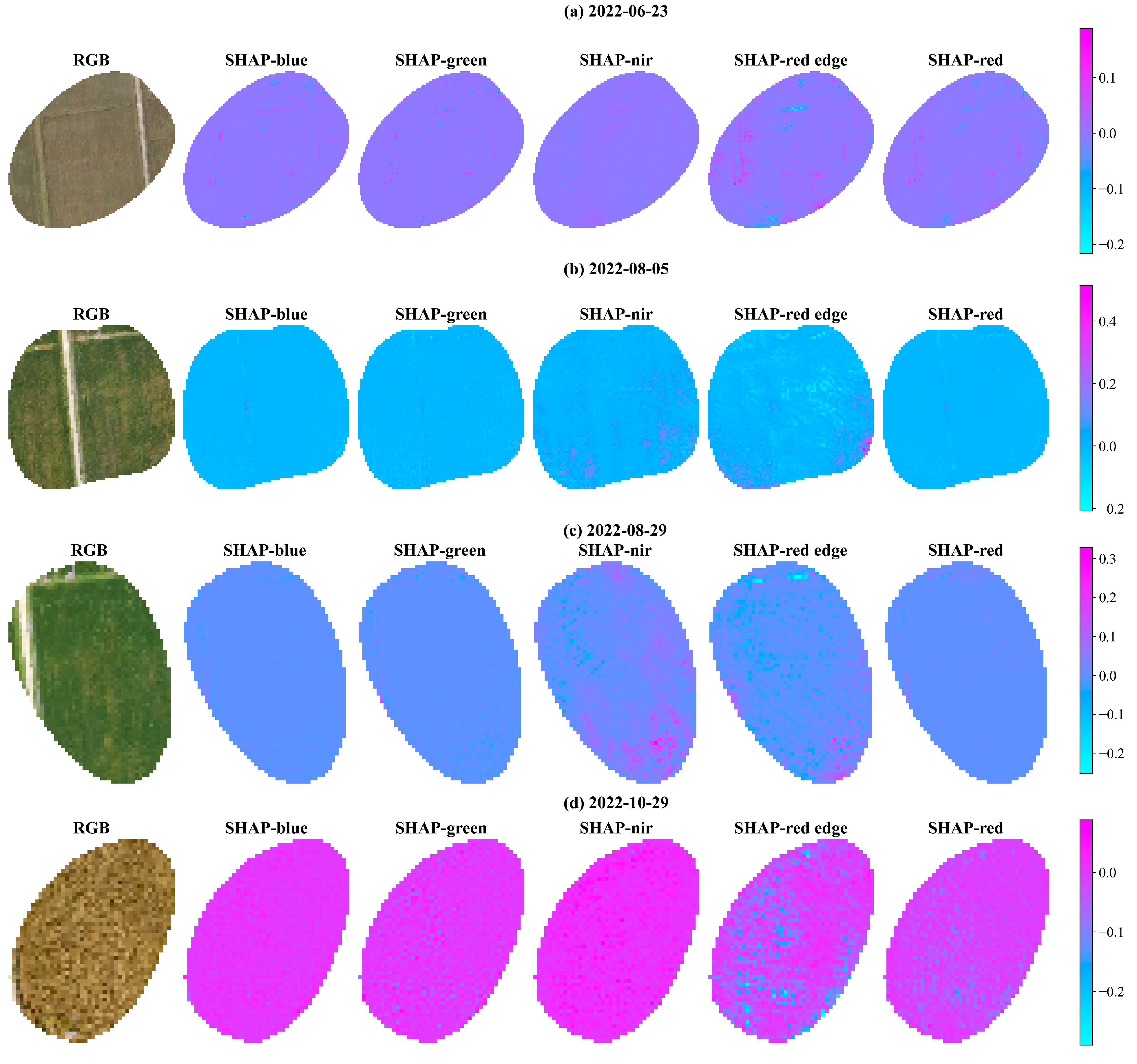
The SHAP method was also employed to interpret the AlexNet-based . Figure 8 shows the spatial distribution of SHAP on 4 typical days, clearly revealing the spatial heterogeneity in the SHAP maps. The contributions from roadway and water bodies differed obviously from those from the paddy field. When the underlying surface was bare soil, the spatial variability in SHAPs across bands was relatively low. When the paddy field was covered by rice, the SHAP variability intensified, particularly in the nir and red-edge bands. Specifically, the regions with a high contribution in these bands were closely linked to areas with a mix of vegetation and bare soil or blends of well-growing and poor-growing vegetation. As the rice matured, the spatial variability in the SHAP in the nir band weakened, while its variability in the red band intensified. To sum up, the CNN model attached much importance to the subregion with high spatial heterogeneity in the nir and red-edge bands for estimation. This emphasis was particularly evident in regions characterized by a mix of vegetation and bare soil, and a mix of well-growing and poor-growing vegetation. The SHAP method was not used to analyze the ResNet-based model due to the complexity of ResNet, which made SHAP computation too resource-intensive. Therefore, the feature contribution of the ResNet-based model was not included in this study.
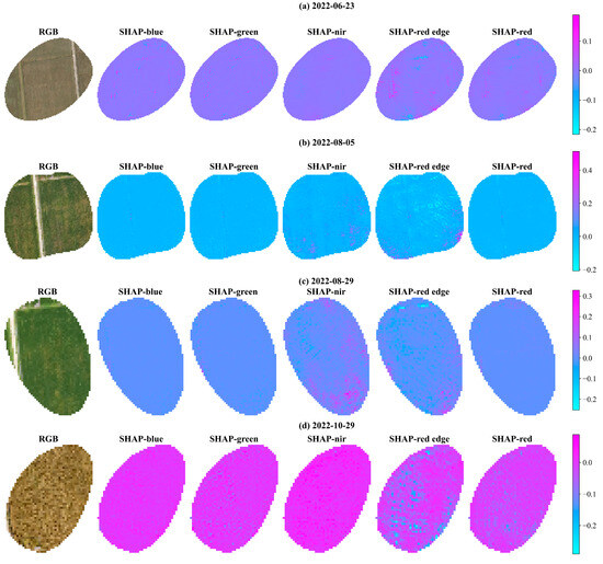
Figure 8.
The spatial distribution of the AlexNet-model-based SHAP.
It should be noted that UAV images were resampled from 6.5 cm/pixel to 1 m/pixel before being fed into the CNN due to limitations to computation capacity. Resampling large images to a smaller, manageable resolution is the most common approach, and this was employed in this study. This approach retains the global spatial information but loses the fine-scale features. The loss of spatial detail will possibly affect the extraction of textural features. Alternative strategies, such as patch-based processing [57], and patch gradient descent [58], offer promising solutions to these challenges. Developing comprehensive methods to interpret ultra-high-resolution UAV images using deep learning is a key area for future exploration.
4.2. Spatial Heterogeneity: Implications for Parameters Conversion Across Different Scales
Our study underscores the significant influence of spatial heterogeneity field-scale . The spatial heterogeneity originates from the diverse elements in paddy fields, including the bare soil, water body, and weeds, as well as rice in different growth states, all of which have distinct photosynthetic properties. Field-scale , representing a macroscopic feature within the flux footprint climatology, is intricately linked to this spatial heterogeneity. In contrast, leaf-scale solely reflects the local feature. This inherent spatial heterogeneity contributes to the observed mismatch between field-scale and leaf-scale , as depicted in Figure S6 (see Supplementary Material Section S11). Given the global prevalence of spatial heterogeneity, as evidenced in various studies [59], relying solely on the leaf-scale model for field-scale simulation introduces uncertainties into GPP estimation. Our study advocates for the direct use of field-scale parameters to model GPP, acknowledging the complexities introduced by spatial heterogeneity.
4.3. Limitations
In this study, we proposed high-resolution UAV-image-based models for field-scale and GPP estimation and demonstrated enhancement through texture information. However, some limitations remain. Firstly, the field-scale observation was retrieved from the BEPS-DE framework. The accuracy of observation was completely determined by the EC-based GPP observation and the structure of the BEPS model. We note that there are several different methods for conducting observation, including the data assimilation approach, sunlit GPP-based inverting method [60], and optimality photosynthesis hypothesis-based approach [15]. In addition, the BEPS model is highly parameterized, with many parameters predefined. The uncertainties in these predefined parameters will ultimately influence the retrieval of . For example, Jiang et al. [61] revealed that the variation in the nitrogen distribution coefficient within the canopy (kn) resulted in a large gap between retrieved values. Therefore, it is necessary to comprehensively evaluate the different retrieval methods. This study evaluates four typical spatial information extraction methods, including σref, GLCM texture, LBPH texture, and CNN. Some newly proposed texture features, such as learning-based approaches and the entropy-based approaches, have garnered significant attention [28]. It is necessary to explore the capabilities of these new features for GPP estimation. Lastly, this study faced some challenges in sample size. The overwhelming advantage of CNN models in the training dataset demonstrates its strong ability to extract valuable spatial information. The performance of CNN algorithms primarily depends on big training data. The CNN-based models were trained and validated only using 281 daily RBG and five-band reflectance maps. Compared with the complex structure of the CNN, the sample size in this study is relatively insufficient, resulting in a degree of overfitting. It is urgent to expand our dataset to fully harness the potential of deep learning.
5. Conclusions
Accurate estimation of GPP estimation poses a considerable challenge due to the influence of spatial heterogeneity. High-resolution UAV images can capture spatial heterogeneity and offer new insights for GPP monitoring. In this study, we proposed high-resolution UAV-imagery-driven models to quantify , a key parameter of the leaf biochemical properties-based GPP model. The reflectance and texture information were extracted from UAV images and employed to build models. A significant improvement in and GPP estimation was obtained. The main conclusions are drawn as follows:
- (1)
- Combining reflectance and texture features can vastly improve the field-scale (R = 0.94, RMSE = 19.44 μmol m−2 s−1, and MdAPE = 11%) and further result in high-accuracy GPP estimation (R = 0.92, RMSE = 6.5 μmol m−2 s−1, and MdAPE = 23%). The performance of different texture features varies significantly. The CNN method shows the strongest ability to monitor . The μref-GLCM texture features and μref-LBPH joint-driven models also acquire promising results. However, the standard deviation of reflectance contributes less to estimating .
- (2)
- The contribution of input features changes significantly among different models. The CNN model focuses on nir and red-edge bands and pays much attention to the subregion with high spatial heterogeneity. The μref-LBPH joint-driven model mainly attaches importance to the reflectance information. On the other hand, the μref-GLCM-based features joint-driven model emphasizes the role of GLCM texture indices, including contrast, dissimilarity and homogeneity.
- (3)
- The strong spatial heterogeneity results in the large gap difference between field-scale and leaf-scale values and hinders the conversion of parameters across different scales
Our study confirms the necessity of considering spatial heterogeneity information for monitoring and GPP, which is ignored in the current understanding of the GPP model. The following perspectives should be the focus of future work. First, the fusion of satellite and UAV data offers great potential. Medium-resolution satellites, such as Landsat and Sentinel-2, can capture remote sensing images with spatial resolutions of 10–60 m, providing valuable spatial information about the underlying surface. Additionally, integrating multi-scale remote sensing images can achieve information complementarity, which is likely to enhance the accuracy of GPP monitoring. Second, further exploration of new interpretation methods is needed to better elucidate the mechanistic link between spatial heterogeneity and field-scale parameters.
Supplementary Materials
The following supporting information can be downloaded at https://www.mdpi.com/article/10.3390/rs16203906/s1, Table S1: The seasonal u* threshold for filtering NEE; Table S2: The fixed parameter values in the BESP model; Table S3: The date of leaf gas-exchange experiment; Figure S1: Dynamics of daily RGB and Reflectance maps within the flux footprint climatology; Figure S2: The coefficient of stomatal conductance model; Figure S3: The process of generating LBPH; Figure S4: The architectures of AlexNet and ResNet. The blue block indicates the convolution layer; Figure S5: Dynamics of spatial distribution of SHAP value based on the AlexNet model; Figure S6. Seasonal variation of filed-scale and leaf-scale . References [32,51,62] are cited in the supplementary materials.
Author Contributions
Conceptualization, X.H. and L.S.; methodology, X.H., X.D., J.B. and Z.Z.; software, X.H.; validation, L.L., L.S. and J.B.; formal analysis, X.H.; investigation, X.H.; resources, S.L.; data curation, X.H., X.D., J.L., C.S., S.D., T.W. and Y.W.; writing—original draft preparation, X.H.; writing—review and editing, S.L., L.L. and S.L.; visualization, X.H.; supervision, L.S.; project administration, L.S.; funding acquisition, X.H. and L.L. All authors have read and agreed to the published version of the manuscript.
Funding
This work was funded by the National Natural Science Foundation of China (Grants No. 52309058 and No. U2243235), and the China Postdoctoral Science Foundation 2023M732702.
Data Availability Statement
The data are available from the corresponding author on reasonable request. The data are not publicly available because there are still graduate students using it for research.
Acknowledgments
The authors gratefully acknowledge Shanghai Hengsha Agricultural and Forestry Industrial Development Co., Ltd. for their support in this experiment.
Conflicts of Interest
The authors declare no conflicts of interest.
References
- He, B.; Chen, C.; Lin, S.; Yuan, W.; Chen, H.W.; Chen, D.; Zhang, Y.; Guo, L.; Zhao, X.; Liu, X.; et al. Worldwide impacts of atmospheric vapor pressure deficit on the interannual variability of terrestrial carbon sink. Natl. Sci. Rev. 2022, 9, nwab150. [Google Scholar] [CrossRef] [PubMed]
- Marshall, M.; Tu, K.; Brown, J. Optimizing a remote sensing production efficiency model for macro-scale GPP and yield estimation in agroecosystems. Remote Sens. Environ. 2018, 217, 258–271. [Google Scholar] [CrossRef]
- FAO. World Food and Agriculture-Statistical Yearbook 2022; FAO: Rome, Italy, 2022. [Google Scholar]
- Hwang, Y.; Ryu, Y.; Huang, Y.; Kim, J.; Iwata, H.; Kang, M. Comprehensive assessments of carbon dynamics in an intermittently-irrigated rice paddy. Agric. For. Meteorol. 2020, 285–286, 107933. [Google Scholar] [CrossRef]
- Joiner, J.; Yoshida, Y.; Zhang, Y.; Duveiller, G.; Jung, M.; Lyapustin, A.; Wang, Y.; Tucker, C.J. Estimation of terrestrial global gross primary production (GPP) with satellite data-driven models and eddy covariance flux data. Remote Sens. 2018, 10, 1346. [Google Scholar] [CrossRef]
- Jung, M.; Schwalm, C.; Migliavacca, M.; Walther, S.; Camps-Valls, G.; Koirala, S.; Anthoni, P.; Besnard, S.; Bodesheim, P.; Carvalhais, N.; et al. Scaling carbon fluxes from eddy covariance sites to globe: Synthesis and evaluation of the FLUXCOM approach. Biogeosciences 2020, 17, 1343–1365. [Google Scholar] [CrossRef]
- Farquhar, G.D.; von Caemmerer, S.; Berry, J.A. A biochemical model of photosynthetic CO2 assimilation in leaves of C3 species. Planta 1980, 149, 78–90. [Google Scholar] [CrossRef]
- Collatz, G.; Ribas-Carbo, M.; Berry, J. Coupled Photosynthesis-Stomatal Conductance Model for Leaves of C4Plants. Aust. J. Plant Physiol. 1992, 19, 519. [Google Scholar]
- Chen, J.; Liu, J.; Cihlar, J.; Goulden, M. Daily canopy photosynthesis model through temporal and spatial scaling for remote sensing applications. Ecol. Modell. 1999, 124, 99–119. [Google Scholar] [CrossRef]
- Monteith, J.L. Solar Radiation and Productivity in Tropical Ecosystems. J. Appl. Ecol. 1972, 9, 747. [Google Scholar] [CrossRef]
- Running, S.W.; Nemani, R.R.; Heinsch, F.A.; Zhao, M.; Reeves, M.; Hashimoto, H. A continuous satellite-derived measure of global terrestrial primary production. BioScience 2004, 54, 547. [Google Scholar] [CrossRef]
- Sun, Y.; Frankenberg, C.; Jung, M.; Joiner, J.; Guanter, L.; Köhler, P.; Magney, T. Overview of Solar-Induced chlorophyll Fluorescence (SIF) from the Orbiting Carbon Observatory-2: Retrieval, cross-mission comparison, and global monitoring for GPP. Remote Sens. Environ. 2018, 209, 808–823. [Google Scholar] [CrossRef]
- Campbell, P.K.E.; Huemmrich, K.F.; Middleton, E.M.; Ward, L.A.; Julitta, T.; Daughtry, C.S.T.; Burkart, A.; Russ, A.L.; Kustas, W.P. Diurnal and seasonal variations in chlorophyll fluorescence associated with photosynthesis at leaf and canopy scales. Remote Sens. 2019, 11, 488. [Google Scholar] [CrossRef]
- Luo, X.; Croft, H.; Chen, J.M.; He, L.; Keenan, T.F. Improving estimates of global terrestrial photosynthesis using information on leaf chlorophyll content. Glob. Change Biol. 2019, 25, 2499–2514. [Google Scholar] [CrossRef] [PubMed]
- Smith, N.G.; Keenan, T.F.; Colin Prentice, I.; Wang, H.; Wright, I.J.; Niinemets, Ü.; Crous, K.Y.; Domingues, T.F.; Guerrieri, R.; Zhou, S.X.; et al. Global photosynthetic capacity is optimized to the environment. Ecol. Lett. 2019, 22, 506–517. [Google Scholar] [CrossRef] [PubMed]
- Chen, J.M.; Wang, R.; Liu, Y.; He, L.; Croft, H.; Luo, X.; Wang, H.; Smith, N.G.; Keenan, T.F.; Prentice, I.C.; et al. Global datasets of leaf photosynthetic capacity for ecological and earth system research. Earth Syst. Sci. Data 2022, 14, 4077–4093. [Google Scholar] [CrossRef]
- Evans, J.R. Nitrogen and photosynthesis in the flag leaf of wheat (Triticum aestivum L.). Plant Physiol. 1983, 72, 297–302. [Google Scholar] [CrossRef]
- Ryu, Y.; Baldocchi, D.D.; Kobayashi, H.; Van Ingen, C.; Li, J.; Black, T.A.; Beringer, J.; Van Gorsel, E.; Knohl, A.; Law, B.E.; et al. Integration of MODIS land and atmosphere products with a coupled-process model to estimate gross primary productivity and evapotranspiration from 1 km to global scales. Glob. Biogeochem. Cycles 2011, 25, GB4017. [Google Scholar] [CrossRef]
- Walker, A.P.; Beckerman, A.P.; Gu, L.; Kattge, J.; Cernusak, L.A.; Domingues, T.F.; Woodward, F.I. The relationship of leaf photosynthetic traits—Vcmax and Jmax—to leaf nitrogen, leaf phosphorus, and specific leaf area: A meta-analysis and modeling study. Ecol. Evol. 2014, 4, 3218–3235. [Google Scholar] [CrossRef]
- Croft, H.; Chen, J.; Luo, X.; Bartlett, P.; Chen, B.; Staebler, R. Leaf chlorophyll content as a proxy for leaf photosynthetic capacity. Glob. Change Biol. 2017, 23, 3513–3524. [Google Scholar] [CrossRef]
- Doughty, C.E.; Asner, G.P.; Martin, R.E. Predicting tropical plant physiology from leaf and canopy spectroscopy. Oecologia 2011, 165, 289–299. [Google Scholar] [CrossRef]
- Zhou, Y.; Ju, W.; Sun, X.; Hu, Z.; Han, S.; Black, T.A.; Jassal, R.S.; Wu, X. Close relationship between spectral vegetation indices and Vcmax in deciduous and mixed forests. Tellus B 2014, 66, 23279. [Google Scholar] [CrossRef]
- Zhang, Y.; Guanter, L.; Berry, J.A. Estimation of vegetation photosynthetic capacity from space-based measurements of chlorophyll fluorescence for terrestrial biosphere models. Glob. Change Biol. 2014, 20, 3727–3742. [Google Scholar] [CrossRef] [PubMed]
- Zhang, Y.; Guanter, L.; Joiner, J.; Song, L.; Guan, K. Spatially-explicit monitoring of crop photosynthetic capacity through the use of space-based chlorophyll fluorescence data. Remote Sens. Environ. 2018, 210, 362–374. [Google Scholar] [CrossRef]
- Song, G.; Wang, Q.; Jin, J. Estimation of leaf photosynthetic capacity parameters using spectral indices developed from fractional-order derivatives. Comput. Electron. Agric. 2023, 212, 108068. [Google Scholar] [CrossRef]
- Stoy, P.C.; Mauder, M.; Foken, T.; Marcolla, B.; Boegh, E.; Ibrom, A.; Arain, M.A.; Arneth, A.; Aurela, M.; Bernhofer, C.; et al. A data-driven analysis of energy balance closure across FLUXNET research sites: The role of landscape scale heterogeneity. Agric. For. Meteorol. 2013, 171–172, 137–152. [Google Scholar] [CrossRef]
- Tamura, H.; Mori, S.; Yamawaki, T. Texture features corresponding to visual perception. IEEE Trans. Syst. Man Cybern. 1978, 8, 460–473. [Google Scholar] [CrossRef]
- Humeau-Heurtier, A. Texture feature extraction methods: A survey. IEEE Access 2019, 7, 8975–9000. [Google Scholar] [CrossRef]
- Haralick, R.M.; Shanmugan, K.; Dinstein, I. Texture features for image classification. IEEE Trans. Syst. Man. Cybern. 1973, 3, 610–621. [Google Scholar] [CrossRef]
- Park, Y.; Guldmann, J. Measuring continuous landscape patterns with Gray-Level Co-Occurrence Matrix (GLCM) indices: An alternative to patch metrics? Ecol. Indic. 2020, 109, 105802. [Google Scholar] [CrossRef]
- Fu, Y.; Yang, G.; Song, X.; Li, Z.; Xu, X.; Feng, H.; Zhao, C. Improved estimation of winter wheat aboveground biomass using multiscale textures extracted from UAV-based digital images and hyperspectral feature analysis. Remote Sens. 2021, 13, 581. [Google Scholar] [CrossRef]
- Yang, N.; Zhang, Z.; Zhang, J.; Guo, Y.; Yang, X.; Yu, G.; Bai, X.; Chen, J.; Chen, Y.; Shi, L.; et al. Improving estimation of maize leaf area index by combining of UAV-based multispectral and thermal infrared data: The potential of new texture index. Comput. Electron. Agric. 2023, 214, 108294. [Google Scholar] [CrossRef]
- Reddy, B.S.; Chatterji, B.N. An FFT-based technique for translation, rotation, and scale-invariant image registration. IEEE Trans. Image Process. 1996, 5, 1266–1271. [Google Scholar] [CrossRef] [PubMed]
- Ojala, T.; Pietikäinen, M.; Harwood, D. A comparative study of texture measures with classification based on featured distributions. Pattern Recognit. 1996, 29, 51–59. [Google Scholar] [CrossRef]
- Ahonen, T.; Hadid, A.; Pietikainen, M. Face description with local binary patterns: Application to face recognition. IEEE Trans. Pattern Anal. Mach. Intell. 2006, 28, 2037–2041. [Google Scholar] [CrossRef]
- Duan, B.; Liu, Y.; Gong, Y.; Peng, Y.; Wu, X.; Zhu, R.; Fang, S. Remote estimation of rice LAI based on Fourier spectrum texture from UAV image. Plant Methods 2019, 15, 124. [Google Scholar] [CrossRef]
- Zhuang, J.J.; Luo, S.M.; Hou, C.J.; Tang, Y.; He, Y.; Xue, X.Y. Detection of orchard citrus fruits using a monocular machine vision-based method for automatic fruit picking applications. Comput. Electron. Agric. 2018, 152, 64–73. [Google Scholar] [CrossRef]
- Krizhevsky, A.; Sutskever, I.; Hinton, G.E. ImageNet classification with deep convolutional neural networks. Adv. Neural Inf. Process. Syst. 2012, 25, 1106–1114. [Google Scholar] [CrossRef]
- Yang, Q.; Shi, L.; Han, J.; Zha, Y.; Zhu, P. Deep convolutional neural networks for rice grain yield estimation at the ripening stage using UAV-based remotely sensed images. Field Crops Res. 2019, 235, 142–153. [Google Scholar] [CrossRef]
- Ilniyaz, O.; Du, Q.; Shen, H.; He, W.; Feng, L.; Azadi, H.; Kurban, A.; Chen, X. Leaf area index estimation of pergola-trained vineyards in arid regions using classical and deep learning methods based on UAV-based RGB images. Comput. Electron. Agric. 2023, 207, 107723. [Google Scholar] [CrossRef]
- Sun, S.; Zhu, L.; Liang, N.; He, Y.; Wang, Z.; Chen, S.; Liu, J.; Chen, H.; He, Y.; Zhou, Z. Monitoring drought induced photosynthetic and fluorescent variations of potatoes by visible and thermal imaging analysis. Comput. Electron. Agric. 2023, 215, 108433. [Google Scholar] [CrossRef]
- Deng, X.; Zhang, Z.; Hu, X.; Li, J.; Li, S.; Su, C.; Du, S.; Shi, L. Estimation of photosynthetic parameters from hyperspectral images using optimal deep learning architecture. Comput. Electron. Agric. 2023, 216, 108540. [Google Scholar] [CrossRef]
- Foken, T.; Göckede, M.; Mauder, M.; Mahrt, L.; Amiro, B.; Munger, W. Post-field data quality control. In Handbook of Micrometeorology. A Guide for Surface Flux Measurement and Analysis; Lee, X., Massman, M., Law, B., Eds.; Kluwer Academic: Boston, MA, USA, 2004; pp. 181–208. [Google Scholar]
- Reichstein, M.; Falge, E.; Baldocchi, D.; Papale, D.; Aubinet, M.; Berbigier, P.; Bernhofer, C.; Buchmann, N.; Gilmanov, T.; Granier, A.; et al. On the separation of net ecosystem exchange into assimilation and ecosystem respiration: Review and improved algorithm. Glob. Change Biol. 2005, 11, 1424–1439. [Google Scholar] [CrossRef]
- Wutzler, T.; Lucas-Moffat, A.; Migliavacca, M.; Knauer, J.; Sickel, K.; Šigut, L.; Menzer, O.; Reichstein, M. Basic and extensible post-processing of eddy covariance flux data with REddyProc. Biogeosciences 2018, 15, 5015–5030. [Google Scholar] [CrossRef]
- Kljun, N.; Calanca, P.; Rotach, M.W.; Schmid, H.P. The simple two-dimensional parameterisation for Flux Footprint Predictions FFP. Geosci. Model Dev. 2015, 8, 3695–3713. [Google Scholar] [CrossRef]
- Yang, Q.; Shi, L.; Han, J.; Zha, Y.; Yu, J.; Wu, W.; Huang, K. Regulating the time of the crop model clock: A data assimilation framework for regions with high phenological heterogeneity. Field Crop. Res. 2023, 93, 108847. [Google Scholar] [CrossRef]
- Chen, J.; Mo, G.; Pisek, J.; Liu, J.; Deng, F.; Ishizawa, M.; Cha, D. Effects of foliage clumping on the estimation of global terrestrial gross primary productivity. Glob. Biogeochem. Cycles 2012, 6, GB1019. [Google Scholar] [CrossRef]
- Medlyn, B.E.; Dreyer, E.; Ellsworth, D.; Forstreuter, M.; Harley, P.C.; Kirschbaum, M.U.F.; Roux, X.L.; Montpied, P.; Strassemeyer, J.; Loustau, D.; et al. Temperature response of parameters of a biochemically based model of photosynthesis, I.I. A review of experimental data. Plant Cell Environ. 2002, 25, 1167–1179. [Google Scholar] [CrossRef]
- Medlyn, B.E.; Badeck, F.-W.; De Pury, D.G.G.; Barton, C.V.M.; Broadmeadow, M.; Ceulemans, R.; De Angelis, P.; Forstreuter, M.; Jach, M.E.; Kellomäki, S.; et al. Effects of elevated [CO2] on photosynthesis in European forest species: A meta-analysis of model parameters. Plant Cell Environ. 1999, 22, 1475–1495. [Google Scholar] [CrossRef]
- Ball, M.C.; Woodrow, I.E.; Berry, J.A. A model predicting stomatal conductance and its contribution to the control of photosynthesis under different environmental conditions. In Progress in Photosynthesis Research; Biggins, J., Ed.; Martinus Nijhoff Publishers: Dordrecht, The Netherlands, 1987; pp. 221–224. [Google Scholar]
- Storn, R.; Price, K. Differential evolution—A simple and efficient heuristic for global optimization over continuous spaces. J. Glob. Optim. 1997, 11, 341–359. [Google Scholar] [CrossRef]
- Newville, M.; Stensitzki, T.; Allen, D.B.; Rawlik, M.; Ingargiola, A.; Nelson, A. LMFIT: Non-Linear Least-Square Minimization and Curve-Fitting for Python. Astrophysics Source Code Library: 2016; p. ascl-1606. Available online: https://ui.adsabs.harvard.edu/abs/2016ascl.soft06014N/abstract (accessed on 17 October 2024).
- He, K.; Zhang, X.; Ren, S.; Sun, J. Deep residual learning for image recognition. In Proceedings of the IEEE Conference on Computer Vision and Pattern Recognition, Las Vegas, NV, USA, 27–30 June 2016; pp. 770–778. [Google Scholar]
- Lundberg, S.M.; Lee, S.I. A unified approach to interpreting model predictions. Adv. Neural Inf. Process. Syst. 2017, 30, 4765–4774. [Google Scholar]
- Hlatshwayo, S.T.; Mutanga, O.; Lottering, R.T.; Kiala, Z.; Imsail, R. Mapping forest aboveground biomass in the reforested Buffelsdraai landfill site using texture combinations computed from SPOT-6 pan-sharpened imagery. Int. J. Appl. Earth Obs. Geoinf. 2019, 74, 65–77. [Google Scholar] [CrossRef]
- Zhang, P.; Dai, X.; Yang, J.; Xiao, B.; Yuan, L.; Zhang, L.; Gao, J. Multi-scale vision longformer: A new vision transformer for high-resolution image encoding. In Proceedings of the IEEE/CVF International Conference on Computer Vision, Montreal, QC, Canada, 10–17 October 2021; pp. 2998–3008. [Google Scholar]
- Gupta, D.K.; Mago, G.; Chavan, A.; Prasad, D.K. Patch gradient descent: Training neural networks on very large images. arXiv 2023, arXiv:2301.13817. [Google Scholar]
- Chu, H.; Luo, X.; Ouyang, Z.; Chan, W.S.; Dengel, S.; Biraud, S.C.; Torn, M.S.; Metzger, S.; Kumar, J.; Arain, M.A.; et al. Representativeness of eddy-covariance flux footprints for area surrounding AmeriFlux sites. Agric. For. Meteorol. 2021, 301–302, 108350. [Google Scholar] [CrossRef]
- Zheng, T.; Chen, J.; He, L.; Arain, M.A.; Thomas, S.C.; Murphy, J.G.; Geddes, J.A.; Black, T.A. Inverting the maximum carboxylation rate (Vcmax) from the sunlit leaf photosynthesis rate derived from measured light response curves at tower flux sites. Agric. For. Meteorol. 2017, 236, 48–66. [Google Scholar] [CrossRef]
- Jiang, C.; Ryu, Y.; Wang, H.; Keenan, T.F. An optimality-based model explains seasonal variation in C3 plant photosynthetic capacity. Glob. Change Biol. 2020, 26, 6493–6510. [Google Scholar] [CrossRef]
- Saathoff, A.J.; Welles, J. Gas exchange measurements in the unsteady state. Plant Cell Environ. 2021, 44, 3509–3523. [Google Scholar] [CrossRef]
Disclaimer/Publisher’s Note: The statements, opinions and data contained in all publications are solely those of the individual author(s) and contributor(s) and not of MDPI and/or the editor(s). MDPI and/or the editor(s) disclaim responsibility for any injury to people or property resulting from any ideas, methods, instructions or products referred to in the content. |
© 2024 by the authors. Licensee MDPI, Basel, Switzerland. This article is an open access article distributed under the terms and conditions of the Creative Commons Attribution (CC BY) license (https://creativecommons.org/licenses/by/4.0/).


