Comparative Study of GPR Acquisition Methods for Shallow Buried Object Detection

Abstract

This paper investigates the use of ground-penetrating radar (GPR) technology for detecting shallow buried objects, utilizing an air-coupled stepped frequency continuous wave (SFCW) radar system that operates within a 2 GHz bandwidth starting at 500 MHz. Different GPR data acquisition methods for air-coupled systems are compared, specifically down-looking, side-looking, and circular acquisition strategies, employing the back projection algorithm to provide focusing of the acquired GPR data. Experimental results showed that the GPR can penetrate up to 0.6 m below the surface in a down-looking mode. The developed radar and the back projection focusing algorithm were used to acquire data in the side-looking and circular mode, providing focused images with a resolution of 0.1 m and detecting subsurface objects up to 0.3 m below the surface. The proposed approach transforms B-scans of the GPR-based data into 2D images. The provided approach has significant potential for advancing shallow object detection capabilities by transforming hyperbola-based features into point-like features.

1. Introduction

Over the last decade, ground penetrating radar (GPR) acquisition methods have advanced significantly, driven by technological innovations and expanded applications. Enhanced hardware components, such as improved antenna designs and higher-frequency ranges, have increased resolution and depth penetration, enabling more precise surface and subsurface imaging [1]. Innovations in data processing algorithms, particularly through machine learning and artificial intelligence [2], have revolutionized how GPR data are interpreted, allowing for more accurate and automated identification of subsurface features. Moreover, integrating GPR with other geophysical methods, like LiDAR and electromagnetic surveys, has provided comprehensive subsurface models [3]. This multi-modal approach enhances the accuracy of interpretations and broadens the scope of GPR applications, especially in complex environments. Additionally, the development of real-time data acquisition and processing systems [4] has facilitated immediate on-site analysis, significantly benefiting fields like archaeology, infrastructure inspection, and environmental studies.

Portable and drone-mounted GPR systems have also emerged, offering flexibility and access to challenging terrains, thus expanding the usability of GPR in remote and hazardous locations [5,6,7]. These advancements collectively reflect a substantial leap in GPR technology, enhancing its effectiveness and efficiency across various industries.

Synthetic aperture radars (SARs) have emerged as powerful tools for high-resolution imaging, initially in airborne and space-borne capacities and later expanding to ground-based operations. GPR has become instrumental in subsurface imaging in conjunction with ground SAR systems. The fusion of SAR imaging and GPR systems has led to innovative solutions in the past decade. Radar systems, depending on their operating frequency, exhibit varied capabilities, including subsurface imaging (50 MHz–2 GHz) [8], vegetation penetration (1 GHz—L band systems), and high-frequency imaging at the C-band (5 GHz), X-band (10 GHz), and K-u band (22 GHz) [9].

GPR acquisition methods have evolved significantly due to the growing demand for subsurface sensing in various fields. Time-domain GPR methods involve the transmission of short pulses into the subsurface and the recording of the corresponding reflections. This technique is widely used for shallow subsurface investigations, such as archaeological surveys and utility detection. Advances in time-domain GPR include waveform diversity techniques and pulse compression algorithms, enhancing resolution and penetration depth [10]. Frequency-domain GPR utilizes continuous wave signals and is effective for shallow and deep subsurface investigations. Modern GPR systems often employ step-frequency continuous wave (SFCW) or frequency-modulated continuous wave (FMCW) approaches, enabling versatile applications in environmental studies and civil engineering [11,12]. Bistatic GPR involves separating the transmitting and receiving antennas, providing system design flexibility and enhanced resolution. Multistatic GPR configurations involve multiple antennas for improved data collection in complex environments, such as urban areas [13,14]. Ground-coupled GPR systems, commonly used in geological and engineering applications, involve direct contact with the subsurface. Air-coupled GPR methods, mounted on airborne platforms, enable rapid large-scale surveys and are suitable for environmental and archaeological studies [15,16].

Real-time processing capabilities have also been enhanced, facilitating on-the-fly data interpretation and decision-making [17]. UAVs equipped with GPR systems offer mobility and accessibility in diverse terrains. Recent advancements focus on optimizing UAV-mounted GPR for rapid and cost-effective subsurface surveys in applications such as agriculture, environmental monitoring, and natural disaster response [18].

SAR-GPR fusion enhances detection capabilities by combining the strengths of both technologies, yielding improved resolution and interpretability. The SAR principle applied to GPR was proposed in [19]. A hybrid of down-looking and forward-looking UAV-based GPR system was presented in [20]. Down-looking systems were then further analyzed in [21]. Signal processing plays a crucial role in enhancing GPR data quality. A ground-based circular SAR was used to detect objects in [22,23]. Authors in [24] exploited circular SAR properties using air-coupled UAV-based ground penetrating synthetic aperture radar (GPSAR) to detect objects below uneven surfaces.

Existing methods often focus on traditional down-looking configurations, which, while effective for depth penetration, are inefficient when it comes to scanning larger areas. Side-looking configurations offer higher lateral resolution but are typically underutilized due to the complexity of data processing and focusing. Circular acquisition strategies, which provide full-area coverage, have been proposed as a potential solution but have yet to be fully explored in shallow object detection.

Buried object detection is typically conducted by scanning the surface of a designated area, which can be quite challenging due to the need to cover large regions. During the scan, features such as hyperbolas, which indicate the presence of targets within the B-scan, must be identified.

One approach considered was using a bistatic system, where the transmitting and receiving antennas are not co-located but are spatially separated by a distance that is significant compared to the wavelength. This configuration requires synchronization between the radar units, as each has its own electronic components. Alternatively, a monostatic system can be used with a single radar unit, separating the transmitting and receiving antennas but using shared electronics. However, both approaches essentially function as down-looking GPR systems and do not significantly reduce acquisition time. In either case, the complexity of the target signatures increases due to the separation of the antennas, although the overall setup remains down-looking. Scanning efficiency can be improved by covering larger areas through side-looking synthetic aperture radar (SAR) or using circular SAR techniques [25]. Circular GPR data acquisition produces a B-scan over a wider area than down-looking SAR, and the resulting SAR data are typically processed using the range migration algorithm [9]. Another focusing technique, the back-projection algorithm, corrects hyperbolic features by compensating for radar platform motion. It is simple to implement and requires scene parameters along with the platform’s trajectory.

Comparative analysis for air-coupled data acquisitions was conducted, encompassing down-looking and side-looking mono-static acquisition using a back-projection focusing algorithm and circular SAR trajectory. Notably, the examined systems exhibited enhanced area coverage, with a pronounced effect observed, especially in side-looking and circular SAR configurations. These findings contribute valuable insights into optimizing SFCW radar acquisition modes for comprehensive subsurface imaging applications, with implications for diverse fields such as environmental monitoring, geological surveys, and infrastructure assessment.

This study addresses these gaps by comparing these three distinct GPR acquisition methods. The use of the back-projection algorithm for focusing GPR data in these acquisition modes is explored, with the aim of enhancing both depth penetration and lateral resolution. The research question guiding this study is: What is the optimal GPR acquisition method for detecting surface and shallow buried objects in terms of wave polarization, depth penetration, and detection capabilities?

2. Background

In air-coupled GPR scenarios, the generated wave travels through the air and penetrates into the sub-surface to the target. The signal bounces off the target and traverses the same path as the transmitted signal, creating the received signal. The 2D GPR image of the underground obtained from the received signals when the radar system moves above the ground (mounted on a UAV) is called a B-scan. The Fermat principle, also known as the principle of least time, is a fundamental concept in optics that states that light travels between two points along the path that takes the least time. While the Fermat principle is typically associated with optics and light propagation, it can be extended to other wave phenomena, including radio-frequency waves. GPR is a technology that uses electromagnetic waves to image subsurface structures. In the context of air-coupled GPR B-scan, the Fermat principle can be applied to optimize the focusing of the radar signal for better imaging resolution and penetration [26]. The air-coupled GPR system consists of a transmitter that sends out radar pulses, and a receiver that captures the signals reflected off the subsurface objects. The Fermat principle helps in determining the optimal path of these waves. Just as light can refract between different media, the EM waves can also refract. The Fermat principle takes into account the refractive index of the soil, which may change with atmospheric conditions, affecting the path of the waves. By applying the Fermat principle, the GPR system can adjust the focusing parameters to ensure that the radar pulses cover the desired subsurface area. This might involve adjusting the timing of the pulses or the orientation of the antennas. The goal is to find the path that minimizes the travel time of the waves, optimizing resolution for the better detection of subsurface features and maximizing penetration depth. Calibration of the GPR system, taking into account atmospheric conditions, temperature, and other environmental factors, is crucial to ensure accurate application of the Fermat principle. Focusing in air-coupled GPR is often an iterative process. The system may need to adapt to changes in the subsurface properties or environmental conditions during the survey.

For ease of discussion, Figure 1 illustrates the 2D imaging setup of the GPR system. The scene is partitioned into two sections by z = 0. The upper portion consists of air with relative permittivity ${ϵ}_1$ and conductivity ${\sigma }_1$, while the lower portion is a uniform medium with relative permittivity ${ϵ}_2$ and conductivity ${\sigma }_2$. The GPR system operates in a mono-static manner, where antennas transmit and receive signals at each of the M positions along a survey line, denoted as l. In the 2D imaging configuration shown in Figure 1, the current antenna position, identified as k and represented by a triangle at coordinates $(x_a,y_a,z_a)$, is central to signal transmission. Within this setup, a specific point A, denoted by coordinates $(x_0,z_0)$, lies within the imaging area. The signal trajectory extends from $(x_k,-h)$ to $(x_0,z_0)$, incorporating a pivotal inflection point $(x_r,0)$, where the signal changes direction. This journey is then reversed along the same path. Snell’s law governs the geometric relationship between the incidence angle $\alpha$ and the refraction angle $\beta$ at this inflection point. This law, integral to optics and wave propagation, defines how the angles of incidence and refraction relate as the wave passes through media with different properties. Understanding these geometric principles is essential for accurately interpreting data from GPR systems and generating meaningful images of subsurface structures.

In the context of the GPR system 2D imaging configuration, Snell’s law plays a crucial role in determining the trajectory of the transmitted signal as it encounters variations in the medium properties. Specifically, it governs the bending of the signal path at the inflection point $(x_r,0)$, influencing factors such as the incidence and refraction angles. Understanding these geometric relationships is essential for accurately interpreting the received signals and reconstructing meaningful images of subsurface structures. Snell’s law, a fundamental principle in optics and wave propagation, dictates the behavior of light or electromagnetic waves as they pass through boundaries between different media. It states that the ratio of the sine of the angle of incidence $\alpha$ to the sine of the angle of refraction $\beta$ is constant and equals the ratio of the velocities of light in the two respective media. Mathematically, this can be expressed as:

$${\displaystyle \frac{sin\left(\alpha \right)}{sin\left(\beta \right)}}={\displaystyle \frac{v_1}{v_2}}={\displaystyle \frac{c/\sqrt{{ϵ}_1}}{c/\sqrt{{ϵ}_2}}}$$

(1)

The velocity of the electromagnetic wave in free space is denoted by c. Equation (1) can be transformed by using the coordinates illustrated in Figure 1.

$${\displaystyle \frac{\frac{{(x_r-x_a)}^2}{z_a^2+{(x_r-x_a)}^2}}{\frac{{(x_0-x_r)}^2}{z_0^2+{(x_0-x_r)}^2}}}=\sqrt{{\displaystyle \frac{{ϵ}_2}{{ϵ}_1}}}$$

(2)

The total time during which the wave travels from the transmit to the receive antenna is

$${\tau }_{A,k}={\displaystyle \frac{2\sqrt{(z_a^2+{(x_r-x_a)}^2}}{c/\sqrt{{ϵ}_1}}}+{\displaystyle \frac{2\sqrt{z_0^2+{(x_0-x_r)}^2}}{c/\sqrt{{ϵ}_2}}}$$

(3)

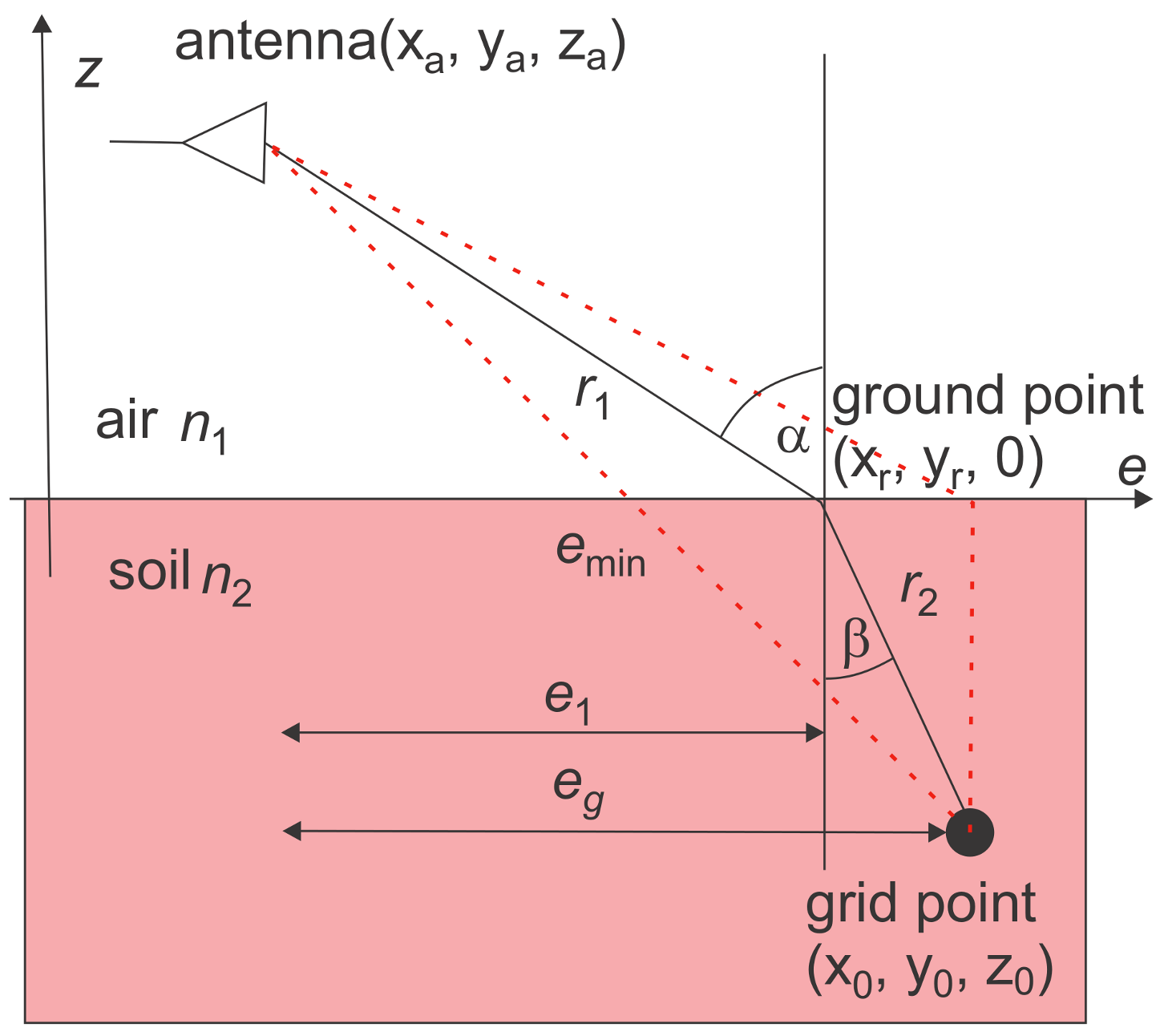
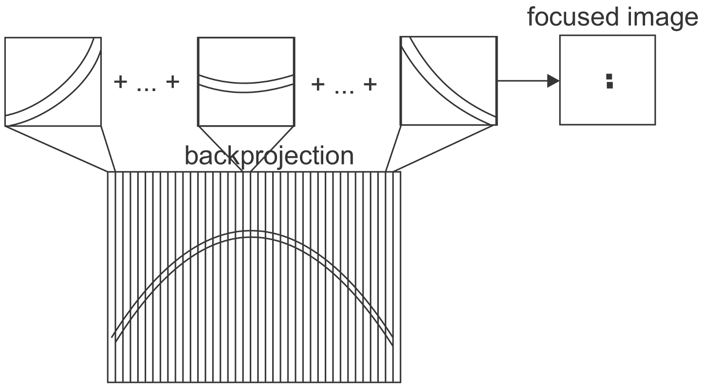
Back Projection Algorithm

The back-projection algorithm is depicted in Figure 2. It reconstructs an image by coherently summing radar returns for each pixel, considering the time delays between the radar and pixel location. The algorithm works by back-projecting the radar data onto the ground plane, compensating for range migration and phase changes caused by motion.

The matched filter and back-projection imaging algorithms [27] use a second-order Taylor series approximation of the differential range [28] in conjunction with the SAR signal model using polar format algorithm for spotlight SAR based on a linear approximation. The following subsection shortly summarizes the BP algorithm described in [27]. The radar sends out pulses that bounce off scatterers in the area at regular intervals. The radar then picks up some of the energy. The image is formed by receiving $N_p$ pulses at time instants $\left\{t_n\right|n=1,2,\dots ,N_p\}$. The receiver output at a specific time $t_n$ is a series of signals with different frequencies that experience propagation to the target and back which results in a delay in relation to the pulse transmission time. Each pulse consists of K signals with different frequencies, and the sequence $\left\{f_k\right|k=1,2,\dots ,K\}$ represents the corresponding frequency values. The received signal from scattering at target location r is given by

$$S(f_k,t_n)=A(f_k,t_n)exp\left(-j4\pi f_k(\Delta R^{\prime }\left(t_n\right)/v_1+\Delta R^{\prime \prime }\left(t_n\right)/v_2)\right),$$

(4)

where the amplitude, $A(f_k,t_n)$, represents the target’s radar cross section and the phase depends on the frequency of each sample and on the differential range, $\Delta R^{\prime }\left(t_n\right)$, given by

$$\Delta R^{\prime }\left(t_n\right)=d_{a_r}\left(t_n\right)-d_a\left(t_n\right).$$

(5)

$$\Delta R″\left(t_n\right)=d_{a_0}\left(t_n\right)-d_{a_r}\left(t_n\right).$$

(6)

The target location is given by $r\left(t\right)={[x_0\left(t\right);y_0\left(t\right);z_0\left(t\right)]}^T$, and it is assumed that the target is not moving. The radar cross section of the target varies with aspect angle and frequency. The distance is represented as the distance between the antenna phase center and the target. The antenna phase center of the SAR sensor has a three-dimensional spatial location, ${\mathbf{r}}_a\left(t\right)={[x_a\left(t\right);y_a\left(t\right);z_a\left(t\right)]}^T$, where t represents the slow time domain, also known as the synthetic aperture, and T represents the transpose operator. The distance between the antenna phase center and the origin is given by

$$d_a\left(t\right)=\sqrt{x_a{\left(t\right)}^2+y_a{\left(t\right)}^2+z_a{\left(t\right)}^2}.$$

(7)

The infliction point is given by $r_{a_r}\left(t\right)=[x_r\left(t\right);y_r\left(t\right);0){]}^T$, and the distance to it is

$$d_{a_r}\left(t\right)=\sqrt{{(x_a\left(t\right)-x_r\left(t\right))}^2+{(y_a\left(t\right)-y_r\left(t\right))}^2+z_a{\left(t\right)}^2}.$$

(8)

Distance from the infliction point to the target is given by

$$d_{a_0}\left(t\right)=\sqrt{{(x_r\left(t\right)-x_0\left(t\right))}^2+{(y_r\left(t\right)-y_0\left(t\right))}^2+z_0{\left(t\right)}^2}.$$

(9)

The frequency samples, $\left\{f_k\right\}$, are represented by the following values: $\Delta f$ represents the frequency step size, $f_1$ stands for the minimum value, $f_c$ for the central value, and $f_K$ for the maximum value. The frequency step size is inversely related to the maximum unambiguous range, $R_{max}={\displaystyle \frac{c}{2\Delta f}}$. As a result, the frequency step size is to correspond with maximum penetration depth. The used bandwidth is $B=(K-1)\Delta f$, and the range resolution is $\Delta R={\displaystyle \frac{c}{2B}}={\displaystyle \frac{c}{2(K-1)\Delta f}}$. The maximum alias-free cross-range extent of the image $W_x$, is determined by the azimuth angle from pulse to pulse. $W_x={\displaystyle \frac{{\lambda }_{\min }}{2\Delta \theta }}$, where ${\lambda }_{\min }$ is the smallest wavelength such that ${\lambda }_{\min }=c/f_K$, and the azimuth step size is denoted by $\Delta \theta$. During the synthetic aperture, the total azimuth angle, ${\theta }_a$, is traversed as follows: ${\theta }_a=(N_p-1)\Delta \theta$. Therefore, ${\Delta }_x$, the cross-range resolution, is evaluated as

$${\Delta }_x={\displaystyle \frac{{\lambda }_c}{2{\theta }_a}}={\displaystyle \frac{{\lambda }_c}{2(N_p-1)\Delta \theta }}.$$

(10)

where ${\lambda }_c$ is the central wavelength such that ${\lambda }_c=c/f_c$.

To prevent aliasing of the image or the frequency support, the total scene size should be smaller than the maximum scene and the pixel spacing should be finer than the range and azimuth resolution. One way to conceptualize the matched filter method to image generation is as a differential range computation for each pixel in each pulse. The response of the matched filter is represented by

$$I\left(r\right)=\sum _{n=1}^{N_p}\sum _{k=1}^{K}S(f_k;t_n)exp\left(j4\pi f_k(\Delta R^{\prime }\left(t_n\right)/v_1+\Delta R″\left(t_n\right)/v_2)\right)$$

(11)

The target response at a discrete range bin, m, can be calculated using the matched filter response (11). The range profile at range bin m given a received pulse at slow time $t_n$ is

$$s(m;t_n)=\sum _{k=1}^{K}S(f_k;t_n)exp\left(j4\pi f_k(\Delta R^{\prime }(m;t_n)/v_1+\Delta R″(m;t_n)/v_2)\right).$$

(12)

where $S(f_k;t_n)$ represents SAR phase history, collected by $N_p$ pulses over a range of K frequencies. By replacing $f_k=(k-1)\Delta f+f_1$ in (12) with the frequency values, the received pulse is given by

$$\begin{array}{cc}\hfill s(m;t_n)& =\sum _{k=1}^{K}S(f_k;t_n)\hfill \\ \hfill & exp[\mathsf{\Phi }(\Delta R(m;t_n))·(k-1)]exp\left(j4\pi f_1(\Delta R^{\prime }(m;t_n)/v_1+\Delta R″(m;t_n)/v_2)\right),\hfill \end{array}$$

(13)

where the phase function is

$$\mathsf{\Phi }(\Delta R(m;t_n))=(j4\pi \Delta f(\Delta R^{\prime }(m;t_n)/v_1+\Delta R″(m;t_n)/v_2)).$$

(14)

The backprojection algorithm using discrete implementation is given by

$$s(m;t_n)=K·\mathrm{ifft}\left(S(f_k;t_n)\right)·exp\left(j{\displaystyle \frac{2\pi f_1(m-1)}{K\Delta f}}\right).$$

(15)

where ifft(.) represents the fast inverse Fourier transform and K represents a scaling factor. Applying Equation (15) for each pulse and zero-padding the data so that the inverse fast Fourier transform (ifft) length becomes $N_{\mathrm{fft}}$ is the first stage in creating an image. Hence, $S(f_k;t_n)=0$ for all $k>K$, and

$$s(m;t_n)=N_{\mathrm{fft}}·\mathrm{fftshift}\left\{\mathrm{ifft}\left(S(f_k;t_n)\right)\right\}·exp\left(j{\displaystyle \frac{2\pi f_1(m-1)}{N_{\mathrm{fft}}\Delta f}}\right),$$

(16)

$\Delta R(m;t_n)$ is computed to provide the image response for a pixel at location r. $s(m;t_n)$ is then interpolated to compute $s_{\mathrm{int}}(r;t_n)$, which represents interpolated image response. The sum of these values for each pulse is the final image response, $I\left(r\right)$ given by

$$I\left(r\right)=\sum _{n=1}^{N_p}{s}_{\mathrm{int}}(r;t_n).$$

(17)

3. Methodology

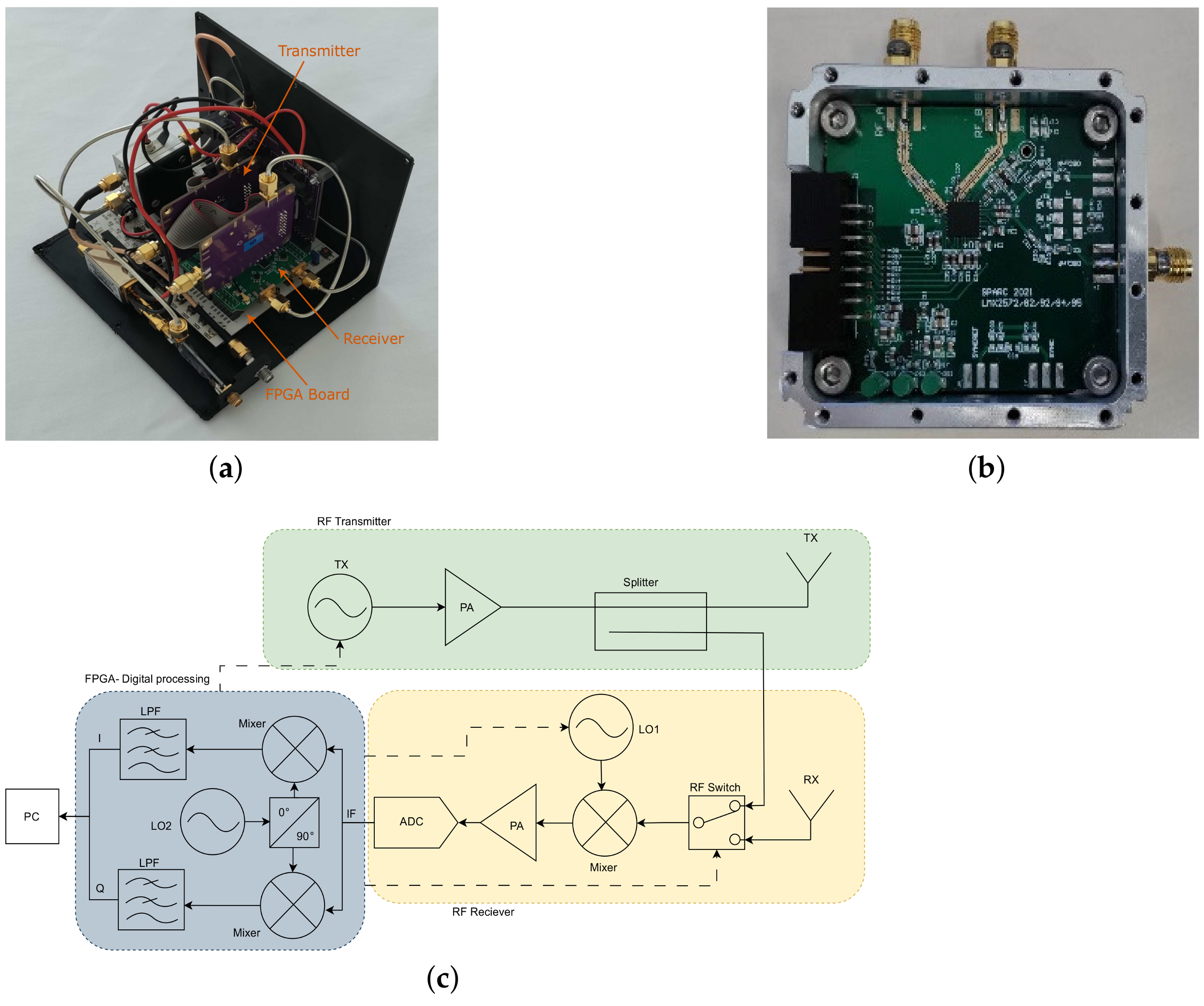
3.1. Radar System Design and Theory

The SFCW radar system used in this paper was developed in a preliminary study [29]. The developed SFCW radar features a modular design radar, as depicted in Figure 3. The modular architecture incorporates two frequency synthesizer boards, a receiver board with a signal mixer, a differential amplifier, and an analog-to-digital converter (ADC). Complementing these components are an RF switch, a low-noise amplifier, and a signal splitter. The presented radar operates within the 500 MHz to 2.5 GHz frequency range, with a 10 MHz frequency increment. It employs TI LMX2572 wideband RF synthesizers to generate TX (transmit) and LO (local oscillator) signals. At its core lies the Arty A7-35T: Artix-7 FPGA development board, facilitating efficient signal processing. The sampled data are transmitted to a personal computer via USB for subsequent processing. Figure 3a,b depict the modular radar design and the RF synthesizer, and Figure 3c shows the block diagram of the SFCW radar system.

The superheterodyne architecture of SFCW offers notable advantages. Converting the received signals to a fixed intermediate frequency enhances sensitivity and facilitates efficient filtering. This architecture allows for improved selectivity and ease of signal processing, contributing to enhanced target detection and discrimination. Overall, the superheterodyne architecture enhances the radar system performance, providing better signal quality, reduced interference, and increased accuracy in subsurface monitoring and other applications. To meet this requirement, a common clock source was used as a reference signal for both the FPGA and signal synthesizers. This setup ensures synchronized operation and accurate signal processing.

Given that each frequency step has a duration of 600 ms, a total of 200 steps were used within the designated bandwidth and,

$$R_{\max }={\displaystyle \frac{c}{2\Delta f}}$$

(18)

$$\Delta R={\displaystyle \frac{R_{\max }}{K}}={\displaystyle \frac{c}{2B}}$$

(19)

where $R_{max}$ is the unambiguous range, $\Delta R$ represents the radar resolution, c denotes the speed of light, $\Delta f$ signifies the change in frequency step, K denotes the number of pulses, and B stands for the occupied frequency band. In this context, K also represents the total number of frequency steps. The system is capable of theoretically achieving an unambiguous range of 15 m (18) and a resolution of 7.5 cm (19). The receiver employs a 14-bit ADC to capture the received signal, and it requires 125 ms to generate the transmitted signal and acquire received signals for all 200 frequency steps.

The radar’s average noise level of −60 dBm indicates a relatively low noise floor, which enhances its sensitivity to weak signals. This is illustrated in Figure 4, where both the measured noise floor and the averaged noise floor are displayed, using a moving average filter with a window size of 20 samples. A lower noise level is critical in radar systems, as it allows for the detection of faint echoes and improves the system’s ability to discern targets in challenging environments. The radar has a modular design that slightly raises the noise floor compared to a compact implementation [30]. Nevertheless, the −60 dBm noise level suggests a favorable signal-to-noise ratio, contributing to the radar’s overall performance and reliability. This is particularly advantageous in applications where accurate and reliable signal detection is paramount, ensuring the radar system’s effectiveness in various operational scenarios.

Choosing the right antenna for GPR systems depends on the measurement type. Antennas can either be ground-coupled, where they are in direct contact with the ground, or air-launched, where they are positioned at a distance from the ground. Ground-coupled systems involve a single propagation medium, allowing for a wider range of antenna types, particularly planar antennas. The signal in an air-launched system travels through both air and soil, leading to reflections at each transition and reducing the target amplitude. This setup complicates achieving effective coupling across a wide frequency band, especially at sub-GHz frequencies, due to the impedance mismatch between the radar feed line (typically 50 Ω) and air characteristic impedance (approximately 377 Ω). The antenna must handle this impedance transition smoothly to avoid internal reflections.

The S11, S22, and S12 parameters of the fabricated TEM horn antennas are shown in Figure 5a,b. These results indicate that both the reflection and transmission coefficients are satisfactory across the bandwidth of 500 MHz to 2.5 GHz.

TEM horn antennas are favored for their lightweight and compact design, utilizing thin copper film on a planar substrate. However, lower frequency bands required for GPR increase antenna size. The hybrid TEM horn antenna, proposed in [31], combines the advantages of both antenna types, converting the planar Vivaldi antenna into a 3D structure, which reduces the antenna size. The antenna depicted in Figure 6b, was fabricated from a 0.5 mm thick copper plate, measuring $95\mathrm{mm}\times 225\mathrm{mm}\times 180\mathrm{mm}$ and weighing $240\mathrm{g}$, suitable for medium payload UAVs.

The proposed radar poses a limitation to the UAV velocity. This performance is sufficient for low-velocity UAVs, but it is likely inadequate for high-velocity UAVs, which require faster data acquisition rates to accurately capture the rapidly changing positions and surroundings. Therefore, this system is suitable for low-velocity flight up to 1 m/s but not for high-velocity UAVs.

Additional limitation of proposed radar design is air-to-ground coupling, which will impact the penetration depth of the proposed system. In the air-coupled GPR system, there are four main factors affecting the penetration depth: transmitted power, dynamic range of the receiver, attenuation of the ground material, and center frequency of the transmitted signal. If we are only interested in how penetration depth will change with different GPR on different heights, it can be concluded that a center frequency and ground attenuation have a negligible impact on penetration depth change. Following the inverse-square law, the energy of the electro-magnetic field does not change over distance R, but the intensity $I\left(R\right)$ changes because the illuminated area gets larger with R. Therefore, if the height of the GPR above the ground doubles, the illuminated area gets four times larger and the intensity is reduced by $1/4$ or $1/R^2$. According to Beer–Lambert law, the penetration depth depends solely on the absorption coefficient, which does not change with the change in height. The penetration depth ${\delta }_p$ can be defined as:

$${\delta }_p={\displaystyle \frac{1}{\alpha }}$$

(20)

where $\alpha$ is the absorption coefficient. From the Beer–Lambert law, defined as:

$$I\left(z\right)=I_0·e^{-\alpha z}$$

(21)

where $I\left(z\right)$ is the intensity at depth z, and $I_0$ is the initial intensity, which concludes that the back reflected signal changes with the same coefficient at depth z as long as the absorption coefficient is constant. The measurable penetration depth ${\delta }_m$ is lower then the penetration depth ${\delta }_p$ and depends on the wave intensity at the ground surface and receiver noise-floor level. Since the transmitted power and receiver’s noise floor are not easily adjustable in the proposed GPR system, there is a point where the GPR height is not practical anymore and cannot be estimated without knowing the absorption coefficient of the ground. The measurement of the absorption coefficient of the ground material is not practical since the absorption coefficient will change with a different ground structure, and a constant $\alpha$ cannot be evaluated. The study of relation between the penetration depth and the height of the GPR above the ground surface is out of the scope of this paper and will not be further discussed.

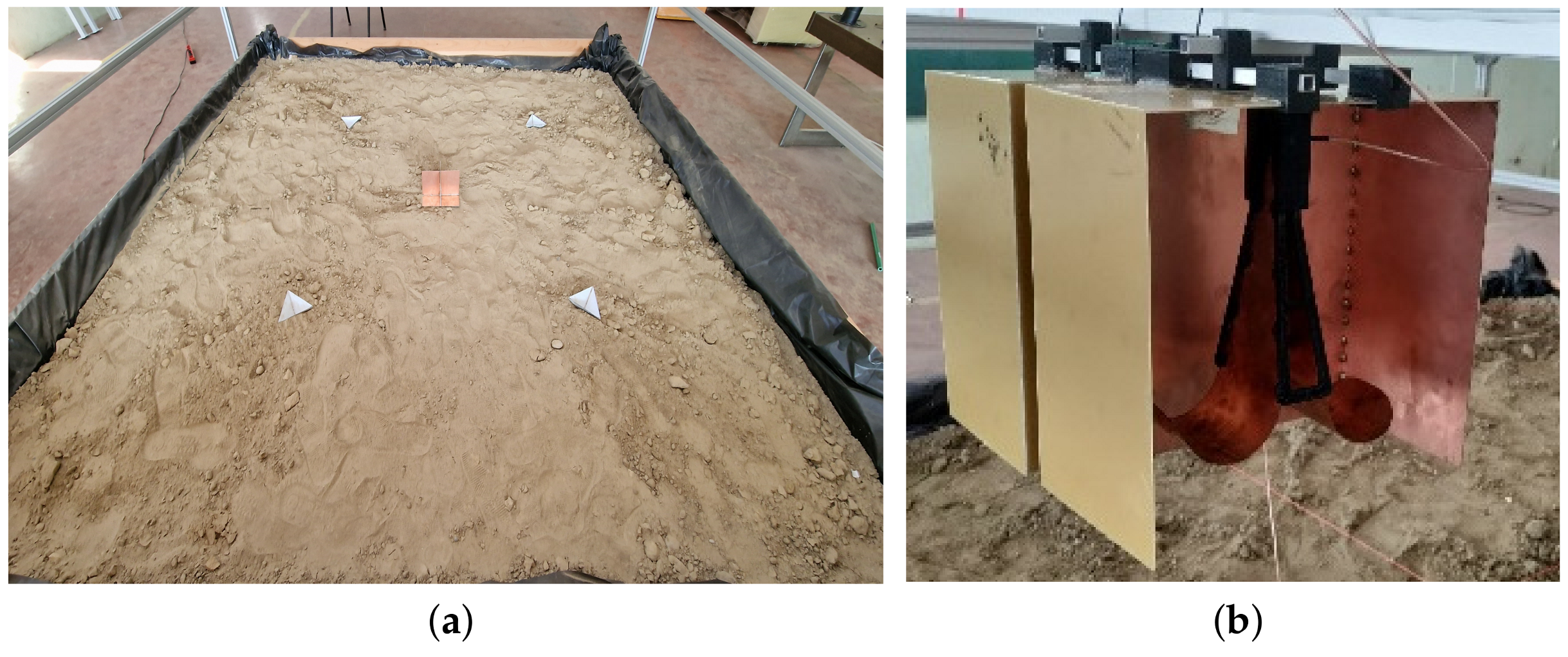
3.2. Experimental Setup

For experimental validation, the radar system was attached to a rail, moving orthogonal to its axis. Antennas used in experiments were positioned at a height of 0.55 m above the ground. TEM horn antennas were used as described in reference [29,31]. Figure 6a,b represent the experimental setup. This modular SFCW radar system, with its versatile design and comprehensive frequency range, holds promise for diverse subsurface monitoring applications.

Figure 7 illustrates various acquisition configurations based on the positioning and movement of the transmitter (TX) and receiver (RX) antennas, all operating in an air-coupled setting with antennas positioned 55 cm above the surface. The down-looking (DL) GPR configuration, as presented in Figure 7a, involves both the TX and RX antennas directed downward for subsurface investigation. Figure 7b shows a monostatic configuration, where TX/RX antennas adopt a side-looking orientation. The down-looking GPR configuration generates a GPR B-scan; meanwhile, the side-looking configuration can be configured as circular SAR or a radar platform, which is rotated around its Z axis.

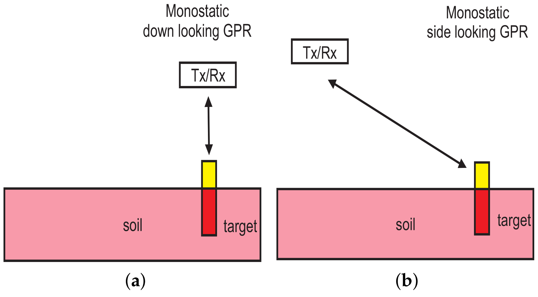
3.2.1. Down-Looking and Side-Looking GPR Configuration

The air-coupled down-looking GPR mode excels in providing greater depth penetration compared to side-looking mode [20,21]. By emitting radar signals directly downward and receiving reflections from subsurface features, it minimizes signal loss through the ground, enabling exploration of deeper geological layers, buried utilities, or archaeological structures. On the other hand, side-looking GPR mode offers advantages in terms of lateral resolution and imaging detail. By emitting and receiving signals perpendicular to the direction of travel, it provides high-resolution images of subsurface features laterally, enabling precise mapping of shallow subsurface structures such as pipes, cables, or foundations.

In side-looking GPR, the radar antenna is typically mounted on a cart or vehicle and pointed at a certain incidence angle. This setup allows the radar pulses to penetrate the ground and reflect off subsurface features to create a cross-sectional image of the subsurface. The system records the time taken for the radar pulses to travel to the subsurface and back, which is then processed to generate an image representing the depth and location of subsurface objects or layers. Side-looking GPR systems typically provide GPR images with a wider covered area [32] because the radar illuminates a wider area compared to a down-looking configuration. This enables detailed visualization of underground objects with more complex features. The side-looking configuration provides clear cross-sectional views of the subsurface, which aids in distinguishing between different types of targets. This clarity facilitates the recognition of targets based on their shape, size, and depth. Side-looking GPR systems are often capable of accurately determining the depth of subsurface targets. This depth of information helps in identifying the nature and significance of detected objects, improving target recognition.

Figure 8 illustrates the side looking, circular configuration of the radar, where the radar system is configured as monostatic radar, but the entire platform undergoes rotation around the yaw axis. In this unique setup, the surface is illuminated by an antenna beam, and the size of the illuminated area is contingent on the characteristics of the antenna employed. The resulting samples effectively represent the illuminated region, akin to the scenario encountered in side-looking GPR. In the case of side-looking GPR, the B-scans are intricately tied to the illumination angle, influencing the characteristics and information captured within each scan. The rotating antenna beam scans the subsurface, capturing variations in the illuminated region as it revolves. This side-looking configuration offers advantages in scenarios where a comprehensive overview of the subsurface is desired, providing a mechanism to cover a 360 degree swath. The size and characteristics of the illuminated area become critical considerations, influencing the resolution and coverage of the acquired data. Additionally, the rotation introduces variability in the incidence angle, affecting the interpretation of B-scans and contributing to the systems adaptability in different subsurface imaging scenarios. Understanding and optimizing the monostatic circular configuration are essential for harnessing its potential in subsurface monitoring applications. This configuration’s ability to provide a panoramic view of the subsurface, influenced by the rotating platform and antenna beam, positions it as a valuable tool in applications such as environmental monitoring, geological surveys, and infrastructure assessments, where a comprehensive understanding of subsurface structures is crucial.

The circular GPR SAR is a configuration where the radar antenna is mounted on a rotating platform, allowing it to emit radar pulses in multiple directions around the systems axis. As the antenna rotates, it collects radar data from different angles, which can then be combined and processed to create a two-dimensional or three-dimensional image of the subsurface. Circular GPR SAR collects radar data from multiple perspectives as the antenna rotates. This multi-angle approach enhances target recognition by providing a comprehensive view of the subsurface, reducing ambiguities in target identification. Circular GPR SAR can achieve higher resolution imaging compared to traditional side-looking GPR systems. By synthesizing data from different angles, it enhances the resolution of subsurface images, allowing for finer details to be discerned. The ability to gather data from various angles enables circular GPR SAR to better discriminate between different types of targets based on their scattering properties and geometric features. This enhances target recognition accuracy, particularly in complex environments. Circular GPR SAR can generate 2D images of the subsurface, providing additional information for target recognition. The ability to visualize targets in 3D enhances the understanding of their spatial distribution and relationship with surrounding features.

Figure 9 showcases a circular configuration where antennas are arranged in a monostatic configuration, yet the platform traces a circular trajectory. Typically employed in circular SAR configurations, this setup enables the acquisition of a 2D image of the designated area through the application of various focusing algorithms. The dimensions of the antennas footprint are determined by both the height of the platform and the beam-width of the antenna. This footprint, in turn, dictates the extent of the acquired area. In circular SAR configurations, the circular trajectory of the platform introduces a unique imaging perspective. As the platform traverses the circular path, the radar system captures information from different angles, contributing to the creation of a comprehensive and detailed image of the targeted region. The choice of focusing algorithms plays a crucial role in the synthesis of high-resolution images from the collected data. The size of the antennas footprint is a critical parameter influencing the imaging capabilities of the system. A balance between platform height and antenna beamwidth must be carefully considered to optimize the footprint size, ensuring that the acquired area meets the specific requirements of the application. This circular configuration finds relevance in applications requiring panoramic and detailed imaging, such as environmental monitoring, geological mapping, and terrain analysis. The distinctive circular trajectory enhances the systems versatility, making it adept at capturing intricate details across the entire designated area.

3.2.2. Acquisition Scenarios

Two corner reflectors were placed on the top of the indoor polygon, as shown in Figure 10. Corners were separated by 0.5 m, and in the second scenario, they were buried at a depth of 0.2 m. Corners consist of a tetrahedron without base with a size length of 10 cm. The scene was the same for all three scenarios. The antennas were positioned at a constant height of 55 cm.

The scenarios for the three experiments are shown in Figure 11 and are depicted as top-down views within a 3 × 3 m polygon. Corner locations are marked with an ‘x’, and the starting position of the antennas is indicated by a circled ‘1’. The trajectory of the platform in the down-looking configuration spanned 150 cm (Figure 11a, marked with a red dashed line). The platform was moving at a speed of 2 cm/s, leading to a total data collection time of 75 s. The starting position is marked as ‘1’, and the end position as ‘2’. In the side-looking configuration where the platform rotated around the z-axis (Figure 11b), the data collection time was 86 s and the angular rotation speed was around 2.1 °/s. For the side-looking circular measurements (Figure 11c), the trajectory was 345 cm long, and had the same movement speed of 2 cm/s; the data collection time was 172 s. As the circular trajectory was performed, the start and end points were the same. The antennas were directed toward the center, with the initial orientation marked by an arrow pointing outward from the circled ‘1’. The circular trajectory is marked in a dashed red line.

4. Experimental Results

All experiments were conducted within a custom-designed indoor polygon measuring $3\times 3\times 0.5$ m, as illustrated in Figure 6a. To facilitate movement in two degrees of freedom for the radar platforms, a two-dimensional rail system was constructed above the polygon.

The soil volumetric moisture was 5% on the top of the polygon and 14% at the bottom of the polygon at a temperature of 21 °C. The soil moisture was measured using SWM-5000 soil moisture meter [33]. The soil is depicted in Figure 12, and has a very small granular structure of 0.1 mm. The test material was a mixture of sand (90%) and clay (10%). Pure sand typically has a dielectric constant ranging from 2 to 3, while the dielectric constant of clay is much higher, typically ranging from 5 to 15. Given that there is a high proportion of sand and an absence of moisture, a lower dielectric constant is expected, possibly in the range of 2 to 5. A low moisture level indicates lower loss compared to wet soil, as the water in the soil absorbs more energy from waves passing through, leading to greater attenuation.

Initially, tests were conducted using both HH and VV polarization. The corner reflector was buried 0.4, 0.6, and 0.8 m below the surface. For these measurements, a portion of the polygon was raised, and additional soil was added to allow for deeper target burial, as the original polygon was only 0.5 m deep. Figure 13a–f show B-scans of the targets with removed background. Figure 13a,b show that targets can be clearly identifies in both polarization’s. Targets are hardly visible at the depth of 0.6 m, as depicted in Figure 13c,d. Targets can not be detected at a depth of 0.8 m. Based on these experiments, VV polarization gives smaller intensities, but the signatures are more visible.

The acquired signals in the frequency domain underwent transformation through the inverse Fourier transform, with an additional 300 samples to improve resolution. This processing step is essential for converting frequency–domain data into a more interpretable time–domain representation. The experiments were designed to encompass three distinct scenarios, as depicted in Figure 7, Figure 8 and Figure 9. For each scenario, corner reflectors were strategically placed as targets. In the first set of scenarios, these corner reflectors were positioned above the surface, facilitating adjustments to the platform.

In the second scenario, the corner reflectors were buried at a depth of 20 cm below the surface. Although Figure 14 does not show a good signal-to-clutter ratio for a target at this depth, it is crucial to consider the conditions under which this measurement was made. Figure 14 illustrates a small buried corner reflector with side lengths of 10 cm. Notably, the reflection from the bottom of the soil box is visible at the 50 cm mark, demonstrating some signal detection capabilities under these specific test conditions. Under favorable conditions with a high radar cross-section target such as an anti-tank landmine, objects can be detected at depths of up to 0.6 m. Additionally, in practical applications, especially in landmine detection, the interest predominantly lies in identifying objects near the subsurface, where the radar’s ability to detect larger metallic objects remains relevant and effective.

The utilization of corner reflectors as targets adds a practical dimension to the experiments, simulating real-world scenarios where radar systems are deployed to detect and characterize objects or anomalies within a subsurface environment. The deliberate variation in the placement of the corner reflectors, both above and below the surface, introduces complexity to the experiments, enabling a thorough evaluation of the SFCW radar platform performance in different subsurface conditions. The custom-designed indoor polygon and rail system provide a controlled yet versatile environment for systematically exploring the capabilities and limitations of the radar system under various experimental scenarios.

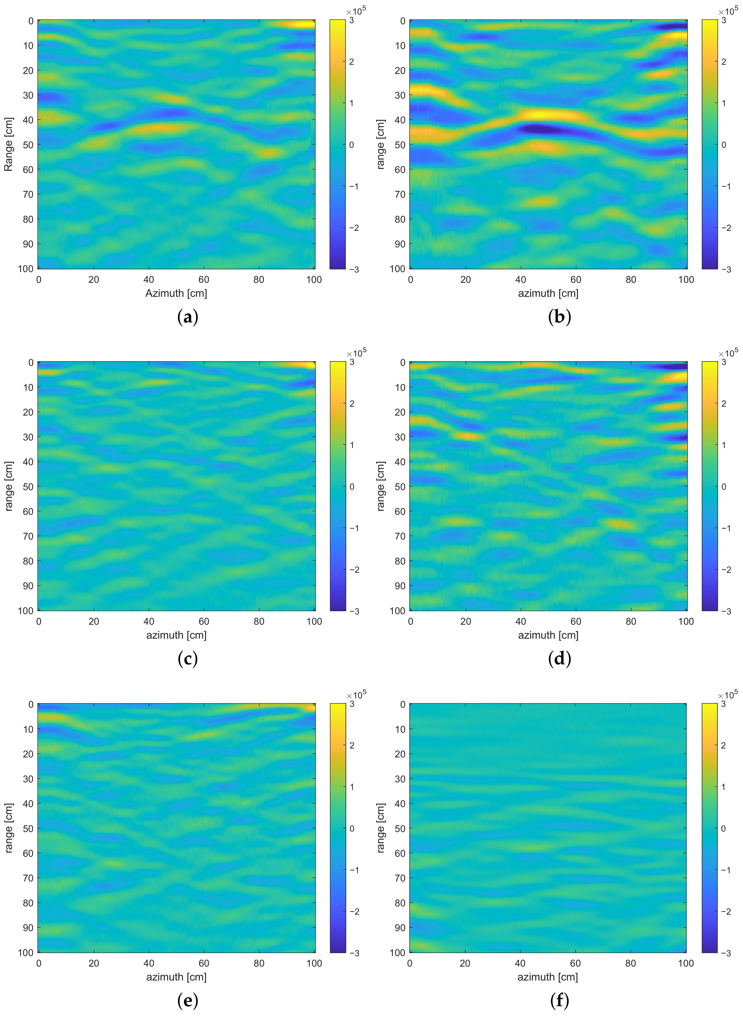
4.1. Monostatic Down-Looking Configuration

In Figure 14, B-scans obtained using the monostatic down-looking configuration are depicted. The effective coverage area extends to 2.7 m in the azimuth direction and approximately 0.1 m in the range direction. Corners were separated by 0.5 m. The hyperbolic reflections from the corners provide a clear indication of the radar system’s ability to capture and interpret subsurface features in a down-looking configuration. The effective coverage dimensions underscore the system capability to scan a specific area with precision, contributing to a detailed and accurate representation of the subsurface environment. Figure 14a–d show that the target signature is the most visible in the VV polarization, although the amplitude is approximately two-times smaller compared with the case of VV polarization.

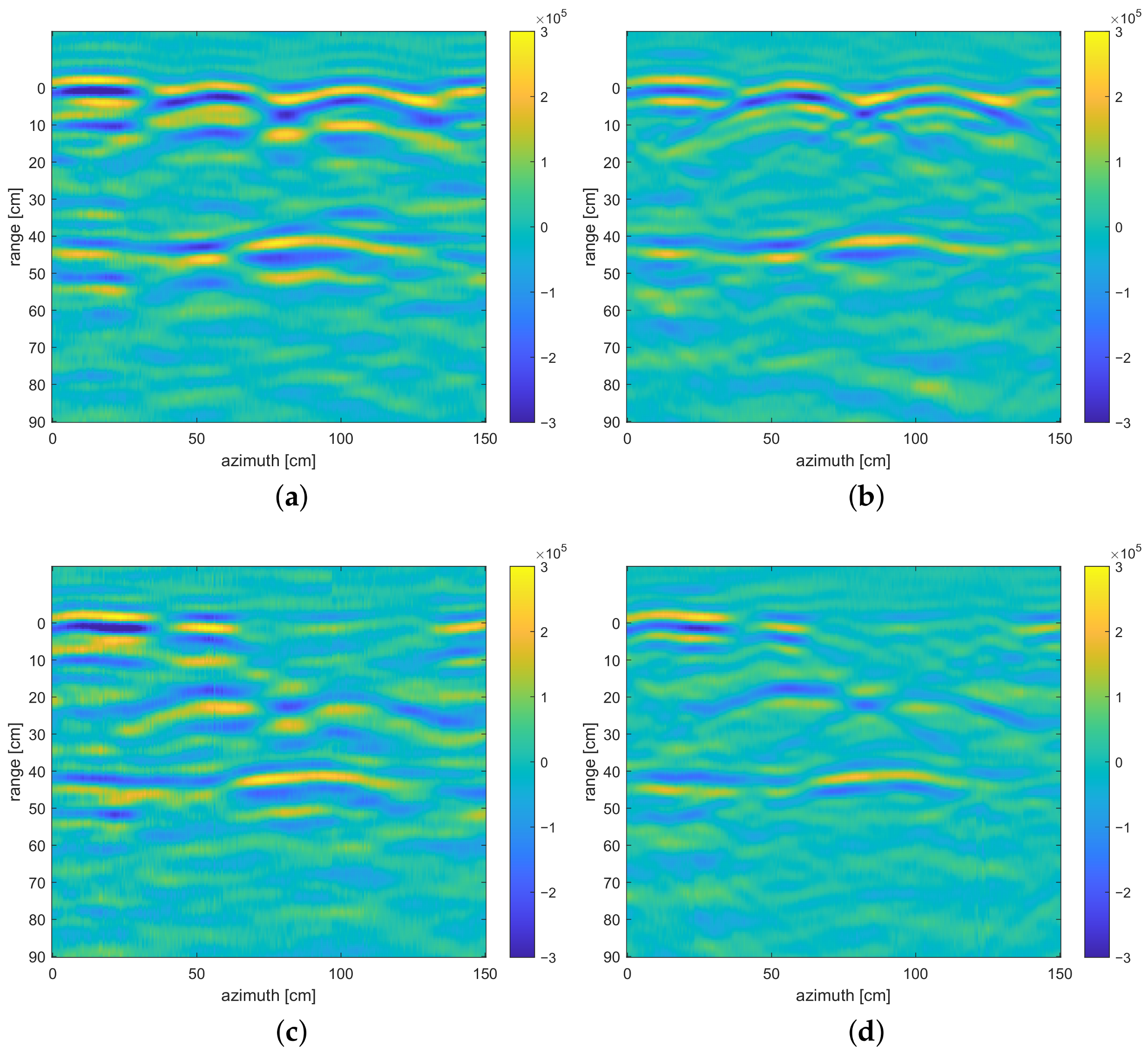
4.2. Monostatic Side-Looking Configuration

Figure 15 shows a monostatic side-looking configuration presented in Figure 8, where the platform rotates arround its z-axis at the edge of the polygon with a 45-degree incidence angle. Targets can be effectively detected within a range of 0.9 m. This configuration offers a unique perspective as the radar system captures echoes and reflections from subsurface targets at a specific angle of incidence. The 45-degree incidence angle, combined with the platforms movement around its z-axis at the polygons edge, contributes to the systems ability to detect and characterize targets within the specified range. Figure 15a,b shows the HH and VV B-scans with the background removed for the targets placed on the surface. Figure 15c,d depict focused images using BP algorithm. Targets are clearly focused. Target profiles were analyzed using full width at a half maximum (FWHM) [34] and the FWHM measurements are compared in

Table 1. Full Width at half maximum (FWHM) measurements for focused images.

Figure	Polarization	FWHM Horizontal	FWHM Vertical	Ratio
Figure 15c	HH	26	57	0.44
Figure 15d	VV	26	70	0.36
Figure 16c	HH	64	76	0.84
Figure 16d	VV	25	64	0.4
Figure 17c	HH	62	62	1
Figure 17d	VV	62	50	1.24
Figure 18c	HH	62	111	0.56
Figure 18d	VV	62	72	0.98

. From Table 1 and Figure 15c,d, it can be concluded that both measurements provide the same quality of the focused targets.

The same targets were buried 20 cm below the surface. The B-scans, shown in Figure 16a,b, show the acquired data in HH and VV polarization, where the hyperbolas can be observed within the acquired data. Figure 16c,d represent focused images obtained after applying the BP algorithm to B-scans with the background removed. By using the BP algorithm, the data can be focused and the target can be better presented visually. The HH polarization in this case gives unusable results. The FWHM measurements showed that the VV polarization gives the best focused image, when FWHM is considered.

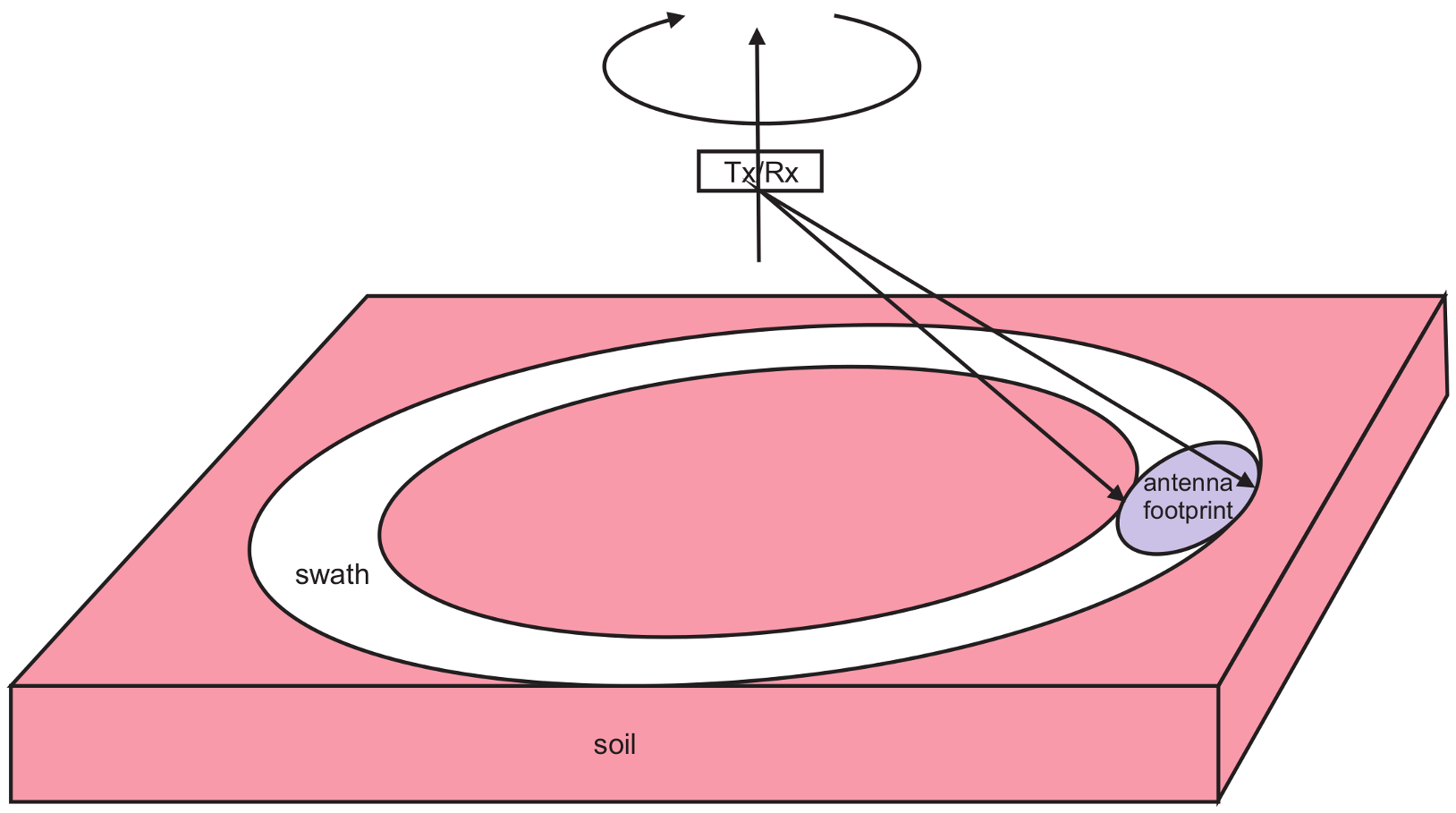
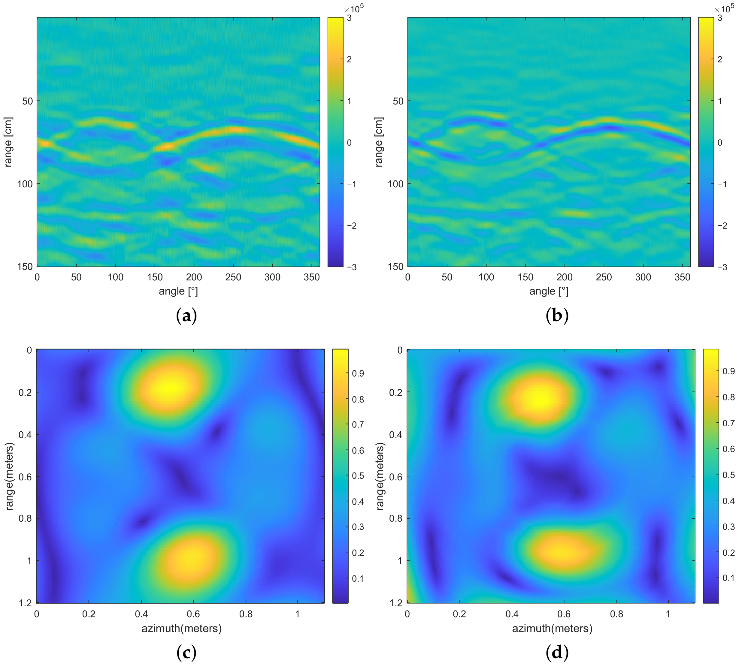
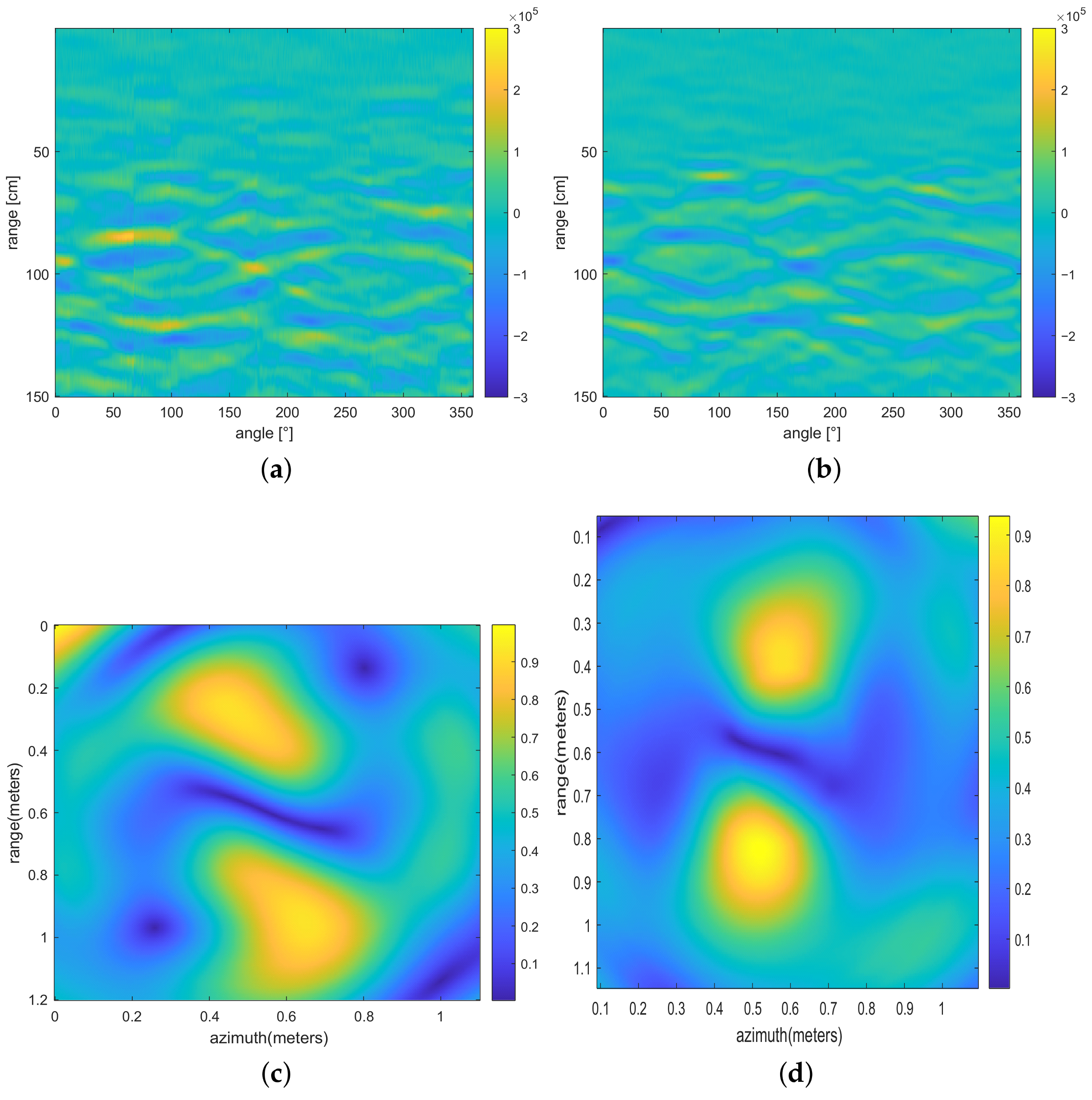
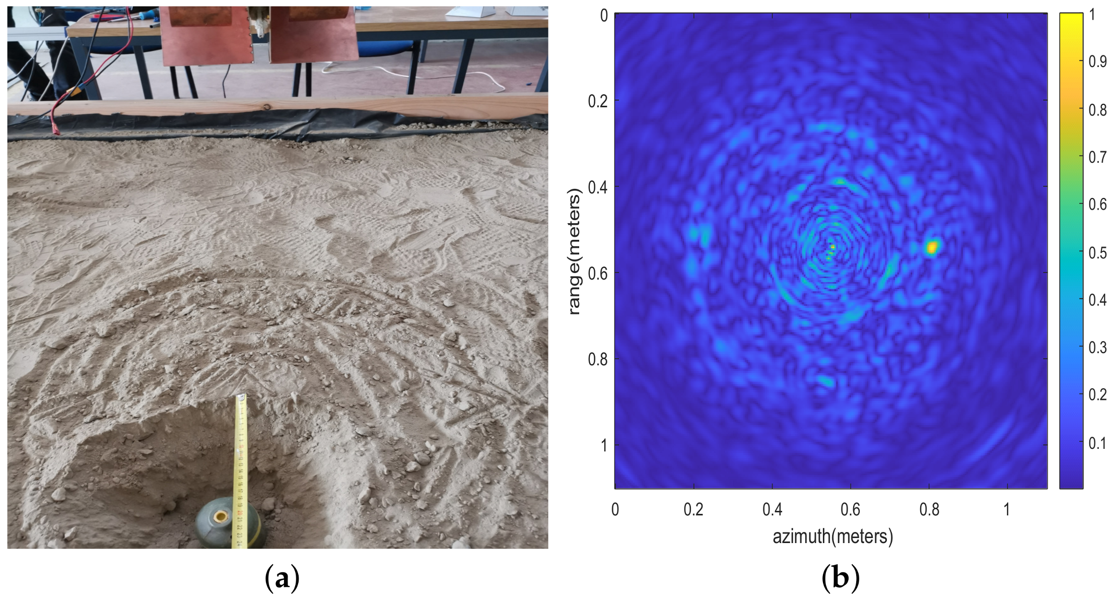
4.3. Circular GPR Configuration

Figure 17 illustrates the results achieved by moving the platform along a circular trajectory. Targets become discernible through the observation of hyperbolic patterns within the B-scans. The distinctive hyperbolas within the scan data indicate the presence and characteristics of subsurface targets, providing valuable insights into the radar system’s performance during circular acquisition. This representation aids in the identification and analysis of features within the scanned area, contributing to a comprehensive understanding of the subsurface environment under the circular acquisition configuration. Figure 17a,b depict the B-Scan obtained using GPR and targets on the surface using HH and VV polarization. The processed B-scan with background removal and the focused image using the BP algorithm for HH and VV polarization are shown in Figure 17c and Figure 17d, respectively. Targets are clearly focused in Figure 17c,d.

The same targets were buried 20 cm below the surface. The same processing chain was applied to the acquired GPR data. Figure 18a,b show the B-scan with removed background, and the focused images using the BP algorithm are shown in Figure 18c,d. The HH polarization does not provide very clear and focused targets, as can be noticed in Figure 18c. The results in Table 1 also indicate that the focused target is smeared.

The last experiment shows the scenario where the metal anti-personnel (AP) land mine, with a cylindrical shape with dimensions of 8 × 13 cm (diameter × height), placed in an upright position, was buried 20 cm below the surface, as shown in Figure 19a; the processed BP image is shown in Figure 19b, where the target is clearly seen. The results are presented only for VV polarization.

4.4. Discussion

This manuscript compared the down-looking and side-looking configurations using GPR acquisition. The main drawback of the down-looking configuration is that the area perpendicular to the antenna is illuminated. This makes the GPR system very limited when a larger area has to be scanned. This paper investigates the possibilities of using side-looking configurations that illuminate a wider area but require the focusing algorithm to interpret the data. The conclusion is that side-looking illumination of the area using the GPR enables us to acquire data more efficiently. All experiments showed that the circular SAR using the BP focusing algorithm visually better presents targets by focusing the hyperbolas from GPR B-scans into clearly defined image pixels that represent targets. Considering that the used antennas have 40 degrees of beam width, that the antennas were positioned at a 45 degree incidence angle, the platform was 0.55 m above the surface, and the radar illuminated an area of approximately 1.2 square meters. By applying circular SAR, we can cover the area with a diameter of 2.4 m or an area of 4.5 square meters. The radar platform travels a path of 3.7 m. The down-looking radar can cover the same area in a rectangular scan by illuminating an area 0.7 m wide that requires 3 scans separated by 0.7 m and by a traveling path of 2.4 m, which results in a total path of 7.2 m. The circular SAR provides acquisitions approximately two times faster (assuming that six turns take some additional time) than the down-looking platform, and, also, provides focused data. Processing the data took about 3 s on a PC-based machine with an I9 processor of 14th generation. An acquisition using the side-looking mode requires that the platform can be rotated around the Z axis. It covers 3.39 square meters if the platform is rotated 180 degrees or 6.7 square meters if the platform is rotated 360 degrees. This kind of acquisition is the most effective regarding the consumed time and the illuminated area.

All three presented scenarios were performed using HH and VV polarization, and each polarization was processed separately. Experimental results show that the VV polarization provides richer signatures for buried targets and provides more reliable results. The target response in the side-looking configuration is not ideal because the background removal algorithm was not able to clearly remove the background, but some clutter remained around the hyperbolic response, which was later focused on using the BP algorithm and some additional clutter appeared within the focused image using the side-looking configuration. The B-SCAN of the down-looking configuration is also very similar and would produce very similar results.

Several factors limit the performance of the proposed system, which must be carefully considered during the acquisition process. One key factor is penetration depth, which constrains radar performance and is heavily influenced by soil type. Our results show that the radar can detect targets up to 0.6 m below the surface. Another critical parameter is the height of the radar; the maximum theoretical ambiguous range of the SFCW radar is 15 m, which would limit the height of moving platform to 10 m at the antenna incidence angle of 45°.

Antenna beam width and angle are also important. We used a TEM antenna designed for air-coupled systems on a UAV. Once the system is set up, a B-scan is acquired, and background noise is removed. However, background removal must be performed carefully to avoid introducing clutter or false signatures. In side-looking scenarios, clutter appeared in the focused image due to the background removal algorithm.

The tests were conducted in an indoor environment, which may have caused some signal bouncing from nearby objects. Additionally, the 2D moving platform, made from aluminum, contributed to additional reflections. Despite these challenges, the best focusing results were obtained using circular SAR, with targets well-focused in all acquisitions.

This study’s use of GPR technology, as discussed in this paper, could be used in archaeological surveys to detect buried structures, artifacts, or other remains without excavation, especially when large areas need to be covered. There are also many practical applications in military applications, detecting buried objects makes it relevant for landmine detection, unexploded ordnance identification, or tunnel detection. The side-looking and circular acquisition methods could increase area coverage, improving efficiency in dangerous environments.

5. Conclusions

We laid out a comprehensive evaluation of various GPR acquisition scenarios, providing the basis for the potential application of these scenarios using UAVs to carry the radar system. The investigation included a down-looking monostatic and two circular acquisition modes, the first one involving platform rotation around the Z-axis, and, the second one, moving the platform along a circular trajectory. The experiments performed using a controlled polygon of dimensions $3\times 3\times 0.5$ m showed valuable insights. The presented radar design is capable of detecting targets buried up to 0.6 m below the surface.

The results demonstrated that the down-looking, side-looking, and circular-based acquisitions exhibited the ability to scan areas of up to 1.5 m in range or azimuth direction, particularly when the platform was positioned at a height of 0.55 m above the surface. These findings underscore the adaptability and effectiveness of these acquisition configurations in capturing subsurface information within defined coverage areas.

Regarding the novelty of this study, two contributions stand out. First, this paper offers a comparative analysis of three distinct GPR acquisition methods: down-looking, side-looking, and circular acquisition using an air-coupled SFCW radar system. Unlike most previous studies that focus on one method, this comprehensive comparison provides a detailed evaluation of each method’s coverage, penetration, and resolution, offering insights into their relative strengths and weaknesses. Second, the paper explores the underutilized circular SAR acquisition configuration with side-looking GPR. This approach provides complete area coverage, making it highly effective for detecting shallow buried objects and enabling faster and more accurate scanning of larger areas compared to traditional down-looking configurations.

Future research will concentrate on the development of sophisticated focusing algorithms tailored for monostatic circular acquisitions. The implementation of these algorithms aims to enhance the quality and interpretability of the acquired data, contributing to more accurate subsurface imaging. Additionally, there will be a focus on advancing automated target detection and recognition methodologies. The goal is to streamline the identification process, enabling efficient and precise detection and recognition of subsurface targets using the acquired data. Integrating GPRs with UAVs holds promise for revolutionizing subsurface sensing capabilities in diverse fields. The ability to deploy GPR systems on UAV platforms provides mobility and access to challenging terrains, facilitating rapid and cost-effective surveys. As technology continues to advance, the integration of sophisticated focusing algorithms, automated target detection, and recognition mechanisms will play a pivotal role in maximizing the efficiency and reliability of UAV-based GPR systems.

References

1. Catapano, I.; Gennarelli, G.; Ludeno, G.; Noviello, C.; Esposito, G.; Soldovieri, F. Contactless Ground Penetrating Radar Imaging: State of the art, challenges, and microwave tomography-based data processing. IEEE Geosci. Remote Sens. Mag. 2022, 10, 251–273. [Google Scholar] [CrossRef]
2. Dai, Q.; Lee, Y.H.; Sun, H.H.; Ow, G.; Yusof, M.L.M.; Yucel, A.C. 3DInvNet: A Deep Learning-Based 3D Ground-Penetrating Radar Data Inversion. IEEE Trans. Geosci. Remote Sens. 2023, 61, 1–16. [Google Scholar] [CrossRef]
3. Rodríguez-Santalla, I.; Gomez-Ortiz, D.; Martín-Crespo, T.; Sánchez-García, M.J.; Montoya-Montes, I.; Martín-Velázquez, S.; Barrio, F.; Serra, J.; Ramírez-Cuesta, J.M.; Gracia, F.J. Study and Evolution of the Dune Field of La Banya Spit in Ebro Delta (Spain) Using LiDAR Data and GPR. Remote Sens. 2021, 13, 802. [Google Scholar] [CrossRef]
4. Qiu, Z.; Zeng, J.; Tang, W.; Yang, H.; Lu, J.; Zhao, Z. Research on Real-Time Automatic Picking of Ground-Penetrating Radar Image Features by Using Machine Learning. Horticulturae 2022, 8, 1116. [Google Scholar] [CrossRef]
5. Fu, L.; Liu, S.; Liu, L.; Lei, L. Development of an Airborne Ground Penetrating Radar System: Antenna Design, Laboratory Experiment, and Numerical Simulation. IEEE J. Sel. Top. Appl. Earth Obs. Remote Sens. 2014, 7, 761–766. [Google Scholar] [CrossRef]
6. Ŝipoŝ, D.; Planinŝiĉ, P.; Gleich, D. Simulation and Implementation of Air-Coupled SFCW Radar on VNA. In Proceedings of the 2018 25th International Conference on Systems, Signals and Image Processing (IWSSIP), Maribor, Slovenia, 20–22 June 2018; pp. 1–4. [Google Scholar] [CrossRef]
7. García Fernández, M.; Álvarez Narciandi, G.; Arboleya, A.; Vázquez Antuña, C.; Andrés, F.L.H.; Álvarez López, Y. Development of an Airborne-Based GPR System for Landmine and IED Detection: Antenna Analysis and Intercomparison. IEEE Access 2021, 9, 127382–127396. [Google Scholar] [CrossRef]
8. Peters, L.; Daniels, J.; Young, J. Ground penetrating radar as a subsurface environmental sensing tool. Proc. IEEE 1994, 82, 1802–1822. [Google Scholar] [CrossRef]
9. Soumekh, M. Synthetic Aperture Radar Signal Processing; Wiley: New York, NY, USA, 1999. [Google Scholar]
10. Jol, H.M. Ground Penetrating Radar: Theory and Applications; Elsevier: Amsterdam, The Netherlands, 2009. [Google Scholar]
11. Wu, K.; Rodriguez, G.A.; Zajc, M.; Jacquemin, E.; Clément, M.; De Coster, A.; Lambot, S. A new drone-borne GPR for soil moisture mapping. Remote Sens. Environ. 2019, 235, 111456. [Google Scholar] [CrossRef]
12. Zhang, X.; Yang, C.; Xiao, Z.; Lu, B.; Zhang, J.; Li, J.; Liu, C. A novel target state detection method for accurate cardiopulmonary signal extraction based on FMCW radar signals. Front. Physiol. 2023, 14, 1206471. [Google Scholar] [CrossRef]
13. Pereira, M.; Burns, D.; Orfeo, D.; Zhang, Y.; Jiao, L.; Huston, D.; Xia, T. 3-D Multistatic Ground Penetrating Radar Imaging for Augmented Reality Visualization. IEEE Trans. Geosci. Remote Sens. 2020, 58, 5666–5675. [Google Scholar] [CrossRef]
14. Tosti, F.; Gennarelli, G.; Lantini, L.; Catapano, I.; Soldovieri, F.; Giannakis, I.; Alani, A.M. The Use of GPR and Microwave Tomography for the Assessment of the Internal Structure of Hollow Trees. IEEE Trans. Geosci. Remote Sens. 2022, 60, 1–14. [Google Scholar] [CrossRef]
15. Lei, Y.; Jiang, B.; Su, G.; Zou, Y.; Qi, F.; Li, B.; Jia, F.; Tian, T.; Qu, Q. Application of Air-Coupled Ground Penetrating Radar Based on F-K Filtering and BP Migration in High-Speed Railway Tunnel Detection. Sensors 2023, 23, 4343. [Google Scholar] [CrossRef] [PubMed]
16. Edemsky, D.; Popov, A.; Prokopovich, I.; Garbatsevich, V. Airborne Ground Penetrating Radar, Field Test. Remote Sens. 2021, 13, 667. [Google Scholar] [CrossRef]
17. Liu, P.; Ding, Z.; Zhang, W.; Ren, Z.; Yang, X. Using Ground-Penetrating Radar and Deep Learning to Rapidly Detect Voids and Rebar Defects in Linings. Sustainability 2023, 15, 11855. [Google Scholar] [CrossRef]
18. Vergnano, A.; Franco, D.; Godio, A. Drone-Borne Ground-Penetrating Radar for Snow Cover Mapping. Remote Sens. 2022, 14, 1763. [Google Scholar] [CrossRef]
19. González-Díaz, M.; García-Fernández, M.; Álvarez López, Y.; Las-Heras, F. Improvement of GPR SAR-Based Techniques for Accurate Detection and Imaging of Buried Objects. IEEE Trans. Instrum. Meas. 2020, 69, 3126–3138. [Google Scholar] [CrossRef]
20. García-Fernández, M.; Álvarez Narciandi, G.; Álvarez López, Y.; Las-Heras Andrés, F. Analysis and Validation of a Hybrid Forward-Looking Down-Looking Ground Penetrating Radar Architecture. Remote Sens. 2021, 13, 1206. [Google Scholar] [CrossRef]
21. Noviello, C.; Gennarelli, G.; Esposito, G.; Ludeno, G.; Fasano, G.; Capozzoli, L.; Soldovieri, F.; Catapano, I. An Overview on Down-Looking UAV-Based GPR Systems. Remote Sens. 2022, 14, 3245. [Google Scholar] [CrossRef]
22. Mohammadpoor, M.; Abdullah, R.S.A.R.; Ismail, A.; Abas, A.F. A circular synthetic aperture radar for on-the-ground object detection. Prog. Electromagn. Res. 2012, 122, 269–292. [Google Scholar] [CrossRef]
23. Mohammadpoor, M.; Abdullah, R.R.; Ismail, A.; Abas, A. A ground based circular synthetic aperture radar. In Proceedings of the 2013 14th International Radar Symposium (IRS), Dresden, Germany, 19–21 June 2013; Volume 1, pp. 521–526. [Google Scholar]
24. Grathwohl, A.; Arendt, B.; Grebner, T.; Waldschmidt, C. Detection of Objects Below Uneven Surfaces with a UAV-Based GPSAR. IEEE Trans. Geosci. Remote Sens. 2023, 61, 1–13. [Google Scholar] [CrossRef]
25. García Fernández, M.; Álvarez López, Y.; Arboleya Arboleya, A.; González Valdés, B.; Rodríguez Vaqueiro, Y.; Las-Heras Andrés, F.; Pino García, A. Synthetic Aperture Radar Imaging System for Landmine Detection Using a Ground Penetrating Radar on Board a Unmanned Aerial Vehicle. IEEE Access 2018, 6, 45100–45112. [Google Scholar] [CrossRef]
26. Saleh, B.; Teich, M. Fundamentals of Photonics; John Wiley and Sons: Hoboken, NJ, USA, 2007. [Google Scholar]
27. Gorham, L.A.; Moore, L.J. SAR image formation toolbox for MATLAB. In Proceedings of the Algorithms for Synthetic Aperture Radar Imagery XVII, Orlando, FL, USA, 5–9 April 2010; Volume 7699, p. 769906. [Google Scholar] [CrossRef]
28. Rigling, B.; Moses, R. Taylor expansion of the differential range for monostatic SAR. IEEE Trans. Aerosp. Electron. Syst. 2005, 41, 60–64. [Google Scholar] [CrossRef]
29. Šipoš, D.; Gleich, D. A Lightweight and Low-Power UAV-Borne Ground Penetrating Radar Design for Landmine Detection. Sensors 2020, 20, 2234. [Google Scholar]
30. Smogavec, P.; Pongrac, B.; Gleich, D. Evaluation of Compact and Modular SFCW GPR Systems for Detecting Buried Objects. In Proceedings of the 2023 30th International Conference on Systems, Signals and Image Processing (IWSSIP), Ohrid, North Macedonia, 27–29 June 2023; pp. 1–5. [Google Scholar] [CrossRef]
31. Ahmed, A.; Zhang, Y.; Burns, D.; Huston, D.; Xia, T. Design of UWB Antenna for Air-Coupled Impulse Ground-Penetrating Radar. IEEE Geosci. Remote Sens. Lett. 2016, 13, 92–96. [Google Scholar] [CrossRef]
32. Wu, M.; Ferro-Famil, L.; Boutet, F.; Wang, Y. Comparison of Imaging Radar Configurations for Roadway Inspection and Characterization. Sensors 2023, 23, 8522. [Google Scholar] [CrossRef]
33. GmBH, S.S. SWM 5000 Soil Moisture Meter. Available online: https://www.stepsystems.de/en/products/moisture-measurement/soil-moisture/swm-5000 (accessed on 24 September 2024).
34. Weik, M.H. Full-width at half-maximum. In Computer Science and Communications Dictionary; Springer: Boston, MA, USA, 2001; p. 661. [Google Scholar] [CrossRef]
Figure 1. Geometry illustrating Snell’s law.
Remotesensing 16 03931 g001
Figure 2. Backprojection algorithm.
Remotesensing 16 03931 g002
Figure 3. (a) Modular SFCW radar system, (b) signal synthesis board, (c) block diagram of modular SFCW radar.
Remotesensing 16 03931 g003
Figure 4. Noise level for modular SFCW radar.
Remotesensing 16 03931 g004
Figure 5. S11, S22, (a) and S12 (b) parameters of TEM horn antennas.
Remotesensing 16 03931 g005
Figure 6. (a) Soil-box used as a test polygon of 3 × 3 × 0.5 m. (b) TEM horn antennas [31].
Remotesensing 16 03931 g006
Figure 7. Different configuration of the transmitter and receiver. (a) Monostatic GPR, (b) monostatic side-looking GPR.
Remotesensing 16 03931 g007
Figure 8. Side-looking configuration. The platform is at the center position, and it is rotating around the Z axis.
Remotesensing 16 03931 g008
Figure 9. Circular SAR geometry. Platform is moving along circular trajectory.
Remotesensing 16 03931 g009
Figure 10. (a) Position of corners placed on the top of the surface. Corners were separated by 0.5 m. (b) Geometry of the data acquisition for side-looking SAR.
Remotesensing 16 03931 g010
Figure 11. The scenarios are depicted as top-down views within a 3 × 3 m polygon. (a) Trajectory of the down-looking scenario. (b) Scenario of side-looking experiment while rotating around z-axis. (c) Scenario of side-looking experiment with circular trajectory.
Remotesensing 16 03931 g011
Figure 12. Photograph of soil structure.
Remotesensing 16 03931 g012
Figure 13. B-Scans with removed background of targets buried at different depths. (a) B-scan of target buried at 0.4 m using VV polarization. (b) B-scan of target buried at 0.4 m using HH polarization. (c) B-scan of target buried at 0.6 m using VV polarization. (d) B-scan of target buried at 0.6 m using HH polarization. (e) B-scan of target buried at 0.8 m using VV polarization. (f) B-scan of target buried at 0.8 m using HH polarization.
Remotesensing 16 03931 g013
Figure 14. Monostatic down-looking B-scan with corner reflector on top of the surface: (a) HH polarization, (b) VV polarization; 20 cm below the surface: (c) HH polarization, (d) VV polarization. Background removal was applied to all images.
Remotesensing 16 03931 g014
Figure 15. Scene with surface targets and side-looking configuration: (a) B-scan of side-looking configuration in HH polarization using background subtraction. (b) B-scan of side-looking configuration in VV polarization using background subtraction. (c) Focused image using back-projection algorithm in HH polarization. (d) Focused image using back-projection algorithm in VV polarization.
Remotesensing 16 03931 g015
Figure 16. Scene with buried targets and side-looking configuration: (a) B-scan of side-looking configuration in HH polarization using background subtraction. (b) B-scan of side-looking configuration in VV polarization using background subtraction. (c) Focused image using BP algorithm in HH polarization. (d) Focused image using BP algorithm in VV polarization.
Remotesensing 16 03931 g016
Figure 17. (a) B-scan of circular GPR using HH polarization and background removal. (b) B-scan of circular GPR using VV polarization and background removal. (c) Focused image using HH polarization and BP algorithm. (d) Focused image using VV polarization and BP algorithm.
Remotesensing 16 03931 g017
Figure 18. Results using buried targets. (a) B-scan of circular GPR using HH polarization and background removal. (b) B-scan of circular GPR using VV polarization and background removal. (c) Focused image using HH polarization and BP algorithm. (d) Focused image using VV polarization and BP algorithm.
Remotesensing 16 03931 g018
Figure 19. (a) AP land-mine buried 20 cm below surface. (b) Focused image using back-projection algorithm.
Remotesensing 16 03931 g019