Abstract
In this paper, we introduce an innovative interacting multiple-criterion selection (IMCS) idea to design the optimal radar waveform, aimingto reduce tracking error and enhance tracking performance. This method integrates the multiple-hypothesis tracking (MHT) and Rao–Blackwellized particle filter (RBPF) algorithms to tackle maneuvering First-Person-View (FPV) drones in a three-dimensional low-altitude cluttered environment. A complex hybrid model, combining linear and nonlinear states, is constructed to describe the high maneuverability of the target. Based on the interacting multiple model (IMM) framework, our proposed IMCS method employs several waveform selection criteria as models and determines the optimal criterion with the highest probability to select waveform parameters. The simulation results indicate that the MHT–RBPF algorithm, using the IMCS method for adaptive parameter selection, exhibits high accuracy and robustness in tracking a low-altitude maneuvering target, resulting in lower root mean square error (RMSE) compared with fixed- or single-waveform selection mechanisms.
1. Introduction
Traditional radar in sophisticated and dynamic scenarios cannot tackle low-altitude maneuvering FPVs. Novel radars with an adaptive waveform selection scheme and the improved target tracking algorithm are needed [1,2]. Typically, the intelligent radar, with a connection between the transmitting waveform and tracking filter, has the ability to potentially make the waveform selection [3]. Therein, the conventional solution based on the Fisher information principle obtains the Cramér–Rao lower bound of measurement error to select the optimal waveform parameters [4]. The minimum mean square error (Min-MSE) criterion and maximum mutual information (Max-MI) criterion involve using the state error covariance matrix to minimize the measurement error [5,6,7]. Lately, more researchers have adopted the genetic algorithm (GA), particle swarm optimization (PSO), machine learning, etc., to achieve long-term planning for parameter optimization [8,9,10]. Specifically, the reinforcement learning idea and deep learning methods have gained some popularity to exploit the inherent sequential structure in waveform selection [11,12,13]. These methods emphasize the importance of adaptive waveform selection and dynamic resource management in improving system performance, optimizing signal processing, and addressing challenges in the scenario [14,15,16], providing strong support for future radar.
Towards the tracking mechanism, the Kalman filter (KF) is regarded as the best to tackle the ideal linear maneuvering model [17]. But, for more complex nonlinear and non-Gaussian state-space models, KF loses its way, and the extended Kalman filter (EKF) is also limited due to its reliance on local linearization [18]. Similarly, the unscented Kalman filter (UKF) and cubature Kalman filter (CKF) are both unsuitable for highly nonlinear dynamic models [19,20]. In addition to these, the particle filter (PF) with a large number of particles can provide a better state estimation, but it faces challenges with computational complexity [21,22]. Recently, the interacting multiple model (IMM) algorithm has been proposed to tackle the uncertainty in maneuvering models [23,24]. Compared to PF, the Rao–Blackwellized particle filter (RBPF) algorithm can reduce the dimensionality of the nonlinear state model that is required by PF, resulting in higher performance with lower computational complexity [25,26]. Considering both the target-tracking mechanism and waveform selection in cluttered scenarios, the probabilistic data association (PDA) algorithm is usually utilized to calculate the association probability between those measured values and their predicted values, effectively handling false alarms [27,28]. As a typical example, the authors in [29] integrated the PDA with the square root cubature Kalman filter (SCKF) or PF to deal with the nonlinear measurement and clutter, where the MSE was predicted using CRLB in conjunction with the unscented transform. Additionally, the detection threshold of PDA can be optimized at the same time as waveform selection [30,31]. Along with the PDA algorithm, the multiple-hypothesis tracking (MHT) algorithm has also been used to generate multiple hypotheses for target trajectory estimation, making it well-suited for target tracking in cluttered environments [32].
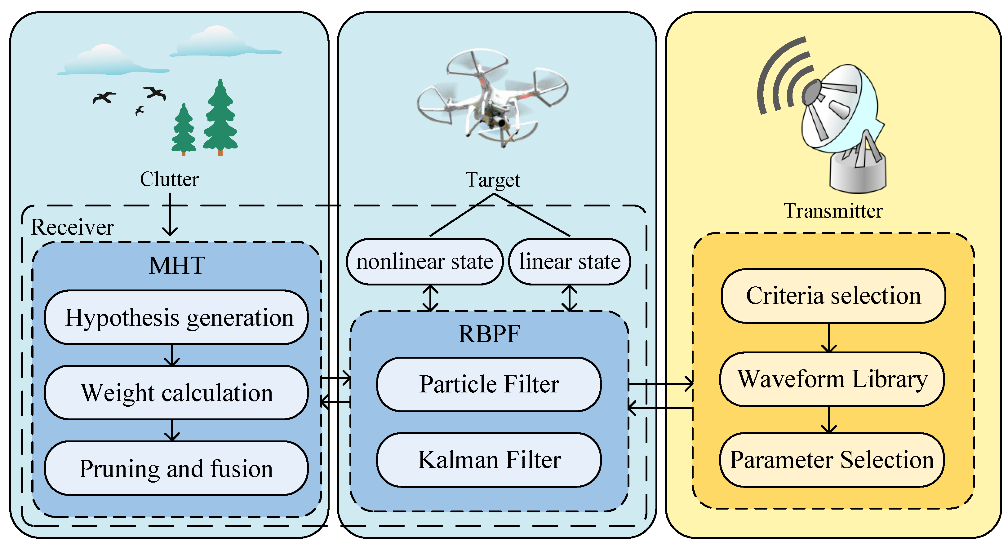
In this paper, we aim to formulate the IMCS mechanism so as to achieve the adaptive waveform selection. Herein, a complex three-dimensional hybrid model, combining linear and nonlinear states, is constructed to describe the high maneuverability of the target. Considering noise and clutter in a low-altitude environment, we try to integrate MHT into the RBPF framework to address interference and accurately estimate the target’s state. Furthermore, by using the IMCS method, we can select optimal transmitting waveform parameters from the waveform library, thereby improving the accuracy and robustness of tracking. Figure 1 illustrates the low-altitude maneuvering-target tracking process of a radar system.
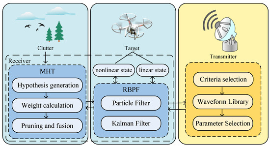
Figure 1.
Low-altitude maneuvering-target tracking process of a radar system.
2. System Overview
The radar receiver uses the MHT-RBPF algorithm to estimate the target states. Meanwhile, the radar transmitter selects the waveform parameters according to the feedback from the receiver and then emits waveforms. Firstly, the dynamic model of a low-altitude maneuvering target can be defined as
where is the target state vector at time instant k. and are the nonlinear and linear subsections, respectively. signifies the nonlinear state transition function. represents the transition matrix during the nonlinear state transforming, while is the linear transition matrix. is the measurement vector calculated by observing function . is the Gaussian process noise and is the measurement noise. The upper corner symbols n and l represent the nonlinear and linear components, respectively.
The target state vector includes the three-dimensional position and the velocity , i.e.,
where the updating of the x-axis position follows a nonlinear model, and the other state components are only linearly updated. Therefore, the nonlinear filter and linear filter can be applied for these state subspaces separately. is the measurement vector. The observing function has and
where represent the observing values for radial distance, radial velocity, azimuth angle, and elevation angle, respectively. is the position of radar receiver.
Suppose that the target is located at position and moving with the velocity ; then, the radar receiver could obtain the time delay and Doppler shift measurement .
The measurement error covariance matrix can be computed by using the Cramér–Rao Lower Bound (CRLB) [2], i.e.,
where is the transition matrix. According to [4], is the CRLB matrix of time delay and Doppler shift, which is also related to the signal-to-noise ratio (SNR) and the transmitted waveform parameters . Here, represents the simplified SNR of radar echo based on spatial geometry and distance attenuation [33], reflecting the variation in signal strength in propagation, caused by the changing distances between the target and receiver. represents the distance between the target and the radar receiver when the SNR is 0. t and r are the positions of the radar transmitter and receiver, respectively.
In fact, under a high-SNR condition, the Fisher Information Matrix (FIM), which is the inverse of the CRLB, usually depends on both the SNR and the second-order derivative of the ambiguity function, i.e.,
where and denote the actual time delay and Doppler shift, respectively. and denote the hypothesized time delay and Doppler shift, respectively. The ambiguity function is maximized when and .
As the sharpness of the ambiguity function is determined by the transmitted waveform, both the FIM and CRLB matrices are inherently dependent on the waveform selection [4].
Here, we mainly consider the effect of waveform parameters and explore the role of adaptive waveform selection strategies to optimize the tracking performance. As only angles are influenced by SNR, rather than position and velocity, the measurement error covariance matrix associated with waveform parameters can be obtained by
where is the Gaussian pulse length, and is the frequency modulation rate that can be calculated by the sweep frequency and the effective pulse duration [2]. can be approximated by .
Noteworthily, the measurement error covariance is evidently influenced by the pulse length and the frequency sweep . Therefore, the radar system can alleviate the measurement error and improve the tracking accuracy by building a waveform library and selecting optimal parameters. This adaptive waveform selection strategy is the key component to improve the overall performance.
3. Low-Altitude Maneuvering-Target Tracking in Clutter
To address low-altitude maneuvering target tracking, we focus on two primary issues, i.e., the accuracy problem caused by clutter and noise, and the complexity problem arising from the mixed state of the target model. As known, the MHT algorithm utilizes the hypothesis-based idea to generate multiple possible target trajectories. We apply this idea to deal with false measurements caused by clutter. In addition, the RBPF algorithm is used to tackle the complexity problem arising from the mixed state, e.g., (1) contains a linear sub-structure which can be leveraged to improve state estimation, as below:
where the linear component can be separated from the high-dimensional state space. It is analytically tractable and can be estimated using the KF. The remaining nonlinear component is processed using PF. By separating the linear state from the high-dimensional mixed-state space, particles are constrained to a lower-dimensional nonlinear state space. Furthermore, we integrate the MHT algorithm into the RBPF framework. The nonlinear component density is approximated using the standard PF. The MHT–RBPF algorithm is summarized in Algorithm 1.
| Algorithm 1 MHT–RBPF algorithm |
| Input: The state estimation and the covariance ,, posterior probability at time k-1. Output: The state estimation and the covariance ,, posterior probability at time k.
|
The specific steps of the MHT–RBPF algorithm are listed as follows:
- (1)
- PF prediction for the nonlinear state
Based on the state estimation and its covariance , obtained from the dynamic hybrid model, new particles for PF can be predicted by
The predicted nonlinear state has
where N is the number of particles;
- (2)
- KF prediction for the linear state
The prediction of linear states and its error covariance at time instant k can be calculated by
where .
Unlike traditional KF, it is more appropriate to regard the updating step as a correction of actual measurement by utilizing the information obtained from the prediction of nonlinear state variables [25]. This distinction arises from the fact that (1) clearly shows the nonlinear state variable indeed carrying the information of the linear state variable, which also indicates the nonlinear and linear state variables’ interacting with each other during the prediction process. and are the process variables reflecting the interaction between the nonlinear and linear states, and also demonstrate the influence between each other during the prediction step;
- (3)
- Acquisition of observation data
The predicted measurement can be calculated by
The detection probability of target is often less than 1 due to the interference and unwanted false-alarm measurements introduced by clutter, i.e.,
where is the false-alarm probability. Along with the genuine measurements corresponding to the target (if it is detected), the receiver also picks up unwanted false measurements due to the presence of clutter. According to [2], the resulting false alarms are assumed to be uniformly spatially distributed over the measurement space and independent over time. A Poisson distribution is used to model the number of false alarms, where the probability mass function of the false alarms in a volume is given by [34,35,36,37]
Here, the volume of the validation region is and is the clutter density.
In fact, the clutter along with the real measurement of target form the total observations in the received echo, i.e.,
- (4)
- Hypothesis generation
Hypothetical branches are generated based on the current measurement data, and each branch represents a possible target measurement association, where they also denote the target or clutter, i.e.,
For each hypothesis, the PF and KF are used to estimate the target state by steps (5)–(8);
- (5)
- Normalizing importance weights
Suppose that the importance distribution depends only on the target state and measurements at the previous time; the normalizing importance weights can be calculated by
The resampling process is conceptually similar to that of data association. The importance weights serve as the correlation probabilities, both measuring the degree of matching between the measurement data and the state estimation. This process not only mitigates the particles’ divergence but also reduces some clutter interference, thereby improving overall performance.
Specifically, the association probability can be modeled by Gaussian distribution, i.e.,
where is the residual of the i-th particle’s predicted measurement , i.e.,
- (6)
- PF measurement updating
By the resampling operation, the particles’ distribution can be approximated by each particle’s weight, i.e.,
- (7)
- Kalman state updating
- (8)
- Updating the array size
Since the amount of clutter generated from the Poisson distribution also varies at each time instant, the sizes of all resulting arrays need to be updated;
- (9)
- Calculating the association probability and updating hypothesis weights
The association probability between each hypothesis and target’s state prediction has
Then, the weight for each hypothesis is updated based on the association probability and prior probability. It is calculated by the Bayes formula, i.e.,
where is the prior probability;
- (10)
- Hypotheses pruning
The hypotheses are pruned according to these weights, and then the most likely hypotheses can be retained by directly sorting and selecting L hypotheses with the highest weight;
- (11)
- Hypotheses fusion
The hypotheses after pruning are fused according to weights. Firstly, the selected L high weights are normalized by
Then, we calculate the weighted sum of the state vector and covariance matrix by
Finally, we calculate the total posterior probability. The total posterior probability is deemed as the sum of posterior probabilities of all hypotheses by
According to te steps above, the low-altitude maneuvering target can be accurately tracked.
4. Adaptive Waveform Selection Mechanism and Discussion
4.1. Interacting Multiple-Criterion Selection Method
The IMM algorithm is used to estimate the state of the target with diverse models and noise characteristics. In our study, we focus on the waveform selection process among different criteria and varying cost functions, further presenting the interacting multiple criteria selection (IMCS) method. After completing the target state estimation at each time instant, the criterion selection process is performed. These detailed steps are listed as follows:
- (1)
- Initializing the weights
Each waveform selection criterion is assigned an initial weight, which represents the prior probability. The transition probabilities between each criterion are set and then formulate a transition matrix ;
- (2)
- Predict model probability
Given that there are L criteria, the prediction probability of each criterion is calculated based on the transition probability and prior probability,
where represents the transition probability from the criterion j to i in the transition probability matrix . is the effective probability of criterion j at time instant k;
- (3)
- Measurement of target
The transmitting waveform parameters are selected based on various criteria, and the target’s states are predicted in one step. The predicted measurements can be obtained by
- (4)
- Calculating the likelihood probability
For each criterion, the corresponding likelihood probability is calculated by comparing the predicted value with the expected output. The likelihood probability for the i-th criterion can be calculated by
where represents the residual error between the true measurement value and the predicted measurement:
- (5)
- Updating weights
The weight of each criterion can be updated based on the calculated likelihood probabilities and predicted probabilities, which is also the posterior probability, as follows:
- (6)
- Selecting the optimal criterion
The criterion with the highest probability is selected as the optimal one, and its parameter selection results are applied to target tracking at the next time;
- (7)
- Update the effective probability
4.2. Waveform Selection Criteria
As discussed in Section 2, the measurement error covariance matrix is dependent on the waveform parameters . As shown in Section 3, both the error covariance matrix and the residual covariance matrix are functions of . This establishes the foundation for the subsequent optimization methods in waveform parameter selection. First, we need to predict these relevant matrices at time instant using the aforementioned algorithm. Next, we discuss the criteria for waveform selection.
4.2.1. Max-Q Criterion
The Q-learning method updates the Q-table by calculating the expected return of actions at each time instant, ultimately identifying the optimal path to complete the task. The Q-value, which reflects cumulative discounted rewards, is derived from real-time rewards and potential future rewards. In the waveform selection process, the Q-value represents the expected return from selecting a particular waveform [33,38]. This paper discusses the Max-Q criterion, which is grounded in the principles of Q-learning for selecting waveform parameters.
where denotes the learning rate and represents the discount factor. As shown in (34), the new Q-value contains the value of current time instant and the rewards obtained from the currently selected waveform parameters. A higher Q-value indicates greater returns from selecting these parameters and improved tracking performance.
The real-time reward is represented as
where represents entropy state and measures the uncertainty in the state estimate. It can be calculated using the estimated error covariance :
According to (35), the prediction reward is computed based on the prediction error covariance matrix, and Q-values for each set of parameters are updated accordingly. The parameters that yield the highest Q-value are selected as the optimal transmitting waveform parameters for the next time instant. Thus, the Max-Q criterion can be defined as
where indicates the pre-set waveform library.
4.2.2. Minimum Mean Square Error Criterion
The Min-MSE criterion selects the optimal waveform parameters by minimizing the mean square error (MSE) of target state estimation. It is evident that this criterion aims to reduce the state estimation error. Thus, the criterion can be expressed as
whereas
Therefore, the criterion can be described as
4.2.3. Maximum Mutual Information Criterion
Based on the information theory, the mutual information (MI) between the state prediction and measurements indicates the degree of certainty in state estimation. Greater mutual information signifies a more accurate estimation and better target-tracking performance. Therefore, the adaptive waveform selection method under the Max-MI criterion can be described as [33,39]
whereas
Similar to the Min-MSE criterion, the Max-MI criterion can be expressed as minimizing the determinant of estimated error covariance matrix, i.e.,
4.2.4. Minimum Validation Gate Volume Criterion
Based on the measurements, the Min-Gate criterion enhances tracking performance by controlling the volume of the validation gate [40,41]. This criterion can be described as
The IMCS method utilizing the four criteria above can be summarized as in Algorithm 2.
| Algorithm 2 Interacting multiple-criterion selection method |
| Input: The effective probability of criterion i at time instant k, transition probability matrix . Input: Selected waveform parameters, .
|
5. Simulations and Analysis
In this section, we consider a radar system located at (0, 0, 0) with both transmitter and receiver together to track a maneuvering target. Here, we focus on a special three-dimensional low-altitude environment. The target’s triangular model is described in Section 2.
The initial state vector of target is given by
The initial-state estimation error covariance matrix is
Suppose that the radar transmits Gaussian linear frequency modulation (LFM) pulses with a transmission frequency of and pulse repetition interval of s [2].
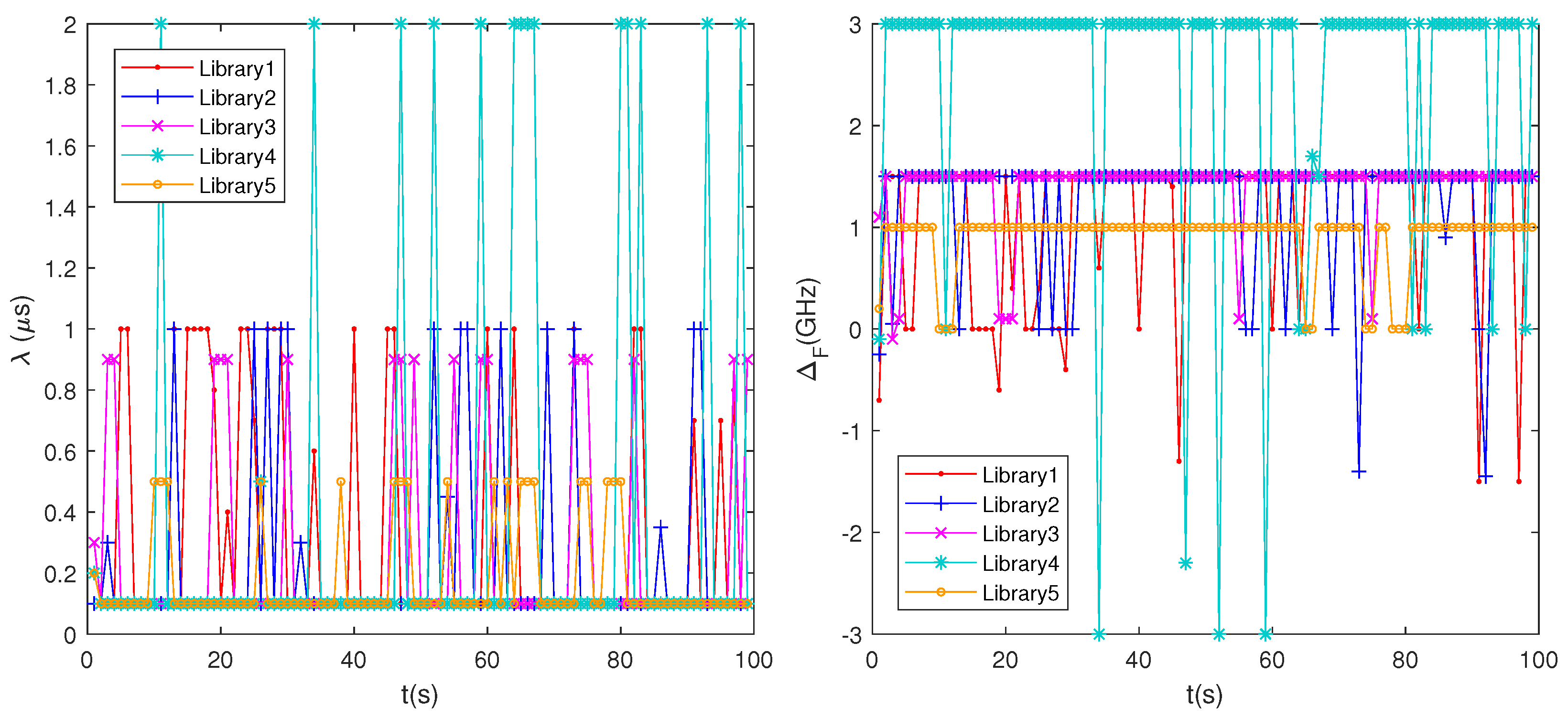
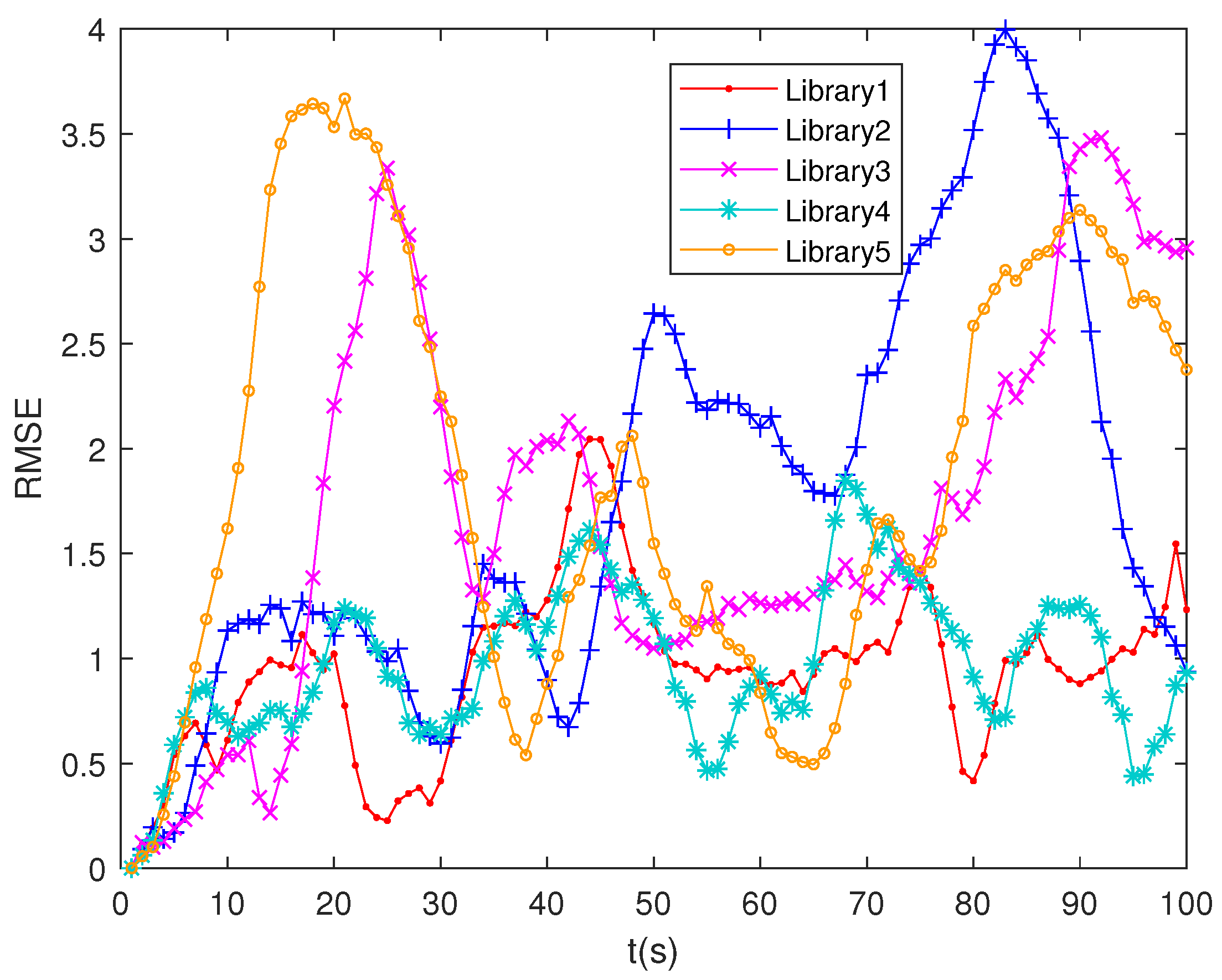
Firstly, according to the relationship between measurement error and waveform parameters discussed in Section 2, the waveform library is formulated by using pulse lengths and sweep frequencies. Here, we initially set the waveform parameter range and interval according to [2,33]. Then, we select parameters and conduct a series of comparisons to analyze their impact on tracking performance. Figure 2 and Figure 3 show the parameter selection process and the root mean square error (RMSE) of tracking when using different waveform libraries, respectively. (Library 1: , ; Library 2: , ; Library 3: , ; Library 4: , ; Library 5: , ).
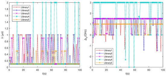
Figure 2.
The selection results of different parameter ranges and intervals.
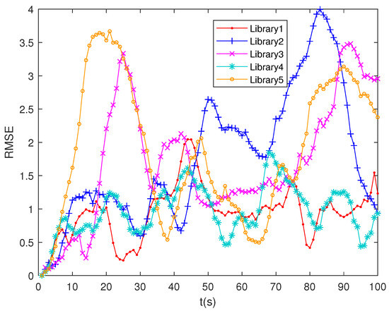
Figure 3.
RMSEs from the selection of different waveform libraries.
With the selected range of parameters increasing, the tracking error decreases, but the computational load increases. The interval has a relatively fixed optimal value. Ultimately, by considering both the tracking performance and computational efficiency, we determine an optimal waveform library to maximize tracking performance while balancing computational efficiency.
Here, the SNR at time instant k is modeled as with m. The probability of false alarms is , and the threshold corresponding to the gate probability is .
Then, the four waveform selection criteria mentioned in Section 4 are incorporated within IMCS models with initial probability 1/4. The criterion transition matrix is
Furthermore, the root mean square error (RMSE) and average RMSE (ARMSE) are used as indicators to evaluate the performance of proposed filtering algorithms and various waveform selection criteria, i.e.,
where , , etc., represent the true target states, while , , etc., denote the estimated ones. The ARMSE of the position estimation can be calculated by
Similarly, the ARMSE of other state components can also be obtained.
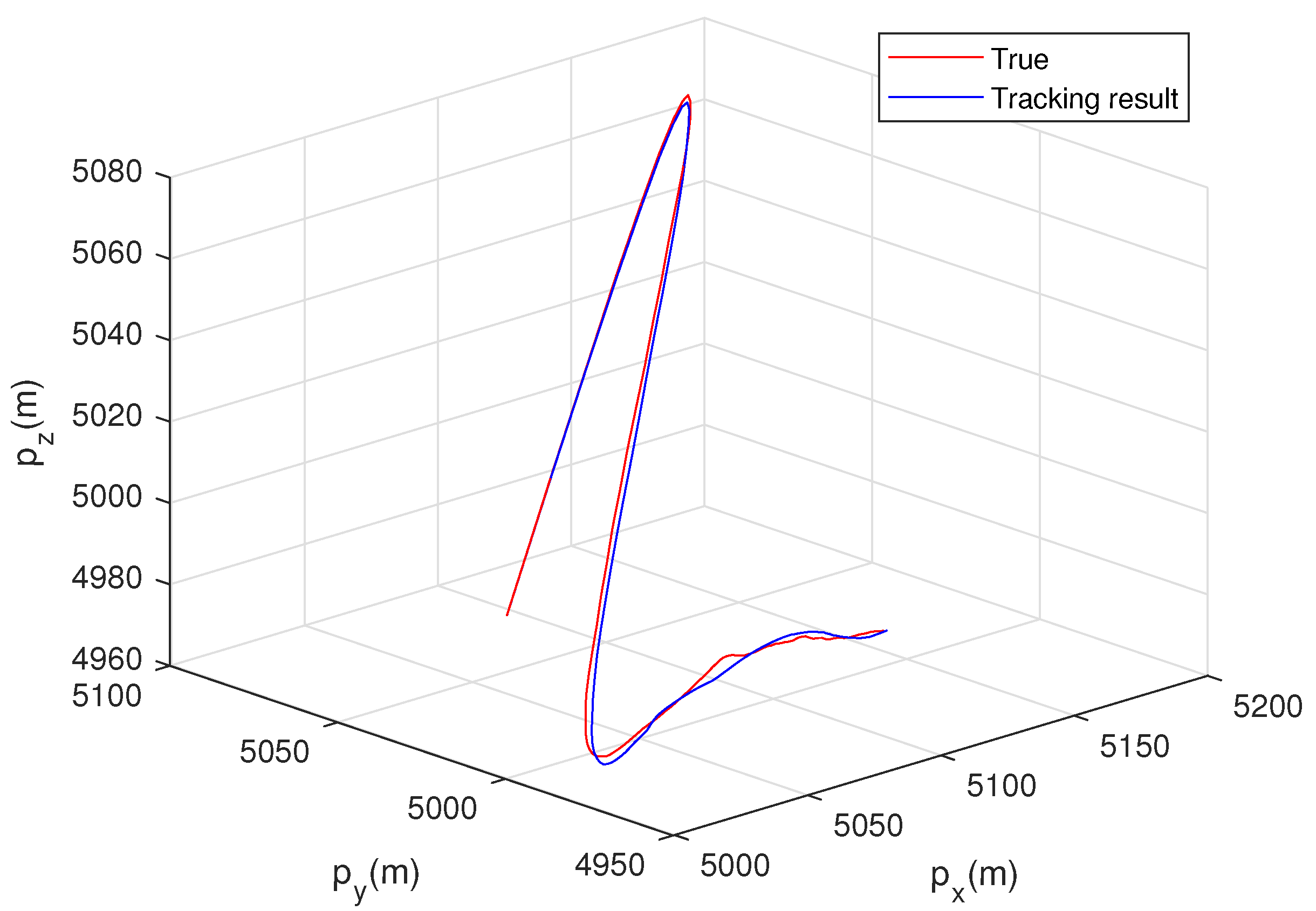
We firstly track a maneuvering target in low-altitude clutter using the MHT–RBPF algorithm and IMCS method for waveform selection. Figure 4 shows the target trajectory obtained by the proposed algorithms.
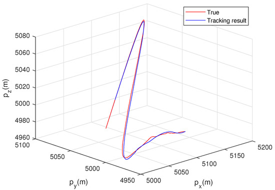
Figure 4.
Tracking result using the IMCS–MHT–RBPF algorithm.
Suppose that the target’s x-axis position follows a nonlinear model with the arctangent transition function; the nonlinear state, which carries information about the linear-state variable discussed in Section 2, has
Other state components adhere to a linear model, i.e.,
It can be seen from Figure 4 that the target exhibits maneuvering movement in three-dimensional space. The target’s dynamics can be divided into three stages, i.e., ascent, descent, and small fluctuations with turns. The target ascends rapidly from to . Between and , the target decelerates and descends. During the interval to , it performs slow, small undulating movements and turns. The turning occurs due to changing in the velocity direction. It is evident that the proposed algorithm effectively estimates the target trajectory. Tracking performance is specifically evaluated using the RMSE and ARMSE metrics.
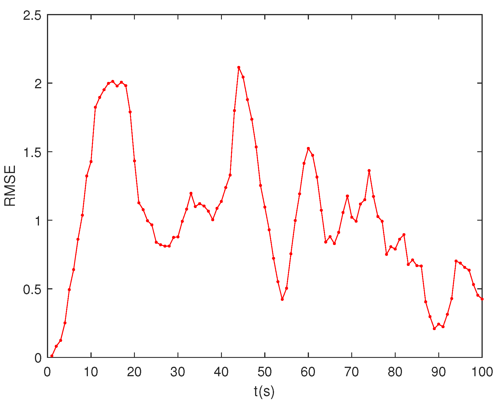
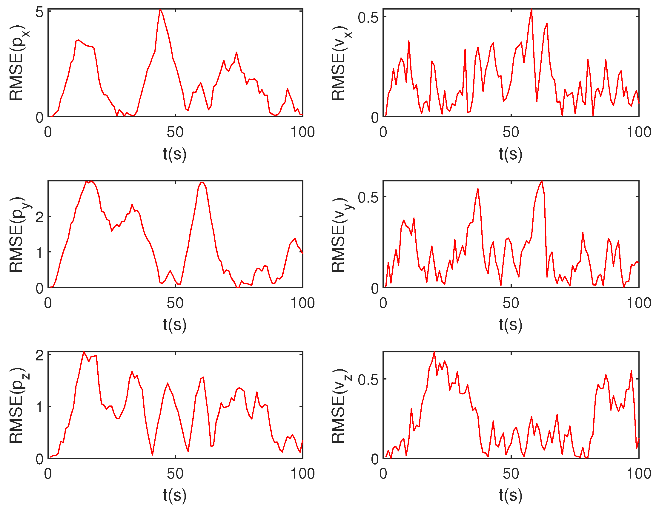
As shown in Figure 5 and Figure 6, the RMSE values during these time periods exhibit varying degrees of increase. Notably, increases in RMSE occur around , , and , coinciding with target state transitions. The MHT–RBPF algorithm and IMCS method keep the RMSE below 2.2. Additionally, Figure 6 shows that RMSE values for each state component remain within a small range. Specifically, the RMSE for the position component is approximately 2, while that for the velocity component remains below 0.5. Data from Table 1 indicate that the ARMSE for position estimation is about 1.7, and, for speed estimation, it is about 0.24. Therefore, the proposed algorithm demonstrates low error and excellent tracking performance.
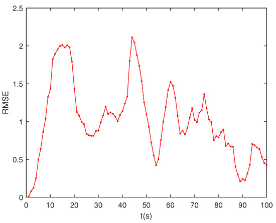
Figure 5.
RMSE for the IMCS–MHT–RBPF algorithm.
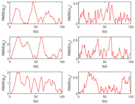
Figure 6.
RMSEs of each target state component for the IMCS–MHT–RBPF algorithm.

Table 1.
ARMSE for the IMCS–MHT–RBPF algorithm.
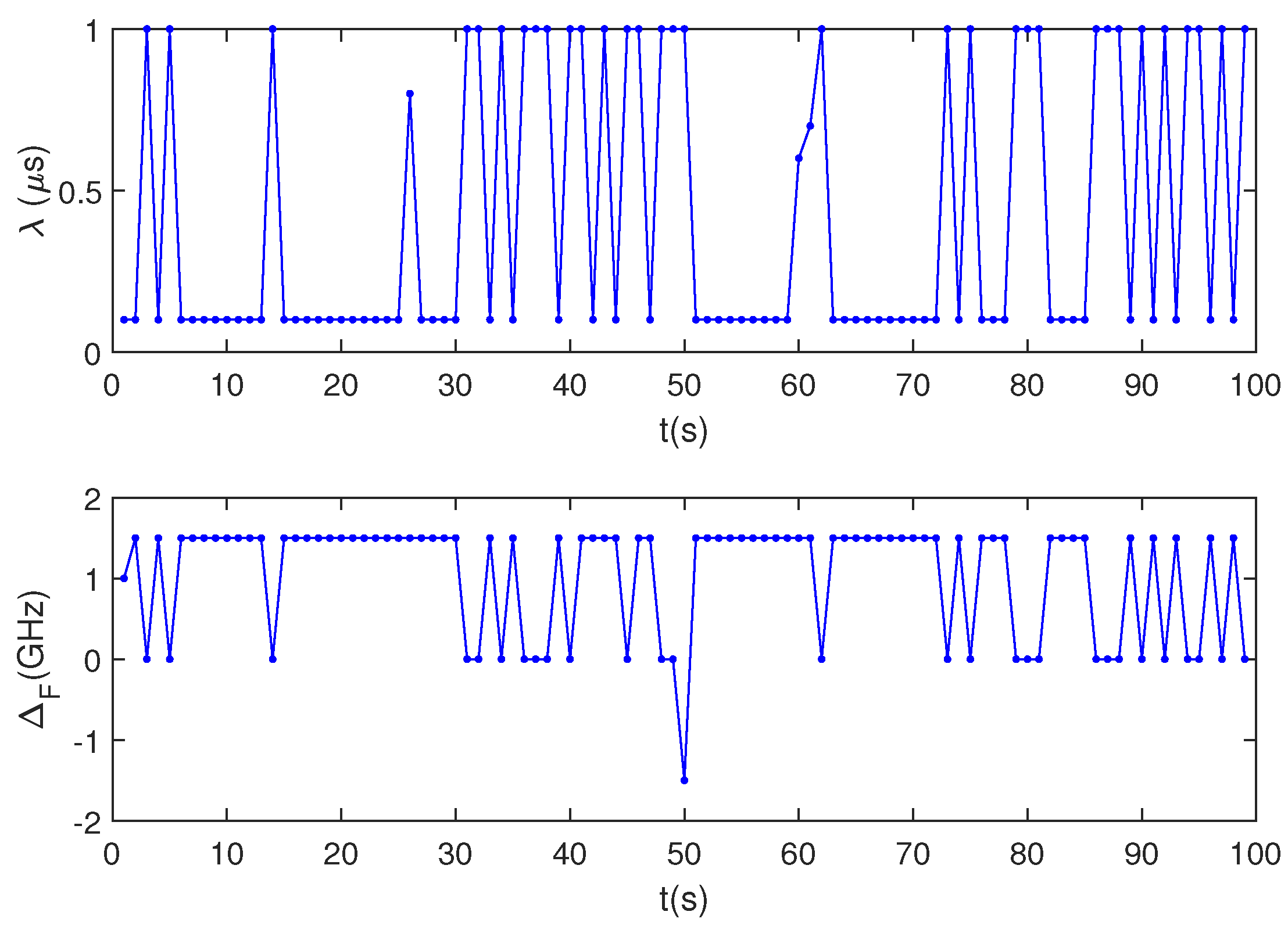
As illustrated in Figure 7, these parameters of waveform transmission are continuously adjusted, corresponding to the varying conditions. Figure 8 shows the selection results of the IMCS method at each time instant. The target-tracking process mainly utilizes the Max-Q and Max-MI criteria, with the occasional use of the Min-Gate criterion. This adaptive adjustment of waveform transmission enhances tracking accuracy.
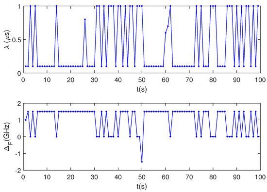
Figure 7.
Patterns of selected waveform parameters (Gaussian pulse length and sweep frequency).
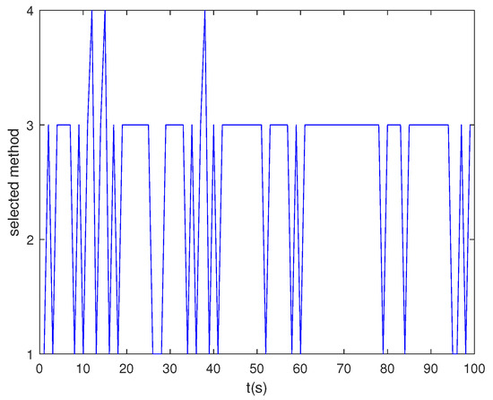
Figure 8.
Index of the selected criterion at each time instant. (1: Max-Q; 2: Min-MSE; 3: Max-MI; 4: Min-Gate).
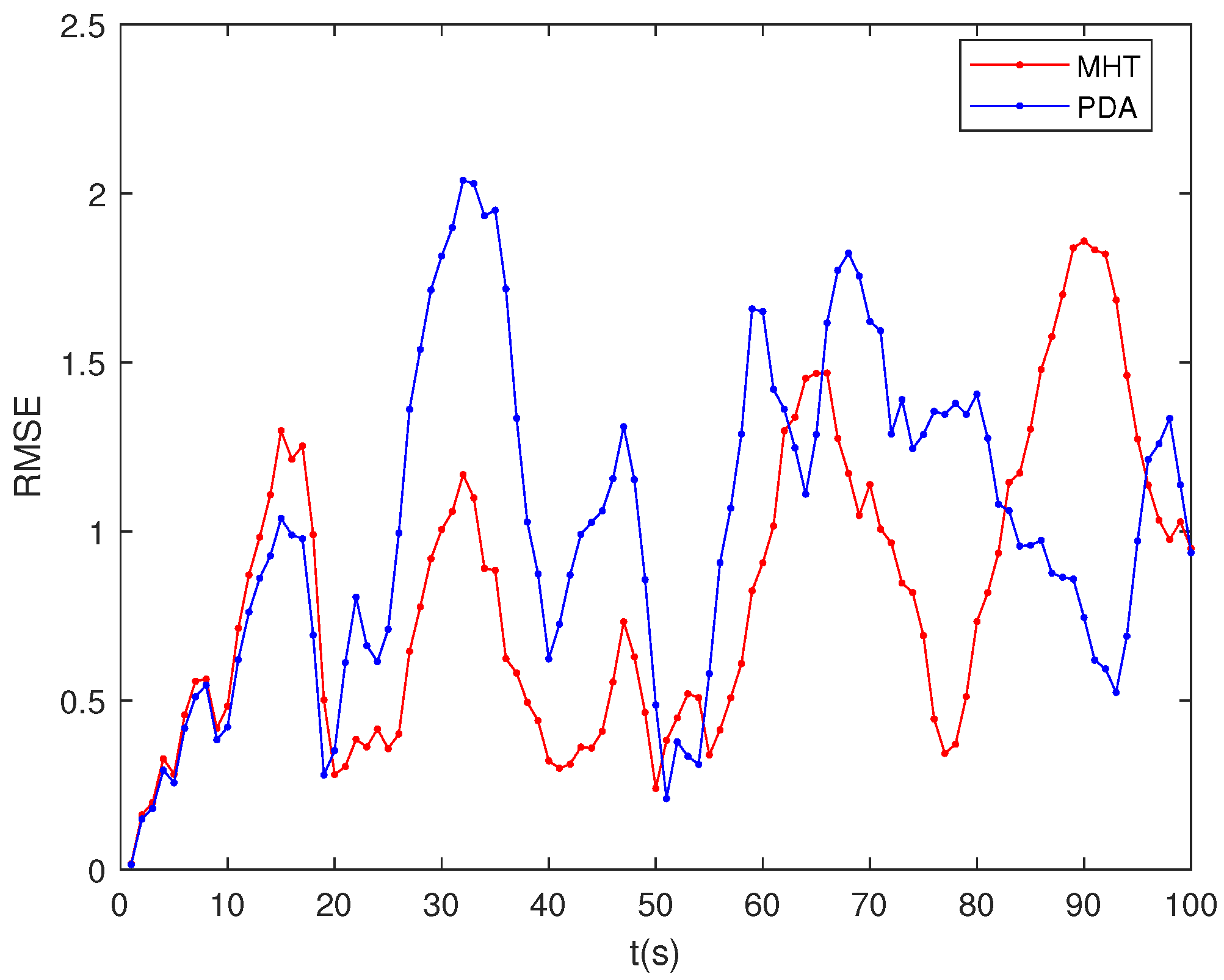
Next, the performance of the MHT algorithm is compared with that of the classical PDA algorithm under the same clutter conditions. Figure 9 presents the RMSE for state estimation. Table 2 provides a performance comparison of these two methods, including the ARMSE of state estimation, CPU time, and memory usage. When combined with the RBPF algorithm, the asymptotic time complexities of the MHT and PDA algorithms are and , respectively, while the asymptotic space complexities are and , respectively. The higher complexity of the MHT algorithm is attributed to the substantial computational load associated with multi-hypothesis state estimation.
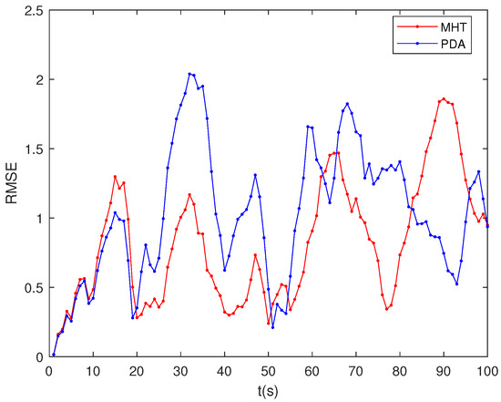
Figure 9.
RMSE of different clutter-processing methods for state estimation.

Table 2.
Performance comparison of different clutter-processing methods.
Through a series of Monte Carlo simulations, it is found that the MHT algorithm achieves lower tracking error and performs slightly better than the PDA. However, the computation time is significantly greater, and the asymptotic time and space complexity are also higher than those of the PDA. In other words, the MHT algorithm improves tracking performance at the cost of complexity. The PDA performs well in terms of speed with high computational efficiency, making it suitable for applications with demanding real-time requirements. The MHT algorithm has high robustness and scalability, but needs sufficient computing resources. By employing the MHT algorithm, we can analyze multiple potential measurement hypotheses, effectively associating and verifying data to distinguish target signals from clutter, thereby improving tracking accuracy and stability.
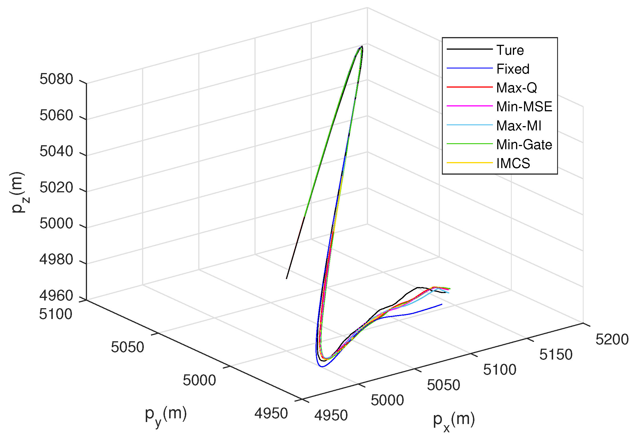
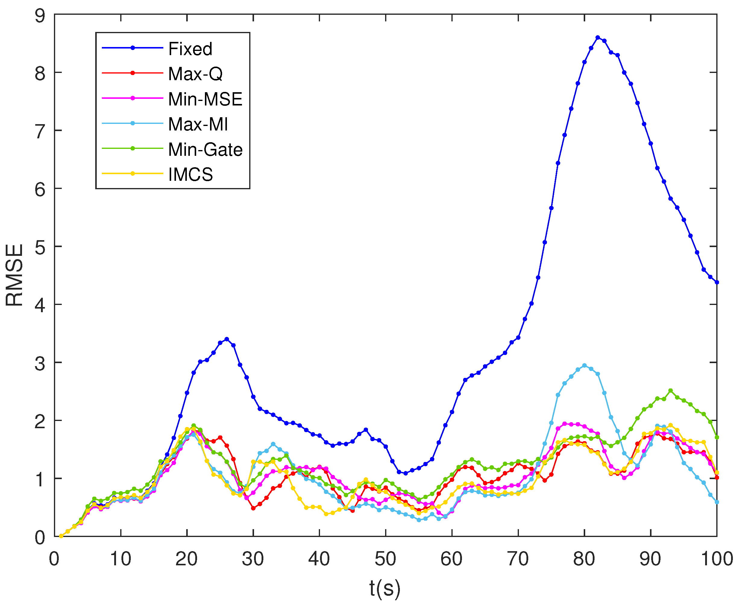
Next, we apply the IMCS method to select waveform parameters, compared with the fixed-waveform and single-waveform selection criteria. As illustrated in Figure 10 and Figure 11 as well as Table 3, it is evident that using a fixed waveform cannot adapt well to track the maneuvering target, resulting in large tracking error and poor adaptability. By adjusting waveforms using selection criteria, the tracking error can be significantly reduced, and tracking accuracy is improved, while the RMSE can be maintained below 2. Furthermore, by comparing the effective probability to choose a selection criterion, the RMSE of the IMCS method can be kept at a lower level than that of each single selection criterion, resulting in more stable error and better adaptability.
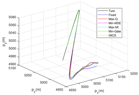
Figure 10.
Tracking results using different waveform selection criteria.
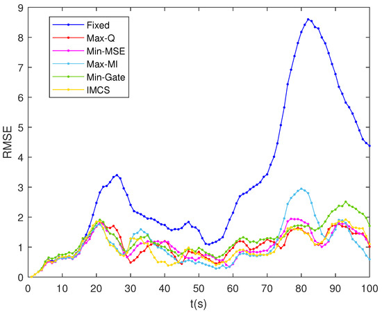
Figure 11.
RMSE of different waveform selection criteria.

Table 3.
ARMSE of different waveform selection criteria.
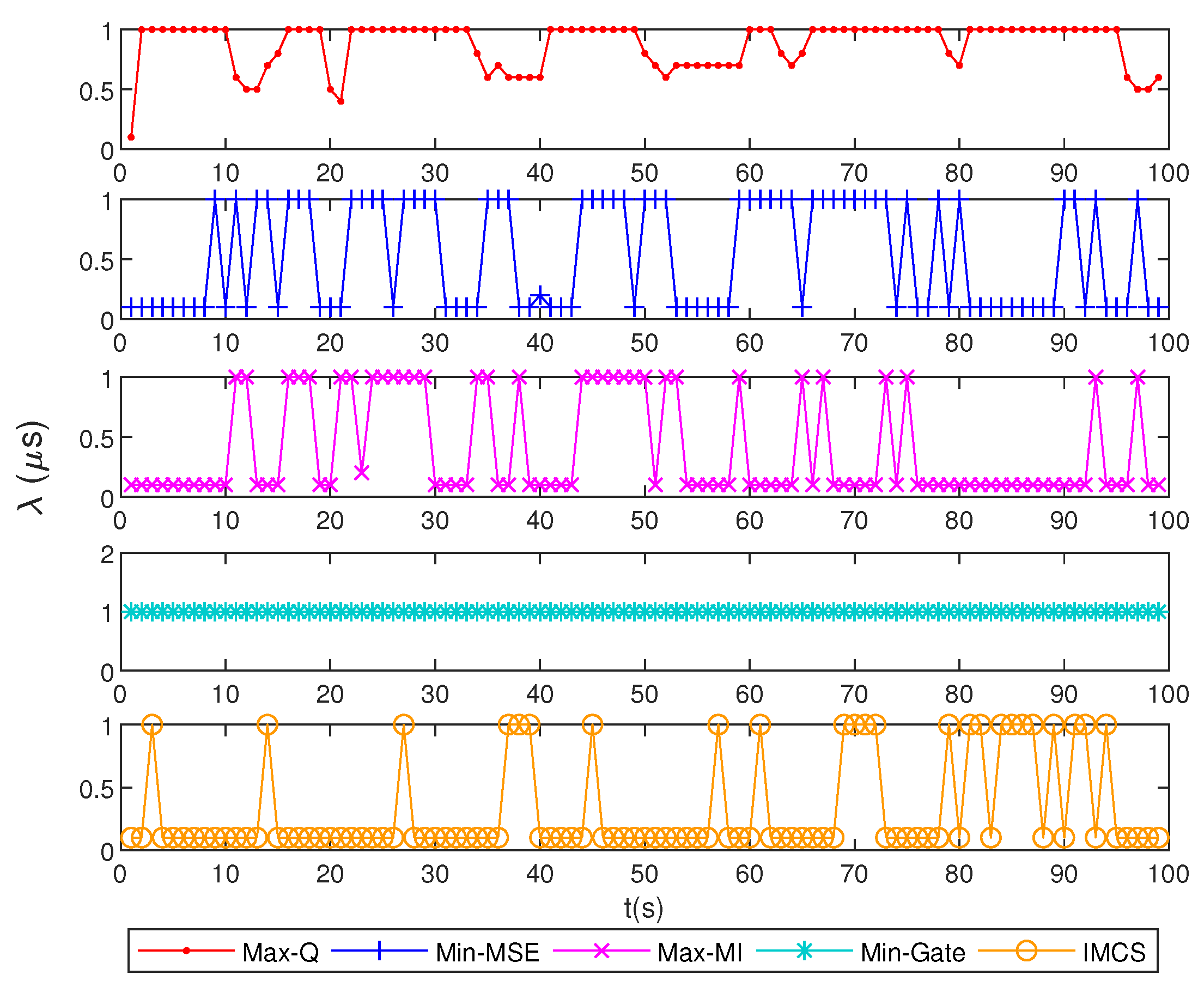
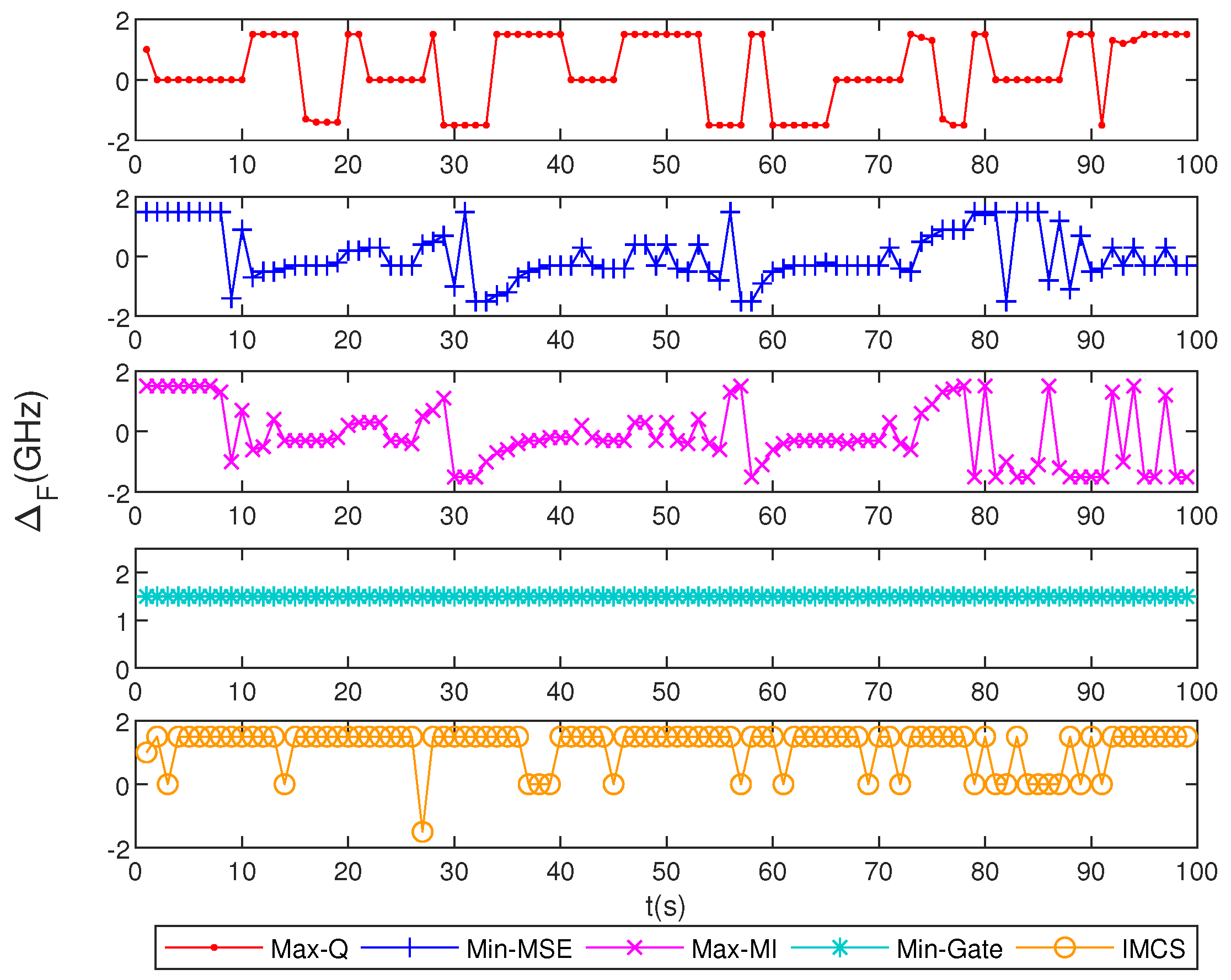
To effectively deal with noise, clutter, and the maneuvering states of the target, the radar must dynamically adjust its transmitted waveforms to enhance the tracking performance. Figure 12 and Figure 13 illustrate the parameter-selection process based on different waveform selection criteria at each time instant. Different criteria select waveform parameters based on varying cost functions. Due to their reliance on the estimation error covariance matrix, the waveform parameter selection processes of Min-MSE and Max-MI criteria are all similar. Min-Gate criterion hardly adjusts parameters, but it has relatively good tracking performance. This may be attributed to the Min-Gate criterion focusing on minimizing the validation gate volume, which ensures that the highly probable target measurements are considered. By constraining the gate size, it could reduce false associations and improve tracking accuracy, even without frequent parameter adjustments. In relatively stable scenarios, the Min-Gate criterion could lead to good performance without constantly updating parameters.
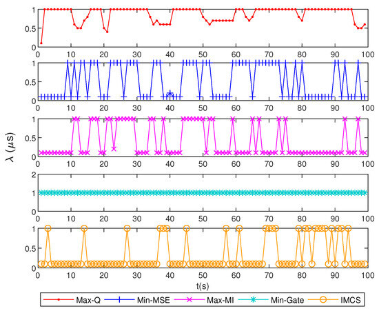
Figure 12.
Patterns of selected pulse lengths using different waveform selection criteria.
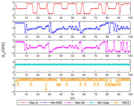
Figure 13.
Patterns of selected sweep frequencies using different waveform selection criteria.
Since the IMCS method involves traversing the waveform library and interactively selecting multiple criteria, it inevitably increases the computational load and and impacts its feasibility for real-time applications. The increasing complexity can be seen as a common challenge in cognitive radar systems, where adaptive and dynamic waveform selection strategies need to balance the performance and computational efficiency. However, due to the flexible nature of interacting multiple models, the algorithm allows for the addition or reduction of criteria based on specific requirements, which is crucial for different practical scenarios.
6. Conclusions
For low-altitude maneuvering-target tracking, a novel IMCS method based on an IMM framework and the MHT–RBPF algorithm has been proposed to reduce measurement errors and improve tracking performance. Therein, the principles of the MHT algorithm and RBPF algorithm are both adopted to estimate target states. The IMCS method adaptively selects transmitted waveform parameters and achieves a superior selection criterion. Simulation results demonstrate that the MHT–RBPF algorithm performs well for tracking a maneuvering target in low-altitude clutter. The IMCS method, by selecting the optimal criterion and parameters, could maintain the RMSE within a small range, which shows better performance than the fixed-waveform or single-waveform selection criteria. This adaptive waveform selection method significantly enhances both the accuracy and robustness of radar target tracking, providing a more effective solution for a dynamic and cluttered environment.
Author Contributions
Conceptualization, X.F. and Z.Z.; methodology, P.S.; software, L.Z.; validation, X.F., J.W. and Z.Z.; formal analysis, P.S.; investigation, X.F. and G.J.; resources, J.W.; data curation, P.S.; writing—original draft preparation, P.S.; writing—review and editing, X.F. and G.J.; visualization, P.S.; supervision, X.F.; project administration, Z.Z.; funding acquisition, Z.Z. All authors have read and agreed to the published version of the manuscript.
Funding
This document is a result of the research project funded by Major Scientific and Technological Innovation Projects of Shandong Province of China (Grants 2021ZLGX05 and 2022ZLGX04).
Data Availability Statement
The original contributions presented in the study are included in the article, further inquiries can be directed to the corresponding author.
Conflicts of Interest
The authors declare no conflicts of interest.
References
- Su, Y.; Cheng, T.; He, Z.; Li, X. Joint Waveform Control and Resource Optimization for Maneuvering Targets Tracking in Netted Colocated MIMO Radar Systems. IEEE Syst. J. 2022, 16, 3960–3971. [Google Scholar] [CrossRef]
- Nguyen, N.H.; Doğançay, K. Signal Processing for Multistatic Radar Systems: Adaptive Waveform Selection, Optimal Geometries and Pseudolinear Tracking Algorithms; Academic Press: Cambridge, MA, USA, 2019. [Google Scholar]
- Kershaw, D.J.; Evans, R.J. Optimal waveform selection for tracking systems. IEEE Trans. Inf. Theory 1994, 40, 1536–1550. [Google Scholar] [CrossRef]
- Nguyen, N.H.; Dogancay, K.; Davis, L.M. Adaptive waveform selection for multistatic target tracking. IEEE Trans. Aerosp. Electron. Syst. 2015, 51, 688–701. [Google Scholar] [CrossRef]
- Yang, Y.; Blum, R.S. MIMO radar waveform design based on mutual information and minimum mean-square error estimation. IEEE Trans. Aerosp. Electron. Syst. 2007, 43, 330–343. [Google Scholar] [CrossRef]
- Herbert, S.; Hopgood, J.R.; Mulgrew, B. MMSE Adaptive Waveform Design for Active Sensing with Applications to MIMO Radar. IEEE Trans. Signal Process. 2018, 66, 1361–1373. [Google Scholar] [CrossRef]
- Liu, Y.; Liao, G.; Xu, J.; Yang, Z.; Zhang, Y. Adaptive OFDM Integrated Radar and Communications Waveform Design Based on Information Theory. IEEE Commun. Lett. 2017, 21, 2174–2177. [Google Scholar] [CrossRef]
- Sun, J.; Wang, C.; Shi, Q.; Ren, W.; Yao, Z.; Yuan, N. Intelligent optimization methods of phase-modulation waveform. J. Syst. Eng. Electron. 2022, 33, 916–923. [Google Scholar] [CrossRef]
- Hu, J.; Wei, Z.; Li, Y.; Li, H.; Wu, J. Designing unimodular waveform (s) for MIMO radar by deep learning method. IEEE Trans. Aerosp. Electron. Syst. 2020, 57, 1184–1196. [Google Scholar] [CrossRef]
- Thornton, C.E.; Kozy, M.A.; Buehrer, R.M.; Martone, A.F.; Sherbondy, K.D. Deep Reinforcement Learning Control for Radar Detection and Tracking in Congested Spectral Environments. IEEE Trans. Cogn. Commun. Netw. 2020, 6, 1335–1349. [Google Scholar] [CrossRef]
- Thornton, C.E.; Buehrer, R.M.; Dhillon, H.S.; Martone, A.F. Universal Learning Waveform Selection Strategies for Adaptive Target Tracking. IEEE Trans. Aerosp. Electron. Syst. 2022, 58, 5798–5814. [Google Scholar] [CrossRef]
- Patrick, U.; Rao, S.K.; Jagan, B.O.L.; Rai, H.M.; Agarwal, S.; Pak, W. Radar-Based Target Tracking Using Deep Learning Approaches with Unscented Kalman Filter. Appl. Sci. 2024, 14, 8332. [Google Scholar] [CrossRef]
- Thornton, C.E.; Buehrer, R.M.; Martone, A.F. Constrained Contextual Bandit Learning for Adaptive Radar Waveform Selection. IEEE Trans. Aerosp. Electron. Syst. 2022, 58, 1133–1148. [Google Scholar] [CrossRef]
- Shi, C.; Wang, Y.; Salous, S.; Zhou, J.; Yan, J. Joint Transmit Resource Management and Waveform Selection Strategy for Target Tracking in Distributed Phased Array Radar Network. IEEE Trans. Aerosp. Electron. Syst. 2022, 58, 2762–2778. [Google Scholar] [CrossRef]
- Zheng, Z.; Li, W.; Zou, K. Airborne Radar Anti-Jamming Waveform Design Based on Deep Reinforcement Learning. Sensors 2022, 22, 8689. [Google Scholar] [CrossRef] [PubMed]
- Qin, J.; Zhu, M.; Pan, Z.; Li, Y.; Li, Y. Memory-based deep reinforcement learning for cognitive radar target tracking waveform resource management. IET Radar Sonar Navig. 2023, 17, 1822–1836. [Google Scholar] [CrossRef]
- Bar-Shalom, Y.; Li, X.R.; Kirubarajan, T. Estimation with Applications to Tracking and Navigation: Theory Algorithms and Software; John Wiley & Sons: Hoboken, NJ, USA, 2004. [Google Scholar]
- Ito, K.; Xiong, K. Gaussian filters for nonlinear filtering problems. IEEE Trans. Autom. Control 2000, 45, 910–927. [Google Scholar] [CrossRef]
- Zhu, B.; Chang, L.; Xu, J.; Zha, F.; Li, J. Huber-based adaptive unscented Kalman filter with non-Gaussian measurement noise. Circuits Syst. Signal Process. 2018, 37, 3842–3861. [Google Scholar] [CrossRef]
- Arasaratnam, I.; Haykin, S. Cubature kalman filters. IEEE Trans. Autom. Control 2009, 54, 1254–1269. [Google Scholar] [CrossRef]
- Wang, J.; Qin, Y.; Wang, H.; Li, X. Dynamic waveform selection for manoeuvering target tracking in clutter. IET Radar Sonar Navig. 2013, 7, 815–825. [Google Scholar] [CrossRef]
- Sira, S.P.; Li, Y.; Papandreou-Suppappola, A.; Morrell, D.; Cochran, D.; Rangaswamy, M. Waveform-agile sensing for tracking. IEEE Signal Process. Mag. 2009, 26, 53–64. [Google Scholar] [CrossRef]
- Li, Y.; Bian, C. Object Tracking in Satellite Videos: A Spatial-Temporal Regularized Correlation Filter Tracking Method with Interacting Multiple Model. IEEE Geosci. Remote Sens. Lett. 2022, 19, 6511105. [Google Scholar] [CrossRef]
- Qi, S.; Yao, P. Persistent Tracking of Maneuvering Target Using IMM Filter and DMPC by Initialization-Guided Game Approach. IEEE Syst. J. 2019, 13, 4442–4453. [Google Scholar] [CrossRef]
- Schon, T.; Gustafsson, F.; Nordlund, P.J. Marginalized particle filters for mixed linear/nonlinear state-space models. IEEE Trans. Signal Process. 2005, 53, 2279–2289. [Google Scholar] [CrossRef]
- Vitetta, G.M.; Sirignano, E.; Viesti, P.D.; Montorsi, F.; Sola, M. Marginalized Particle Filtering and Related Filtering Techniques as Message Passing. IEEE Trans. Signal Process. 2019, 67, 1522–1536. [Google Scholar] [CrossRef]
- Bar-Shalom, Y.; Daum, F.; Huang, J. The probabilistic data association filter. IEEE Control Syst. Mag. 2009, 29, 82–100. [Google Scholar]
- Zeng, T.; Zheng, L.; Li, Y.; Chen, X.; Long, T. Offline performance prediction of PDAF with Bayesian detection for tracking in clutter. IEEE Trans. Signal Process. 2012, 61, 770–781. [Google Scholar] [CrossRef]
- Huang, J.; Xie, J.; Zhang, H.; Li, Z.; Qi, C. A Novel Tracking Algorithm Based on Waveform Selection for Maneuvering Targets in Clutter. Circuits Syst. Signal Process. 2024, 43, 3160–3179. [Google Scholar] [CrossRef]
- Hong, S.M.; Evans, R.; Shin, H.S. Optimization of waveform and detection threshold for range and range-rate tracking in clutter. IEEE Trans. Aerosp. Electron. Syst. 2005, 41, 17–33. [Google Scholar] [CrossRef]
- Sira, S.P.; Papandreou-Suppappola, A.; Morrell, D. Dynamic Configuration of Time-Varying Waveforms for Agile Sensing and Tracking in Clutter. IEEE Trans. Signal Process. 2007, 55, 3207–3217. [Google Scholar] [CrossRef]
- Coraluppi, S.P.; Carthel, C.A. Multiple-hypothesis tracking for targets producing multiple measurements. IEEE Trans. Aerosp. Electron. Syst. 2018, 54, 1485–1498. [Google Scholar] [CrossRef]
- Zhu, P.; Liang, J.; Luo, Z.; Shen, X. Cognitive Radar Target Tracking Using Intelligent Waveforms Based on Reinforcement Learning. IEEE Trans. Geosci. Remote. Sens. 2023, 61, 5107315. [Google Scholar] [CrossRef]
- Mbouombouo Mboungam, A.H.; Zhi, Y.; Fonzeu Monguen, C.K. Clutter Map Constant False Alarm Rate Mixed with the Gabor Transform for Target Detection via Monte Carlo Simulation. Appl. Sci. 2024, 14, 2967. [Google Scholar] [CrossRef]
- Liu, B.; Tharmarasa, R.; Jassemi, R.; Brown, D.; Kirubarajan, T. Extended Target Tracking with Multipath Detections, Terrain-Constrained Motion Model and Clutter. IEEE Trans. Intell. Transp. Syst. 2021, 22, 7056–7072. [Google Scholar] [CrossRef]
- Tian, X.; Liu, J.; Mallick, M.; Wang, J.; Ji, X.; Su, L.; Si, J. A Novel AD-PDA-BACF Algorithm for Real-Time Moving Target Shadow Tracking Using ViSAR Imagery. IEEE Trans. Geosci. Remote Sens. 2023, 61, 5208117. [Google Scholar] [CrossRef]
- Bar-Shalom, Y.; Li, X.R. Multitarget-Multisensor Tracking: Principles and Techniques; YBS Publishing: Storrs, CT, USA, 1995. [Google Scholar]
- Feng, X.; Sun, P.; Liang, M.; Wang, X.; Zhao, Z.; Zhou, Z. Radar Waveform Selection for Maneuvering Target Tracking in Clutter with PDA-RBPF and Max-Q-Based Criterion. Remote Sens. 2024, 16, 1925. [Google Scholar] [CrossRef]
- Roman, J.; Garnham, J.; Antonik, P. Information Theoretic Criterion for Waveform Selection. In Proceedings of the Fourth IEEE Workshop on Sensor Array and Multichannel Processing, Waltham, MA, USA, 12–14 July 2006; pp. 444–448. [Google Scholar] [CrossRef]
- Lee, G.; Kwon, J.; Kwak, N.; Yang, E. Robust measurement validation for radar target tracking using prior information. IET Radar Sonar Navig. 2019, 13, 1842–1849. [Google Scholar] [CrossRef]
- Hurtado, M.; Zhao, T.; Nehorai, A. Adaptive Polarized Waveform Design for Target Tracking Based on Sequential Bayesian Inference. IEEE Trans. Signal Process. 2008, 56, 1120–1133. [Google Scholar] [CrossRef]
Disclaimer/Publisher’s Note: The statements, opinions and data contained in all publications are solely those of the individual author(s) and contributor(s) and not of MDPI and/or the editor(s). MDPI and/or the editor(s) disclaim responsibility for any injury to people or property resulting from any ideas, methods, instructions or products referred to in the content. |
© 2024 by the authors. Licensee MDPI, Basel, Switzerland. This article is an open access article distributed under the terms and conditions of the Creative Commons Attribution (CC BY) license (https://creativecommons.org/licenses/by/4.0/).

