Abstract
The Norwegian Environment Agency is responsible for updating a map of undisturbed nature, which is performed every five years based on aerial photos. Some of the aerial photos are already up to five years old when a new version of the map of undisturbed nature is published. Thus, several new nature interventions may have been missed. To address this issue, the timeliness and mapping accuracy were improved by integrating Sentinel-2 satellite imagery for the detection of new roads across Norway. The focus on new roads was due to the fact that most new nature interventions include the construction of new roads. The proposed methodology is based on applying U-Net on all the available summer images with less than 10% cloud cover over a five-year period, with an aggregation step to summarize the predictions. The observed detection rate was 98%. Post-processing steps reduced the false positive rate to 46%. However, as the false positive rate was still substantial, the manual verification of the predicted new roads was needed. The false negative rate was low, except in areas without vegetation.
1. Introduction
The Norwegian Environment Agency is responsible for updating a map of undisturbed nature, which is performed every five years. As of 2018, 44% of Norway’s land area, excluding Svalbard, was undisturbed, meaning that there were no heavy technical interventions less than 1 km from any of this area. The area of undisturbed nature is slowly being reduced from 46% in 1988; thus, 2% of Norway’s land area has changed from undisturbed to disturbed in the last 30 years.
The every-five years update cycle is linked to the frequency of aerial photography in Norway, which is completed within five years before a new cycle is started. Each year, all the aerial photos captured that year are used to update the official base maps with new roads, buildings, power lines, etc. Then, after five years, all new heavy interventions, such as roads, railways, built-up areas, ski lifts, power lines, hydropower dams and wind power turbines are mapped for all of Norway. 1 km buffer zones for all these may then be used to find the intersection with the previous mapping of the areas of undisturbed nature. The intersection is subtracted to produce an updated map of undisturbed nature.
One obvious drawback with this method is that some of the aerial photos are already up to five years old when a new version of the map of undisturbed nature is published. Thus, several new nature interventions may have been missed, and the total area of undisturbed nature is slightly overestimated. Therefore, other sources for the mapping of new nature interventions were sought.
Undisturbed nature is one out of eight environment indicators for the national environmental goal of ensuring that ecosystems have good conditions and can deliver ecosystem services. The loss of undisturbed nature has three major components:
- Landscape fragmentation, i.e., a large area is divided by, e.g., a new road or power line;
- The loss of area, e.g., by city expansion or by building a new windmill park;
- The loss of area of high conservation value.
Jaeger [1] proposes three new measures of landscape fragmentation: the degree of landscape division, the splitting index, and the effective mesh size, and compares them with five existing fragmentation indices. Torres et al. [2] analyzed habitat loss and deterioration for birds and mammals in Spain due to transportation infrastructure development. Sverdrup-Thygeson et al. [3] analyzed a network of 9400 plots in productive forests in Norway to assess if current regulations target forests of high conservation value, and concluded that forest conservation must be improved for these areas.
Satellite remote sensing provides daily to monthly coverage, albeit at a coarser resolution than aerial photography. Depending on the size of the objects one wishes to monitor, satellite imagery may be a favorable alternative in several environmental monitoring applications. Lehmler et al. [4] used a combination of Sentinel-2, Sentinel-1, and Palsar-2 satellite data in a random forest classifier for the estimation of urban green volume. Deche et al. [5] used aerial photographs (1972), Landsat (1980, 2000), and SPOT-5 (2016) satellite images in a manual workflow for the estimation of land use and land cover changes between 1972 and 2016 in a study area in Ethiopia. Demichelis et al. [6] combined land cover classification of Sentinel-2 satellite imagery with an analysis of local people’s interaction with the landscape in a protected area in Gabon, and suggested designing conservation actions at the local scale.
Brandão and Souza [7] used Landsat images for the manual vectorization of unofficial roads in the Brazilian Amazon. High visual contrast was obtained by using false color images, with band 5 (shortwave infrared, 1650 nm), band 4 (near-infrared, 830 nm), and band 3 (red, 660 nm) displayed as red, green, and blue, respectively. This approach showed that unofficial roads are built at a rate of 14.5 km per 10,000 km2 per year in the study area in the Amazon, and that more than 3500 km of unofficial roads have been built in protected areas.
Ahmed et al. [8] used a pixel-based spectral band index followed by unsupervised segmentation to extract roads from Sentinel-2 images of Lahore, Pakistan and Richmond, Virginia, USA. The spectral band index was tailored to detecting asphalt surfaces. This method worked well in areas with high vegetation and in barren lands, but had problems near buildings and concrete structures. However, we were not interested in only asphalt roads; most of the roads we were interested in were gravel roads, with spectral signatures that could be similar to vegetation-free rock surfaces in the terrain.
Ayala et al. [9] combined super-resolution and semantic segmentation in a deep neural network to extract roads at 2.5 m resolution from Sentinel-2 data. This deep neural network was a modification of the popular U-Net [10], and Ayala et al. [9] obtained better results than with an ordinary U-Net on 10 m resolution Sentinel-2 data. However, the results were obtained for urban areas in Spain. In contrast, many forest roads in Norway are not as easily detected in Sentinel-2 imagery due to their less distinct appearances.
Sirko et al. [11] combined 32 Sentinel-2 images at 10 m resolution of the same area to achieve 50 cm super-resolution, for the purpose of building and road detection. Nevertheless, this technique might encounter difficulties with newly constructed roads that are only visible in some of the images, a common scenario under the frequently cloudy conditions in Norway. Jia et al. [12] used settlement information in a modified U-Net to improve rural road extraction from Sentinel-2 images in 2.5 m super-resolution. However, this method fell short in areas where new forest roads often lie far from established settlements.
The Sentinel-2 satellites of the European Space Agency capture multispectral optical images weekly at 10 m resolution in four bands, 20 m resolution in six bands, and 60 m resolution in three bands. New roads are usually visible in these images (Figure 1), especially in forests where the contrast to existing vegetation is high in, e.g., the near-infrared band. Most new nature interventions include the construction of new roads. Thus, we aimed to develop an automated processing chain to download Sentinel-2 images of Norway and detect new roads, to update the map of undisturbed nature (Figure 2). The preliminary results demonstrated that detection using U-Net is possible [13], but only 26% of the new roads were detected. Thus, ways to improve the detection rate are needed.
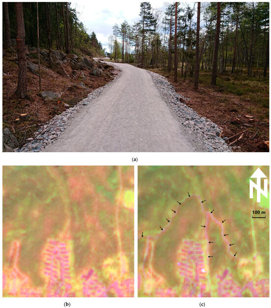
Figure 1.
New road at 59.96901667 degrees north, 10.74830556 degrees east in Oslo, Norway. (a) Photo of the new road. (b) 1 km by 1 km part of the Sentinel-2 image from 2 June 2018, prior to the construction of the road. (c) Sentinel-2 image of the same area from 24 June 2022, after the construction of the new road, with the location of the new road indicated with black arrows.
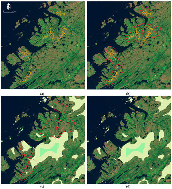
Figure 2.
Steps for updating the map of undisturbed nature. (a) New roads (orange) in the new windmill parks in the Åfjord municipality, Trøndelag County, Norway, superimposed on a 25 km by 25 km part of the Sentinel-2 tile T32WNS of 30 July 2019. (b) 1 km buffer zones around the new roads (red), (c) areas of undisturbed nature (white and mint green) and buffer zones for new roads (red). (d) Remaining areas of undisturbed nature after subtracting the overlaps with the buffer zones.
When trying to improve the prediction performance, one has several options. Firstly, one should analyze if the selected method solves the correct type of problem, or if one could use a method that solves a simpler problem. In image detection, there are four major types of problem (Figure 3):

Figure 3.
Different types of image detection tasks. (a) Image classification. (b) Object detection, with red bounding boxes indicating roads and yellow bounding boxes indicating houses. (c) Semantic segmentation, with roads indicated in green and houses indicated in purple. (d) Instance segmentation, with each object instance in a different colour.
- Image classification: list which objects are in the image [14];
- Object detection: find the bounding box and object type of all the objects in the image [15];
- Semantic segmentation: find the pixels for each type of object in the image [10];
- Instance segmentation: find the pixels for each individual object in the image [16].
U-Net [10] (Figure 4) is a method for semantic segmentation, and seemed to be the correct choice since we could then use the prediction results to produce buffer zones. Image classification, on the other hand, is not suitable for producing buffer zones. However, one could imagine that object detection could be used, via training it on short road segments with different rotations, and possibly also including curved roads and road intersections with different rotations. Although possible, this alternative looks like something one would do if U-Net (or other methods for semantic segmentation) was not available. The last alternative, instance segmentation, could be used, since it would produce results that could be used to create buffer zones. However, instance segmentation is slightly more difficult than semantic segmentation, with no obvious added value for road detection.
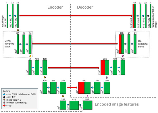
Figure 4.
U-Net architecture used in this study. Input images of size 512 by 512 pixels (upper left) are down-sampled four times to produce encoded image features on a 32 by 32 pixels grid (bottom right), which are then up-sampled four times to produce an output segmentation image of the same resolution as the input image. Skip connections (red horizontal arrows) are used to preserve the image detail during the up-sampling.
Secondly, one could analyze if the selected U-Net has an appropriate input image size and resolution. If the objects are large relative to the image size, one could consider resampling the images to a coarser resolution, provided the objects are still clearly visible with sufficient detail in the coarser resolution. Alternatively, one could use a deeper U-Net; by adding an extra down-sampling block in the encoder and an extra up-sampling block in the decoder, one could double the width and the height of the input images, thus increasing the spatial context for prediction. However, this requires a larger amount of training data. Conversely, if one has too little training data for the U-Net that takes input images of 512 by 512 pixels, one may reduce the input image size, the output image size, and the internal image sizes in the U-Net architecture.
Thirdly, one could analyze if one needs to train on more data. The crucial question to ask is if the training data captures all the expected variation in the input data; if not, how can one obtain more training data? If the amount of training data are limited, one may perform data augmentation on the existing training data, e.g., random cropping, rotation, flipping, scaling, adding noise, and variations in contrast, intensity, color saturation, and the presence or absence of shadows. In addition, one may use a network that has been pre-trained on a large image database such as ImageNet, and then fine-tune the pre-trained net on one’s own data. One limitation is that the pre-training data and one’s own data must have the same number of bands. Since the pre-training is usually carried out on ordinary RGB images, this precludes fine-tuning on images with more than three bands, such as Sentinel-2 images with four spectral bands in 10 m resolution and another six bands in 20 m resolution, the latter six often being resampled to 10 m resolution. Alternatively, one may perform pre-training on a more similar dataset, with the correct number of bands, provided one has access to some ground truth labels for the data.
Fourthly, one could consider some of the new developments in deep neural networks. One such is vision transformers [17]. One could train a foundation model on all available Sentinel-2 data by, e.g., using a masked autoencoder. The training data contains random masked patches, and the autoencoder is trained to reproduce the missing parts. The idea is that the foundation model has learned how Sentinel-2 images look. One can then train a head, a small subnetwork that is inserted after the encoder part of the vision transformer, on the labeled training data.
Lastly, there is the possibility of using a time series of data instead of a single image. To perform change detection, one may use one image acquired before a possible change and one after. One could produce a difference image and train a classifier to detect the relevant changes. However, since there are usually many differences between the two images not related to relevant land use changes, this approach usually leads to many false positives. A better approach is to perform image prediction on both of the images separately and compare the prediction results. However, this approach in effect doubles the prediction error rates, since mistakes may be made both in the prediction of the ‘before’ image and in the prediction of the ‘after’ image. So, the preferred approach is to make predictions on the ‘after’ image and compare them to the existing map of the ‘before’ situation. However, we saw that this approach produced many false negatives, as many new roads were missed. Thus, we wanted to investigate if the accumulated predictions on all the new images acquired after the date of the ‘before’ situation map could reduce the number of false negatives. The underlying hypothesis is that the contrast between a new road and the surrounding landscape varies throughout the year due to seasonal variations in vegetation abundance and, possibly to a lesser degree, illumination differences due to seasonal solar elevation differences, and possibly also between years, as a new road may be gradually less visible as tree canopies grow to eventually fill the gap created by a new road (Figure 5).
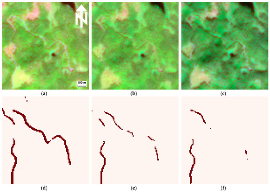
Figure 5.
U-Net prediction results from individual images for a new road at 10.12739722 degrees east, 60.29546667 degrees north, near Elgtjern and Sibekkliveien, Ringerike municipality, Buskerud County. Top row: false-color Sentinel-2 images from (a) 27 July 2018, (b) 31 July 2020, and (c) 22 September 2021, with bands 11, 8, and 3 displayed as red, green, and blue, respectively. Bottom row: predicted roads for (d) 27 July 2018 image, (e) 31 July 2020 image, and (f) 22 September 2021 image.
By using U-Net on all available summer images with less than 10% cloud cover and from a five-year period, the detection rate increased from 26% to 98% compared to using only one cloud-free acquisition. Post-processing steps reduced the false positive rate to 46%. However, as the false positive rate was still substantial, manual verification of the predicted new roads was needed. The false negative rate was low, except in areas without vegetation.
2. Materials and Methods
2.1. Remote Sensing Data
Multispectral optical satellite data from Sentinel-2 processing level 1C, were downloaded for all of Norway for the months of June–September and the years 2018–2022. Images with more than 10% cloud cover were not downloaded. Sentinel-2 captures images of the Earth’s surface in 10 m, 20 m, and 60 m resolution (Table 1). The images are delivered in 100 km by 100 km tiles projected to the nearest UTM zone. To cover all of Norway, 65 image tiles are needed, and they are in the UTM zones 32N, 33N, 34N, and 35N (Figure 5).

Table 1.
Sentinel-2 spectral bands.
Sentinel-2 data can be freely downloaded from https://dataspace.copernicus.eu/ (accessed on 22 October 2024).
Digital terrain model (DTM) data for all of Norway was downloaded from https://hoydedata.no (accessed on 22 October 2024) in a 10 m ground sampling distance. This dataset is based on airborne laser scanning data with 2–10 emitted laser pulses per square meter. The data are available in UTM zones 32N, 33N, and 35N. DTM data for UTM zone 34N were obtained by re-projecting the UTM zone 33N data. The purpose of including DTM data were to remove predicted roads that were too steep. To do this, the terrain gradient was estimated from the DTM using Sobel’s edge detectors (Figure 6).
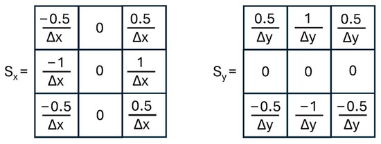
Figure 6.
Sobel’s edge detectors.
The gradient in the east direction, Gx, is obtained by convolving the DTM image with the vertical Sobel edge detector Sx, while the gradient in the north direction, Gy, is the result of convolving the DTM with the horizontal Sobel edge detector, Sy. The constants Δx = Δy = 10 m are the grid cell distances in the east and north directions, respectively, of the DTM.
2.2. Vector Data
Vector data for all the existing roads in Norway were made available to us as ESRI shape files. This included motorways, highways, local roads, and forest roads. Unfortunately, we are not allowed to share this vector data.
2.3. U-Net Deep Neural Network
The U-Net was originally proposed for the semantic segmentation of single-band medical images [10] but can easily be modified to accept input images with several bands. As input, we used 11 bands in 10 m resolution: the four Sentinel-2 bands in 10 m resolution, the six Sentinel-2 bands in 20 m resolution resampled to 10 m resolution, and a scaled version of the gradient magnitude, also in 10 m resolution. The 60 m resolution bands were not used. The gradient of the DTM is a two-band image, with bands and denoting the change in altitude by moving 1 m in the east and north directions, respectively, and were estimated by convolving the DTM with the Sobel edge detectors (see above). The gradient magnitude is the length of the gradient vector . To use the gradient as an extra band in U-Net, the gradient magnitude was scaled to roughly the same value range as the spectral bands, by using . The purpose of including the gradient information as input to U-Net was to allow it to learn terrain types that were unlikely to have new roads constructed.
The U-Net consists of an encoder part and a decoder part (Figure 4). The purpose of the encoder is to extract features that can be used to predict the presence or absence of objects in an image. The purpose of the decoder is to accurately predict the locations of those objects. As an aid in this task, skip connections are made from different image resolutions in the encoder part to similar resolutions in the decoder part. This results in a prediction image of the same resolution as the input image.
A problem with the original U-Net architecture [10] is that each 3 × 3 convolution layer shrinks the image size by one pixel along each of the four image edges, e.g., a 512 × 512 pixel image becomes 510 × 510 after one 3 × 3 convolution. Thus, after all the convolutions of the U-Net, a 572 × 572 input image results in a 388 × 388 output segmentation map. To overcome this, we have modified the convolutions to use the partial convolution method of Liu et al. [18]. Thus, the image sizes are preserved through convolutions, with only minor edge effects.
However, predictions near the image edges may still be unreliable. Therefore, predictions must be made on the overlapping images, with the prediction results clipped along the centers of the overlaps. We used images of 512 by 512 pixels in size as input to U-Net, with 50 pixels overlap with neighboring images to eliminate any remaining edge effects.
2.4. Training of U-Net
The ground truth vector data of the existing roads was converted to raster data matching each 100 km by 100 km Sentinel-2 tile. A buffer of ‘ignore’ pixels were added to each road to remove pixels that could otherwise confuse the learning process.
Of the 65 Sentinel-2 tiles covering Norway (Figure 7), 24 were used for training of the internal weights in the U-Net, while four were used for validation, i.e., selecting which of the several sets of weights to keep, and thus also part of the training procedure. 11 tiles were reserved for testing; of these, two were used in the quantitative evaluation, while the remaining nine were reserved for qualitative evaluation and possible future inclusion in quantitative evaluation. 26 tiles were discarded from the study; of these, 15 were partially outside Norway, so that ground truth data were partially missing; four had large overlaps with other tiles, and the remaining nine covered only smaller parts of the land and large parts of the ocean.
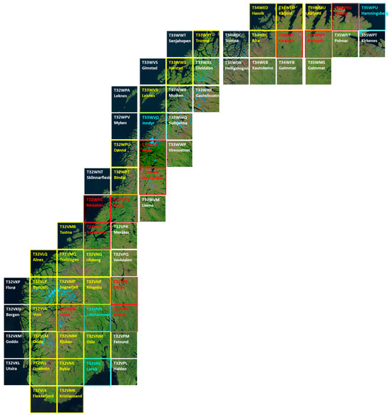
Figure 7.
The 65 Sentinel-2 tiles covering Norway, of which 24 were used for training (yellow), four were used for validation (also part of training; cyan), and 11 were reserved for testing (red).
Training parameters are listed in Table 2.

Table 2.
Parameters used in training of U-Net.
2.5. Automated Prediction Pipeline
An automated processing chain was coded in Python and run as a pilot service at the Norwegian Computing Center. The following steps were run:
- (1)
- Download Sentinel-2 data in level 1C form, not yet downloaded, for the Sentinel-2 tiles covering all of Norway (Figure 7), from the months of June–September and the years of 2018–2022, and with cloud cover less than 10%;
- (2)
- Resample 20 m resolution bands to 10 m resolution using cubic interpolation;
- (3)
- Add the scaled gradient magnitude, as an extra band. Thus, 11 bands in total are used as input to U-Net;
- (4)
- Create a false color image, using bands 11, 8, and 3 as red, green, and blue, respectively. This image may be used for the visual inspection of prediction results;
- (5)
- Predict roads using the trained U-Net;
- (6)
- Remove spurious road predictions within five pixels from the image edges;
- (7)
- Accumulate the prediction results for a tile. For each pixel, the number of times a road was predicted is kept (Figure 8a);
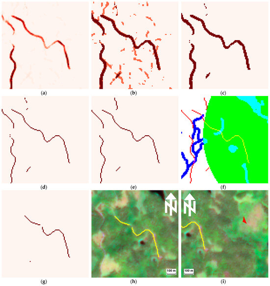 Figure 8. Results of post-processing steps after U-Net prediction, for the same area as in Figure 5. (a) Merged prediction results after step (7). (b) Manipulated version of (a), with pixels predicted as road only once in pale red, and pixels predicted as road twice or more in dark red. (c) Thresholded version of (a) after step (8), keeping pixels predicted as road at least two times. (d) Thinned road predictions, after step (9). (e) Short gaps are closed, after step (10). (f) Masking of predicted roads. Green: buffer zone for areas of undisturbed nature; roads overlapping this zone will reduce the area of undisturbed nature. Blue and cyan: water mask. (g) Masked road predictions, after step (11). (h) Yellow: predicted new roads that will reduce the area of undisturbed nature, after step (12), superimposed on false-color Sentinel-2 image from 24 June 2022. (i) Red: predicted reduction in undisturbed nature, after step (13).
 - (8)
- Threshold the accumulated predictions so that only pixels with at least two road predictions are kept (Figure 8c);
- (9)
- Skeletonize, i.e., apply thinning, so that all the predicted roads are one pixel wide (Figure 8d);
- (10)
- Close short gaps (Figure 8e), using three steps:
- Morphological dilation with a 5 by 5 disk kernel;
- Morphological closing with a 3 by 3 disk kernel;
- Skeletonize;
- (11)
- Mask the thinned road predictions using four steps (Figure 8f,g):
- Remove road predictions that do not overlap a 300 m buffer zone around existing roads. Although many false positives were removed by this step, some occasional fragmented road segments could also be removed;
- Remove predicted roads that are steeper than 30% on average. This criterion was the main reason why one-pixel-wide predicted roads were needed. The DTM was used to compute the steepness of each road, by accumulating the unsigned elevation differences between the neighboring pixels along the road and dividing by the road length;
- Mask the predicted road pixels covered by water. The water mask was created from vector data, using a buffer width of 15 m. The vector data contained ocean, lakes, and rivers;
- Use buffer analysis to discard roads that are not reducing the area of undisturbed nature. A 950 m buffer around all the areas of undisturbed nature was used, since a 1000 m buffer would include many existing roads;
- (12)
- Convert predicted new roads from raster to vector (Figure 8h);
- (13)
- For each predicted new road, create a 1000 m buffer zone and find the intersections with the current polygons of undisturbed nature (Figure 8i). These intersections are the predicted reductions in undisturbed nature;
- (14)
- For each Sentinel-2 tile, upload predicted new roads, predicted reductions in undisturbed nature, and corresponding false-color images to an FTP site for download by the Norwegian Environment Agency.
Steps (1)–(6) were run on each Sentinel-2 file (Figure 9), while the input to step (7) was all single-date road predictions for a given Sentinel-2 tile (Figure 10).
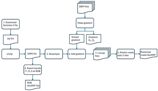
Figure 9.
Data flow diagram for the processing chain for a single Sentinel-2 file, resulting in two GeoTIFF raster files: (1) a false-color RGB image and (2) a binary image with predicted roads.
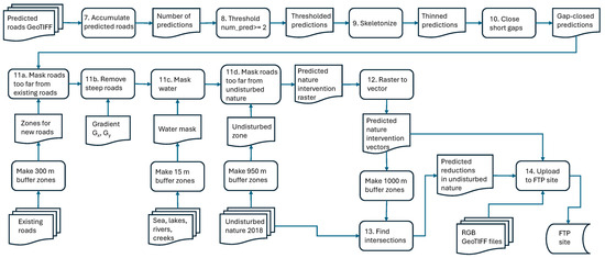
Figure 10.
Data flow diagram for the processing chain for merging all single-date road predictions for the same Sentinel-2 tile and applying several post-processing steps to produce two vector files: (1) predicted nature interventions that will reduce the area of undisturbed nature and (2) predicted reductions in undisturbed nature. The last step is to upload the two vector files plus false-color RGB images of all the contributing Sentinel-2 images to an FTP site.
3. Results
When running the automated processing chain on all Sentinel-2 acquisitions of tile T32VNR with less than 10% cloud cover for the months of June–September and the years of 2018–2022, the method was able to correctly predict 61 new roads (98%), while one new road was missing (Table 3). This assessment was based on visual inspection, since ground truth data were missing. However, for some of the correctly predicted new roads, parts of the new road were missing. The total number of predicted new roads was 114, of which 61 were correct predictions (54%) and 53 were false positives (46%). The importance of merging the predictions on multiple dates in multiple years was illustrated by running U-Net on one cloud-free acquisition only, which resulted in only 16 (26%) of the true new roads being correctly identified (Table 3).

Table 3.
Prediction results on test tile T32VNR.
Please note that the new roads that would not reduce the area of undisturbed nature were masked from the prediction results (step (11)d in Section 2.5). Please also note that the number of missing predictions may be too low for two reasons. Firstly, inspecting an entire 100 km × 100 km tile was considered too time consuming. Secondly, as noted above, a new road may be difficult to see in a single image, even if it is cloud free, so images from several acquisition dates would have to be inspected.
New gravel roads to private cabins were correctly predicted at many locations, e.g., at Hovollkneppet in the Orkland municipality (Figure 11), and in Møssingdalen in the Levanger municipality (Figure 12), both in Trøndelag County. For both these locations, recent aerial images were used for their verification. New forest roads used for the logging of timber were correctly predicted at some locations, e.g., at Lian in the Melhus municipality (Figure 13). There were also several false predictions of new roads. At Bjørklund in the Levanger municipality, Trøndelag County (Figure 14), a temporary vehicle track from the logging of timber was falsely predicted as a new road.
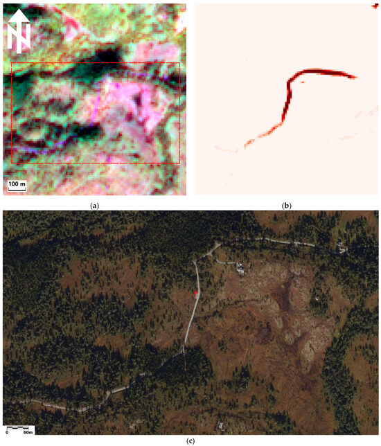
Figure 11.
Predicted new road at 63.04839468 degrees north, 9.87150774 degrees east, near Hovollkneppet in the Orkland municipality, Trøndelag County. (a) Sentinel-2 image from 28 August 2021 in false colors, with bands 11 (shortwave infrared, 1613 nm), 8 (near-infrared, 833 nm), and 3 (green, 560 nm), displayed as red, green, and blue, respectively. Image portion covers 1080 m × 1130 m of the terrain. (b) Accumulated U-Net predictions, with dark colors indicating the predictions at several acquisition dates. (c) Air photo from 28 August 2021, with a red needle indicating the coordinate position. The extent of (c) is indicated with a red rectangle in (a). All the aerial images in the manuscript are from https://norgeibilder.no/ (accessed on 22 October 2024) © Statens kartverk/The Norwegian Mapping Authority.
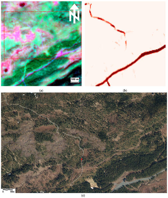
Figure 12.
Predicted new road at 63.58641394 north, 11.08816960 east, near Møssingdalen in the Levanger municipality, Trøndelag County. (a) Sentinel-2 image from 5 July 2018 in false colors. (b) Accumulated predictions, with dark colors indicating predictions at several acquisition dates. (c) Air photo from 17 May 2019, with a red needle indicating the coordinate position. The extent of (c) is indicated with a red rectangle in (a).
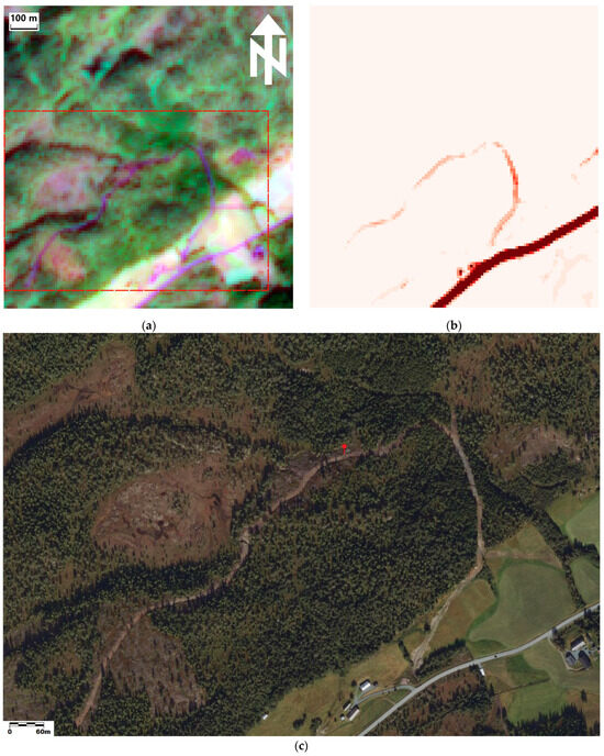
Figure 13.
Predicted new road at 63.10029200 north, 10.11278774 east, near Lian in the Melhus municipality, Trøndelag County. (a) Sentinel-2 image from 28 August 2021 in false colors. (b) Accumulated predictions, with dark colors indicating predictions at several acquisition dates. (c) Air photo from 28 August 2021, with a red needle indicating the coordinate position. The extent of (c) is indicated with a red rectangle in (a).
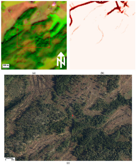
Figure 14.
Predicted new road at 63.66659885 north, 11.06880100 east, near Bjørklund in the Levanger municipality, Trøndelag County. (a) Sentinel-2 image from 28 August 2021 in false colors. (b) Accumulated predictions, with dark colors indicating the predictions at several acquisition dates. (c) Air photo from 17 May 2019, with a red needle indicating the coordinate position. The extent of (c) is indicated with a red rectangle in (a).
In the other test tiles, we looked for interesting cases that could indicate weaknesses of the proposed method. In tile T33WVP, a new road, which was leading to an area with new windmills, was detected (Figure 15) when there was a high spectral contrast between the gravel road and the surrounding terrain due to vegetation cover. However, in areas at higher elevation, with no vegetation cover, the new roads were not predicted, possibly due to low contrast between the gravel road and bare rock surfaces (Figure 16).
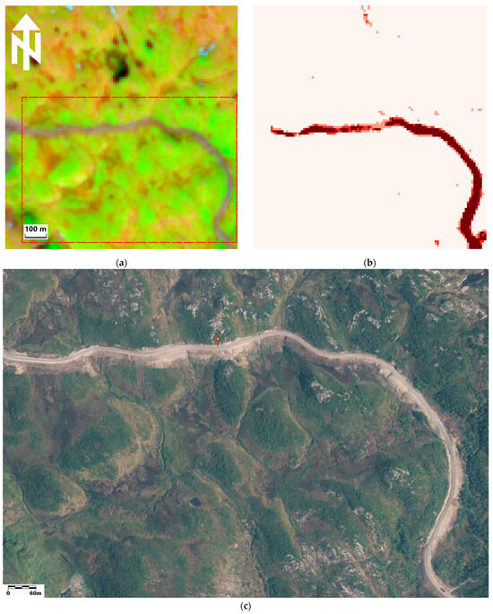
Figure 15.
Predicted new road at 65.83403551 degrees north, 13.09592566 degrees east, at Middagseidklumpen in the Vefsn municipality, Nordland County. (a) Sentinel-2 image from 28 August 2021 in false colors. (b) Accumulated predictions, with dark colors indicating the predictions at several acquisition dates. (c) Air photo from 28 August 2021, with red a needle indicating the coordinate position. The extent of (c) is indicated with a red rectangle in (a).
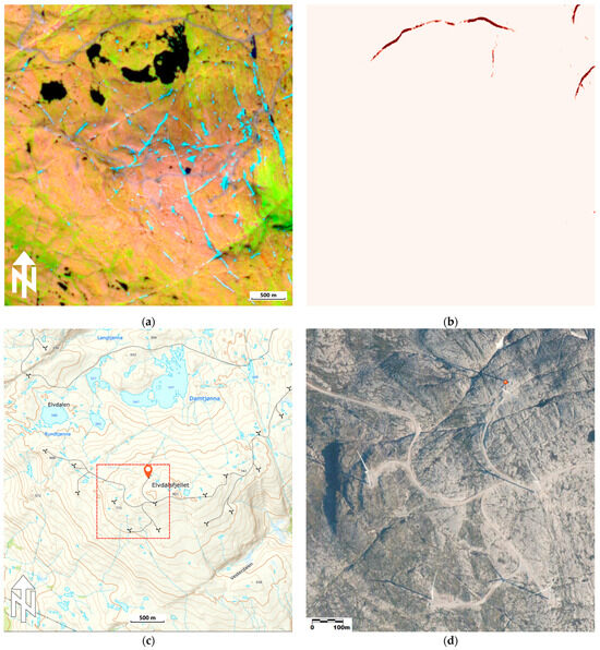
Figure 16.
Missing predictions of new roads at 65.80641667 degrees north, 13.03387222 degrees east, at Elvdalsfjellet in the Vefsn municipality, Nordland County. (a) Sentinel-2 image from 28 August 2021 in false colors; the image portion covers 4320 m × 4520 m of terrain. (b) Accumulated predictions, with dark colors indicating predictions at several acquisition dates. (c) Official map, from https://www.norgeskart.no/ (accessed on 22 October 2024), © Statens kartverk/The Norwegian Mapping Authority. (d) Air photo from 28 August 2021, with a red needle indicating the coordinate position. The area covered by (d) is indicated with a red square in (c).
Although the purpose was to detect new roads not present in the ground truth data, we also wanted to perform a quantitative test of the U-Net’s performance on existing roads in the test data. For this purpose, we compared the prediction results obtained from step 5 in Section 2.5 on single cloud-free acquisitions of tiles T32VMN and T32VNR (Table 4). These tiles, covering the areas around Geilo and Trondheim, respectively, were not seen during training. Three versions of the ground truth data were used. The best prediction performance was achieved when ignore buffers around all the roads were used in both training and testing (Table 4), with an average true positive rate of 57%. When the ignore buffers were not included but replaced with ‘background’ in the ground truth data, the true positive rate dropped to 41% on average.

Table 4.
Pixel-wise prediction results on cloud-free test data.
The road vector data also contained vehicle tracks. If these were included in the ground truth data for both training and testing, but ignore buffers were not included, the true positive rate dropped further to 29% on average (Table 4).
Two other trends could be observed (Table 4). Firstly, the true positive rate varied between image acquisition dates, e.g., from 48% to 68% for tile T32VNR for roads with ignore buffers. This indicates that the contrast between the roads and the background varies over time. Secondly, the false positive rate is three times higher on average when ignore buffers are used versus skipped. However, a false positive rate of 18% is manageable, in the sense that all the predictions must be checked manually whether the false positive rate is 6% or 18%.
4. Discussion
The proposed method, based on U-Net and subsequent post-processing steps, seemed to be able to predict almost all new nature interventions in the form of new roads in areas with vegetation cover. By using all the available summer images with less than 10% cloud cover and from the last five years, the detection rate increased from 26% to 98% for one of the test tiles, compared to using only one cloud-free acquisition. The post-processing steps reduced the false positive rate to 46%.
In some cases, parts of the new roads were missing. However, this could to some extent be ignored, as we constructed 1 km buffer zones around new roads to analyze if they would reduce the current area of undisturbed nature or not. On the other hand, parts of a long new road with several gaps could be lost due to the post-processing step that removed predicted new roads that were too far from existing roads. A possible workaround could be to iteratively add new road segments to the existing roads, thus jumping across gaps one after another.
Also, in areas without vegetation cover, new roads were not predicted. Usually, one would avoid building new roads in such areas, since the lack of vegetation is usually caused by long winters with snow cover from early autumn until late spring, which in turn would imply high road maintenance costs. One important exception to such considerations is the recent erection of windmills in some such areas. However, the Norwegian Environment Agency has recently made an agreement with the Norwegian Mapping Authority (in Norwegian: Statens kartverk) to obtain new windmill positions and associated new roads inserted into the national mapping much more frequently than the regular map update cycle.
In an automatic prediction system, it would be a problem if parts of a new road were missing, since the resulting reduction in undisturbed nature could also be too small as a consequence. However, since the false positive rate was quite high (46%), all the predicted new roads had to be manually checked, and missing parts would usually be spotted as part of that, but at the extra cost of editing the prediction results.
The time needed for the manual verification of the predicted new roads varied from case to case. If a new air photo was available, the verification of a single predicted new road could be performed in 5–15 min. If no new air photo was available, then the manual inspection of the satellite image was not always conclusive, and other sources were checked, e.g., if there was an application for constructing a new road. The last resort could be to conduct a field visit, which usually requires one full working day, which was usually not feasible.
In order to train U-Net more specifically for forest road detection, the training procedure could be split into two parts. First, one could use all the training data to pre-train U-Net for general road detection. Then, one could fine-tune U-Net for forest road detection by including only the parts of the training data that contain forest roads.
In order to better capture new roads that were fragmented in the prediction result, we could use super-resolution. Ayala et al. [9] used bicubic interpolation to increase the resolution from 10 m to 2.5 m, then used U-Net to predict roads at 2.5 m resolution. In this way, they achieved less fragmented roads compared to using U-Net on 10 m resolution data, improving the intersection over union score from 37% to 69%. Sarmad et al. [19] used diffusion models to achieve 2.5 m super-resolution in Sentinel-2 images, without the need for paired high-resolution training data.
There is some potential in training U-Net in a more focused way. Since the new roads in areas with no vegetation are possible to see in the satellite images, it should also be possible to train U-Net to detect them. One problem could be that we have only used one common class for all roads. Thus, we could either try to use a separate road class for roads in areas with no vegetation, and possibly separate road classes in some other cases too. Alternatively, we could train a separate U-Net classifier for roads in areas without vegetation.
An alternative method for the detection of windmills could be to use Sentinel-1 radar satellite images. Initial experiments indicated that most new windmills were visible in difference images, with one Sentinel-1 acquisition before the windmills were built and another Sentinel-1 acquisition after. However, there were also numerous false positives in the difference images. Thus, this alternative approach was not further pursued.
While our current method effectively utilizes temporal data by aggregating predictions from multiple dates, future research could explore the integration of recurrent neural networks, such as long short-term memory (LSTM), to further leverage the temporal dynamics of road construction and potentially improve detection accuracy.
As an alternative to using the spectral bands as input to U-Net, it would be possible to use one or more vegetation indices instead of, or in addition to, some or all the spectral bands. Bakkestuen et al. [20] combine 10 spectral indexes and three spectral bands for wetland delineation from Sentinel-2 images using U-Net. However, while explicit spectral indices could be considered as additional input features, the inherent feature extraction capabilities of U-Net may enable it to implicitly capture vegetation characteristics from the existing spectral bands.
Even though U-Net is already nine years old, it still remains a strong and widely used option, often considered a standard approach for segmentation tasks. Its effectiveness and efficiency have been demonstrated in various applications. We have therefore chosen to improve U-Net by adding post-processing steps, and not performing an extensive comparison to other network architectures. Recent models based on vision transformers (ViT) [17] may perform better than U-Net, if the ViT has been trained using self-supervised learning on a vast number of Sentinel-2 images. However, the ViT alone is not sufficient; we also need a decoder that can perform the mapping of roads, which are often barely visible, with high accuracy. A potential decoder architecture for this task is SegViTv2 [21], which has proven to be effective compared to other decoder architectures. However, due to the challenge of segmenting roads, it may also be necessary to investigate other architectures like dense prediction transformers [22] or FeatUp [23], in order to improve the resolution.
5. Conclusions
The present study shows that the automated detection of new roads in Sentinel-2 images is possible, with a high true positive rate. However, as the false positive rate is nearly 50%, manual verification of the predicted new roads is needed. The false negative rate was low, except in areas without vegetation.
The low false negative rate was achieved by merging predictions from all the June–September images from five years and with less than 10% cloud cover. Compared to using a single cloud-free image for prediction, the false negative rate was reduced from 74% to 2%. Several post-processing steps were used to reduce the false positive rate from more than 100% to 50%.
Future research should focus on ways to reduce the false positive rate, as this is the main obstacle in reducing the need for the manual verification of the predicted new roads. However, given the spatial resolution of 10 m, it seems difficult to reduce the false positive rate to zero. But super-resolution methods [11,12,19] could be attempted and might also make the manual verification of Sentinel-2 images easier.
Author Contributions
Conceptualization, Ø.D.T. and A.-B.S.; methodology, A.-B.S. and Ø.D.T.; software, Ø.D.T.; validation, Ø.D.T.; formal analysis, Ø.D.T.; investigation, Ø.D.T.; data curation, Ø.D.T.; writing—original draft preparation, Ø.D.T. and A.-B.S.; writing—review and editing, Ø.D.T. and A.-B.S.; visualization, Ø.D.T.; project administration, Ø.D.T. All authors have read and agreed to the published version of the manuscript.
Funding
This research was funded by the Norwegian Space Centre through their Copernicus program.
Data Availability Statement
Sentinel-2 data can be freely downloaded from https://dataspace.copernicus.eu/ (accessed on 22 October 2024; global coverage) and https://colhub.met.no/ (accessed 22 on October 2024; Norway only). Digital terrain model data for Norway can be freely downloaded from https://hoydedata.no (accessed on 22 October 2024). The official map of Norway is available as raster images at https://www.norgeskart.no/ (accessed on 22 October 2024); however, the original vector data are not freely available. Aerial images of Norway are available at https://norgeibilder.no/ (accessed on 22 October 2024).
Acknowledgments
We thank Ragnvald Larsen and Ole T. Nyvoll at the Norwegian Environment Agency for funding acquisition, for providing a challenging research problem, for providing ground truth data for all existing roads in Norway, and for their assistance in the assessment of the methodology and validation of the prediction results. We thank the anonymous reviewers for critical comments, which helped to improve the manuscript.
Conflicts of Interest
The authors declare no conflicts of interest. The funders had no role in the design of this study; in the collection, analyses, or interpretation of the data; in the writing of the manuscript; or in the decision to publish the results; however, there was a requirement for funding that satellite data be used.
References
- Jaeger, J.A. Landscape division, splitting index, and effective mesh size: New measures of landscape fragmentation. Landsc. Ecol. 2000, 15, 115–130. [Google Scholar] [CrossRef]
- Torres, A.; Jaeger, J.A.G.; Alonso, J.C. Assessing large-scale wildlife responses to human infrastructure development. Proc. Natl. Acad. Sci. USA 2016, 113, 8472–8477. [Google Scholar] [CrossRef] [PubMed]
- Sverdrup-Thygeson, A.; Søgaard, G.; Rusch, G.M.; Barton, D.N. Spatial overlap between environmental policy instruments and areas of high conservation value in forest. PLoS ONE 2014, 9, e115001. [Google Scholar] [CrossRef] [PubMed]
- Lehmler, S.; Förster, M.; Frick, A. Modelling green volume using Sentinel-1, -2, PALSAR-2 satellite data and machine learning for urban and semi-urban areas in Germany. Environ. Manag. 2023, 72, 657–670. [Google Scholar] [CrossRef] [PubMed]
- Deche, A.; Assen, M.; Damene, S.; Budds, J.; Kumsa, A. Dynamics and drivers of land use and land cover change in the Upper Awash Basin, Central Rift Valley of Ethiopia. Environ. Manag. 2023, 72, 160–178. [Google Scholar] [CrossRef] [PubMed]
- Demichelis, C.; Oszwald, J.; Mckey, D.; Essono, P.Y.B.; Sounguet, G.P.; Braun, J.J. Socio-ecological approach to a forest-swamp-savannah mosaic landscape using remote sensing and local knowledge: A case study in the Bas-Ogooué Ramsar site, Gabon. Environ. Manag. 2023, 72, 1241–1258. [Google Scholar] [CrossRef] [PubMed]
- Brandão, A.O., Jr.; Souza, C.M., Jr. Mapping unofficial roads with Landsat images: A new tool to improve the monitoring of the Brazilian Amazon rainforest. Int. J. Remote Sens. 2006, 27, 177–189. [Google Scholar] [CrossRef]
- Ahmed, M.W.; Saadi, S.; Ahmed, M. Automated road extraction using reinforced road indices for Sentinel-2 data. Array 2022, 16, 100257. [Google Scholar] [CrossRef]
- Ayala, C.; Aranda, C.; Galar, M. Towards fine-grained road maps extraction using Sentinel-2 imagery. ISPRS Ann. Photogramm. Remote Sens. Spat. Inf. Sci. 2021, V-3-2021, 9–14. [Google Scholar] [CrossRef]
- Ronneberger, O.; Fischer, P.; Brox, T. U-Net: Convolutional networks for biomedical image segmentation. In: Medical Image Computing and Computer-Assisted Intervention–MICCAI 2015. Part III. Lect. Notes Comput. Sci. 2015, 9351, 234–241. [Google Scholar] [CrossRef]
- Sirko, W.; Brempong, E.A.; Marcos, J.T.C.; Korme, A.A.A.; Hassen, M.A.; Sapkota, K.; Shekel, T.; Diack, A.; Nevo, S.; Hickey, J.; et al. High-resolution building and road detection from Sentinel-2. arXiv 2024, arXiv:2310.11622. [Google Scholar] [CrossRef]
- Jia, Y.; Zhang, X.; Xiang, R.; Ge, Y. Super-resolution rural road extraction from Sentinel-2 imagery using a spatial relationship-informed network. Remote Sens. 2023, 15, 4193. [Google Scholar] [CrossRef]
- Trier, Ø.D.; Salberg, A.B.; Larsen, R.; Nyvoll, O.T. Detection of forest roads in Sentinel-2 images using U-Net. In Proceedings of the Northern Lights Deep Learning Workshop, Virtual, 10–12 January 2022; Volume 3. 8p. [Google Scholar] [CrossRef]
- Krizhevsky, A.; Sutskever, I.; Hinton, G.E. ImageNet classification with deep convolutional neural networks. Commun. ACM 2017, 60, 84–90. [Google Scholar] [CrossRef]
- Ren, S.; He, K.; Girshick, R.; Sun, J. Faster R-CNN: Towards real-time object detection with region proposal networks. IEEE Trans. Pattern Anal. Mach. Intell. 2017, 39, 1137–1149. [Google Scholar] [CrossRef] [PubMed]
- He, K.; Gkioxari, G.; Dollar, P.; Girshick, R. Mask R-CNN. In Proceedings of the IEEE International Conference on Computer Vision (ICCV), Venice, Italy, 22–29 October 2017; pp. 2961–2969. [Google Scholar] [CrossRef]
- Zhang, B.; Tian, Z.; Tang, Q.; Chu, X.; Wei, X.; Shen, C.; Liu, Y. SegViT: Semantic segmentation with plain vision transformers. In Proceedings of the 36th Conference Neural Information Processing Systems, New Orleans, LA, USA, 28 November–9 December 2022; pp. 4971–4982. [Google Scholar] [CrossRef]
- Liu, G.; Reda, F.A.; Shih, K.J.; Wang, T.-C.; Tao, A.; Catanzaro, B. Image inpainting for irregular holes using partial convolutions. In: The 15th European Conference on Computer Vision (ECCV), 8–14 September 2018, Munich, Germany. Lect. Notes Comput. Sci. 2018, 11215, 89–105. [Google Scholar] [CrossRef]
- Sarmad, M.; Kampffmeyer, M.; Salberg, A.-B. Diffusion models with cross-modal data for super-resolution of Sentinel-2 to 2.5 meter resolution. In Proceedings of the 2024 IEEE International Geoscience and Remote Sensing Symposium, Athens, Greece, 7–12 July 2024; pp. 1103–1107. [Google Scholar] [CrossRef]
- Bakkestuen, V.; Venter, Z.; Ganerød, A.J.; Framstad, E. Delineation of wetland areas in South Norway from Sentinel-2 imagery and lidar using TensorFlow, U-Net, and Google Earth Engine. Remote Sens. 2023, 15, 1203. [Google Scholar] [CrossRef]
- Zhang, B.; Liu, L.; Phan, M.H.; Tian, Z.; Shen, C.; Liu, Y. SegViT v2: Exploring efficient and continual semantic segmentation with plain vision transformers. Int. J. Comput. Vis. 2024, 132, 1126–1147. [Google Scholar] [CrossRef]
- Ranftl, R.; Bochkovskiy, A.; Koltun, V. Vision transformers for dense prediction. arXiv 2021, arXiv:2103.13413. [Google Scholar] [CrossRef]
- Fu, S.; Hamilton, M.; Brandt, L.E.; Feldmann, A.; Zhang, Z.; Freeman, W.T. FeatUp: A model-agnostic framework for features at any resolution. arXiv 2024, arXiv:2403.10516. [Google Scholar] [CrossRef]
Disclaimer/Publisher’s Note: The statements, opinions and data contained in all publications are solely those of the individual author(s) and contributor(s) and not of MDPI and/or the editor(s). MDPI and/or the editor(s) disclaim responsibility for any injury to people or property resulting from any ideas, methods, instructions or products referred to in the content. |
© 2024 by the authors. Licensee MDPI, Basel, Switzerland. This article is an open access article distributed under the terms and conditions of the Creative Commons Attribution (CC BY) license (https://creativecommons.org/licenses/by/4.0/).