Three-Dimensional Reconstruction of Retaining Structure Defects from Crosshole Ground Penetrating Radar Data Using a Generative Adversarial Network

Abstract

Crosshole ground penetrating radar (GPR) is an efficient method for ensuring the quality of retaining structures without the need for excavation. However, interpreting crosshole GPR data is time-consuming and prone to inaccuracies. To address this challenge, we proposed a novel three-dimensional (3D) reconstruction method based on a generative adversarial network (GAN) to recover 3D permittivity distributions from crosshole GPR images. The established framework, named CGPR2VOX, integrates a fully connected layer, a residual network, and a specialized 3D decoder in the generator to effectively translate crosshole GPR data into 3D permittivity voxels. The discriminator was designed to enhance the generator’s performance by ensuring the physical plausibility and accuracy of the reconstructed models. This adversarial training mechanism enables the network to learn non-linear relationships between crosshole GPR data and subsurface permittivity distributions. CGPR2VOX was trained using a dataset generated through finite-difference time-domain (FDTD) simulations, achieving precision, recall and F1-score of 91.43%, 96.97% and 94.12%, respectively. Model experiments validate that the relative errors of the estimated positions of the defects were 1.67%, 1.65%, and 1.30% in the X-, Y-, and Z-direction, respectively. Meanwhile, the method exhibits noteworthy generalization capabilities under complex conditions, including condition variations, heterogeneous materials and electromagnetic noise, highlighting its reliability and effectiveness for practical quality assurance of retaining structures.

1. Introduction

Due to complex geological conditions and uncertain construction processes, defects such as cracks, sludge accumulation, and voids frequently occur in retaining structures [1,2], weakening the integrity and safety of the structures and resulting in deformation and ground surface settlement [3]. Therefore, accurately locating and identifying defects within these structures is crucial. Crosshole ground penetrating radar (GPR) is particularly suitable for quality inspection of retaining structures due to its high efficiency and sufficient resolution [4]. This method generates high-frequency electromagnetic (EM) waves using a transmitting antenna, which are received by a receiving antenna through boreholes in the retaining structures [5]. By interpreting the measured EM wave data, the dielectric parameter distribution (permittivity and conductivity) of the retaining structure can be inferred based on the differences between defects and intact areas, which helps guide the detection of defects [6,7].

Deriving the dielectric parameters from crosshole GPR measurement involves inverting crosshole GPR data [8]. In the last decades, inversion methods such as ray-based tomography and full-waveform inversion (FWI) have significantly advanced [9]. Ray-based tomography neglects diffraction, scattering, and interference of EM waves, resulting in a limited resolution for the inversion results that is greater than the wavelength [10,11]. In addition, ray-based tomography primarily focuses on two-dimensional (2D) inversion, which fails to fully capture the three-dimensional (3D) characteristics of the detection area [12]. In comparison, FWI methods utilize the entire waveform information and estimate the dielectric parameters by fitting data to crosshole GPR measurements [13,14]. This approach can more accurately handle and describe the 3D characteristics of subsurface structures. However, recovering a 3D dielectric model using FWI methods is extremely expensive in terms of computational resources [15,16]. To accelerate the FWI process, some studies have transformed the 3D reconstruction of crosshole GPR into computations performed on a series of 2D slices, which cannot comprehensively represent the 3D geophysical information of the detection area [17]. Furthermore, the need for an accurate initial model and source wavelet also hinders the application of FWI methods in real-world crosshole GPR data interpretation [8,18].

In recent years, deep learning has become a focal point in the field of computer vision, particularly following the advent of convolutional neural networks (CNNs) [19,20]. Deep learning methods can automatically learn multi-dimensional features from training data and establish the non-linear relationship of cross-domain data [21,22], enabling end-to-end translation from crosshole GPR data to 3D dielectric parameters [23]. However, studies of crosshole GPR data interpretation associated with deep learning methods are currently limited to the reconstruction of 2D dielectric profiles from 2D crosshole GPR images [24,25,26,27]. The 2D deep learning reconstruction frameworks developed in these studies are unable to handle the dimensional expansion computations required for transforming 2D crosshole GPR images into 3D models [28].

Compared with 2D interpretation, 3D interpretation provides a more accurate representation of subsurface structures, which is crucial for improving the quality of crosshole GPR data interpretation [29]. However, the transition from crosshole GPR data to a 3D distribution of permittivity presents a significant challenge due to the complex propagation characteristics of EM waves [30]. The non-linearity of wave propagation and the non-uniqueness of the inversion problem considerably increase the computational difficulty [31]. Additionally, GPR signals are easily affected by external noise, such as environmental EM interference and antenna coupling effects, exacerbating the issue of non-uniqueness in the inversion process and making direct application infeasible [32]. To the best of our knowledge, there are no deep learning-based subsurface reconstruction methods using crosshole GPR data.

In order to facilitate the 3D interpretation of crosshole GPR data for defect detection in retaining structures, we proposed a novel 3D reconstruction method based on a generative adversarial network (GAN) [33] named CGPR2VOX (crosshole GPR to voxel), which maps 2D crosshole GPR profiles directly to 3D permittivity. In this paper, we first introduce the design of the 3D reconstruction method, including the structure of the GAN framework and the preparation of the numerical simulation dataset. In addition, we design a visible experimental model to verify the effectiveness of the network when interpreting real-world crosshole GPR data. Using the experimental data, we also compare the reconstruction results with other interpretation methods to highlight the superiority of our approach. Furthermore, we discuss the generalization ability of CGPRVOX under complex detection conditions involving heterogeneous materials and EM noise. Finally, we summarize the main findings of this study.

2. Methodology

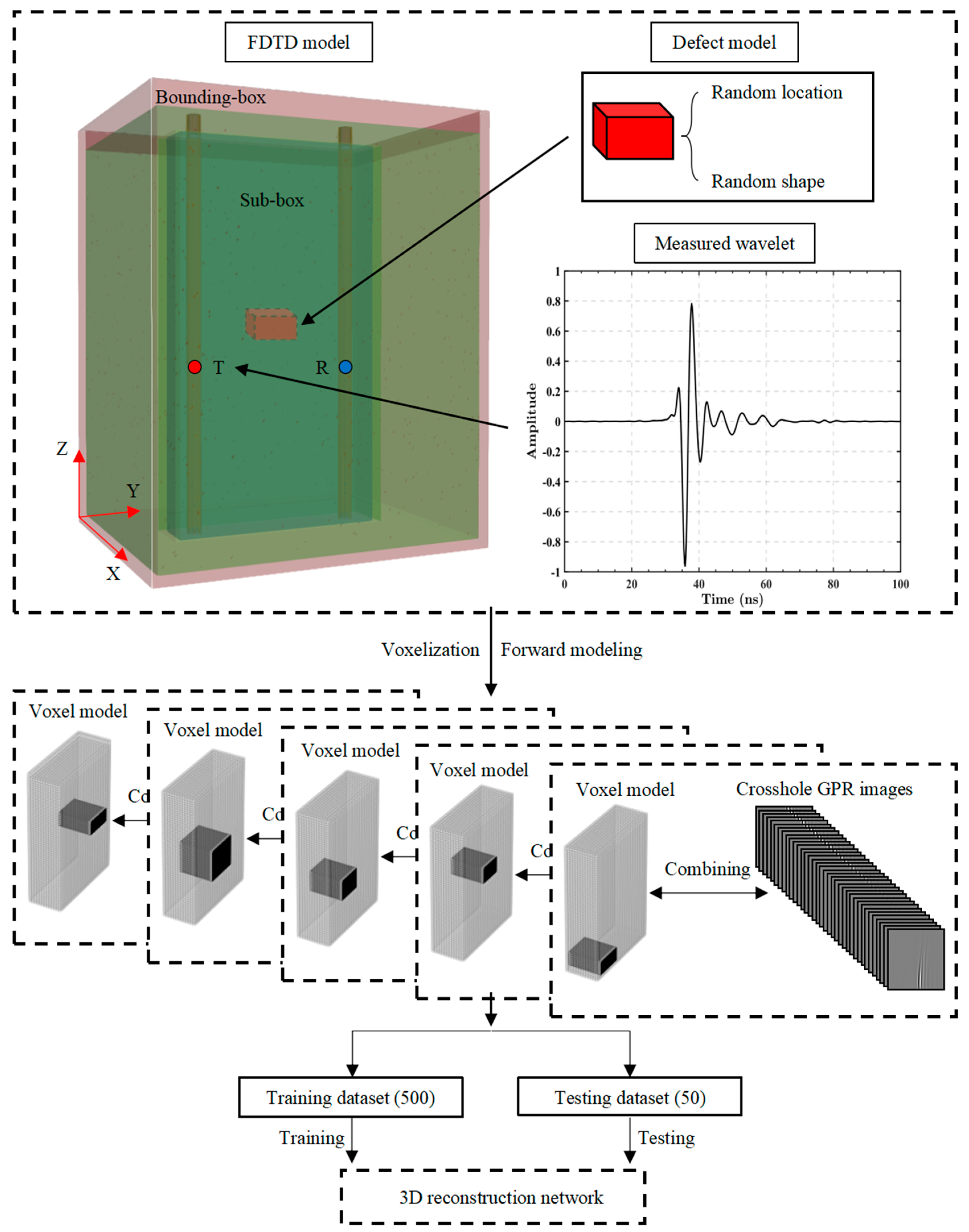
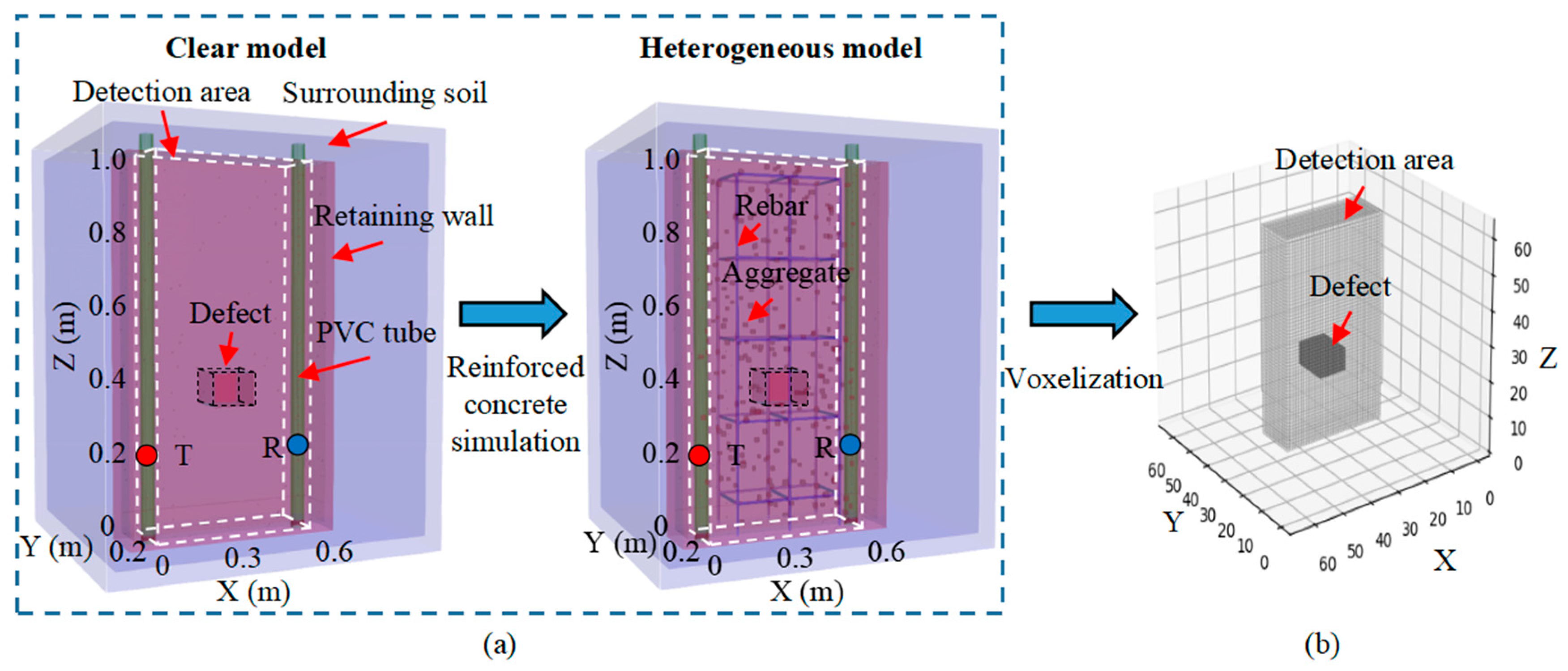
2.1. Crosshole GPR Measurement

Figure 1 illustrates the process of using the crosshole GPR method to inspect the quality of retaining structures. In Figure 1a, two antennas are placed in the boreholes at opposite ends of a retaining structure, serving as transmitting and receiving antennas, respectively. Figure 1b presents the detection process in which the transmitting antenna radiates an omnidirectional EM wave at T1. Then, this wave propagates through the structure and reaches the defect area around time T2. Due to the sudden change in permittivity and conductivity from concrete to defect, most of the EM wave energy penetrates the defect area and forms a direct wave, while the remaining energy reflects off the edge of the defect and forms reflected wave #1. Since the permittivity of the defect is higher than that of the concrete, the direct wave propagates more slowly in the defect than in the concrete. As a result, the direct wave in the concrete generates a diffracted wave behind the defect at time T3. Thereafter, the penetrating wave is formed by the superposition of the direct wave and part of the reflected wave inside the defect, while the other part of the reflected wave is reflected back from the edge, forming reflected wave #2 at time T4. Finally, the energy of the EM wave dissipates completely in this structure at time T5 [34].

Meanwhile, the receiving antenna receives the transmitted EM waves at multiple depths within a time window of T5, as shown in Figure 1c. The first channel of the receiving antenna first receives the direct wave, followed by the penetrating wave, while the ninth channel, which is at the same depth as the defect, receives the diffracted wave first, then the penetrating wave, and finally the reflected wave #2. Similar propagation patterns occur in other channels. After emitting and collecting EM waves at multiple depths, a block of crosshole GPR data is obtained, as depicted in Figure 1d. These data contain information about the dielectric properties of the measured area, and the main task of this work is to reconstruct an accurate 3D permittivity map from the measured crosshole GPR images.

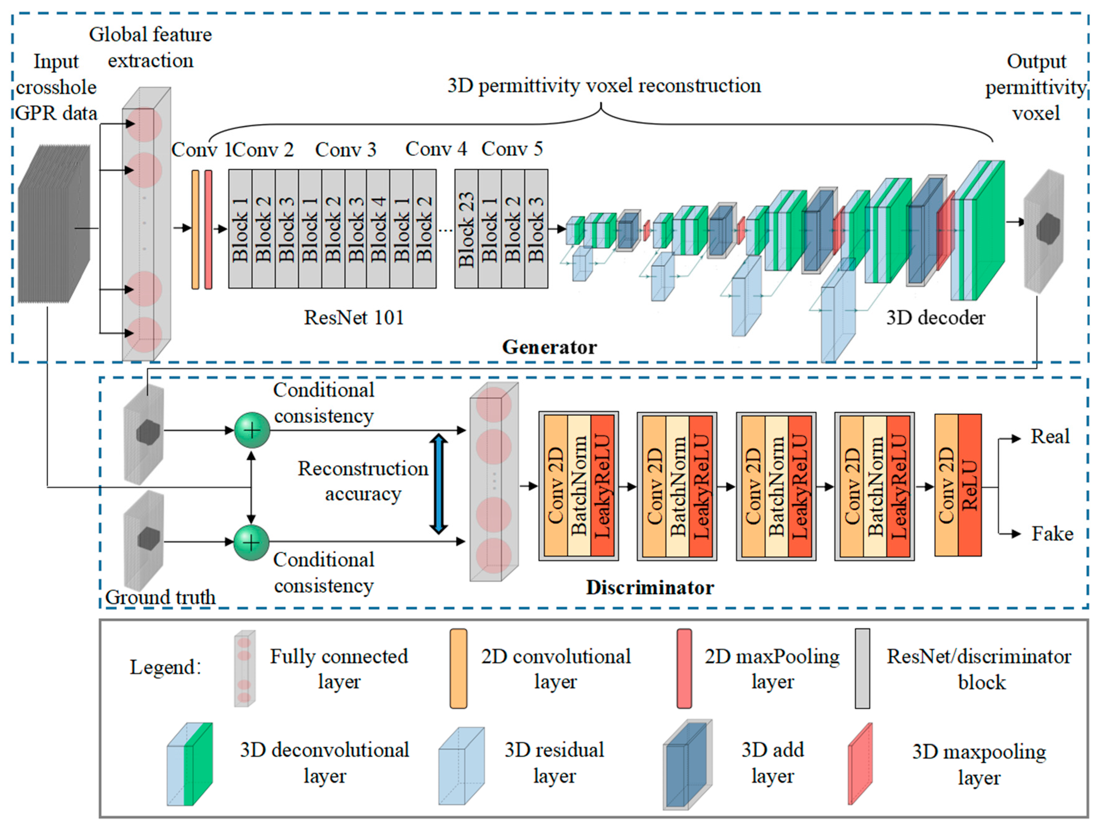
2.2. 3D Reconstruction Network

Reconstructing a 3D permittivity distribution from crosshole GPR data involves solving a fundamental inverse problem, where the objective is to infer the subsurface permittivity model from observed EM wave data. This relationship can be mathematically represented as follows:

$$d=F\left(m\right)+n,$$

(1)

where F represents the forward operator that governs the propagation of EM waves through the subsurface, m is the 3D permittivity distribution to be reconstructed, and n denotes the measurement noise. The challenge lies in finding an appropriate inverse operator F⁻¹ to recover m from d. However, because this inverse problem is both non-linear and ill-posed, finding an analytical solution is nearly impossible.

Herein, we propose a deep learning-based approach using a generative adversarial network (GAN) framework to solve this problem. In the framework, the generator functions as an inversion operator G, which directly estimates the 3D permittivity distribution from the observed data, while the discriminator serves as a regularization method D, evaluating the realism and physical plausibility of the generated models. The overall objective of the inversion problem is to minimize the difference between the predicted and true 3D permittivity distributions while ensuring that the reconstructed models remain physically plausible. This can be formalized as an optimization problem, where the loss function combines a data fidelity term and a regularization term:

$$L(G,D) =L_{\mathrm{d}\mathrm{a}\mathrm{t}\mathrm{a}}(G\left(d\right),m)+\lambda L_{\mathrm{reg}}(G,D)$$

(2)

in this equation, L_data enforces the consistency between the generated model and the observed data, while L_reg ensures the physical plausibility of the reconstructed model. The parameter λ controls the trade-off between data fidelity and regularization. The generator G is responsible for learning the inverse mapping from the data domain to the model domain, approximating the inverse operator F⁻¹. By using a dataset of crosshole GPR data along with corresponding 3D permittivity models, the generator learns to approximate the inverse relationship between d and m. This enables fast, direct inversion, bypassing the iterative techniques typically required by traditional inversion methods.

The discriminator D functions as a regularizer, learning to distinguish between realistic and generated 3D permittivity distributions. It outputs a probability score indicating whether a given model m is real or generated by the generator. This score serves as a feedback mechanism, facilitating iterative improvement of the generator’s performance. The objective function can be expressed as follows [35]:

$$\underset{G}{\min }\underset{D}{\max }\mathrm{V}\left(G,D\right)=E_{x_{\mathrm{p}}~P_{\mathrm{data}}\left(x_{\mathrm{p}}\right)}[\log D(x_{\mathrm{p}}\left)\right]+E_{x_G~P_{\mathrm{data}}\left(x_{\mathrm{p}}\right)}\left[\log \right(1-D(G(x_G\left)\right))],$$

(3)

where the terms $E_{x_{\mathrm{p}}~P_{\mathrm{data}}\left(x_{\mathrm{p}}\right)}[\log D(x_{\mathrm{p}}\left)\right]$ and $E_{x_G~P_{\mathrm{data}}\left(x_{\mathrm{p}}\right)}\left[\log \right(1-D(G(x_G\left)\right))]$ are the mathematical expectations of logarithmic loss when D identifies the real and fake samples, respectively. The discriminator assigns a label of “1” to samples that it recognizes as real and “0” to those it identifies as fake. The objective for D is to maximize the value function V(G, D) by labeling all real samples as “1” and all fake samples generated by G as “0”, i.e., $D\left(x_{\mathrm{p}}\right)$ = 1 and $D\left(G\right(x_G\left)\right)=0$. Conversely, the adversarial G aims to minimize $\mathrm{V}(G,D)$ by generating more realistic samples to obtain the label “1” assigned by the D, that is, $D\left(G\right(x_G\left)\right)=1$. When the performance of D and G are balanced, the objective function can be considered to have reached its optimal value.

In this GAN framework, the generator functions as an effective inversion operator by minimizing the discrepancy between the generated 3D permittivity distribution and the actual EM wave data. Concurrently, the discriminator acts as a robust regularizer, ensuring that the reconstructed models conform to the statistical characteristics of actual permittivity distributions. This adversarial interaction improves the overall performance of the network, facilitating more accurate and physically plausible 3D reconstructions compared to traditional inversion methods. By integrating data fidelity with model regularization, the GAN-based approach overcomes the non-linearity and ill-posedness inherent in the inverse problem, offering a superior solution for 3D permittivity reconstruction from crosshole GPR data.

Based on the analysis above, we designed the CGPR2VOX framework to reconstruct crosshole GPR B-scan images into a 3D permittivity voxel model. Figure 2 depicts the structure of CGPR2VOX, which comprises two stages: global feature extraction and 3D permittivity voxel reconstruction. The global feature extraction stage retrieves global features from crosshole GPR data. Three-dimensional permittivity voxel reconstruction creates a voxel model that represents the 3D permittivity distribution.

2.2.1. Global Feature Extraction

Let x_P represent the real permittivity values of the retaining structure, and x_G denote the EM waves obtained by the crosshole GPR. To establish the non-linear relationship between the two sets of data, we first employed a fully connected (FC) layer with 1024 neurons to extract the global features from x_G. In this FC layer, 74% of the neurons are active, and the remaining 26% remain dormant. Each active neuron connects to all channels of the crosshole GPR data, which is structured as a 64 × 64 × 36 tensor. Specifically, each active neuron is automatically assigned unique weights and biases to each connected channel, and a rectified linear unit (ReLU) activation function is applied. This mechanism enables each active neuron to independently process information from every GPR channel, facilitating the extraction of feature maps with dimensions of 64 × 64 × 1. The diverse weighting ensures that the network captures a wide range of patterns and anomalies in the GPR data, enhancing the model’s ability to learn non-linear relationships. In contrast, each dormant neuron does not connect to any crosshole GPR data but outputs a zero vector with dimensions of 64 × 64 × 1. The inclusion of dormant neurons introduces sparsity in the feature extraction process, ensuring that the network remains robust against noise and irrelevant variations in the input data.

Additionally, the alternating arrangement of active and dormant neurons within the FC layer encourages an implicit feature selection mechanism. By selectively activating a subset of neurons connected to the crosshole GPR data, the network prioritizes channels most relevant to defect reconstruction, extracting global features while ignoring redundant information. This adaptability improves the network’s ability to capture meaningful patterns in the GPR data, thus enhancing the accuracy of the subsequent 3D permittivity reconstruction. By concatenating the output from both active and dormant neurons, a global feature tensor x_FC with dimensions of 64 × 64 × 1024 is formed, establishing the initially global non-linear relationship between the permittivity distribution and crosshole GPR data.

2.2.2. 3D Permittivity Voxel Reconstruction

The global feature x_FC captures the low-order features in the crosshole GPR data, which are insufficient to infer the 3D permittivity distribution. To extract high-order features from x_FC, we utilized the convolutional layers of the ResNet101 V2 network, as shown in Figure 2. This network comprises 100 convolutional layers organized into five groups known as ResNet blocks [36]. As the network depth increases, the convolution blocks progressively enhance the non-linear expressive capability. Consequently, the final ResNet block produces high-order feature maps x_R with dimensions of 2 × 2 × 2048, which can be used to compute the 3D distribution of permittivity.

Next, we designed a 3D decoder to transform the feature maps x_R into permittivity voxels. The 3D decoder uses 14 3D deconvolutional layers to gradually upsample the feature maps and reconstruct the 3D spatial distribution of permittivity values. In the first 12 deconvolutional layers, we inserted a 1 × 1 × 1 deconvolutional layer (kernel size: 13, stride size: 13) after every two 4 × 4 × 4 deconvolutional layers (kernel size: 43, stride size: 23). The last two layers are both 1 × 1 × 1 deconvolutional layers. In addition, to mitigate overfitting and prevent gradient vanishing during decoder training, a residual module and a maxpooling layer are inserted after every three 3D deconvolutional layers. After passing through the 3D decoder, the feature maps x_R are converted to a 3D permittivity voxel with dimensions of 64 × 64 × 64, as depicted on the right side of Figure 2.

2.2.3. Discriminator

We also introduced a discriminator into GPR2VOX to evaluate the authenticity of the generated 3D permittivity models by assessing their conditional consistency with the corresponding crosshole GPR images and comparing their reconstruction accuracy to the ground truth models. Initially, the discriminator processes the combined data pairs (comprising crosshole GPR images and either the generator’s outputs or the ground truth models) through an FC layer to extract global features. Then, these features are fed into a cascade of blocks. Each block consists of a 2D convolutional layer (Conv 2D), a batch normalization layer (Batchnorm), and a LeakyReLU activation function. Finally, a convolutional layer with a ReLU activation function is used to compute the authenticity score.

2.2.4. Loss Function

In this study, we used the mean squared logarithmic error (MSLE) as the loss function of CGPR2VOX [37]:

$$\mathrm{MSLE}\left(P_{\mathrm{pre}},P_{\mathrm{real}}\right)={\displaystyle \frac{1}{m}} {\sum }_{i=1}^m {\left(\log \left(p_{\mathrm{pre},i}+1\right) -\log \left(p_{\mathrm{real},i}+1\right)\right)}^2,$$

(4)

where m is the total number of voxels in the training data. P_pre,i and P_real,i are the predicted and true permittivity voxels, respectively. To present zero or negative values, we add 1 to both P_pre,i and P_real,i. The loss function is calculated in each training iteration to guide weight updates during network training. CGPR2VOX is considered to have reached optimal performance when the value of the loss function remains constant throughout the training process.

3. Network Training and Testing

3.1. Training Dataset

To train CGPR2VOX for 3D permittivity reconstruction, a large number of crosshole GPR B-scan images and permittivity voxel models are required. We used the finite-difference time-domain (FDTD) method to generate the dataset for training the CGPR2VOX framework and evaluating its performance. Using gprMax software (version: 3.1.5), which specializes in EM wave propagation simulation [38], we conducted 550 numerical models to mimic an experimental model box, as shown in Figure 3. The model box simulates the crosshole GPR detection scenario of a retaining wall. It consists of a bounding box (1.2 × 1.0 × 1.5 m) and a sub-box (1.0 × 0.2 × 1.2 m), both made of tempered glass. The bounding box is filled with a material that represents soil, characterized by a relative permittivity of 80 and a conductivity of 0.3 S/m. The sub-box simulates the retaining wall, containing a material with a relative permittivity of 16 and a conductivity of 0.24 S/m.

Each simulation model is divided into cubic grids with a side length of 0.005 m. Inside the training wall, randomly shaped defects are placed at various locations. At both ends of the simulation model, we positioned 36 transmitting and receiving measurement points to collect crosshole GPR data. To enhance the simulation, we imported the measured wavelet from the actual antennas into the FDTD model as the source wavelet. By conducting forward simulations, we generated 36 B-scan crosshole GPR images from each numerical model, and a total of 19,800 images were finally obtained from the 550 models.

Meanwhile, the detection area of each numerical model was proportionally transformed into a 36 × 64 × 12 voxel model. In this voxel model, each voxel corresponding to the retaining structure was assigned a value of “1”, while the voxels representing defects were assigned a value of “1000”. Finally, the voxel model was expanded to a size of 64 × 64 × 64 by filling the empty areas with voxels of value “0”. This expanded voxel model serves as the ground truth in the datasets. The training dataset consisted of 18,000 crosshole GPR B-scan images and their corresponding voxel models, while the testing dataset comprised 1800 crosshole GPR B-scan images and their corresponding voxel models. This division allowed for the evaluation of the 3D reconstruction performance of the network after training.

3.2. Evaluation Metrics

To quantitatively evaluate the performance of CGPR2VOX in detecting defect locations in the retaining structure, we used the following equations to assess the quality of the reconstructed models [39]:

$$\mathrm{precision}={\displaystyle \frac{\mathrm{TP}}{\mathrm{TP}+\mathrm{FP}}},$$

(5)

$$\mathrm{recall}={\displaystyle \frac{\mathrm{TP}}{\mathrm{TP}+\mathrm{FN}}},$$

(6)

where precision and recall are used to calculate the accuracy and comprehensiveness of defect reconstruction location, respectively; TPs (True Positives) are the samples that represent reconstructed defects at correct locations; FPs (False Positives) are the samples that indicate the reconstructed defects at incorrect positions. FNs (False Negatives) are the samples that indicate the defects that CGPR2VOX fails to reconstruct.

Precision measures how effectively CGPR2VOX identifies true defect locations without falsely marking non-defect areas, which is important for avoiding unnecessary and costly interventions. On the contrary, recall quantifies CGPR2VOX’s ability to pinpoint all real defects, which is crucial for ensuring that no potential threats to structural integrity are overlooked. Utilizing these metrics simultaneously allows us to evaluate the reliability of defect reconstruction results while balancing the trade-offs between caution and oversight. However, since precision and recall are inherently contradictory measures, improving one may sometimes decrease the other. Therefore, we calculated their harmonic mean, known as the F1-score, to provide a balanced assessment of the performance:

$$\mathrm{F}1\text{-}\mathrm{score}={\displaystyle \frac{2\times \mathrm{precision}\times \mathrm{recall}}{\mathrm{precision}+\mathrm{recall}}}$$

(7)

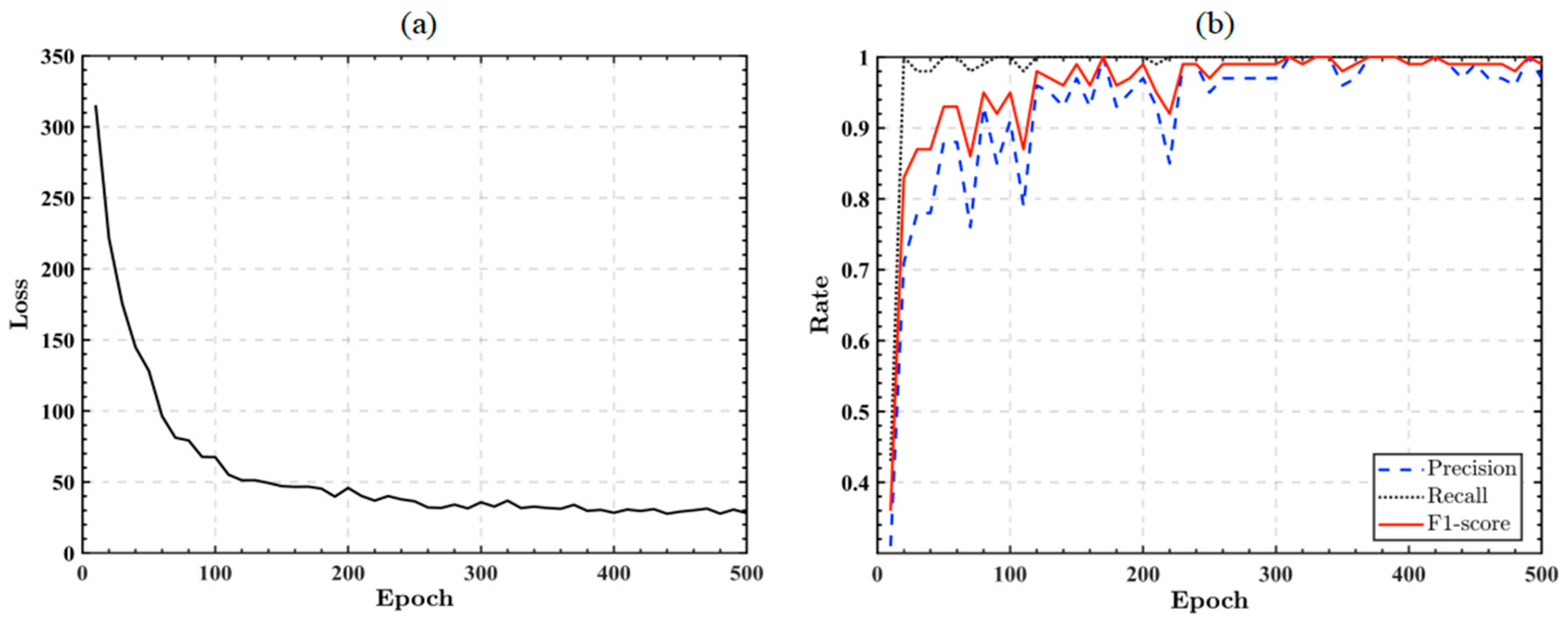
3.3. Network Training

The proposed CGPR2VOX framework was trained using the training dataset for 500 epochs. Crosshole GPR images and permittivity voxel model data pairs were fed into CGPR2VOX with a batch size of 3. The framework calculates the loss function, mean squared logarithmic error (MSLE), in each epoch to evaluate the reconstruction performance. An Adam optimizer is employed to minimize the MSLE and update the weights in the framework, ensuring that training reaches the global optimum. The learning rate, β₁ and β₂ of the optimizer are set to 0.01, 0.9, and 0.999, respectively.

Figure 4a shows the training losses, which represent the MSLE value between the predicted permittivity voxel and the permittivity voxel in the training dataset. The loss value of CGPR2VOX exhibits a sharp decrease before the 100th epoch, gradually converging to a value of 30 at the 500th epoch. This indicates that CGPR2VOX’s ability to reconstruct defects improves progressively as the training advances. We also computed precision, recall, and F1-score to comprehensively evaluate the training effectiveness of defect reconstruction, as shown in Figure 4b. The trends of precision, recall, and F1-score all align with the loss function. CGPR2VOX initially gains the capability to reveal almost all defects in the training dataset by the 10th epoch. Subsequently, the precision of CGPR2VOX’s defect reconstruction steadily increases until the 310th epoch. After training for 500 epochs, precision, recall and F1-score converge to approximately 0.99, demonstrating that the proposed framework is well-trained and capable of accurately reconstructing the defects in the training dataset.

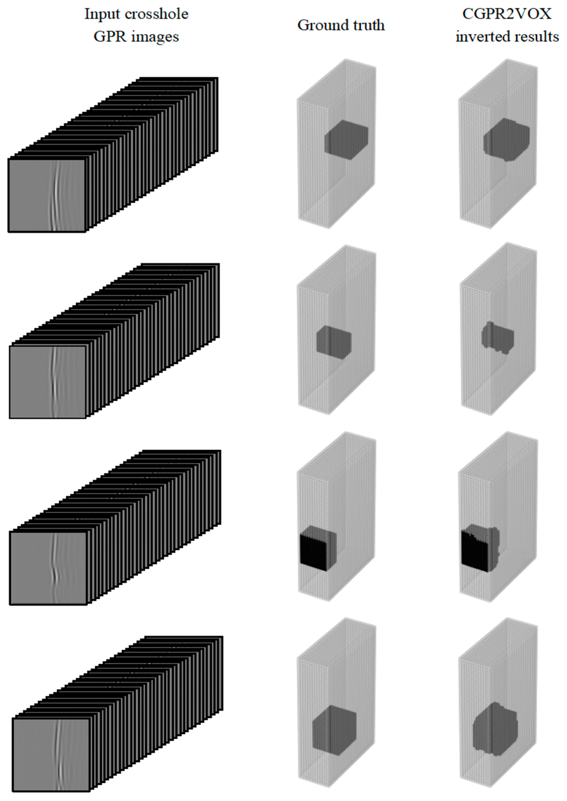
3.4. Reconstruction Accuracy

Next, we evaluated the 3D reconstruction performance of CGPR2VOX on the testing dataset, which contains unseen crosshole GPR images. Figure 5 presents four reconstruction examples in which CGPR2VOX effectively reconstructs the defects in their correct locations and accurately captures their shapes and sizes.

Table 1. Performance evaluation of the proposed 3D reconstruction frameworks.

Evaluation Index		Value
Precision		91.43%
Recall		96.97%
F1-score		94.12%
Mean position error	X-direction	0.86 cm (0.80%)
	Y-direction	0.10 cm (0.09%)
	Z-direction	1.37 cm (1.28%)
Mean processing time		3.70 s
Mean number of artifacts		0.08

summarizes the precision, recall and F1-score of the reconstruction results by CGPR2VOX. Quantitatively, the proposed method achieves a precision of 91.43%, a recall of 96.97%, and an F1-score of 94.12%. These metrics indicate that CGPR2VOX demonstrates robust generalization capabilities when reconstructing unseen crosshole GPR data.

We calculated the average positional errors of the reconstructed defects. This metric quantifies the deviation of the reconstruction defect positions from their true positions in the X, Y, and Z directions. The formula for the average positional error E_pos is the following:

$$E_{\mathrm{pos}}={\displaystyle \frac{1}{N}} {\sum }_{i=1}^N \sqrt{{\left(x_i-x_i^{\prime }\right)}^2+{ \left(y_i-y_i^{\prime }\right)}^2+{ \left(z_i-z_i^{\prime }\right)}^2},$$

(8)

where N is the total number of defects; i denotes the ith defect; (x_i, y_i, z_i) and ($x_i^{\prime }$, $y_i^{\prime }$, $z_i^{\prime }$) are the true and reconstructed coordinates of the defect, respectively. The average positional error in the X-, Y-, and Z-direction are all less than one voxel, measuring 0.86 cm, 0.10 cm, and 1.37 cm, respectively, corresponding to the relative errors of 0.80%, 0.09%, and 1.28%. Meanwhile, our method demonstrates a rapid processing speed for each crosshole GPR data, averaging 3.70 s, while minimizing artifacts to an average of only 0.08 per reconstruction model. Overall, the test results validate the excellent performance of CGPR2VOX in the 3D reconstruction of crosshole GPR images.

3.5. Generalization Ability

In practical engineering scenarios, additional challenges such as varying defect conditions, heterogeneous materials, and diverse sources of EM noise can significantly impact GPR signals. Therefore, it is important to assess the crosshole GPR interpretation method’s ability to resist interference and handle data degradation. In this subsection, we further evaluate the generalization performance of CGPR2VOX by testing its capability to process crosshole GPR data in complex scenarios.

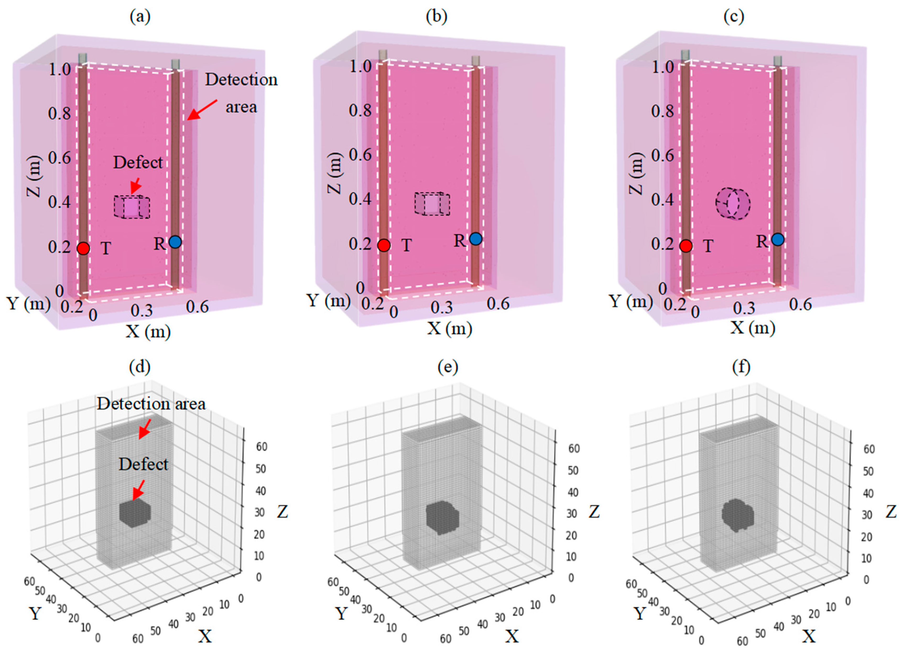
3.5.1. Defect Condition Variations

In the training dataset, defects are simulated using a uniform permittivity value of 80. However, in real retaining walls, the permittivity of defects can vary significantly due to different filling materials. Additionally, the training dataset modeled defects as cube-shaped, whereas actual defects may exhibit various geometries. To evaluate the network’s robustness to variations in permittivity and shape, we conducted generalization tests using data samples with different permittivity values and defect shapes. Notably, the network used for verification is identical to the one trained in Section 3.3 and has not been trained on data with varying permittivity or defect shapes.

Figure 6 presents the verification results under different scenarios. In Figure 6a, the FDTD model is constructed under conditions consistent with the training dataset. Figure 6b shows the FDTD model with the defect permittivity reduced by 50%, and Figure 6c illustrates the FDTD model where the defect is deformed into a cylindrical shape. Figure 6d displays the reconstruction results for data samples that match the training dataset conditions. It can be observed that when the validation data conditions align with the training dataset, the network accurately reconstructs the position, shape, and size of the defects, even though it has not encountered this specific data during training. When the defect permittivity is reduced by 50%, the network still accurately reconstructs the defect, as shown in Figure 6e, demonstrating its generalization capability to variations in permittivity. Furthermore, when the defect shape is deformed into a cylinder, the network not only accurately reconstructs the defect location but also fills the voxels along the defect edges to approximate the cylindrical shape without prior knowledge of cylindrical data samples, as shown in Figure 6f. This indicates that the network can effectively handle variations in defect shapes.

Table 2. Reconstruction performance evaluation under different defect condition scenarios.

Condition	Position Error
	X-Direction	Y-Direction	Z-Direction
Training dataset	0.75 cm (1.25%)	0.16 cm (0.78%)	0.47 cm (0.47%)
Permittivity deviation	0.86 cm (1.42%)	0.55 cm (2.73%)	1.28 cm (1.28%)
Defect deformation	1.09 cm (1.81%)	0.31 cm (1.56%)	0.52 cm (0.52%)

summarizes the quantitative evaluation results of the network’s reconstruction accuracy. Variations in defect permittivity and shape lead to slight increases in reconstruction errors, demonstrating the network’s resilience under altered conditions. The overall low percentage of errors highlights the network’s strong generalization capabilities and its ability to accurately reconstruct defects even when faced with variations not present in the training data. This robustness is crucial for practical applications where defect conditions may be unpredictable and diverse.

3.5.2. Heterogeneous Materials and Noise

To simulate the effect of heterogeneous materials in reinforced concrete on EM waves, we incorporated concrete aggregates and steel reinforcement into the retaining wall model, ensuring structural consistency with those used in the training and testing datasets (shown in Figure 7a). Since the retaining wall model is a reduced-scale simulation, aggregates are represented as randomly sized cubes with side lengths ranging from 1 to 2 cm, while steel reinforcement was modeled as cylinders with a 1 cm diameter. This FDTD model can now simulate the heterogeneous materials found in reinforced concrete retaining walls. Next, we voxelized the detection area to establish a ground truth model, which serves as a benchmark for evaluating reconstruction accuracy, as depicted in Figure 7b.

We then conducted a forward simulation on this FDTD model. Since crosshole GPR data are often contaminated by EM noise, we specifically simulated complex conditions that integrate both equipment and environment noise into the FDTD waveforms. Equipment noise, caused by thermal effects and instabilities within the GPR system, appears as random noise and sporadic high-frequency bursts. We modeled this using Gaussian noise with specific statistical properties (mean: 0, standard deviation: 0.002 for random noise and 0.006 for high-frequency bursts). Environmental noise, influenced by external EM disturbances like radio signals and high-voltage power lines, is simulated using pink noise, which closely mimics the real-world environmental noise spectrum [40]. Figure 8a,b displays examples of the A-scan waveform and B-scan image obtained in this complex scenario, respectively. The presence of steel reinforcement and aggregates causes scattering effects on crosshole GPR signals, altering the shapes of both A-scan and B-scan waveforms. Moreover, EM noise introduces spikes and periodic fluctuations in the A-scan waveforms and creates mosaic-like stripes in the B-scan images.

Despite these complexities that significantly contaminate the crosshole GPR data, CGPR2VOX successfully reveals the correct defect locations, as shown in Figure 8c. The relative position errors of the reconstruction in the X-, Y- and Z-direction are 0.73%, 2.25% and 2.11%, respectively. A slightly greater deviation in the centroid of the reconstructed defect can be observed compared with the evaluation results on the testing dataset. This is primarily attributed to the coupling of scattered waves, EM noise and defect signals across adjacent receiving channels. Such interferences amplify the apparent size of anomalies in B-scan images, leading to an overestimation of the defects’ scale by the network, which results in greater position errors. Notably, no prior knowledge about steel-reinforced concrete or EM noise was introduced to CGPR2VOX during the training, demonstrating its robustness in resisting various disturbances under complex scenarios.

4. Model Experiment

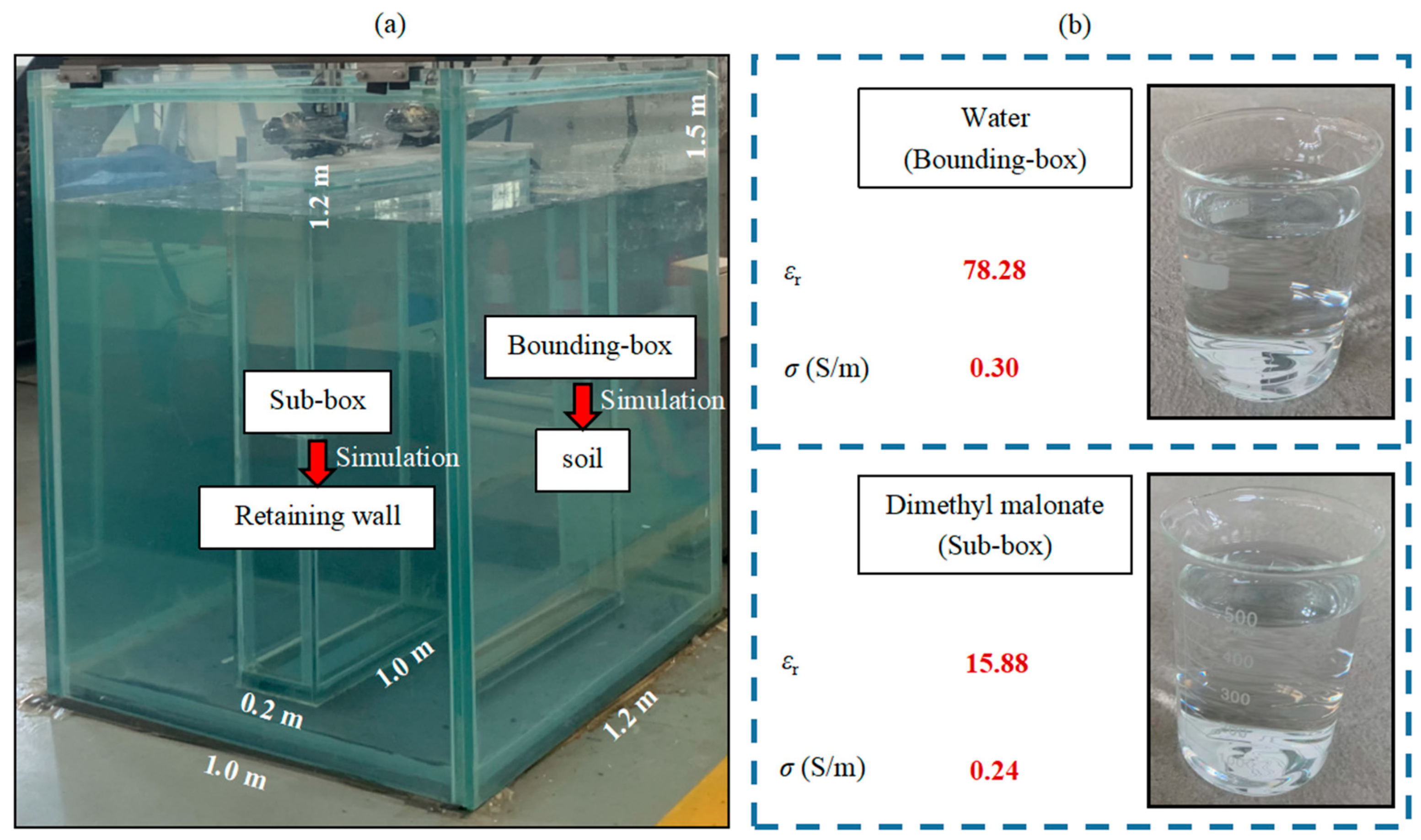
4.1. Experiment System

To verify the feasibility of CGPR2VOX for inverting real-world crosshole GPR data, we designed a novel visual experimental model filled with transparent liquid materials to conduct crosshole GPR measurements. This experiment model simulates underground retaining wall conditions and automatically collects crosshole GPR B-scan images. With this experimental system, defects with arbitrary geometry and dielectric properties can be easily controlled, making the verification more accurate and reliable.

Figure 9a illustrates our experimental system, which includes a step-frequency crosshole GPR and a visible model box designed to simulate the retaining wall and its surrounding soil. Figure 9b provides an exploded view diagram detailing the design of the system. The visible model box consists of a sub-box and a bounding box, which together simulate the detection environment. The pre-fabricated defect model can be securely placed within the sub-box at any desired location. An antenna position control system, implemented with a three-axis synchronous belt slide, is installed on top of the model box. The x-axis and y-axis tracks of the slide align the antennas horizontally with the sub-box and are locked in place to ensure stability during operation. The z-axis tracks control the vertical position of the antennas for data collection inside the sub-box. To achieve precise movements of antennas, we utilized a programmable logic controller (PLC) to automate the control of the z-axis sliders, ensuring a precision of 1 mm. The transmitting and receiving antennas are connected to the crosshole GPR system via coaxial cables, which are fixed to the z-axis sliders. This configuration allows the sliders to move the antennas, enabling automated excitation and collection of EM signals at multiple positions along the z-direction within the sub-box.

4.1.1. Crosshole GPR System

Figure 10 displays the step-frequency crosshole GPR system we developed for data collection. It mainly comprises a vector network analyzer (VNA), a pair of transmitting and receiving antennas, and a laptop computer. The VNA generates an electric signal that is fed to the transmitting antenna, which converts it into electromagnetic signals. The receiving antenna captures the transmitted signals and relays them back to the VNA. The laptop computer controls the entire crosshole GPR system and stores measurement data. By utilizing the crosshole GPR system, accurate data can be collected for further analysis and modeling.

4.1.2. Experiment Model Box

The experiment model box is shown in Figure 11. It consists of a bounding box (1.2 × 1.0 × 1.5 m) and a sub-box (1.0 × 0.2 × 1.2 m), both made of tempered glass. We fill the sub-box with dimethyl malonate (C₅H₈O₄) and the bounding box with water to simulate the relative permittivity difference between the actual retaining wall and the surrounding soil. A time domain reflectometer (TDR) was utilized to determine the permittivity and conductivity of the filling materials. The bounding box contains water with a permittivity of 78.28 and conductivity of 0.30 S/m, while the sub-box contains C₅H₈O₄ with a permittivity of 15.88 and conductivity of 0.24 S/m. This arrangement creates a situation where the EM wave velocity is slower in the bounding box but faster in the sub-box, replicating the behavior of EM waves in actual concrete subsurface structures and the surrounding soil. As a result, the model box designed in this paper can approximate the detection environment of real engineering projects in the laboratory, allowing for flexible defect settings and enhanced visualization.

4.2. Data Acquisition

Figure 12 depicts the data collection using the proposed experimental system. In this experiment, a water-filled defect was placed 0.28 m above the bottom of the sub-box, as shown in Figure 12a. The permittivity and conductivity of the defect are 78.28 and 0.3 S/m, respectively. The transmitting antenna (T) emitted EM waves from 36 positions marked with red dots, covering the height range from 0 to 1 m. Simultaneously, the receiving antenna scanned at a constant speed from 0 to 1 m, collecting EM A-scan waves at 36 positions marked with blue dots. The horizontal distance between the two antennas was maintained at 0.6 m.

Table 3. Experimental data acquisition parameters.

Experimental Parameter	Value
Antenna center frequency	0.78 GHz
Frequence-scanning range	0.65–1.20 GHz
Time window	100 ns
Sampling points for each A-scan	1024
Number of transmitting/receiving points	36
Number of measuring lines	1296
Transmitting/receiving interval	2.86 cm

provides a comprehensive overview of the experimental setup for data acquisition. For data analysis, we combine the A-scan waveforms collected from the 36 measuring lines at various depths into a single B-scan image. The EM waves propagated in these measuring lines all originated from the same position of the transmitting antenna. As a result, we obtained a total of 36 B-scan images, as shown in Figure 12b. It should be noted that these data had not undergone any pre-processing operations, such as energy gain adjustment or filtering. These raw crosshole GPR data were used to be inverted by the trained CGPR2VOX.

4.3. Experiment Results

Finally, we utilized the trained CGPR2VOX model to reconstruct the 3D permittivity voxel from the experimental data. The inverted result is shown in Figure 13. Compared with the ground truth model illustrated in Figure 13a, the CGPR2VOX framework successfully recovers the spatial distribution of the defect. To further validate the superiority of CGPR2VOX, we employed two widely-used crosshole GPR interpretation methods: ray-based tomography and probabilistic FWI [41,42] for comparison. As shown in Figure 13b, ray-based tomography can only perform 2D reconstruction, and the output permittivity image suffers from considerable artifacts. In contrast, Figure 13c demonstrates that probabilistic FWI reconstructs the defect with considerable noise.

Table 4. Reconstruction performance evaluation of the different methods.

Method	Position Error			Number of Artifacts	Processing Time
	X-Direction	Y-Direction	Z-Direction
Proposed method	1.02 cm (1.71%)	0.26 cm (1.32%)	1.30 cm (1.30%)	0	3.73 s
Ray-based tomography	6.71 cm (11.18%)	-	3.27 cm (3.27%)	3	4.59 s
FWI	13.87 cm (23.11%)	0.84 cm (4.18%)	4.26 cm (4.26%)	1	13.05 h

summarizes the reconstruction performances of the three methods. CGPR2VOX achieves reconstruction errors of 1.02 cm, 0.26 cm, and 1.30 cm in the X-, Y- and Z-direction, respectively, with corresponding relative errors of 1.71%, 1.32%, and 1.30%. These results demonstrate a remarkable generalization ability of the proposed method, as the CGPR2VOX model trained with synthetic crosshole GPR data is successfully applied to real-world data interpretation. Quantitative evaluations also indicate that our method significantly outperforms the comparative methods in permittivity reconstruction across all directions and does not produce any artifacts. Furthermore, since the trained CGPR2VOX operates without the parameter iteration typically required in traditional methods, it also has the shortest processing time, demonstrating the comprehensive superiority of our method.

The disparity in reconstruction performance among the three methods is mainly because of the different ways each method utilizes information from crosshole GPR data. Ray-based tomography relies on travel time information, limiting its ability to recover permittivity distributions beyond close proximity to the measuring lines, resulting in imaging artifacts. Probabilistic FWI can incorporate travel time, amplitude, and phase of the GPR waveforms, allowing it to handle 3D reconstruction from crosshole GPR data. However, it is also substantially affected by boarder noise interference. This sensitivity leads to greater reconstruction errors due to the challenges of accurately acquiring the real-world noise distribution. In contrast, our deep learning-based method designs a neural network structure that non-linearly maps full waveform data to a high-dimensional space, enabling the network to effectively learn complex features associated with permittivity distributions. After training, CGPR2VOX can identify meaningful defect signal features and automatically filter out irrelevant noise, ensuring the accuracy of reconstruction results.

5. Conclusions

In this paper, we proposed a GAN-based approach, named CGPR2VOX, for the 3D reconstruction of defects in retaining structures from crosshole GPR data. By integrating a fully connected layer, a residual network, and a specialized 3D decoder in the generator, the crosshole GPR data can be effectively translated into 3D permittivity voxels. After training on a synthetic dataset, it achieved precision, recall and F1-score of 91.43%, 96.97%, and 94.12%, respectively. The defect reconstruction positions exhibit relative errors of 0.80%, 0.09%, and 1.28% in the X-, Y-, and Z-direction, respectively. An experimental model was conducted to verify the applicability of CGPR2VOX to real-world data, yielding relative position errors of 1.67%, 1.65%, and 1.30% in the X-, Y-, and Z-direction, respectively. Our method outperforms commonly used ray-based tomography and probabilistic FWI methods in both speed and accuracy, providing superior permittivity reconstruction results without artifacts. Furthermore, verification in complex scenarios involving reinforced concrete and EM noise demonstrates the framework’s robustness against interference from unseen abnormal signals.

Future work will focus on enhancing the CGPR2VOX framework by incorporating more diverse training data to support the 3D inversion of physical parameters in the detection area. The method will be explored to leverage multimodal information, and it will achieve higher interpretation accuracy in scenarios involving material heterogeneity, complex geometries, and multipath propagation. In addition, CGPR2VOX will be trained on a broader range of defect types, sizes, and materials, improving its generalization across various real-world applications.

References

1. Zhai, J.; Wang, Q.; Xie, X.; Qin, H.; Zhu, T.; Jiang, Y.; Ding, H. A New Method for 3D Detection of Defects in Diaphragm Walls during Deep Excavations Using Cross-Hole Sonic Logging and Ground-Penetrating Radar. J. Perform. Constr. Facil. 2023, 37, 4022065. [Google Scholar] [CrossRef]
2. Wang, J.; Liu, P.; Hu, J.; Pan, W.; Long, Y.; Cao, A.; Li, H.; Sun, Y. Mechanism of Detecting the Construction Quality of a Diaphragm Wall by an Infrared Thermal Field and Engineering Application. Materials 2023, 16, 1052. [Google Scholar] [CrossRef]
3. Zheng, Y.; Chen, C.; Liu, T.; Shao, Y.; Zhang, Y. Leakage Detection and Long-Term Monitoring in Diaphragm Wall Joints Using Fiber Bragg Grating Sensing Technology. Tunn. Undergr. Space Technol. 2020, 98, 103331. [Google Scholar] [CrossRef]
4. Keskinen, J.; Looms, M.C.; Klotzsche, A.; Nielsen, L. Practical Data Acquisition Strategy for Time-Lapse Experiments Using Crosshole GPR and Full-Waveform Inversion. J. Appl. Geophys. 2021, 191, 104362. [Google Scholar] [CrossRef]
5. Wang, S.; Han, L.; Gong, X.; Zhang, S.; Huang, X.; Zhang, P. Full-Waveform Inversion of Time-Lapse Crosshole GPR Data Using Markov Chain Monte Carlo Method. Remote Sens. 2021, 13, 4530. [Google Scholar] [CrossRef]
6. Svendsen, E.B.; Nielsen, L.; Nilsson, B.; Kjær, K.H.; Looms, M.C. Crosshole Ground-Penetrating Radar in Clay-Rich Quaternary Deposits: Towards Characterization of High-Loss Media. J. Geophys. Res. Solid Earth 2023, 128, e2022JB025909. [Google Scholar] [CrossRef]
7. Wang, S.; Han, L.; Gong, X.; Zhang, S.; Huang, X.; Zhang, P. MCMC Method of Inverse Problems Using a Neural Network—Application in GPR Crosshole Full Waveform Inversion: A Numerical Simulation Study. Remote Sens. 2022, 14, 1320. [Google Scholar] [CrossRef]
8. Klotzsche, A.; Vereecken, H.; van der Kruk, J. Review of Crosshole Ground-Penetrating Radar Full-Waveform Inversion of Experimental Data: Recent Developments, Challenges, and Pitfalls. Geophysics 2019, 84, H13–H28. [Google Scholar] [CrossRef]
9. Pereira, M.; Burns, D.; Orfeo, D.; Zhang, Y.; Jiao, L.; Huston, D.; Xia, T. 3-D Multistatic Ground Penetrating Radar Imaging for Augmented Reality Visualization. IEEE Trans. Geosci. Remote Sens. 2020, 58, 5666–5675. [Google Scholar] [CrossRef]
10. van der Kruk, J.; Liu, T.; Mozaffari, A.; Gueting, N.; Klotzsche, A.; Vereecken, H.; Warren, C.; Giannopoulos, A. GPR Full-Waveform Inversion, Recent Developments, and Future Opportunities. In Proceedings of the IEEE 2018 17th International Conference on Ground Penetrating Radar (GPR), Rapperswil, Switzerland, 18–21 June 2018; pp. 1–6. [Google Scholar]
11. Gueting, N.; Vienken, T.; Klotzsche, A.; van der Kruk, J.; Vanderborght, J.; Caers, J.; Vereecken, H.; Englert, A. High Resolution Aquifer Characterization Using Crosshole GPR Full-Waveform Tomography: Comparison with Direct-Push and Tracer Test Data. Water Resour. Res. 2017, 53, 49–72. [Google Scholar] [CrossRef]
12. Mozaffari, A.; Klotzsche, A.; He, G.; Vereecken, H.; van der Kruk, J.; Warren, C.; Giannopoulos, A. Towards 3D Full-Waveform Inversion of Crosshole GPR Data. In Proceedings of the IEEE 2016 16th International Conference on Ground Penetrating Radar (GPR), Hong Kong, China, 13–16 June 2016; pp. 1–4. [Google Scholar]
13. Ernst, J.R.; Green, A.G.; Maurer, H.; Holliger, K. Application of a New 2D Time-Domain Full-Waveform Inversion Scheme to Crosshole Radar Data. Geophysics 2007, 72, J53–J64. [Google Scholar] [CrossRef]
14. Busch, S.; van der Kruk, J.; Bikowski, J.; Vereecken, H. Quantitative Conductivity and Permittivity Estimation Using Full-Waveform Inversion of on-Ground GPR Data. Geophysics 2012, 77, H79–H91. [Google Scholar] [CrossRef]
15. Wang, Z.; Huang, J.; Liu, D.; Li, Z.; Yong, P.; Yang, Z. 3D Variable-Grid Full-Waveform Inversion on GPU. Pet. Sci. 2019, 16, 1001–1014. [Google Scholar] [CrossRef]
16. Deng, J.; Rogez, Y.; Zhu, P.; Herique, A.; Jiang, J.; Kofman, W. 3D Time-Domain Electromagnetic Full Waveform Inversion in Debye Dispersive Medium Accelerated by Multi-GPU Paralleling. Comput. Phys. Commun. 2021, 265, 108002. [Google Scholar] [CrossRef]
17. Mozaffari, A.; Klotzsche, A.; Warren, C.; He, G.; Giannopoulos, A.; Vereecken, H.; van der Kruk, J. 2.5 D Crosshole GPR Full-Waveform Inversion with Synthetic and Measured Data. Geophysics 2020, 85, H71–H82. [Google Scholar] [CrossRef]
18. Zhang, F.; Liu, B.; Wang, J.; Li, Y.; Nie, L.; Wang, Z.; Zhang, C. Two-Dimensional Time-Domain Full Waveform Inversion of on-Ground Common-Offset GPR Data Based on Integral Preprocessing. J. Environ. Eng. Geophys. 2020, 25, 369–380. [Google Scholar] [CrossRef]
19. LeCun, Y.; Bengio, Y.; Hinton, G. Deep Learning. Nature 2015, 521, 436–444. [Google Scholar] [CrossRef]
20. Krizhevsky, A.; Sutskever, I.; Hinton, G.E. Imagenet Classification with Deep Convolutional Neural Networks. Commun. ACM 2017, 60, 84–90. [Google Scholar] [CrossRef]
21. Tjoa, E.; Guan, C. A Survey on Explainable Artificial Intelligence (XAI): Toward Medical (XAI). IEEE Trans. Neural Netw. Learn. Syst. 2020, 32, 4793–4813. [Google Scholar] [CrossRef]
22. Yue, G.H.; Liu, C.L.; Li, Y.S.; Du, Y.C.; Guo, S.L. GPR Data Augmentation Methods by Incorporating Domain Knowledge. Appl. Sci. 2022, 12, 10896. [Google Scholar] [CrossRef]
23. Janiesch, C.; Zschech, P.; Heinrich, K. Machine Learning and Deep Learning. Electron. Mark. 2021, 31, 685–695. [Google Scholar] [CrossRef]
24. Laloy, E.; Linde, N.; Jacques, D. Approaching Geoscientific Inverse Problems with Vector-to-Image Domain Transfer Networks. Adv. Water Resour. 2021, 152, 103917. [Google Scholar] [CrossRef]
25. Laloy, E.; Linde, N.; Ruffino, C.; Hérault, R.; Gasso, G.; Jacques, D. Gradient-Based Deterministic Inversion of Geophysical Data with Generative Adversarial Networks: Is It Feasible? Comput. Geosci. 2019, 133, 104333. [Google Scholar] [CrossRef]
26. Zhang, D.; Wang, Z.; Qin, H.; Geng, T.; Pan, S. GAN-Based Inversion of Crosshole GPR Data to Characterize Subsurface Structures. Remote Sens. 2023, 15, 3650. [Google Scholar] [CrossRef]
27. Isola, P.; Zhu, J.-Y.; Zhou, T.; Efros, A.A. Image-to-Image Translation with Conditional Adversarial Networks. In Proceedings of the 30th IEEE Conference on Computer Vision and Pattern Recognition (CVPR2017), Honolulu, HI, USA, 22–25 July 2017; pp. 5967–5976. [Google Scholar]
28. Ronneberger, O.; Fischer, P.; Brox, T. U-Net: Convolutional Networks for Biomedical Image Segmentation. In Medical Image Computing and Computer-Assisted Intervention–MICCAI 2015: 18th International Conference, Munich, Germany, 5–9 October 2015, Proceedings, Part III 18; Navab, N., Hornegger, J., Wells, W.M., Frangi, A.F., Eds.; Springer International Publishing: Cham, Switzerland, 2015; Volume 9351, pp. 234–241. [Google Scholar]
29. Saad, O.M.; Fomel, S.; Abma, R.; Chen, Y. Unsupervised Deep Learning for 3D Interpolation of Highly Incomplete. Geophysics 2023, 88, WA189–WA200. [Google Scholar] [CrossRef]
30. Guo, P.; Visser, G.; Saygin, E. Bayesian Trans-Dimensional Full Waveform Inversion: Synthetic and Field Application. Geophys. J. Int. 2020, 222, 610–627. [Google Scholar] [CrossRef]
31. Klotzsche, A.; Vereecken, H.; van der Kruk, J. GPR Full-Waveform Inversion of a Variably Saturated Soil-Aquifer System. J. Appl. Geophys. 2019, 170, 103823. [Google Scholar] [CrossRef]
32. Feng, X.; Ren, Q.; Liu, C.; Zhang, X. Joint Acoustic Full-Waveform Inversion of Crosshole Seismic and ground-Penetrating Radar Data in the Frequency Domain. Geophysics 2017, 82, H41–H56. [Google Scholar] [CrossRef]
33. Mirza, M.; Osindero, S. Conditional Generative Adversarial Nets. arXiv 2014, arXiv:1411.1784. [Google Scholar] [CrossRef]
34. Qin, H.; Xie, X.; Vrugt, J.A.; Zeng, K.; Hong, G. Underground Structure Defect Detection and Reconstruction Using Crosshole GPR and Bayesian Inversion. Autom. Constr. 2016, 68, 156–169. [Google Scholar] [CrossRef]
35. Goodfellow, I.; Pouget-Abadie, J.; Mirza, M.; Xu, B.; Warde-Farley, D.; Ozair, S.; Courville, A.; Bengio, Y. Generative Adversarial Nets. Adv. Neural Inf. Process Syst. 2014, 27, 2672–2680. [Google Scholar] [CrossRef]
36. He, K.; Zhang, X.; Ren, S.; Sun, J. Deep Residual Learning for Image Recognition. In Proceedings of the IEEE Conference on Computer Vision and Pattern Recognition, Las Vegas, NV, USA, 26 June–1 July 2016; pp. 770–778. [Google Scholar]
37. Hodson, T.O.; Over, T.M.; Foks, S.S. Mean Squared Error, Deconstructed. J. Adv. Model. Earth Syst. 2021, 13, e2021MS002681. [Google Scholar] [CrossRef]
38. Warren, C.; Giannopoulos, A.; Giannakis, I. GprMax: Open Source Software to Simulate Electromagnetic Wave Propagation for Ground Penetrating Radar. Comput. Phys. Commun. 2016, 209, 163–170. [Google Scholar] [CrossRef]
39. Lin, D. An Information-Theoretic Definition of Similarity. In Proceedings of the Fifteenth International Conference on Machine Learning (ICML’98), Madison, WI, USA, 24–27 July 1998; pp. 296–304. [Google Scholar]
40. Deka, B.; Deka, D. An Improved Multiscale Distribution Entropy for Analyzing Complexity Of-World Signals. Chaos Solitons Fractals 2022, 158, 112101. [Google Scholar] [CrossRef]
41. Hunziker, J.; Laloy, E.; Linde, N. Bayesian Full-Waveform Tomography with Application to Crosshole Ground Radar Data. Geophys. J. Int. 2019, 218, 913–931. [Google Scholar] [CrossRef]
42. Dines, K.A.; Lytle, R.J. Computerized Geophysical Tomography. Proc. IEEE 1979, 67, 1065–1073. [Google Scholar] [CrossRef]
Figure 1. Schematic diagram of the crosshole GPR detection process: (a) antennas setup, (b) wavefield snapshot, (c) waveforms received at multiple depths and (d) final crosshole GPR data block.
Remotesensing 16 03995 g001
Figure 2. Structure of the CGPR2VOX network.
Remotesensing 16 03995 g002
Figure 3. Crosshole GPR dataset preparation for 3D reconstruction.
Remotesensing 16 03995 g003
Figure 4. Evaluation of the training effects of CGPR2VOX: (a) training losses and (b) defect recognition performance.
Remotesensing 16 03995 g004
Figure 5. Example of crosshole GPR 3D permittivity reconstruction on the testing dataset.
Remotesensing 16 03995 g005
Figure 6. Verification results for different defect condition scenarios: (a) FDTD model consistent with the training dataset, (b) FDTD model with a 50% deviation in defect permittivity, (c) FDTD model with cylindrical defect geometry, (d) reconstruction consistent with the training dataset, (e) reconstruction with a 50% deviation in defect permittivity, (f) reconstruction with cylindrical defect geometry.
Remotesensing 16 03995 g006
Figure 7. Numerical simulation for verification in complex scenarios: (a) FDTD simulation, (b) ground truth model.
Remotesensing 16 03995 g007
Figure 8. Results of the forward simulation and defect reconstruction under complex scenarios: (a) A-scan waveform, (b) B-scan image and (c) reconstruction results.
Remotesensing 16 03995 g008
Figure 9. The experimental system: (a) photograph, (b) exploded view diagram.
Remotesensing 16 03995 g009
Figure 10. Step-frequency crosshole GPR system.
Remotesensing 16 03995 g010
Figure 11. Photograph of the model box. (a) Visual effects, (b) measurement results of the electrical parameters of the filling materials.
Remotesensing 16 03995 g011
Figure 12. Crosshole GPR experiment data measurement: (a) photograph of the experiment site, (b) measured B-scan GPR images.
Remotesensing 16 03995 g012
Figure 13. Reconstruction result of the experimental data: (a) photograph of ground truth, (b) result of CGPR2VOX, (c) result of ray-based tomography, and (d) result of probabilistic FWI.
Remotesensing 16 03995 g013