Abstract
While many neural networks have been proposed for hyperspectral image classification, current backbones cannot achieve accurate results due to the insufficient representation by scalar features and always cause a cumbersome calculation burden. To solve the problem, we propose the capsule attention network (CAN), which combines an activity vector with an attention mechanism to improve HSI classification. In particular, we consider two attention mechanisms to improve the effectiveness of the activity vectors. First, an attention-based feature extraction (AFE) module is proposed to preprocess the spectral-spatial features of HSI data, which effectively mines useful information before the generation of the activity vectors. Second, we propose a self-weighted mechanism (SWM) to distinguish the importance of different capsule convolutions, which enhances the representation of the primary activity vectors. Experiments on four well-known HSI datasets have shown our CAN surpasses state-of-the-art (SOTA) methods on three widely used metrics with a much lower computational burden.
1. Introduction
Hyperspectral images (HSIs) contain a wealth of spectral–spatial information within hundreds of continuous spectra, holding promise for distinguishing different land covers at a fine-grained level, particularly for those which have extremely similar spectral signatures in RGB space [1]. Therefore, HSI classification has great potential to effectively achieve a series of high-level Earth observation tasks such as mineral analysis, land cover mapping, precision agriculture, mineral exploration and military monitoring, etc.
Early studies on HSI classification utilized various machine learning-based approaches as feature extractors. Classical methods include K-nearest neighbor [2], Markov random field [3], random forest [4], support vector machine [5] and Gaussian process [6]. These methods can quickly obtain classification results but cannot ensure accuracy since the man-made feature extractor limits the data representation and fitting ability. Thanks to the great success of deep learning, many neural networks have been proposed to achieve HSI classification in an end-to-end way. Neural networks are capable of cultivating the potentially valuable information hiding in the pluralistic data of HSI, and thus have become a ‘hot topic’ in HSI classification [7]. For neural networks, the key problem is how to design the architecture and feature extraction in a way that automatically cultivates high-level nonlinearity features. The Convolutional Neural Network (CNN) is a partularly valuable paradigm, which extracts features by stacking multiple convolutions that have a local receptive field. In an early work, 1-D CNN [8] was proposed to classify HSI by using the spectral signature while ignoring the spatial relation. Subsequently, 2-D CNN was proposed to effectively extract the abundant neighbor information of HSI. Moreover, 3-D CNN [9] can extract features by regarding HSI as various cubes, which takes the spatial information and spectral signature into account simultaneously. Since HSI itself is 3-D data, 3-D CNN outperforms 1-D CNN and 2-D CNN in most cases. Although CNNs have a powerful ability to extract spatially structural and contextual information from HSI, this only works in short-range spatial relation building, and otherwise tends to cause pepper noise [10]. Some recent works [11,12,13] have sought to solve the problem by designing a network architecture and attention mechanism. Although some progress has been made, encoding the local information by scalar features limits the representation ability and causes information loss during the propagation of layers. Some methods, like residual network [14], dense network [15] and frequency combined network [16], can suppress the problem, but they cannot enable CNN-based models to achieve extremely accurate results and always result in a heavy computation burden [17].
Some recent works have helped improve HSI classification performance by designing particular network architectures, including autoencoders (AEs) [18,19], recurrent neural networks (RNNs) [20], graph convolutional networks (GCNs) [21,22,23], Transformers (TFs) [24,25,26], and Mamba [27]. Chen et al. [19] employed stacked AEs to semantically extract spatial–spectral features by considering the local contextual information of HSI. Since it is an unsupervised paradigm, the AE-based method cannot ensure high classification accuracy. Hang et al. [20] designed a cascaded RNN for HSI classification by taking advantage of RNNs to effectively model the sequential relations of neighboring spectral bands. However, RNN can only capture the sequences in short- and middle-dependencies. More recently, more attention has been paid to GCN and TF for HSI classification. GCN regards the pixels as vertices and models the relations of vertices as a graph structure. Therefore, in contrast to GNN, GCN has natural merit for capturing long-range spatial relations [21]. By embedding superpixel segmentation [28], this advantage is further enhanced, avoiding local pepper noise [29]. As a strong substitute for RNN, TF [30] has a powerful ability to build long-term dependencies using a self-attention technique, which has encouraged the development of a large number of TF-based HSI classification models.
However, GCN, TF and Mamba have inevitable limitations due to their intrinsic mechanisms. Although GCN extracts long-range spatial information that ensures the accuracy of non-adjacent patches, the propagation of graph data is still a challenging problem, which restricts the number of GCN layers used and limits deep semantic feature building [31,32]. For TF, it has the merit of building long-range dependency of tokens, and thus has shown huge success in dealing with large-scale datasets in natural language processing [33]. Although TF can be directly used for HSI to build a spectral sequence, its performance is limited by the length of tokens due to relatively fewer “inductive biases” [34]. In other words, in contrast to CNN, TF only builds 2-D information in the MLP layer of Encoder, whose effectiveness is mainly achieved by the self-attention mechanism used [35]. If the token sequence is small, TF will achieve relatively poor performance [36]. Therefore, the performance of TF-based HSI classification methods is limited since the HSI used is generally small- or medium-scale, in which the spectral signature only provides hundreds of tokens, far fewer than TF-based NLP models. On the other hand, although Mamba-based work [27] alleviated the memory burden by using a State-Space Model (SSM) to replace the self-attention mechanism of TF, the classification performance is still limited by the length of the spectral signature.
Many recent works have used composite models to solve the limitations of the current backbones. By “composite” is meant that at least two backbones are combined to compensate mutually for the limitations , thus providing a more exact representation to achieve high-quality classification. For example, CEGCN [37] incorporates the advantages of both CNN and GCN, to jointly cultivate pixel-level and superpixel-level spatial-spectral features to enhance feature representation. WFCG [38] involves a weighted feature fusion model with an attention mechanism, which combines CNN with a graph attention network for HSI classification. Moreover, AMGCFN [39] utilizes a novel attention-based fusion network, which aggregates rich information by merging multihop GCN and multiscale CNN. Moreover, GTFN [40] explores the combination of GCN and TF. By using GCN to provide long-range spatial information, GTFN achieves SOTA performance after using TF for classification. A further approach, DSNet [41], enhances classification performance by introducing a deep AE unmixing architecture to the CNN. The above composite backbones have demonstrated performance improvement resulting from the synergistic effect of the two backbones. However, simply combining two kinds of backbones with a designed fusion strategy only solves the problem of insufficient representation and propagation to a limited extent but results in a huge computational burden.
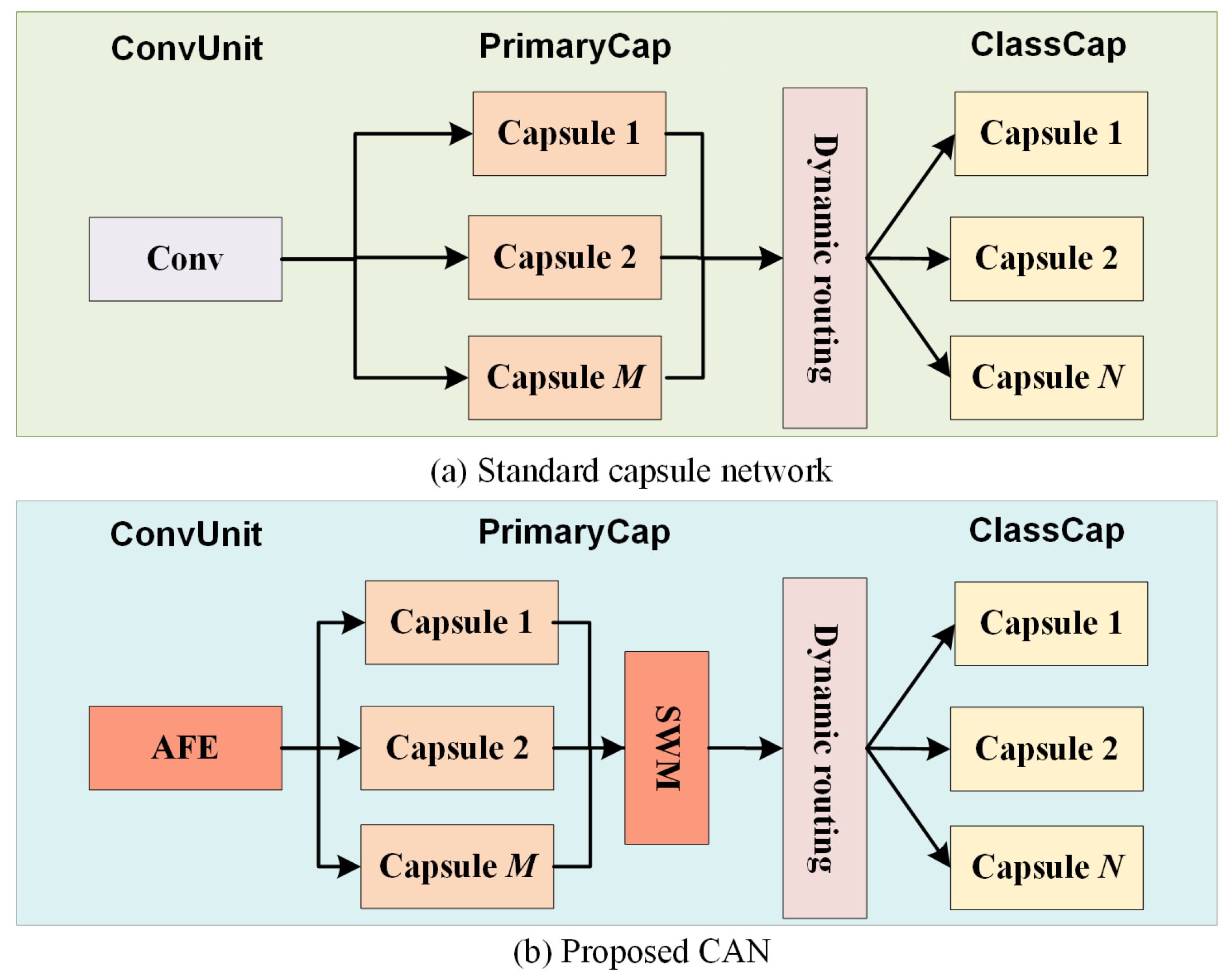
In this paper, we resort to a more abstract feature (activity vector) and rethink HSI classification with a capsule network (CapsNet) [42]. As shown in Figure 1, the pipeline of CapsNet can be divided into three steps termed ConvUnit, PrimaryCap and ClassCap, For standard CapsNet, the ConvUnit contains one convolution, which extracts preliminary features from the data input and sends them to PrimaryCap. PrimaryCap consists of multiple convolutional capsule layers, which are used to yield primary activity vectors. These primary activity vectors are adaptively activated in the ClassCap using a dynamic routing mechanism, and thus obtain the class activity vectors for classification. Some recent works have explored HSI classification based on CapsNet. CNet [43] was the first CapsNet-based model for HSI classification. Subsequently, 3DCNet [44] was proposed, which splits HSI into diverse 3-D cubes as the input to CapsNet to solve the classification problem with limited training samples. More recently, some attention mechanisms have been used to improve the capsule network. For example, SA-CNet [45] encountered a limitation of the ConvUnit step, i.e., a single convolution cannot effectively address the spatial information. Therefore, a correlation matrix with trainable cosine distance was used to assign varying weights for the different patches of HSI. Moreover, ATT-CNet [46] addressed the HSI data using a light-weight channel-wise attention mechanism. It incorporates self-weighted dynamic routing by introducing the self-attention mechanism of Transformer into the activation of the activity vectors. By contrast, our proposed CAN seeks to achieve SOTA classification performance using low-level calculations, and has three obvious differences from recent attention-based capsule networks. First, we drop the spectral signatures by PCA rather than weight them, thus effectively reducing the feature dimension of HSI and improving efficiency. Second, to ensure effectiveness, we design a light-weight module (termed AFE) without distance estimation to adaptively weight each pixel. Moreover, we observed that treating different capsule convolutions equally limits the representation of primary activity vectors. Therefore, we innovatively propose to produce more representative primary activity vectors by adaptively weighting the capsule convolutions during the PrimaryCap step.

Figure 1.
A graphic illustration to show the objectives. (a) The architecture of standard CapsNet. (b) The architecture of the proposed CAN, which provides more rich features in the ConvUnit step and takes the importance of capsules into account.
The main contributions of this research are as follows:
- We propose CAN for HSI classification with two attention components, termed AFE and SWM, which improves the representation of primary activity vectors by, respectively, weighting the pixel-wise features and capsule convolutions in an adaptive way. In contrast to standard CapsNet, our CAN only adds three more convolutions due to the used AFE and SWM, causing insignificant parameter increment. However, benefiting from these attention mechanisms, it can run on an extremely low spectral dimension (with low calculations) of HSI data while achieving much higher classification results.
- We propose AFE block to simultaneously mine spectral–spatial features with an efficient adaptive pixel weighting mechanism, which ensures the ability to gather useful information from HSI data.
- We propose SWM to distinguish the importance of different capsule convolutions, which effectively enhances the representation of primary activity vectors and thus benefits classification performance.
- Experiments on four well-known HSI datasets show our CAN surpasses SOTA methods. Moreover, it is shown that our CAN performs much more efficiently than other methods with an extremely lower computational burden.
The rest of this paper is organized as follows: Section 2 analyzes the limitations of CNN and introduces recent CapsNet based HSI classification works. Section 3 introduces CAN. Section 4 shows the experiments to verify the effectiveness. Section 5 concludes the paper and presents some outlooks for the future.
2. Related Work
2.1. Limitations of CNN for HSI Classification
CNN, as the classical neural network, is a pixel-wise method that extracts high-level semantic representation by stacking diverse convolutions to build the mapping relation. Formally, let the input HSI cube be ; each convolution of the l-th layer computes the dot product between the input and weight matrix as
where denotes the kernel size and s denotes the stride. and denote the input data and the weight of element . is the corresponding output after convolution. is the bias. Therefore, the obtained will be an array of scalar values.
The size of the kernel and stride are essential for convolution. The kernel is a statistical property of the image, which can be considered as a stationary reflection of the pixel area, where the pixels are equally distributed with corresponding positions. The stride denotes the scan interval of the kernel. Therefore, convolution in essence numeralizes the local information of the input, and thus deeper convolution has a larger receptive field, which extracts more semantic features [47]. As the representation limitation of scalar features, CNN always needs a multiscale and deep network with a large number of convolutions and nonlinear layers to ensure the effectiveness, which creates difficulties for the feature propagation between long-range layers. Although some classical frameworks like ResNet or DenseNet ensure effective feature flow, the huge calculation burden still cannot be met on computing-constrained devices. More importantly, the limited representation of scalar presents a bottleneck to HSI classification.
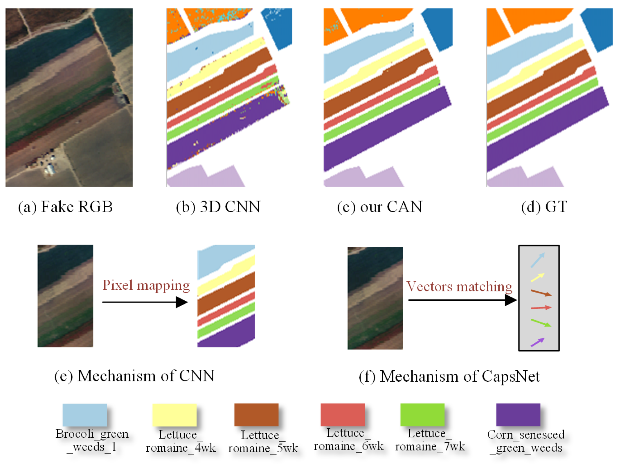
Although extracting the spatial and spectral information simultaneously, 3-D CNN [9] still cannot achieve exact classification. As can be seen in Figure 2, 3-D CNN causes much pepper noise within the area that has obvious context relations. This error stems from the insufficient representation of the scalar feature for complex and mixed HSI information. Fortunately, it is easy to address such limitations by using CapsNet. Different from CNN, CapsNet establishes a vector feature transmission mechanism and outputs a series of class activity vectors, where the number of vectors strictly equals the number of land cover types. Therefore, instead of building pixel mapping in scalar form (for CNN), CapsNet aims to find a specific entity by representation of the activity vector, where the length of the vector denotes the likelihood that the current pixel belongs to this entity. The activity vector provides a more exact representation since it covers multi-dimensional features, where each dimensionality focuses on certain properties of the entity. These properties can include any type of parameter, such as position, orientation, size, hue, albedo, texture, etc. [42], which provides sufficient information to consider how the pixels are spatially arranged.
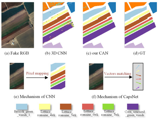
Figure 2.
A graphic illustration to show the internal mechanism of CNN and CapsNet. Due to the pixel mapping achieved by the scalar feature, 3-D CNN creates much pepper noise. In contrast, CapsNet finds a series of activity vectors, where each vector represents one kind of entity in the input while the vector length determines the confidence. Since each vector covers rich information on the diverse properties of the entity with a controllable vector dimension, CapsNet yields a more abstract and exact representation pattern than CNN. In this way, our CAN obtains much better results that are very similar to GT.
2.2. CapsNet for HSI Classification
CapsNet provides a more abstract feature presentation for HSI data, and can achieve SOTA classification with a lower parameter and calculation burden than other backbones. There are some HSI classification models based on CapsNet. For example, an early work, CNet [43], extended CapsNet for HSI classification. 3DCNet [44] was proposed to split HSI into diverse 3-D cubes as the input and included a three-dimensional dynamic routing algorithm to exploit the spectral–spatial features during the ClassCap step. Moreover, some recent works have introduced attention mechanisms to improve CapsNet-based HSI classification. SA-CNet [45] includes a spatial attention mechanism in the ConvUnit step, where a correlation matrix with a trainable cosine distance function is used to assign varying weights for different cubes of HSI. ATT-CNet [46] improved CapsNet-based HSI classification models by using two attention mechanisms. First, in the ConvUnit step, it deals with the HSI data using a light-weight channel-wise attention mechanism, which highlights the useful spectral information. In the Classcap step, ATT-CNet uses the self-attention mechanism of Transformer for dynamic routing, which improves the effectiveness of some useful primary activity vectors. More recently, TSCCN [48] was proposed involving a two-stream spectral-spatial convolutional capsule network, where an efficient structural information mining module (SIM) is designed to learn complementary cross-channel attention between two streams. Our proposed CAN aims to achieve SOTA classification with limited calculation by introducing a reasonable attention module into the ConvUnit and PrimaryCap steps, which is different from recent HSI classification works that combine an attention mechanism with CapsNet. In the ConvUnit step, different from ATT-CNet and SA-CNet, we first use PCA to drop the spectral dimension to one-fifth of the HSI data and then design a light-weight spatial attention mechanism (not relying on distance calculation like SA-CNet) to weight the HSI cubes. Moreover, this is the very first work to consider the attention of capsule convolutions during the generation of the primary activity vectors. The unique attention mechanism enables our CAN to achieve SOTA classification with far fewer calculations by only using one-fifth of the spectral dimensions of HSI data.
3. CAN
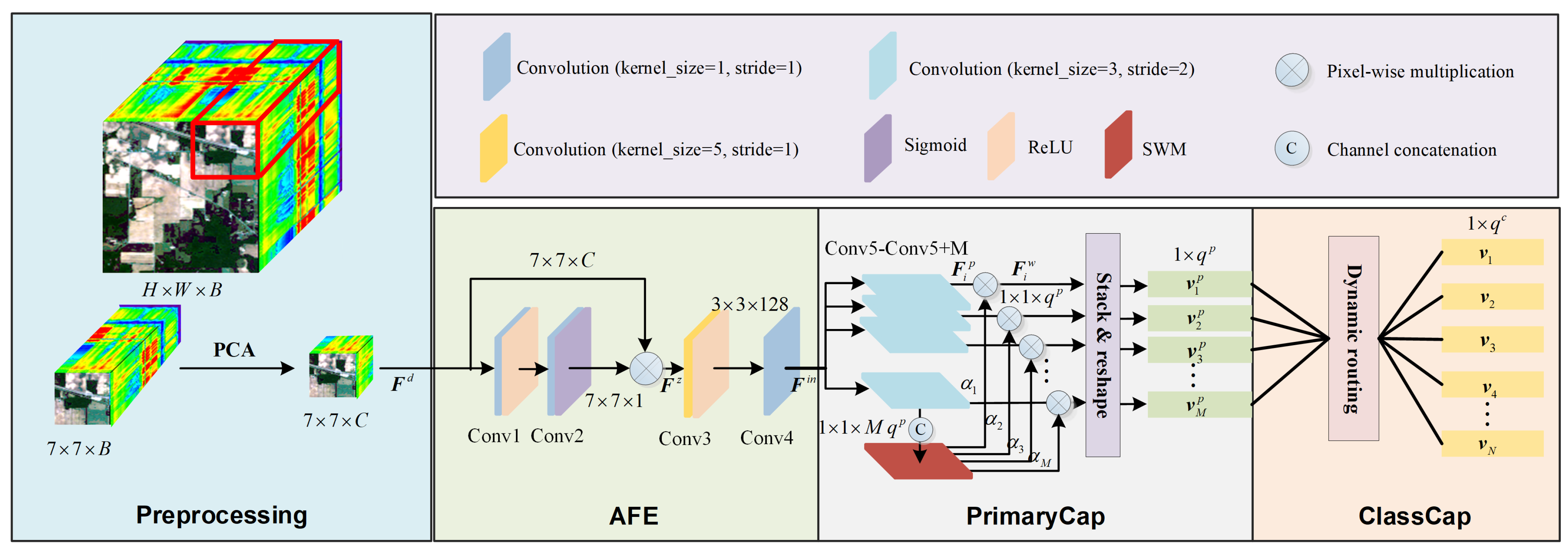
The pipeline of CAN can be divided into four steps termed Preprocessing, ConvUnit, PrimaryCap and ClassCap. As can be seen in Figure 3, the Preprocessing step extracts spectral-spatial information from HSI. Assuming the dimension of HSI is , where H, W and B denote the values of height, width and band, respectively. First, we randomly extract a spectral-spatial cube with a patch size of 7. Afterwards, inspired by [19,24], we drop the spectral band from B to C using a classic dimensionality reduction method, PCA. By projecting into orthogonal space, PCA adaptively finds valuable spectral features (i.e., principal components). In our experiments, we set , which reduces redundant information to improve efficiency while maintaining effectiveness. Moreover, the remaining three steps are the standard pipeline of CapsNet. However, we propose AFE for the ConvUnit step to weight the different pixels in an adaptive way. Moreover, a novel attention mechanism is designed in the PrimaryCap step to automatically distinguish the importance of capsule convolutions. We next detail the three steps.
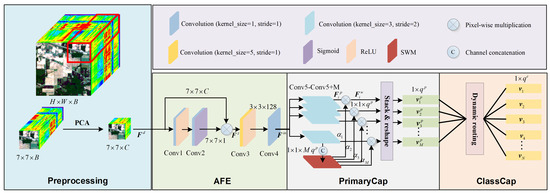
Figure 3.
The overall framework of the proposed CAN.
3.1. AFE
Standard CapsNet utilizes a single convolution to process the input data, which uses all information equally and fails to gather useful features. Therefore, we propose AFE, a simple but effective module to quickly obtain high-quality features. Attention mechanisms are a widely studied topic in recent works [12,24,45,46]. The famous Squeeze-and-Excitation Network [49] (SENet) is in essence a channel-wise attention, which has been verified to be effective in improving the classification task. Moreover, CBAM [50] (Convolutional Block Attention Module) and DBDA [12] (Double-Branch Dual-Attention) were proposed to benefit from channel- and spatial-wise attention, which fuse the weighted features in a cascaded and parallel way, respectively. The proposed AFE is different from the above works since it only uses spatial-wise attention, and no channel-wise attention is used. This design is because PCA discards most bands, which means the remaining spectral bands are all important and adding channel-wise attention only achieves a quite limited gain. Concretely, the output of prepossessing is first sent to a convolution (kernel size 1, stride 1) with the ReLU function to obtain the nonlinearity features. After that, another convolution (kernel size 1, stride 1) with the sigmoid function is used to yield a spatial-wise attention map by dropping the channel dimension to 1. This process can be mathematically defined as
where denotes the output of preprocessing. and denote the first and second convolution, respectively. denotes the adaptively learned pixel-wise attention map. As can be seen from the angle of spatial attention, the proposed AFE is also different from CBAM and DBDA. First, in contrast to the spatial attention in CBAM, the proposed AFE obtains the spatial attention map by two convolutions with a ReLU function rather than by one convolution. The addition of one convolution with the ReLU function enhances the ability to build nonlinear features, making the attention mechanism more efficient with negligible computational increment. Moreover, in contrast to the spatial attention in DBDA, the proposed AFE only learns the attention map in one branch rather than in three branches, which ensures efficiency. In particular, the convolution’s kernel size of AFE is pixel-wise (1 × 1) rather than having a large kernel size (7 × 7 and 9 × 9) as used in CBAM and DBDA, respectively, which fits in pixel classification. After learning the attention map, we obtain the weighted features as
where ⊗ denotes element-wise multiplication. denotes the weighed features by pixel-wise attention. Hereto, we have obtained more representative features by distinguishing the importance of each pixel in an automatic way.
After spatial-wise attention, it is necessary to conduct nonlinearity mapping again to extract the high-level features and adjust the scale. To be specific, a convolution (kernel size 5, stride 1) with ReLU function is used to change the patch size from to . To suppress the loss of spatial information, we correspondingly increase the channel dimension to 128. Finally, these features are sent to another convolution (kernel size 1, stride 1) to accomplish the feature preparation for the PrimaryCap step.
3.2. PrimaryCap
The PrimaryCap step yields primary activity vectors, which are the lowest level of multi-dimensional entities. Here, the concept of entity can be understood as land covers (i.e., classification objects) with multi-dimensional parts of interest that are expressed as the instantiation parameters [42]. These instantiation parameters are meaningful; for HSI, they represent the associated properties of the corresponding land-cover type. Therefore, in this sense, the generation of the capsule can be interpreted as being opposite to the rendering process in computer graphics, where the pattern is obtained by applying rendering to an object with corresponding instantiation parameters.
The PrimaryCap is an M-dimensionality convolutional capsule layer with channels, i.e., it contains M capsule convolutions with the kernel size being 3 and the stride being 2. Therefore, in total, PrimaryCap obtains M capsules, where each output is a dimensionality vector. This process can be mathematically defined as
where denote the M capsule convolutions. are the extracted features. Considering the outputs of all the M capsules, we stack them in dimension 0 to obtain . Afterwards, is reshaped as , where M denotes the number of activity vectors and denotes the vector dimension. From another angle, M is also the number of parallel convolutions and denotes the corresponding number of output channels. In our experiments, we set and .
After obtaining the vectors, a squash operation should be conducted, which serves as the nonlinearity mapping operation of the vector version. The mathematical definition is
where denotes the obtained primary activity vectors after the squash operation. From another angle, Equation (7) can also be regarded as a weight operation of the vector. First, it is easy to see denotes the normalized vector of . Based on this, the larger the norm of , the more the norm of gets closer to 1. While the less the norm of , the more the norm of gets closer to 0. This shows Equation (7) is meaningful, which makes these vectors well recognized.
Equations (4)–(7) show the pipelines of the standard CapsNet. It is easy to see that the learned primary activity vectors are closely related to the M capsules. A natural idea is to automatically give the importance of these capsules and thus improve the representation of the primary activity vectors. Therefore, a simple but effective method, termed SWM, is designed to adaptively yield the weights. Concretely, we concatenate all the in the channel dimension and then send them into SWM to generate the weights for all the capsules by a gated convolution. This process can be mathematically denoted as
where denotes the concatenation operation in channel dimensionality. is a convolution with kernel size of 3, with stride of 1, and thus it only changes the size of the channels. The input channel is and the output channel is M, which can be regarded as the adaptive weight maps of M capsules. Formally, the weighted features can be defined as
where are the weighted features. Afterwards, Equations (5) and (6) are solved sequentially to obtain high-quality activity vectors. These activity vectors are further squashed by Equation (7) to obtain primary activity vectors for the ClassCap step.
It is easy to see the proposed SWM is meaningful. First, since the input of is the concatenated features of all the capsules, it is theoretically explainable that the output M maps can give reasonable weights for the results of different capsules. Moreover, the SWM has two obvious advantages. On the one hand, the weights are data driven, free from manmade priors. On the other hand, in contrast to the standard capsule network, it only introduces one more convolution, and thus the added calculation quantity can be completely ignored.
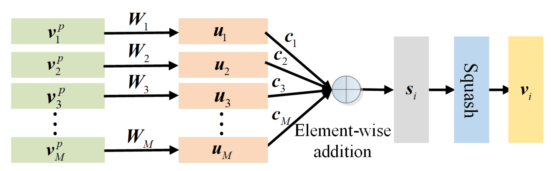
3.3. ClassCap
The ClassCap step describes an information propagation rule between vectors. Following [42], we use dynamic routing to build such relations. As shown in Figure 4, the primary activity vectors are first transformed by a projection matrix as
where denotes the projected vectors. These vectors are weighted by different weights and fused by element-wise addition. The process can be mathematically defined as
where denotes the n-th weighed vector, where n denotes the number of class activity vectors (also the number of land cover types). Afterwards, the squashing operation (Equation (7)) is conducted on to obtain the class activity vector . Assuming the total iteration number of dynamic routing is T, the weight is adaptively updated by

Figure 4.
Graphical illustration of dynamic routing.
In Equation (13), denotes the weight at the epoch, where denotes the index of iteration. According to [42], we set in the experiments. · denotes the inner-product, which is used to estimate the similarity of the two vectors. Since denotes the fused vector, the weighting mechanism is meaningful since the vector input with a more positive contribution will be incrementally assigned a larger weight. The whole process is summarized in Algorithm 1.
| Algorithm 1: Dynamic routing. |
|
3.4. Loss Function
The margin loss and reconstruction loss are used to train the proposed CAN.
where L denotes the overall loss, and and denote the margin loss and reconstruction loss, respectively. is a trade-off for the loss, which is suggested as 0.0005 [42].
(1) Margin Loss: For a CapsNet, it is expected that the class capsule for entity c will have a long instantiation vector if, and only if, that entity is present in the current input. Therefore, the margin loss is used as
where if the current input is assigned to class c with margin coefficients and . stops the initial learning from shrinking the lengths of the activity vectors of all the class capsules, which is suggested as 0.5 [42].
(2) Reconstruction Loss: The reconstruction loss is used as a regularization to ensure exact pattern representation for each entity. If the current entity belongs to class capsule c, we first mask the outputs of all other class capsules and then only use the result of capsule c to reconstruct the input. The reconstruction network is composed by three fully connected layers as follows:
where denotes the fully connected layers. and are followed by a ReLU function; while is followed by a sigmoid function. The reconstruction loss is defined as
where denotes loss.
4. Experiments and Discussion
Section 4.1 introduces the used hyperspectral datasets. Section 4.2 introduces the experimental setting and implementation details. Section 4.3 shows the experimental results. Section 4.4 presents the ablation study.
4.1. Data Description
During the experiments, well-known hyperspectral datasets are used. They are Indian Pines (IP), Salina (SA), Pavia University (PU), UH2013 and UH2018.
The IP dataset is captured from scenes in northwestern Indiana by the AVIRIS sensor, and contains 145 × 145 pixels and 224 bands. By removing some interference bands, 200 bands remain. This dataset contains 10,249 labeled pixels with 16 feature categories in total. In our experiments, 435 samples are selected as training data and 9814 samples as testing data. The division of samples is shown in Table 1. As can be seen, our division strategy may result in the training samples being less than the testing samples (e.g., Class 9) due to the extremely uneven distribution of IP. The classification results of this class can verify the performance where there are sufficient training samples.

Table 1.
Category information of IP dataset.
The SA dataset is captured from scenes in the Salinas Valley, California by the AVIRIS sensor, which contains 512 × 217 pixels and 224 bands. By removing some interference bands, 204 bands remain. This dataset contains 54,129 labeled pixels with 16 feature categories in total. In our experiments, 480 samples are selected as training data and 53,649 samples as testing data. The division of samples is shown in Table 2.
Table 2.
Category information of SA dataset.
The PU dataset is captured from scenes from Pavia university, and contains 610 × 340 pixels and 115 bands. By removing some interference bands, 103 bands remain with 9 feature categories and 42,776 labeled pixels. In our experiments, 270 samples are selected as training data and 42,506 samples as testing data. The division of samples is shown in Table 3.
Table 3.
Category information of PU dataset.
The UH2013 dataset has a size of 349 × 1905, with 144 effective bands, 15 land cover classes, and a spatial resolution of 2.5 m. In our experiments, 450 samples are selected as training data and 14,579 samples as testing data. The division of samples is shown in Table 4.
Table 4.
Category information of UH2013 dataset.
UH2018 is a large-scale dataset, which has a size of 601 × 2384 with 50 effective bands and 20 land covers. In our experiments, 600 samples are selected as training data and 504,256 samples as testing data. The division of samples is shown in Table 5.
Table 5.
Category information of UH2018 dataset.
4.2. Experiment Settings
(1) Implementation Details of CAN: Our CAN was implemented on the PyTorch 1.12 framework using a PC with one RTX 2080Ti GPU. For the training of CAN, we set the patch size as , and used PCA to drop the band dimensionality as of the HSI input. The total epoch is set at 300 with an initial learning rate of . After each ten epochs, the learning rate is decreased to nine-tenths of the latest learning rate. The batch size is set as 128, and the Adam [51] optimizer is utilized.
(2) Comparison With the SOTA Backbones: We compare our CAN with 13 representative deep learning HSI classification methods to comprehensively verify its effectiveness. These methods are as follows: the CNN-based methods, 3-D CNN [9], RSSAN [11], DBDA [12]; the GCN-based method MDGCN [22]; the capsule-based methods CNet [43], ATT-CNet [46], SA-CNet [45]; the TF-based methods SSFTT [24], GAHT [25], SF [26]; the Mamba-based work MHSI [27] and the composite methods WFCG [38], AMGCFN [39], GTFN [40], and DSNet [41]. Among the composite methods, WFCG and AMGCFN combine the merits of CNN and GCN to improve HSI classification. GTFN combines the merits of GCN and TF to enhance classification performance. For all the comparative methods, we directly use the published model by the authors with the suggested parameter settings and training epochs. All the experiments were conducted on the same PC with one RTX 2080Ti GPU.
(3) Evaluation Metrics: Three widely used metrics, the Overall classification Accuracy (OA), the Average classification Accuracy (AA), and the Kappa coefficient are chosen to quantitatively verify the performance. Moreover, qualitative analysis is simultaneously carried out by visualizing the classification maps.
4.3. Experiment and Analysis
(1) Quantitative Analysis: Table 6, Table 7, Table 8 and Table 9 show the quantitative results of the IP, SA, PU and UH2013 datasets, respectively. For the CNN-based methods, 3-D CNN obtains relatively lower results. By combining spectral–spatial attention, RSSAN improves the performance to some extent, but the results are still much lower than for other works. It is interesting that by designing a double-branch dual-attention mechanism, DBDA achieves competitive results. The results show that CNN-based methods are limited by the inadequate representation of scalar features, whose effectiveness relies on the design of the network architecture and attention mechanism. By contrast, MDGCN utilizes multi-scale dynamic graph convolution to improve classification, which achieves results that are near to those for CNN-based DBDA. Moreover, it seems that the performance of TF-based methods is limited to some extent. First, like 3-D CNN, SF simply uses the spectral–spatial information for Transformer, which obtains much lower results than the same type methods SSFTT and GAHT. For SSFTT, the performance improvement mainly results from using the Gaussian weighted feature tokenizer. For GAHT, a more complex group-aware hierarchical transformer is used, and the performance is usually better than SSFTT. All the results show that TF-based methods hit the same bottleneck as the CNN-based method, i.e., the baseline cannot achieve accurate classification due to insufficient feature representation and thus it relies on a well-designed architecture or attention mechanism. Examining the results of the composite models WFCG, AMGCFN, GTFN and DSNet, we can see that the metrics are generally higher than for those that only use one backbone. Interestingly, as can be seen in the 9th class of the IP dataset, we find that all the methods except WFCG achieve 100% accuracy. This demonstrates that WFCG is unstable and cannot ensure high accuracy under sufficient training samples. Moreover, combining GCN with TF (GTFN) achieves significant advantages when compared with methods that incorporate CNN and TF (WFCG and AMGCFN). However, by only using the standard CapsNet, CNet achieves SOTA results. Moreover, the attention-based CapsNet ATTCNet and SA-CNet obtain much better results than all the recent attention-based CNN methods, TF or composite models. The results show that CapsNet better fits HSI classification by using high-level abstract vector features to represent entity patterns. Consistently better than all other methods, our CAN obtains the best results on these four datasets by using a suitable attention mechanism to address HSI data and improve the primary activity vectors.
Table 6.
Quantitative comparison on IP dataset. Numbers in bold denote the best value in comparison to others.
Table 7.
Quantitative comparison on SA dataset. Numbers in bold denote the best value in comparison to others.
Table 8.
Quantitative comparison on PU dataset. Numbers in bold denote the best value in comparison to others.
Table 9.
Quantitative comparison on UH2013 dataset. Numbers in bold denote the best value in comparison to others.
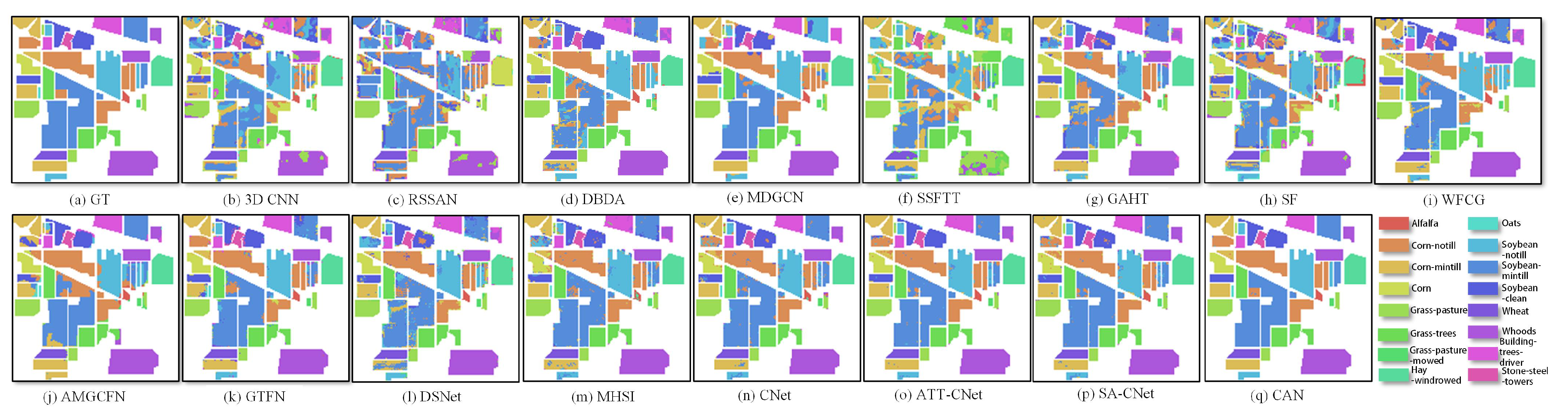
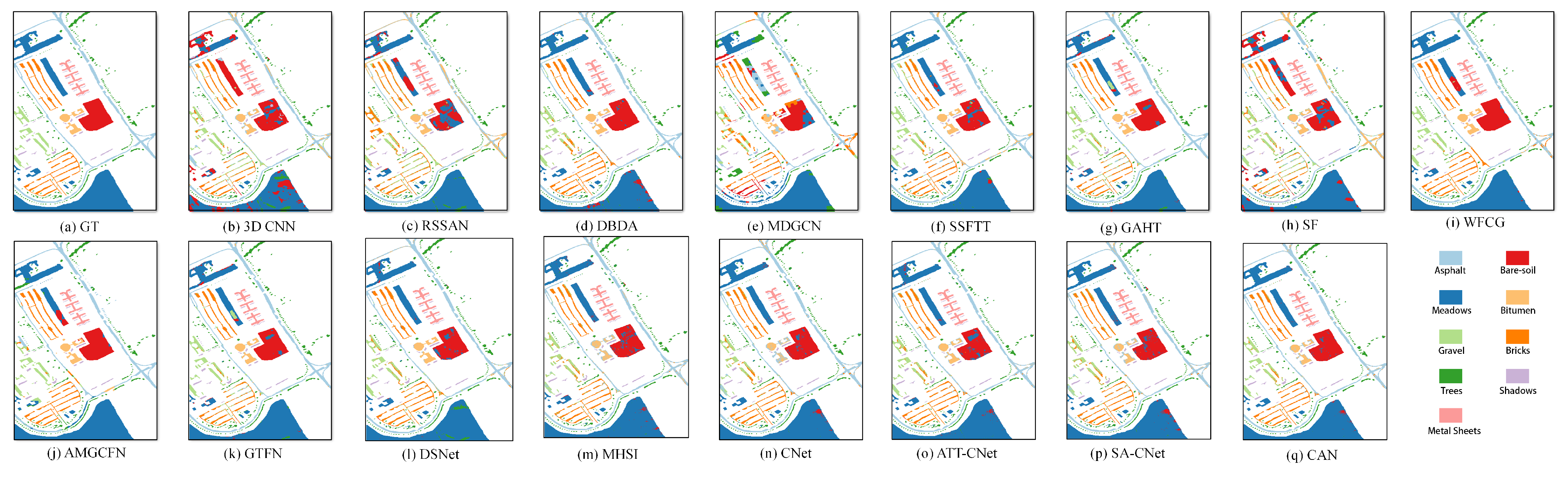
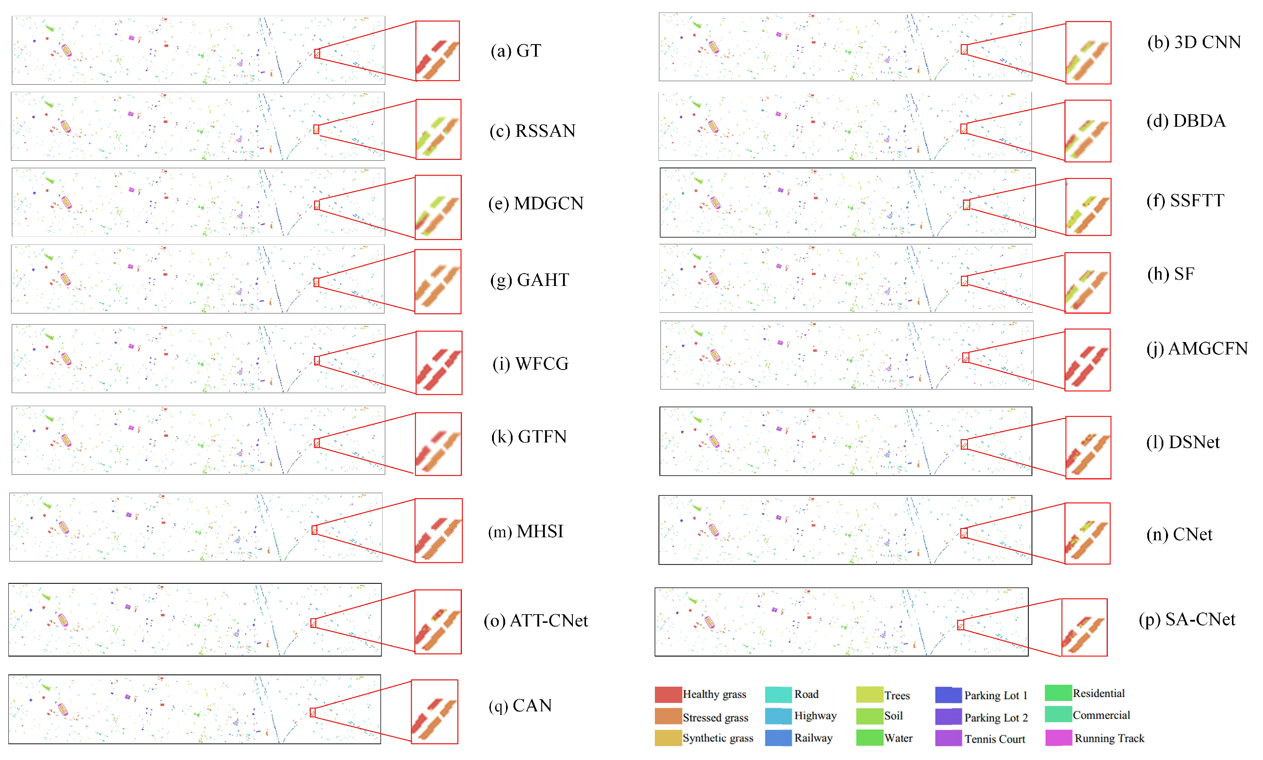
(2) Visual Analysis: This section qualitatively analyzes the performance of different methods using visual maps. Figure 5, Figure 6, Figure 7 and Figure 8 show the results of IP, SA, PU and UH2013, respectively. In all the datasets, the CNN-based method 3-D CNN, and the TF-based methods SSFTT and SF, do not work well, leading to a large amount of pepper noise and even large patches of false classification. Moreover, the CNN-based methods RSSAN and DBDA tend to cause many false results within or on the edges of entities. Although the GCN-based method MDGCN effectively builds the long-range spatial relation using a superpixels graph, some clumpy misclassification can be found. A similar problem can be seen in the maps of the TF-based method GAHT. The Mamba-based work MHSI causes obvious dotted noise. All the results show that the current backbones fail to achieve accurate classification due to inefficient feature representation. A composite model can be used to solve the problem to some extent. As can be seen, the CNN and GCN composite methods WFCG and AMGCFN produce better maps, where the false classification is effectively suppressed. AE and the CNN composite method DSNet result in some pieces of noise. By contrast, the GCN and TF composite method GTFN outperforms the other composite methods by using the long-range spectral dependencies (TF) and long-range spatial relations (GCN) simultaneously. Although some progress has been made, a large number of false classification can be found in the results of the composite methods. By contrast, CNet achieves competitive visual maps when compared to these composite methods. By using spatial attention for the HSI data, SA-CNet ameliorates the false classification to some extent. The visual maps of ATT-CNet are smoother than that of SA-CNet by introducing attention for the activation of the activity vectors. Better than all other methods, the proposed CAN achieves the most smooth visual map. In particular, for the IP dataset, we can see the visual map of CAN very closely approximates that of GT. For UH2013, the proposed CAN restores the details more exactly for some similar regions (e.g., the healthy grass and the stressed grass in the amplified areas of the red boxes) than the recent attention-based CapsNet models ATT-CNet and SA-CNet.
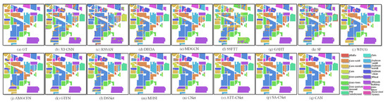
Figure 5.
Visual maps of the results on the IP dataset.
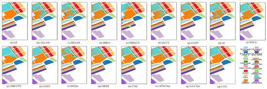
Figure 6.
Visual maps of the results on the SA dataset.
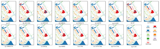
Figure 7.
Visual maps of the results on the PU dataset.
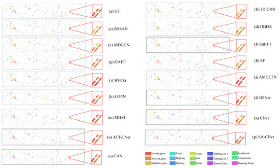
Figure 8.
Visual maps of the results on the UH2013 dataset.
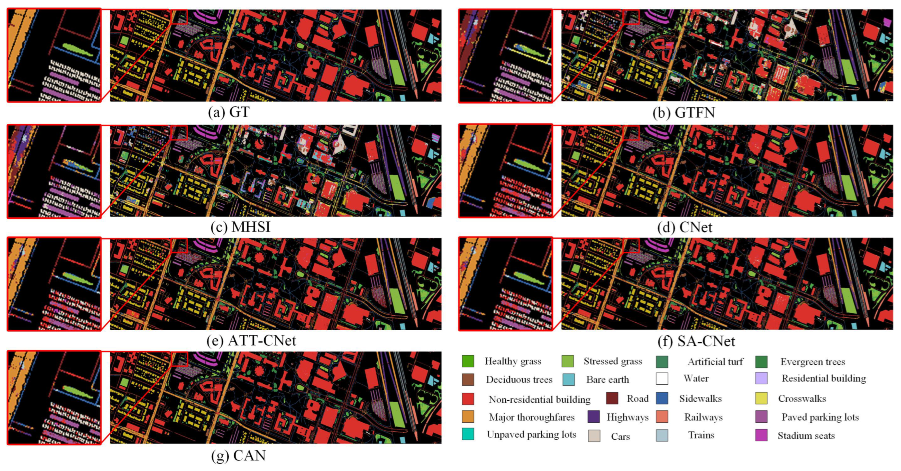
(3) Experiments on UH2018. To verify generalization of the ability to challenge a large-scale dataset, we tested on UH2018. The comparative methods include the composite model GTFN, the Mamba-based model MHSI, and the CapsNet-based models CNet, ATT-CNet, SA-CNet. All of these are quite recently proposed models that have shown strong competitiveness against our CAN according to the results on the previous four benchmarks. We report both quantitative and qualitative results. For the quantitative results, we run each method two times and report the average values. Table 10 reports the results. As can be seen, our CAN still achieves SOTA classification with all three metrics’ results being much higher than those of the comparative methods. In particular, examining the results of Class 9, it is found that the CapsNet-based methods obtain much higher accuracy. Since we only use 30 samples for training and test the classification results on 223,722 samples, GTFN and MHSI obtain much lower accuracy for this class. The results show that the CapsNet-based methods have better ability to achieve accurate classification when the number of training samples is quite limited, which has been verified by previous work [44]. Moreover, we note that our CAN performs much better than other CapsNet-based models on Class 3 and Class 17, but it still fails to exactly classify Class 12 (i.e., Crosswalks).
Table 10.
Quantitative comparison on UH2018 dataset. Numbers in bold denote the best value in comparison to others.
We further show the visual maps in Figure 9. As can be seen, the CapsNet-based methods achieve much more exact results than other backbones for Class 9 (non-residential buildings). Moreover, in the amplified box, we find that the CapsNet-based methods all achieve a smoother map for Class 13 (major thoroughfares). However, they tend to cause false classification on complex areas where there is adjacent location of residential buildings and water. By using AFE and SWM to enhance the representation of HSI data and primary activity vectors, our CAN obtains a much better map for this region against the other attention-based CapsNet models ATT-CNet and SA-CNet.
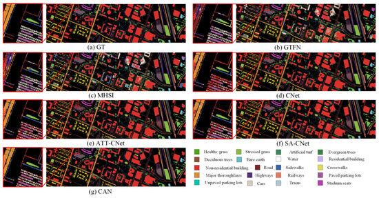
Figure 9.
Visual maps of the results on the UH2018 dataset.
(4) Training Samples Analysis: To further verify the effectiveness and stability of the proposed CAN, we draw the curves of OA using different proportions of the training samples. As shown in Figure 10, to control the number of training samples, we set the diverse proportions of the training samples as 1%, 2%, 3%, 4%, 5% if the total samples are less than 20,000, otherwise 0.25%, 0.5%, 1%, 2%, 3%. Concretely, the proportions of the training samples for the rIP and UH2013 datasets were set as . The proportions of the training samples for the SA, PU and UH2018 datasets were set as . The results show that the OA of the different algorithms are generally increased as the training samples increase since the model can be adequately trained with more training samples. Among all the algorithms, CAN always acquires the best OA when using different proportions of samples for the training on these datasets, which demonstrates its excellent and stable performance. in particular, for the large-scale dataset UH2018, our CAN outperforms other methods by a large margin, which demonstrates its ability to achieve high classification accuracy for challenging data. More importantly, when the proportion of training samples are relatively small, our CAN provides a much higher OA than the competitors, which shows the stability of our CAN when the number of training samples is limited. All the results show that the proposed AFE and SWM effectively improve the quality of the activity vectors, providing an exact representation for each entity enabling CAN to obtain accurate classification even for extremely limited training conditions.
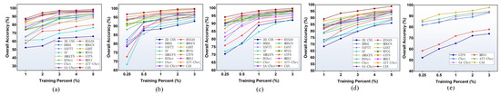
Figure 10.
OA curves for different proportions of training samples on the datasets. (a) IP. (b) SA. (c) PU. (d) UH2013. (e) UH2018.
(5) Efficiency Analysis: To verify the efficiency, we recorded the time cost and computational burden (FLOPs) of the different methods. The results are reported in Table 11. As can be seen, recent works built a complex network to improve classification, resulting in a large time cost and computational burden. This disadvantage is aggravated when a multi-scale architecture (e.g., MDGCN) or composite mode is used (e.g., WFCG and AMGCFN). Based on an entirely different approach, capsule networks learn an exact representation using activity vectors, enabling them to achieve SOTA classification results with an extremely simple architecture. Therefore, CNet relies on few calculations with 0.34 G FLOPs. By combining CapsNet with an attention mechanism, ATT-CNet and SA-CNet increase the calculation quantity to some extent but this is still much lower than for most recent works. Better than all the other methods, the proposed CAN needs a much lower calculation quantity of 0.18 G FLOPs since it only uses spectral signatures to achieve SOTA classification, which means our CAN needs much less time to yield the classification results, especially when tested on large-scale datasets (as can be seen in the time cost on UH 2018). Our CAN can achieve SOTA by using limited spectral signatures due to the unique attention design for HSI data and the primary activity vectors. The huge merits of accuracy and efficiency demonstrate that our CAN has wide industrial application prospects.
Table 11.
Results of efficiency experiments. Numbers in bold denote the best value. Default unit is second. “m” and “h” denote minute and hour, respectively.
4.4. Ablation Experiment and Model Analysis
(1) Ablation Experiment for Overall Framework: For our CAN, three modules termed PCA, AFE and SWM are proposed to reduce the calculation and enhance the classification performance of CapsNet. To explore the contribution of them, this part reports an ablation experiment on the IP dataset. The results are reported in Table 12. As can be seen, using the standard CapsNet achieved high results on all the three metrics, only slightly lower than some recent SOTA methods. By distinguishing the contribution of pixels, the proposed AFE effectively improves the feature representation of HSI data, which increases all the metrics especially when using PCA to achieve classification with a limited spectral dimension. More importantly, the proposed SWM makes an appealing improvement by enhancing the primary activity vectors with a self-taught mechanism. By using both of them, the proposed method achieves somewhat better results. In particular, it can be seen that although PCA dramatically reduces the calculation of the proposed CAN, it drops the performance to some extent. Fortunately, with the proposed AFE and SWM, our proposed method obtains the second-best results, only slightly lower than those generated without using PCA. Therefore, we prefer to use PCA for accelerating our proposed method. All the three components enable our proposed CAN to achieve SOTA performance with extremely little calculation.
Table 12.
Results of ablation experiment.
(2) The Study of AFE: The proposed AFE plays an important role in improving the classification performance. Therefore, we explore its effectiveness in this part. First, we compare AFE with the spatial attention mechanism used in DBDA [12] and CBAM [50]. The results are reported in Table 13. As can be seen, using AFE achieves the best results. Compared with DBDA, it it is seen that using multi-branches to obtain the attention map is not necessary. Compared with CBAM, our AFE effectively improves the OA from 96.74 to 97.91 since the introduced convolution and ReLU enhance the feature-building ability. Moreover, like CBAM, we also performed an experiment using channel-wise attention (CA) before AFE. The results show a quite limited gain. A main reason is that PCA has discarded most bands, which means that the remaining bands are all important and it is not necessary to weight them.
Table 13.
Results by comparing AFE with other attention mechanisms.
The kernel size of AFE was studied further. As can be seen in Table 14, the results show that using a smaller kernel generates better OA. A very possible reason is that HSI classification is a pixel classification task. Therefore, using 1 × 1 kernel better weights the pixels.
Table 14.
Results by changing the kernel size of AFE.
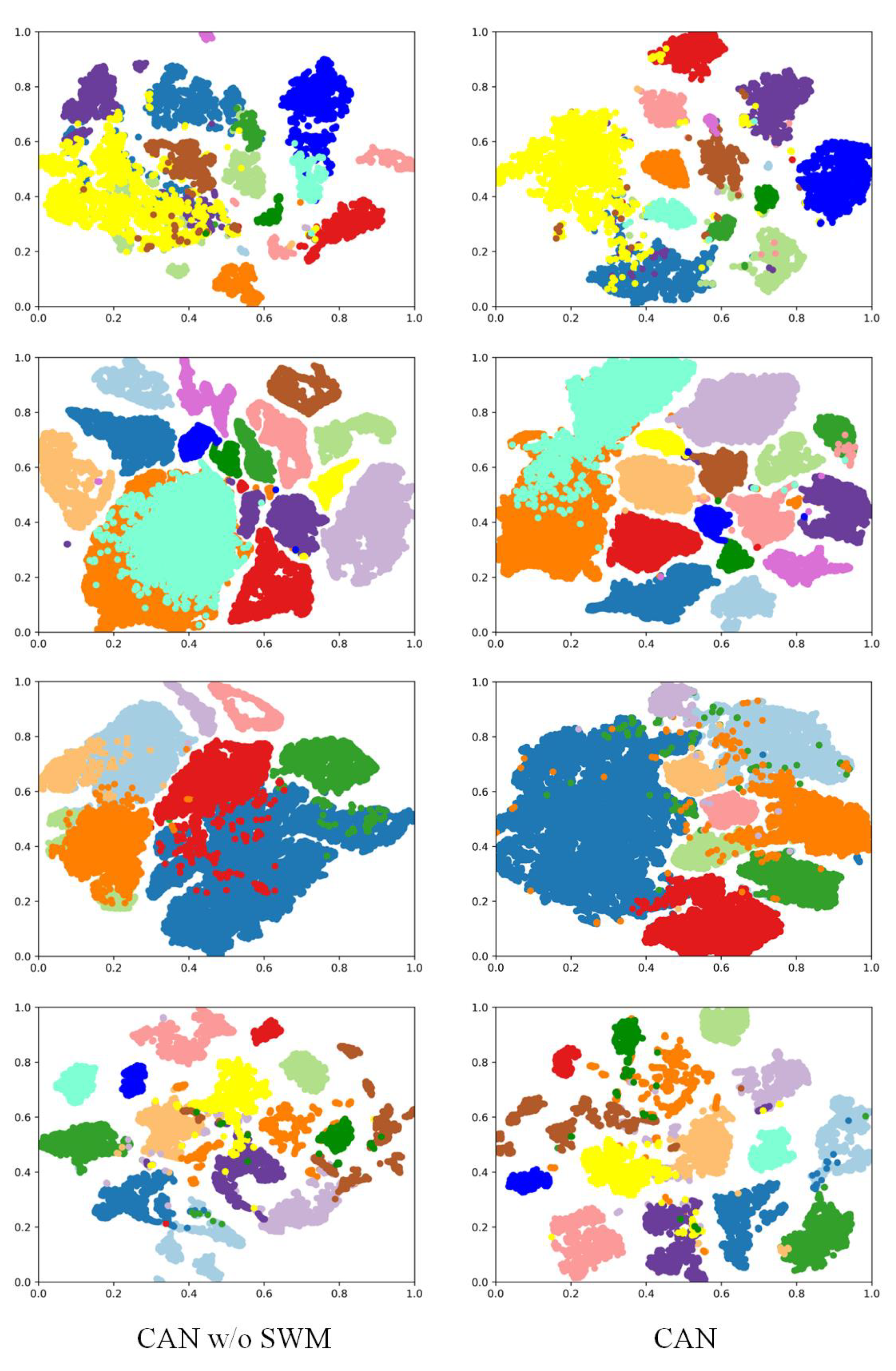
(3) The Study of AWM: The proposed AWM is designed to adaptively weight different capsule convolutions, thus generating primary activity vectors with more effective representation. In this part, we show that using AWM makes the learned features more discriminative. We use t-sne to show the feature distribution with (w/o) SWM. The results are shown in Figure 11. As can be seen, after using SWM, the proposed CAN learns more compact features on all the datasets, which results in improved classification performance. Therefore, weighting the capsule convolutions is a feasible approach to improving the performance of CapsNet.
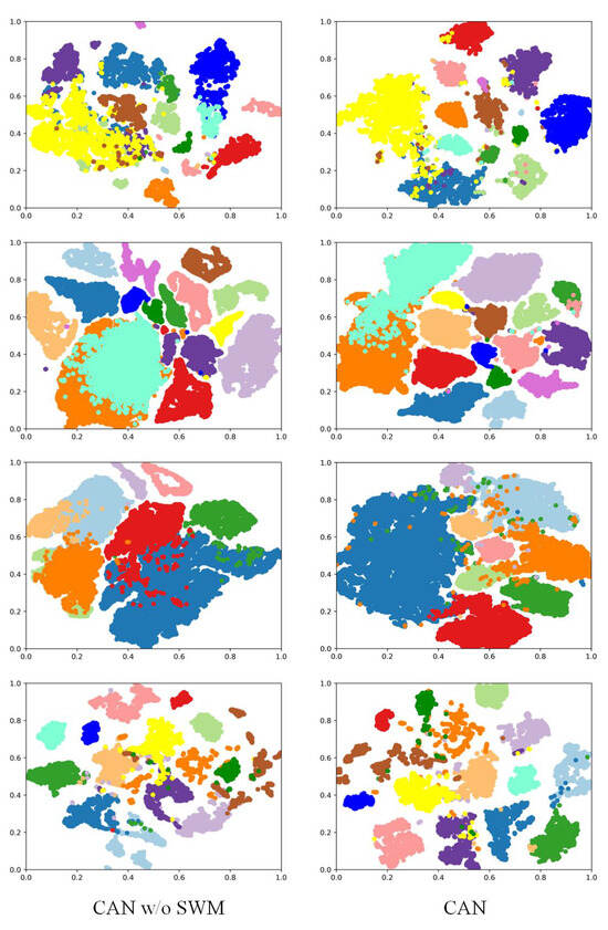
Figure 11.
The visual feature distributions using t-sne. From the first row to the fourth row, the results of AP, SA, PU, UH2013, respectively, are shown.
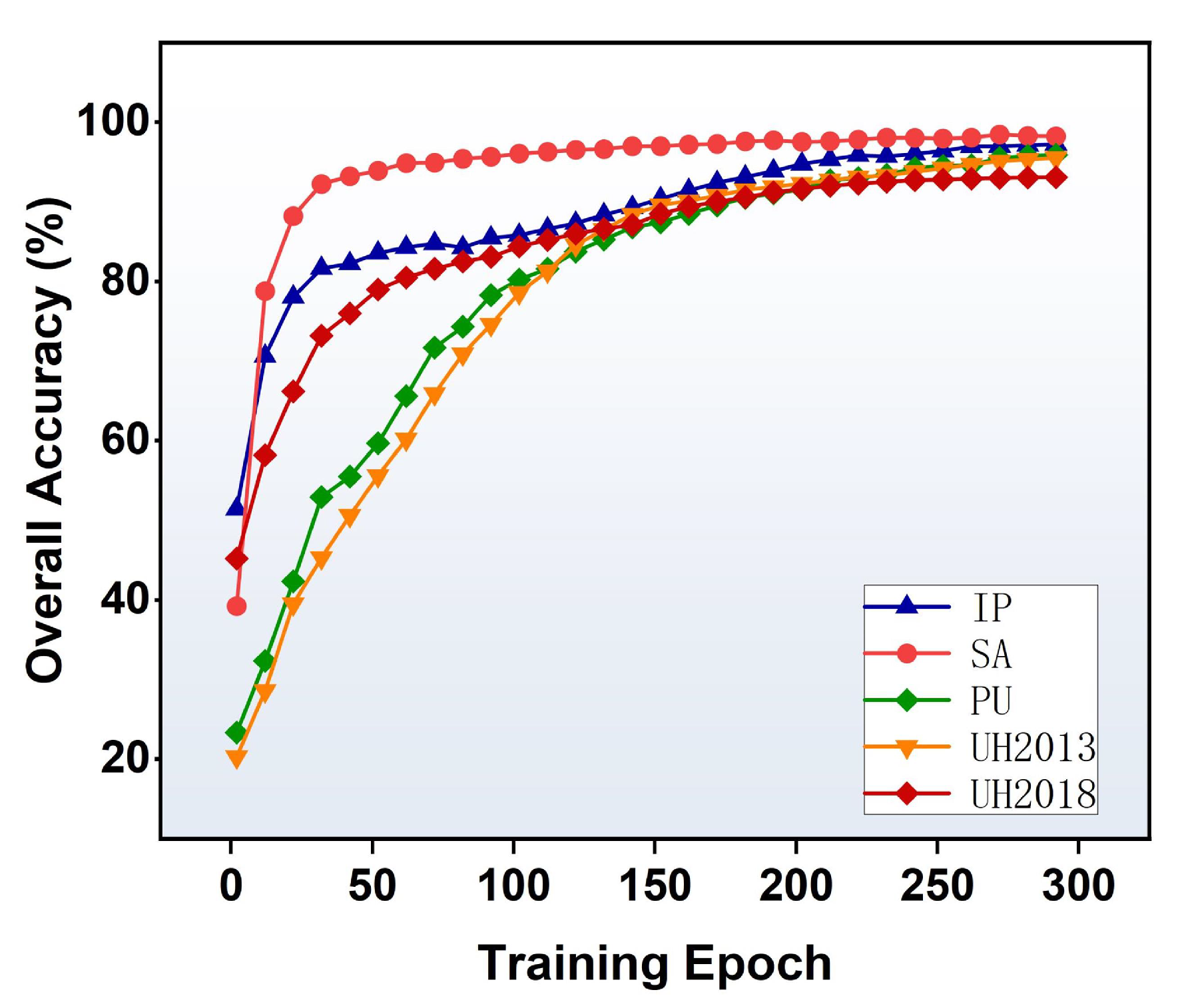
(4) Intermediate Result Analysis: How fast can the proposed CAN achieve satisfactory classification results is an interesting question. To analyze the problem, the OA curves are drawn with the recorded values after each 10 epochs. As can be seen in Figure 12, for the SA dataset, our CAN stably obtains a high OA value after 100 epochs; while for the IP, PU and UH2013 datasets, it obtains a high OA value after 200 epochs. These intermediate results show that our CAN is highly efficient, being free from large iterations for data training. In particular, although the UH2018 dataset is large, we find that our CAN improves the performance faster than when tested on PU and UH2013, with nearly 80% OA after 50 epochs. Therefore, we set the total training epoch as 300. Compared with the SOTA HSI classification methods, this represents an obvious advantage since many other methods [24,26,27,41] need more than 500 epochs for training, and some (e.g., [22]) need even more than 1000 epochs.
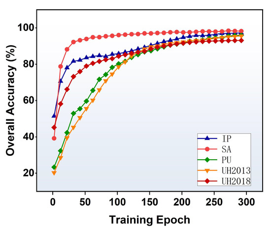
Figure 12.
OA curves on the datasets.
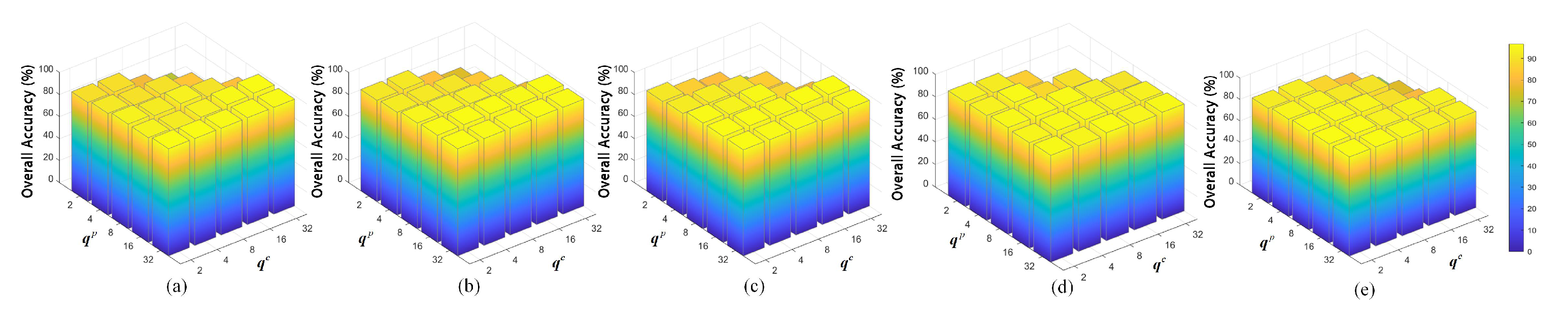
(5) Sensitivity Analysis of the Vector Dimension: For our CAN, the dimensions of the primary activity vector and the class activity vector are key variables, which should be set in advance. To analyze the sensitivity of these two variables, a grid searching strategy is used. The results are shown in Figure 13. As can be seen, the classification performance (OA) is not sensitive to the setting of these two vector dimensions. However, readers should note that the dimension of the primary activity vector () should set a larger value than that of the class activity vector (). Otherwise the performance might be dropped to a low value. should be regarded as incorrect settings since more property features cannot be produced out of thin air when conveying the information of the activity vectors.

Figure 13.
Sensitivity analysis for the dimensions of the primary activity vector () and the class activity vector () on the datasets. (a) IP. (b) SA. (c) PU. (d) UH2013. (e) UH2018.
5. Conclusions
This paper proposes CAN, a capsule attention network for HSI classification. By using activity vectors, our CAN yields more abstract and exact representations for entities. To fully cultivate the advantage of CapsNet, AFE is proposed to extract rich and useful features from spatial-spectral input. Furthermore, SWM is subtly designed to better yield primary activity vectors by self-weighting all the capsule convolutions, which ensures high-quality class activity vectors for entity representation. Experiments on the HSI datasets showed that our CAN surpasses 13 SOTA methods by a large margin with a much lower time cost and computational burden.
Author Contributions
Conceptualization, N.W.; methodology, N.W.; validation, N.W. and A.Y.; formal analysis, N.W. and A.Y.; writing—original draft, N.W. and Z.C.; writing—review and editing, Z.C., Y.D., Y.X. and Y.S.; supervision, Y.S.; project administration, Y.S.; funding acquisition, Z.C. and Y.S. All authors have read and agreed to the published version of the manuscript.
Funding
This work was supported in part by the Natural Science Foundation of Shaanxi Province under Grant 2020JQ-298 and 2023-JC-YB-501.
Data Availability Statement
The original data presented in the study are openly available and we also provide them with the code of CAN. The code will be published at https://github.com/NianWang-HJJGCDX/CAN.git (accessed on 23 October 2024).
Acknowledgments
The authors would like to thank D. Landgrebe at Purdue University for providing the free downloads of the Indian Pines and Salinas datasets, and P. Gamba from the University of Pavia for providing the Pavia University dataset.
Conflicts of Interest
The authors declare no conflicts of interest. The founding sponsors had no role in the design of the study; in the collection, analyses, or interpretation of data; in the writing of the manuscript; nor in the decision to publish the results.
References
- Zhang, H.; Liu, H.; Yang, R.; Wang, W.; Luo, Q.; Tu, C. Hyperspectral Image Classification Based on Double-Branch Multi-Scale Dual-Attention Network. Remote Sens. 2024, 16, 2051. [Google Scholar] [CrossRef]
- Guo, Y.; Han, S.; Li, Y.; Zhang, C.; Bai, Y. K-nearest neighbor combined with guided filter for hyperspectral image classification. In Procedia Computer Science; Elsevier: Amsterdam, The Netherlands, 2018; pp. 159–165. [Google Scholar]
- Zhang, B.; Li, S.; Jia, X.; Gao, L.; Peng, M. A daptive Markov random field approach for classification of hyperspectral imagery. IEEE Geosci. Remote Sens. Lett. 2011, 8, 973–977. [Google Scholar] [CrossRef]
- Amini, S.; Homayouni, S.; Safari, A.; Darvishsefat, A.A. Object-based classification of hyperspectral data using random forest algorithm. Geo-Spat. Inf. Sci. 2018, 21, 127–138. [Google Scholar] [CrossRef]
- Melgani, F.; Bruzzone, L. Classification of hyperspectral remote sensing images with support vector machines. IEEE Trans. Geosci. Remote Sens. 2004, 42, 1778–1790. [Google Scholar] [CrossRef]
- Li, W.; Prasad, S.; Fowler, J.E. Hyperspectral image classification using Gaussian mixture models and Markov random fields. IEEE Geosci. Remote Sens. Lett. 2013, 11, 153–157. [Google Scholar] [CrossRef]
- Islam, M.R.; Islam, M.T.; Uddin, M.P.; Ulhaq, A. Improving Hyperspectral Image Classification with Compact Multi-Branch Deep Learning. Remote Sens. 2024, 16, 2069. [Google Scholar] [CrossRef]
- Hu, W.; Huang, Y.; Wei, L.; Zhang, F.; Li, H. Deep convolutional neural networks for hyperspectral image classification. J. Sens. 2015, 2015, 258619. [Google Scholar] [CrossRef]
- Ben Hamida, A.; Benoit, A.; Lambert, P.; Ben Amar, C. 3-D Deep Learning Approach for Remote Sensing Image Classification. IEEE Trans. Geosci. Remote Sens. 2018, 56, 4420–4434. [Google Scholar] [CrossRef]
- Jia, S.; Jiang, S.; Zhang, S.; Xu, M.; Jia, X. Graph-in-Graph Convolutional Network for Hyperspectral Image Classification. IEEE Trans. Neural Networks Learn. Syst. 2024, 35, 1157–1171. [Google Scholar] [CrossRef]
- Zhu, M.; Jiao, L.; Liu, F.; Yang, S.; Wang, J. Residual spectral–spatial attention network for hyperspectral image classification. IEEE Trans. Geosci. Remote Sens. 2020, 59, 449–462. [Google Scholar] [CrossRef]
- Li, R.; Zheng, S.; Duan, C.; Yang, Y.; Wang, X. Classification of hyperspectral image based on double-branch dual-attention mechanism network. Remote Sens. 2020, 12, 582. [Google Scholar] [CrossRef]
- Ding, Y.; Zhang, Z.; Zhao, X.; Cai, W.; Yang, N.; Hu, H.; Huang, X.; Cao, Y.; Cai, W. Unsupervised self-correlated learning smoothy enhanced locality preserving graph convolution embedding clustering for hyperspectral images. IEEE Geosci. Remote Sens. 2022, 60, 5536716. [Google Scholar] [CrossRef]
- Zhang, X.; Shang, S.; Tang, X.; Feng, J.; Jiao, L. Spectral partitioning residual network with spatial attention mechanism for hyperspectral image classification. IEEE Geosci. Remote Sens. 2021, 60, 5507714. [Google Scholar] [CrossRef]
- Ahmad, M.; Khan, A.M.; Mazzara, M.; Distefano, S.; Roy, S.K.; Wu, X. Hybrid dense network with attention mechanism for hyperspectral image classification. IEEE J. Sel. Top. Appl. Earth Obs. Remote Sens. 2022, 15, 3948–3957. [Google Scholar] [CrossRef]
- Yang, A.; Li, M.; Wu, Z.; He, Y.; Qiu, X.; Song, Y.; Du, W.; Gou, Y. CDF-net: A convolutional neural network fusing frequency domain and spatial domain features. IET Comput. Vision 2023, 17, 319–329. [Google Scholar] [CrossRef]
- Xue, Y.; Jin, G.; Shen, T.; Tan, L.; Wang, N.; Gao, J.; Wang, L. SmallTrack: Wavelet pooling and graph enhanced classification for UAV small object tracking. IEEE Trans. Geosci. Remote Sens. 2023, 61, 5618815. [Google Scholar] [CrossRef]
- Ding, Y.; Zhang, Z.; Zhao, X.; Cai, Y.; Li, S.; Deng, B.; Cai, W. Self-Supervised Locality Preserving Low-Pass Graph Convolutional Embedding for Large-Scale Hyperspectral Image Clustering. IEEE Geosci. Remote Sens. 2022, 60, 5536016. [Google Scholar] [CrossRef]
- Chen, Y.; Lin, Z.; Zhao, X.; Wang, G.; Gu, Y. Deep Learning-Based Classification of Hyperspectral Data. IEEE J. Sel. Top. Appl. Earth Obs. Remote Sens. 2014, 7, 2094–2107. [Google Scholar] [CrossRef]
- Hang, R.; Liu, Q.; Hong, D.; Ghamisi, P. Cascaded Recurrent Neural Networks for Hyperspectral Image Classification. IEEE Trans. Geosci. Remote Sens. 2019, 57, 5384–5394. [Google Scholar] [CrossRef]
- Hong, D.; Gao, L.; Yao, J.; Zhang, B.; Plaza, A.; Chanussot, J. Graph Convolutional Networks for Hyperspectral Image Classification. IEEE Trans. Geosci. Remote Sens. 2021, 59, 5966–5978. [Google Scholar] [CrossRef]
- Wan, S.; Gong, C.; Zhong, P.; Du, B.; Zhang, L.; Yang, J. Multiscale Dynamic Graph Convolutional Network for Hyperspectral Image Classification. IEEE Trans. Geosci. Remote Sens. 2020, 58, 3162–3177. [Google Scholar] [CrossRef]
- Wu, K.; Zhan, Y.; An, Y.; Li, S. Multiscale Feature Search-Based Graph Convolutional Network for Hyperspectral Image Classification. Remote Sens. 2024, 16, 2328. [Google Scholar] [CrossRef]
- Sun, L.; Zhao, G.; Zheng, Y.; Wu, Z. Spectral–Spatial Feature Tokenization Transformer for Hyperspectral Image Classification. IEEE Trans. Geosci. Remote Sens. 2022, 60, 5522214. [Google Scholar] [CrossRef]
- Mei, S.; Song, C.; Ma, M.; Xu, F. Hyperspectral Image Classification Using Group-Aware Hierarchical Transformer. IEEE Trans. Geosci. Remote Sens. 2022, 60, 5539014. [Google Scholar] [CrossRef]
- Hong, D.; Han, Z.; Yao, J.; Gao, L.; Zhang, B.; Plaza, A.; Chanussot, J. SpectralFormer: Rethinking Hyperspectral Image Classification with Transformers. IEEE Trans. Geosci. Remote Sens. 2022, 60, 5518615. [Google Scholar] [CrossRef]
- Li, Y.; Luo, Y.; Zhang, L.; Wang, Z.; Du, B. MambaHSI: Spatial-Spectral Mamba for Hyperspectral Image Classification. IEEE Trans. Geosci. Remote Sens. 2024, 62, 5524216. [Google Scholar] [CrossRef]
- Achanta, R.; Shaji, A.; Smith, K.; Lucchi, A.; Fua, P.; Süsstrunk, S. SLIC superpixels compared to state-of-the-art superpixel methods. IEEE Trans. Pattern Anal. Mach. Intell. 2012, 34, 2274–2282. [Google Scholar] [CrossRef]
- Zhao, H.; Zhou, F.; Bruzzone, L.; Guan, R.; Yang, C. Superpixel-level global and local similarity graph-based clustering for large hyperspectral images. IEEE Trans. Geosci. Remote Sens. 2021, 60, 5519316. [Google Scholar] [CrossRef]
- Vaswani, A.; Shazeer, N.; Parmar, N.; Uszkoreit, J.; Jones, L.; Gomez, A.N.; Kaiser, Ł.; Polosukhin, I. Attention is all you need. In Proceedings of the 31st Conference on Neural Information Processing Systems (NIPS 2017), Long Beach, CA, USA, 4–9 December 2017. [Google Scholar]
- Wang, X.; Zhu, M.; Bo, D.; Cui, P.; Shi, C.; Pei, J. AM-GCN: Adaptive Multi-channel Graph Convolutional Networks. In Proceedings of the 26th ACM SIGKDD International Conference on Knowledge Discovery & Data Mining, Long Beach, CA, USA, 6–10 August 2020; pp. 1243–1253. [Google Scholar]
- Li, G.; Muller, M.; Thabet, A.; Ghanem, B. Deepgcns: Can gcns go as deep as cnns? In Proceedings of the IEEE/CVF International Conference on Computer Vision, Seoul, Republic of Korea, 27 October–2 November 2019; pp. 9267–9276. [Google Scholar]
- Devlin, J.; Chang, M.W.; Lee, K.; Toutanova, K. BERT: Pre-training of Deep Bidirectional Transformers for Language Understanding. In Proceedings of the NaacL-HLT, Minneapolis, MN, USA, 2–7 June 2019; pp. 4171–4186. [Google Scholar]
- He, K.; Fan, H.; Wu, Y.; Xie, S.; Girshick, R. Momentum contrast for unsupervised visual representation learning. In Proceedings of the IEEE/CVF Conference on Computer Vision and Pattern Recognition, Washington, DC, USA, 14–19 June 2020; pp. 9729–9738. [Google Scholar]
- Xue, Y.; Jin, G.; Shen, T.; Tan, L.; Wang, N.; Gao, J.; Wang, L. Consistent Representation Mining for Multi-Drone Single Object Tracking. IEEE Trans. Circuits Syst. Video Technol. 2024. [Google Scholar] [CrossRef]
- Grill, J.B.; Strub, F.; Altché, F.; Tallec, C.; Richemond, P.; Buchatskaya, E.; Doersch, C.; Avila Pires, B.; Guo, Z.; Gheshlaghi Azar, M.; et al. Bootstrap your own latent-a new approach to self-supervised learning. Adv. Neural Inf. Process. Syst. 2020, 33, 21271–21284. [Google Scholar]
- Liu, Q.; Xiao, L.; Yang, J.; Wei, Z. CNN-enhanced graph convolutional network with pixel-and superpixel-level feature fusion for hyperspectral image classification. IEEE Trans. Geosci. Remote Sens. 2020, 59, 8657–8671. [Google Scholar] [CrossRef]
- Dong, Y.; Liu, Q.; Du, B.; Zhang, L. Weighted Feature Fusion of Convolutional Neural Network and Graph Attention Network for Hyperspectral Image Classification. IEEE Trans. Image Process. 2022, 31, 1559–1572. [Google Scholar] [CrossRef] [PubMed]
- Zhou, H.; Luo, F.; Zhuang, H.; Weng, Z.; Gong, X.; Lin, Z. Attention multi-hop graph and multi-scale convolutional fusion network for hyperspectral image classification. IEEE Trans. Geosci. Remote Sens. 2023, 61, 5508614. [Google Scholar]
- Yang, A.; Li, M.; Ding, Y.; Hong, D.; Lv, Y.; He, Y. GTFN: GCN and transformer fusion with spatial-spectral features for hyperspectral image classification. IEEE Trans. Geosci. Remote Sens. 2023, 61, 6600115. [Google Scholar] [CrossRef]
- Han, Z.; Yang, J.; Gao, L.; Zeng, Z.; Zhang, B.; Chanussot, J. Dual-Branch Subpixel-Guided Network for Hyperspectral Image Classification. IEEE Trans. Geosci. Remote Sens. 2024. [Google Scholar] [CrossRef]
- Sabour, S.; Frosst, N.; Hinton, G.E. Dynamic routing between capsules. Adv. Neural Inf. Process. Syst. 2017, 30, 3859–3869. [Google Scholar]
- Paoletti, M.E.; Haut, J.M.; Fernandez-Beltran, R.; Plaza, J.; Plaza, A.; Li, J.; Pla, F. Capsule networks for hyperspectral image classification. IEEE Trans. Geosci. Remote Sens. 2018, 57, 2145–2160. [Google Scholar] [CrossRef]
- Kumar, D.; Kumar, D. A spectral–spatial 3D-convolutional capsule network for hyperspectral image classification with limited training samples. Int. J. Inf. Technol. 2023, 15, 379–391. [Google Scholar] [CrossRef]
- Xiaoxia, Z.; Xia, Z. Attention based Deep Convolutional Capsule Network for Hyperspectral Image Classification. IEEE Access 2024, 12, 56815–56823. [Google Scholar] [CrossRef]
- Paoletti, M.E.; Moreno-Álvarez, S.; Haut, J.M. Multiple Attention-Guided Capsule Networks for Hyperspectral Image Classification. IEEE Trans. Geosci. Remote Sens. 2022, 60, 1–20. [Google Scholar] [CrossRef]
- LeCun, Y.; Bengio, Y.; Hinton, G. Deep learning. Nature 2015, 521, 436–444. [Google Scholar] [CrossRef] [PubMed]
- Zhai, H.; Zhao, J. Two-Stream spectral-spatial convolutional capsule network for Hyperspectral image classification. Int. J. Appl. Earth Obs. Geoinf. 2024, 127, 103614. [Google Scholar] [CrossRef]
- Hu, J.; Shen, L.; Sun, G. Squeeze-and-excitation networks. In Proceedings of the IEEE conference on computer vision and pattern recognition, Salt Lake City, UT, USA, 18–22 June 2018; pp. 7132–7141. [Google Scholar]
- Woo, S.; Park, J.; Lee, J.Y.; Kweon, I.S. Cbam: Convolutional block attention module. In Proceedings of the European Conference on Computer Vision (ECCV), Munich, Germany, 8–14 September 2018; pp. 3–19. [Google Scholar]
- Kingma, D.P.; Ba, J. Adam: A method for stochastic optimization. arXiv 2014, arXiv:1412.6980. [Google Scholar]


Disclaimer/Publisher’s Note: The statements, opinions and data contained in all publications are solely those of the individual author(s) and contributor(s) and not of MDPI and/or the editor(s). MDPI and/or the editor(s) disclaim responsibility for any injury to people or property resulting from any ideas, methods, instructions or products referred to in the content. |
© 2024 by the authors. Licensee MDPI, Basel, Switzerland. This article is an open access article distributed under the terms and conditions of the Creative Commons Attribution (CC BY) license (https://creativecommons.org/licenses/by/4.0/).