Article

Analysis of Multi-GNSS Multipath for Parameter-Unified Autocorrelation-Based Mitigation and the Impact of Constellation Shifts

1
Faculty of Geosciences and Engineering, Southwest Jiaotong University, Chengdu 611756, China
2
GNSS Research Center, Wuhan University, Wuhan 430079, China
*
Author to whom correspondence should be addressed.
Remote Sens. 2024, 16(21), 4009; https://doi.org/10.3390/rs16214009
Submission received: 27 September 2024 / Revised: 19 October 2024 / Accepted: 21 October 2024 / Published: 29 October 2024
(This article belongs to the Special Issue Advances in Multi-GNSS Technology and Applications)

Abstract

:
Multipath effects can significantly reduce the accuracy of GNSS precise positioning. Traditional methods, such as sidereal filtering and grid-based approaches, attempt to model and mitigate these errors by leveraging the spatial autocorrelation of multipath based on residuals. However, these methods can only approximately handle spatial autocorrelation data, limiting their effectiveness. This study investigates the spatial cross-correlation of residuals between various GNSS frequency bands, analyzes their covariance function parameters, and evaluates the impact of constellation shifts on long-term multipath mitigation. Based on this, a simplified autocorrelation-based approach utilizing unified covariance parameters for multipath mitigation is proposed, with its efficacy assessed for both short- and long-term applications. The study demonstrates the correlation of multipath effects across various GPS and Galileo frequencies, including GPS L1/L2/L5 and Galileo E1/E5a/E5b/E5ab/E6, by analyzing correlation coefficients. A strong correlation (greater than 0.8) is observed between residuals of closely spaced frequencies, such as E5b and E5ab, despite their frequency differences. Additionally, the covariance parameters of the residuals are found to be consistent across all frequencies for a baseline, suggesting that unified parameters can be applied effectively for spatial autocorrelation-based multipath mitigation without sacrificing performance. The orbit shifts of certain GPS satellites, particularly G02, G20, and G21, result in significant changes in orbital parameters and satellite tracks, reducing the effectiveness of long-term multipath mitigation. However, the impact of GPS orbit shifts can be minimized through periodic model updates or by integrating GPS and Galileo modeling. In experiments, the LSC correction strategy based on a GPS/Galileo combination, utilizing unified parameters, outperforms the grid method based on the GPS/Galileo combination, improving the mean residual variance elimination rate by 11.3% for GPS L1 and 11.4% for Galileo E1. These improvements remain consistent, with rates of 11.3% and 15.7%, respectively, even on DOY 365, which is 327 days after the modeling data were collected.

1. Introduction

The signal received by the GNSS receiver antenna is a combination of the direct line-of-sight (LOS) signal and signals reflected and/or diffracted from nearby objects. The distortion of the desired LOS signal, caused by undesired non-LOS signals, results in tracking errors in the receiver and subsequent code and phase measurement errors, with the maximum theoretical magnitude extending to 1/2 of the ranging code chip and 1/4 of the carrier wavelength [1]. While notable advancements have been achieved in mitigating various systematic errors in high-precision GNSS positioning, multipath propagation continues to persist as a prominent error source due to its inherent challenges in parameterization and its resistance to differencing techniques.
The most straightforward way to mitigate multipath effects is by selecting observation environments that minimize reflections near the receiver antenna. However, this approach is often impractical, especially in complex environments. As a result, researchers have explored various methods to address multipath errors, including both hardware enhancements and software processing techniques. Hardware solutions typically focus on improving antenna designs to reduce multipath, such as using right-handed circular polarization antennas [2], choke ring antennas [3], helix antennas [4], and narrow correlator delay-locked loops [5]. While these approaches can lessen the impact of multipath, they are only partially effective and often come with significant costs. Software-based methods involve developing analytical or simulated models for calibration. These approaches include weighting GNSS observation data based on the signal-to-noise ratio [6,7] or carrier-to-noise-power-density ratio [1,8]. Additionally, multipath effects can be extracted or suppressed in the frequency domain using filtering techniques. Common methods include the Vondrak filter [9], wavelet analysis [10,11], and the Kalman filter [12].
Additionally, two methods based on the spatiotemporal repeatability of multipath are commonly used for real-time mitigation in static or quasi-static environments. The first, known as the sidereal filtering (SF) method, exploits the near-daily repetition of GNSS satellite constellations. This repetition leads to recurring multipath effects on almost a daily basis, allowing residuals from post-processing to be applied to correct current measurements [13,14,15]. Essentially, SF uses constellation repetition to identify the closest residuals from post-processing and applies them to mitigate the multipath error in the current observation. The second method is the grid-based technique, which mitigates multipath effects by stacking residuals within azimuth and elevation grids, usually 1° × 1° [16,17,18,19,20]. Both methods aim to model and calibrate multipath errors by leveraging spatial autocorrelation.
However, these methods handle spatial autocorrelation data only approximately, limiting their effectiveness. Actually, spatial autocorrelation can be more accurately modeled using covariance functions, applied through techniques such as Least-Squares Collocation (LSC). These functions can be homogeneous and isotropic, depending only on distance and exhibiting rotational symmetry, or anisotropic, where spatial orientation affects their values [21,22,23,24]. This approach significantly improves the precision of spatial autocorrelation modeling compared to traditional sidereal and grid methods.
Moreover, the growing number of satellites and the increasing frequency overlap among GNSS systems have made signal compatibility and interoperability key trends in high-precision data processing for multi-GNSS applications. These advancements offer new perspectives on improving multipath correction. Research by Lu et al. [25] highlights a strong correlation in the residuals of overlapping frequencies across GPS, BDS-3, and Galileo at the same spatial location. Similarly, Geng et al. [26] demonstrate that the interoperability of GPS, Galileo, and BDS-3 enhances spatial resolution, improves the efficiency of multipath modeling, and boosts correction performance. These findings suggest that using overlapping frequencies can significantly improve multipath mitigation. However, there remains considerable interest in exploring the common multipath characteristics across various GNSS frequencies, including non-overlapping ones. Understanding these characteristics could further enhance the effectiveness of spatial autocorrelation-based multipath mitigation strategies.
Additionally, due to various perturbation factors, all satellite orbits experience shifts [27,28,29], which result in the residual values of satellites after an orbit drift no longer accurately representing the multipath errors of their pre-drift positions. Consequently, multipath modeling must be reconstructed, and new residuals from post-processing are required to account for these shifts. In contrast, if the constellations remain stable and the surrounding environment of the station remains unchanged, a single model can be used consistently over time without the need for updates. However, it remains unclear whether all satellite constellations drift far enough to significantly impact multipath mitigation. Therefore, investigating the extent of constellation drifts within GNSS systems and their potential effects on multipath mitigation is of particular interest.
To overcome the limitations of traditional multipath mitigation methods and better leverage the spatial autocorrelation of GNSS data, this study proposes a simplified autocorrelation-based multipath mitigation method utilizing unified covariance parameters. Specifically, this method investigates the spatial cross-correlation of residuals across different GPS and Galileo frequencies, analyzing the relationship between the covariance function parameters of the residuals and evaluating the impact of constellation shifts on long-term multipath mitigation. Based on this analysis, the method applies multi-GNSS data for multipath mitigation, simplifying the modeling process while maintaining the performance, thereby improving the short- and long-term positioning accuracy.
This study introduces the multipath modeling techniques and the mathematical tools used for analysis in Section 2. Section 3 explores the cross-correlation of residuals across different GNSS frequencies, the spatial autocorrelation parameters of these residuals, and an analysis of orbit shifts. The study concludes with a summary of the findings in Section 4.

2. Multipath Modelling and Mathematic Tools for Analysis

2.1. Multipath Models

The equation for GNSS carrier phase observations is given by
ϕ r , i s = ρ r s + c δ t r δ t s I r , i s + T r s + λ i N r , i s + b r , ϕ i b ϕ i s + M r , ϕ i s + ε r , ϕ i s
where ϕ r , i s is the carrier phase observation value on frequency point i ; the superscript s represents the GNSS satellite PRN (Pseudo-Random Noise) number; the subscript r represents the receiver identifier; ρ r s is the geometric distance between the satellite and the receiver; c is the speed of light in a vacuum; δ t r and δ t s , respectively, represent the receiver clock errors and satellite clock errors; I r , i s is the ionospheric delay; T r s denotes the tropospheric delay; λ i is the carrier wavelength and N r , i s is the ambiguity; b r , ϕ i and b ϕ i s are the receiver phase bias and satellite phase bias, respectively; M r , ϕ i s is the multipath errors; and ε r , ϕ i s is the noise term and other unmodeled errors.
Double-difference is a commonly adopted strategy in short baseline positioning, which effectively mitigates correlated errors at both the receiver and satellite ends. Consequently, the carrier phase observation equation is transformed as follows.
Δ ϕ r 1 , r 2 , i s 1 , s 2 = Δ ρ r 1 , r 2 s 1 , s 2 + λ i Δ N r 1 , r 2 , i s 1 , s 2 + Δ M r 1 , r 2 , ϕ i s 1 , s 2 + Δ ε r 1 , r 2 , ϕ i s 1 , s 2
where Δ is the double-difference operator, s 1 and s 2 , respectively, represent any two satellites from the same GNSS system, and r 1 and r 2 are the two receivers located at the endpoints of the baseline. If the station coordinates are known with high precision, the baseline vector and integer ambiguity can be solved, leaving only the residual term primarily composed of the multipath effect and measurement noise.
Δ l r 1 , r 2 s 1 , s 2 = Δ M r 1 , r 2 , ϕ i s 1 , s 2 + Δ ε r 1 , r 2 , ϕ i s 1 , s 2
To avoid the impact of reference satellite changes on the residuals, we applied a “zero-mean” constraint to obtain the single-difference carrier-phase residuals from double-difference residuals [26]. We therefore have
w 1 w 2 w 3 w n 1 1 0 0 1 0 1 0 1 0 0 1 Δ l r 1 , r 2 s 1 Δ l r 1 , r 2 s 2 Δ l r 1 , r 2 s 3 Δ l r 1 , r 2 s n = 0 Δ l r 1 , r 2 s 1 , s 2 Δ l r 1 , r 2 s 1 , s 3 Δ l r 1 , r 2 s 1 , s n
where w 1 , w 2 , …, w n refer to the weight of the satellite; and Δ l r 1 , r 2 s 1 , Δ l r 1 , r 2 s 2 , …, Δ l r 1 , r 2 s n are the single-difference residuals which will be used to construct the multipath models.

2.2. Interpolation with Grid Method

The grid method for GNSS multipath mitigation models the spatial distribution of multipath errors by partitioning the sky into a grid structure based on azimuth and elevation angles. The method assumes that multipath errors exhibit spatial repeatability, meaning that errors observed at a particular position in the sky can be used to estimate future errors in the same or nearby locations. This approach allows for more precise error correction over time. Mathematically, the grid method can be described as follows.
First, the sky is divided into grids with resolutions determined by azimuth angle θ and elevation angle φ . For example, a 1° × 1° grid resolution means that the sky is divided into cells of size Δ θ = 1 and Δ φ = 1 , resulting in N a z × N e l total grid cells, where N a z and N e l are the number of divisions in azimuth and elevation, respectively.
Then, over multiple observation days, the post-processing residuals l t , θ , ϕ , where t represents time, are collected for each grid cell. These residuals capture the differences between the observed and true GNSS signals, with the assumption that multipath errors dominate these residuals. For each grid cell, we compute the average residual:
l ¯ θ i , ϕ i = 1 n k = 1 n l t k , θ i , ϕ i
where l t k , θ i , ϕ i is the residual at time t k for the grid cell defined by azimuth θ i and elevation ϕ i , and n is the number of observations for that grid.
During subsequent observations, the estimated multipath error for each satellite position is corrected by subtracting the corresponding average residual from the raw GNSS observation. For a satellite positioned at azimuth θ i and elevation ϕ i , the corrected observation O c o r r is
O c o r r t = O o b s t l ¯ θ i , ϕ i
where O o b s t is the raw observation at time t .
In summary, the grid method mitigates GNSS multipath errors by constructing a spatial model of the errors through grid partitioning and residual averaging. This mathematical framework helps to reduce multipath-induced inaccuracies in GNSS observations by using past data to predict and correct future signal distortions.

2.3. Interpolation with Moving-Neighborhood LSC

LSC, widely used in physical geodesy, is a statistical estimation technique employed to separate systematic trends, spatially correlated signals, and random noise in observation data. Originally developed for geoid determination, LSC is based on the spatial autocorrelations of observables, such as gravity, which are described by a covariance function [21,22,23]. This function can be homogeneous and isotropic [30], meaning its value depends solely on distance and exhibits rotational symmetry, or it can be anisotropic. The primary goal of LSC is to predict unknown values at unmeasured locations (or times) using known observations, accounting for both spatial correlation and random noise. By leveraging the covariance characteristics of the data, LSC provides an optimal estimation of the underlying signal, making it a powerful tool for improving accuracy in geodetic applications.
It decomposes the observed values into three components: the trend, signal, and noise [31]. The observation equation, represented by a vector matrix, can be expressed as
l = A X + t + e
where l is the measurement vector of the samples, A denotes the design matrix of the trend model, X represents the non-random parameters, t stands for the autocorrelated random parameters at the observation points, and e is the random noise.
Assuming that the other signals at the prediction points are vectors s correlated with the signal t , despite their potential spatial differences, the solution for the unknown signal vector s is derived based on the minimum principle of LSC given as [23]
M i n   e T C e e 1 e + s T C s s 1 s
where C e e is the variance-covariance (VC) matrix of the noise e , and C s s is the VC matrix of the signal s .
If the trend is neglected or has been calibrated, the estimate of the unknown signal s is expressed by [23]
s ^ = C s t C l l 1 l
where C l l is the VC matrix of the measurements l and has C l l = C t t + C e e , and C s t refers to the covariance matrix between the signal s at the prediction point and the signal t at the measurement point. Basically, the estimated s ^ is predicted based on the spatial correlation between the observed and predicted points. The elements in the matrices C l l and C s t are computed using the covariance function, which is determined based on the distances between the sample points and the current satellite. Specifically, the covariance function describes how the spatial correlation between measurements decreases with increasing distance.
LSC considers both random and non-random components in observations. It can be applied when observations are spatially correlated, which is often the case in geodetic and GNSS applications. LSC allows for accurate interpolation of values at unmeasured points by leveraging spatial autocorrelation.

2.4. Covariance Function

The covariance function is a method used to describe the spatial correlation between data points, where the covariance between any two measured values can be represented as the function C d , and d represents the distance between the two points. Assuming there are two points, x i and x j , in the spatial domain with a distance of d i j , their covariance can be expressed as
C x i , x j = C d i j
The function C d decreases as the distance d increases, attaining its maximum value at zero distance and approaching zero as the distance tends to infinity. Commonly used covariance functions that satisfy these conditions include the Gaussian function, Markov’s function, the Hirvonen function, and so on [31]. Markov’s function can be expressed by
C d = C 0 e d / d 0
where C 0 represents the covariance at zero distance, d 0 is the coefficient of the covariance function, and d is the distance between two points.
Furthermore, when the observed values are numerical data, the empirical covariance function (ECVF) can be computed and expressed numerically [24], which is commonly employed in practice for LSC. It can be written as
C 0 = 1 m i = 1 m l i l i C d k = 1 m k i < j l i l j
where C 0 is the variance when distance d equals zero, d k is the distance between two points i and j , m is the number of point pairs at distance d k , and the terms l i and l j represent the multipath values at points i and j , respectively.
In this study, we computed the covariance at various distance intervals using the ECVF. The procedure for obtaining the ECVF can be referenced from Tian et al. [24]. Next, we employed Markov’s function to fit the covariance coefficients, and the parameters C 0 and d 0 in Equation (11) are derived.

2.5. Correlation

The Pearson correlation coefficient ( ρ ) is employed to analyze the correlation between residual sequences of any two frequencies. The formula for ρ is given by [32]
ρ X Y = c o v X , Y σ X σ Y
where X and Y represent two sets of residual sequences; and c o v and σ denote the covariance and standard deviation operators, respectively. Typically, a ρ value between 0.8 and 1.0 indicates a very strong correlation, 0.6 to 0.8 represents strong correlation, 0.4 to 0.6 is moderate, 0.2 to 0.4 is weak, and 0.0 to 0.2 reflects very weak or no correlation.
Calculating the correlation between residuals for frequencies within the same system is straightforward, as the satellite positions remain consistent across all observations. However, for different systems, this process becomes more complex due to the non-overlapping satellite trajectories.
To solve this, we first generate uniformly distributed positions close to the trajectories of both systems, ensuring a maximum distance of 0.02 rad from each trajectory. Next, the multipath values at these positions are interpolated for each system’s residuals using a spatial autocorrelation-based method. Once the multipath values are obtained for both systems at the uniformly distributed positions, the correlation coefficients are calculated.
The positions are illustrated in Figure 1, where the blue and green solid lines represent the satellite trajectories from different systems, and the red-dotted triangles indicate the uniformly distributed sample points located within 0.02 rad of both trajectories.
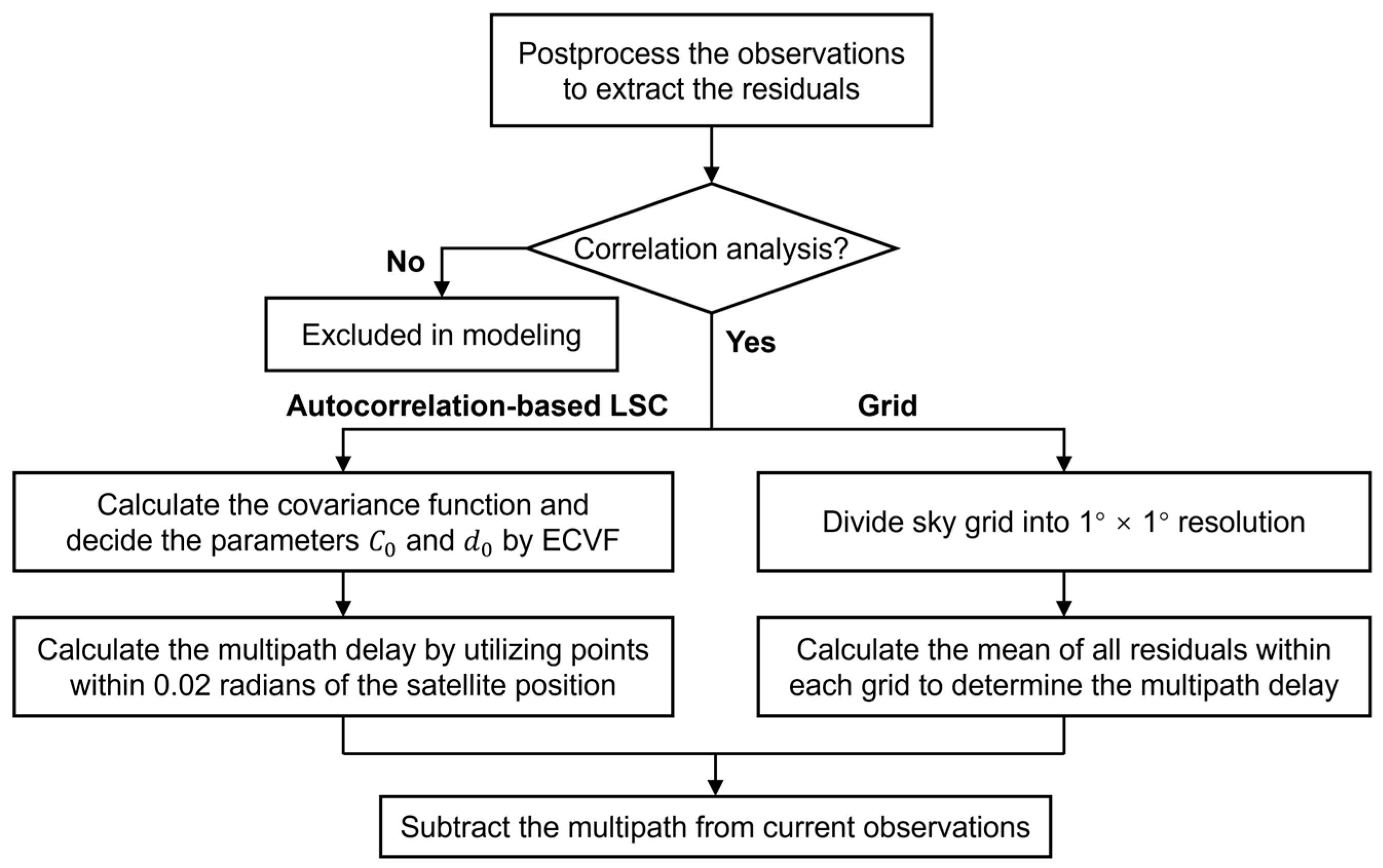
The spatial correlation characteristics of multipath are analyzed to enhance its mitigation in multi-GNSS, multi-frequency observations. This involves calculating the correlation coefficient between different GNSS frequencies, examining the spatial autocorrelation of residuals, and identifying consistent modeling parameters for the covariance function. Based on these findings, a spatial autocorrelation-based method utilizing a unified covariance function is proposed. Additionally, the impact of orbit shifts on long-term multipath error mitigation is evaluated, and strategies to reduce this impact are assessed. The flowchart of the procedure is plotted in Figure 2.

3. Computation and Analysis

3.1. Employed Data

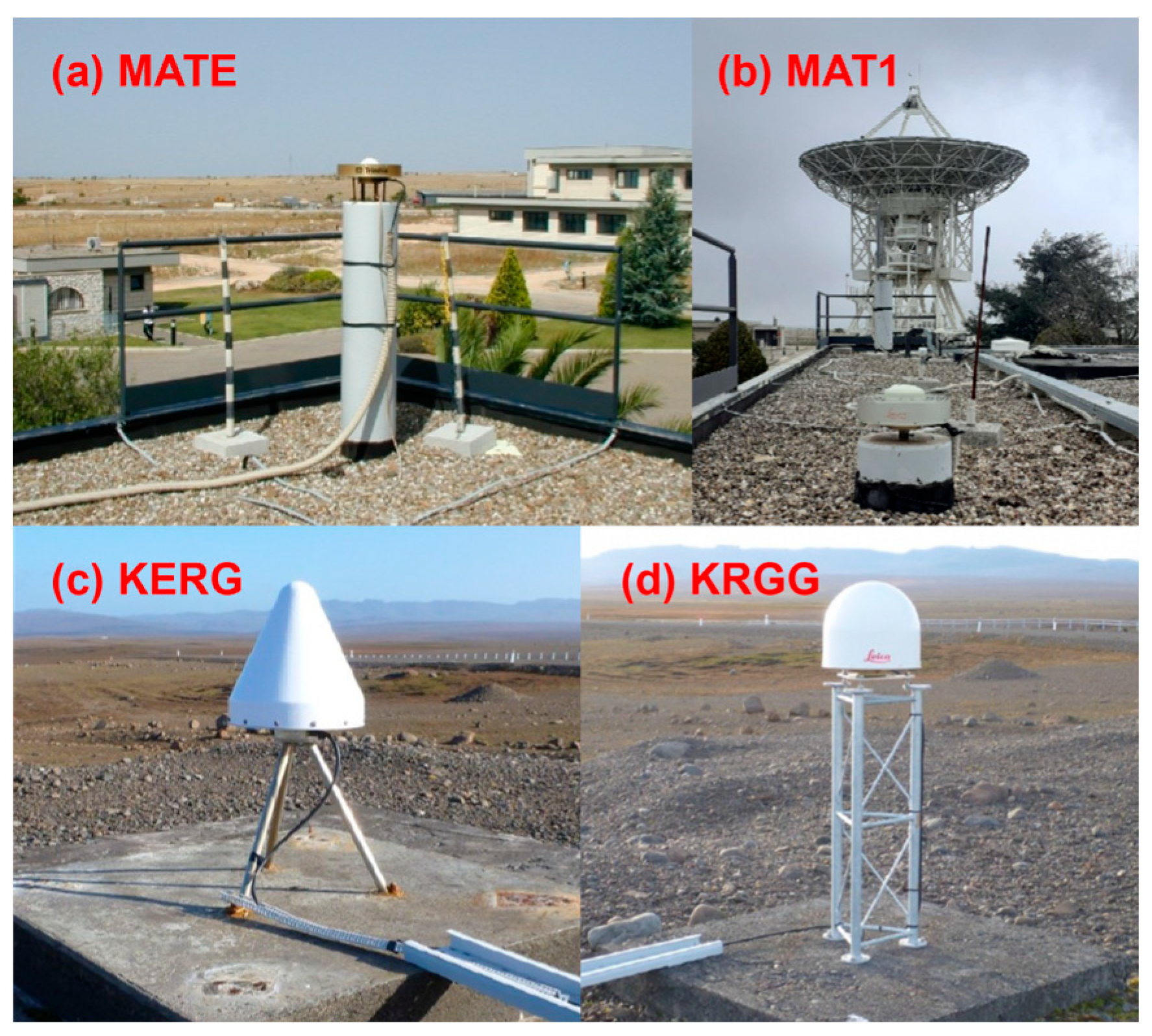
The observations from the short baselines MATE_MAT1 and KERG_KRGG, provided by the International GNSS Service, are utilized to analyze and validate methods for mitigating multipath effects. The lengths of these baselines are 10.7 m and 8.6 m, respectively, with a sampling interval of 30 s. The antenna photographs of the four stations are shown in Figure 3. Figure 4 illustrates the multipath distribution for both baselines, revealing that the errors are predominantly concentrated in low-elevation areas. The presence of a large metallic structure near station MAT1 leads to significant multipath errors in the MATE_MAT1 baseline, particularly around an elevation angle of 20° toward the southeast. Additionally, the KERG_KRGG baseline shows higher-frequency multipath errors in low-elevation regions, primarily due to the influence of ancillary equipment, such as antenna mounts [33].
Based on the satellite orbit repeat period of GPS and Galileo [13,34,35], we utilize 10 days of observation data from Days of the Year (DOY) 029–038 in 2023 for analysis and modeling, which are then applied to mitigate the multipath effects on DOY 039 and subsequent days. During this period, the GPS and Galileo frequencies available for each baseline are listed in Table 1, with specific frequency values. During data processing, a satellite elevation cutoff angle of 7° is applied, and the igs20_2309.atx antenna file is used to correct the phase center offsets (PCOs) and phase center variations (PCVs) for both satellites and receivers. For the KERG_KRGG baseline, due to the lack of Galileo PCO/PCV correction values, GPS PCO/PCV correction values are used as substitutes.

3.2. Correlation Analysis Between GPS/Galileo Frequencies

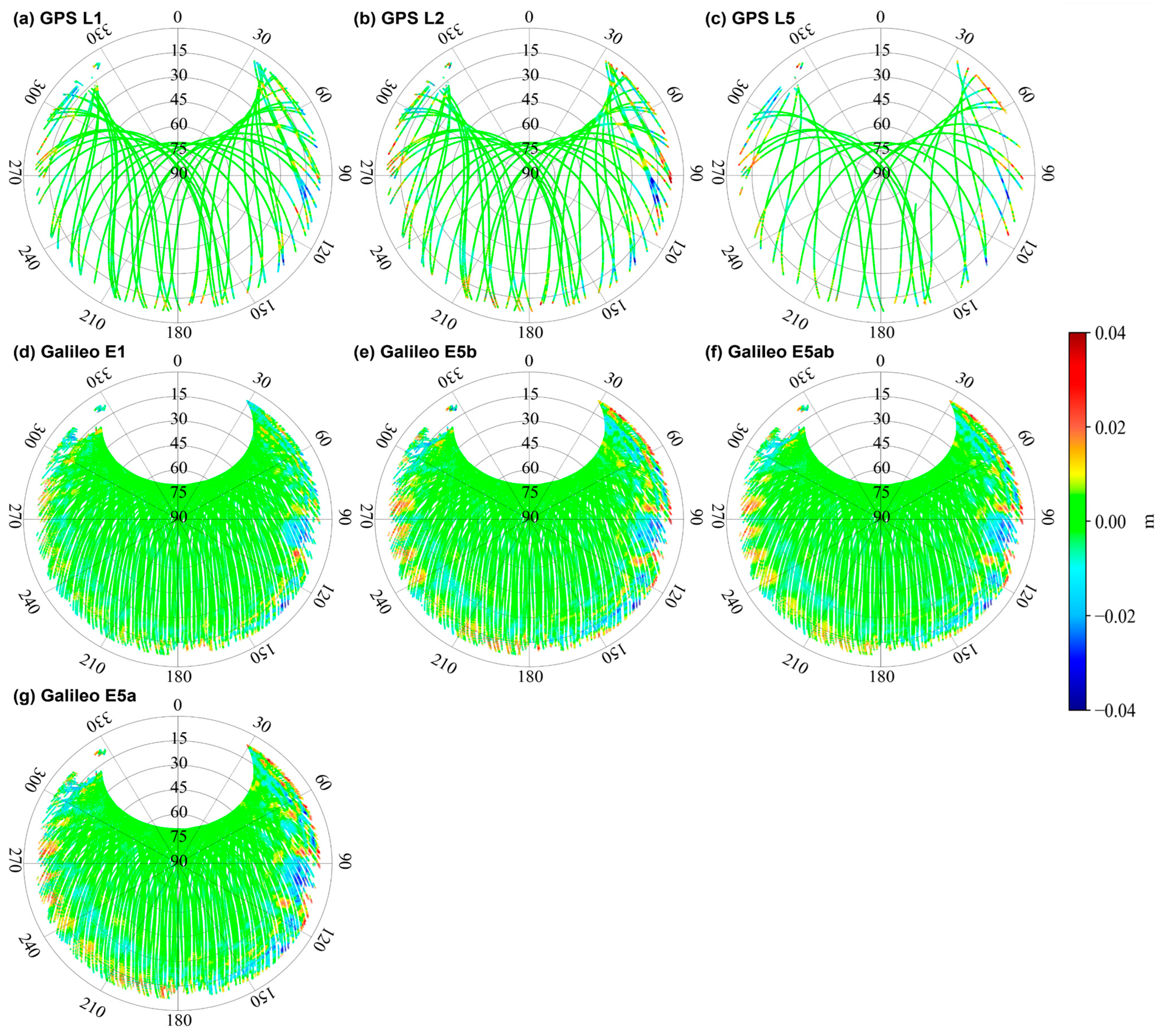
The carrier phase SD residual distribution for all frequencies of the MATE_MAT1 and KERG_KRGG baselines over the 10-day period from DOY 029–038 in 2023 is presented in Figure 5 and Figure 6. The SD residuals for satellites at low elevation angles (below 30°) are relatively large, a common feature associated with the heightened multipath effects in this region [36]. Additionally, it is noted that the number of satellites observed at the E5a frequency for the KERG_KRGG baseline is relatively low when the elevation angle is below 15°. This reduction is primarily due to the lack of low-elevation satellite data at the KERG station for this frequency.
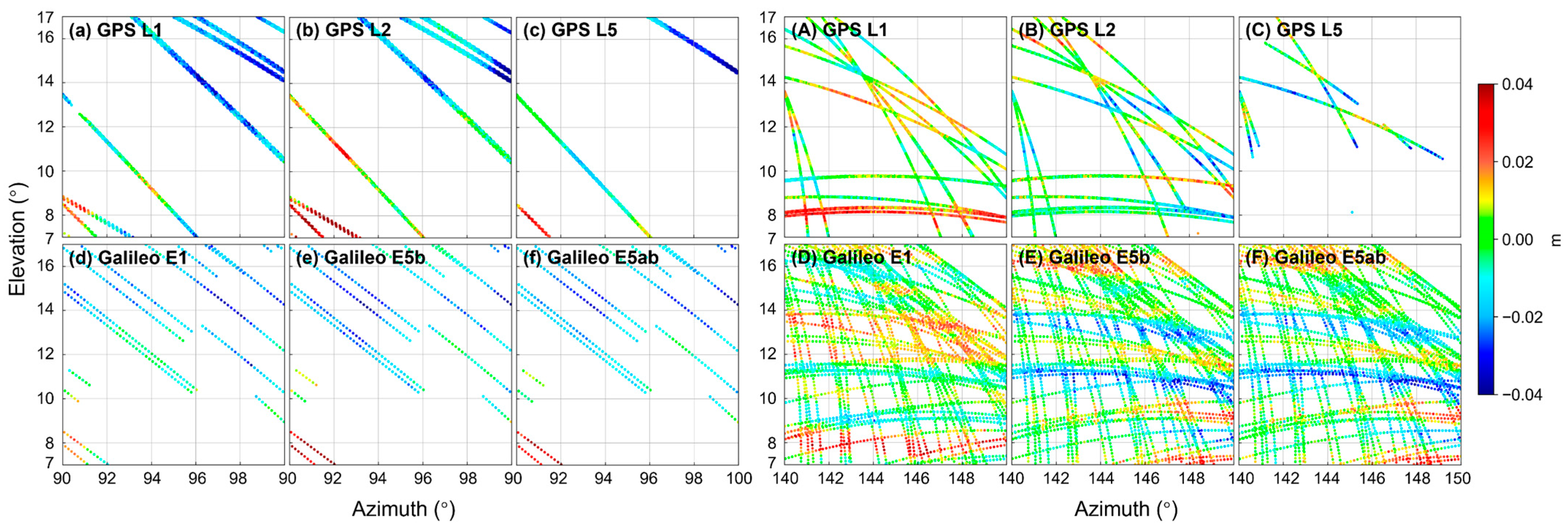
The residuals for the GPS L1/L2/L5 and Galileo E1/E5b/E5ab frequencies over a 10-day period, as the satellites traversed a designated square window, are presented in Figure 7, offering a comparative view of the signal variations across different GNSS frequencies. The windows for the MATE_MAT1 baseline cover an elevation angle of 7° to 17° and an azimuth angle of 90° to 100°, while for the KERG_KRGG baseline, the range is 7° to 17° in elevation and 140° to 150° in azimuth. A consistent pattern is observed for different frequencies at the same spatial locations. Notably, for overlapping or closely spaced frequencies, the satellite trajectory colors appear similar or nearly identical. For instance, this applies to overlapping frequencies such as GPS L1 and Galileo E1, closely spaced frequencies like GPS L2 and Galileo E5b, as well as GPS L5 and Galileo E5ab, all of which follow the same pattern. In contrast, for frequencies with larger differences, such as GPS L1 and Galileo E5b/E5ab, the trajectory colors vary significantly, and in some instances, even exhibit opposite sign values.
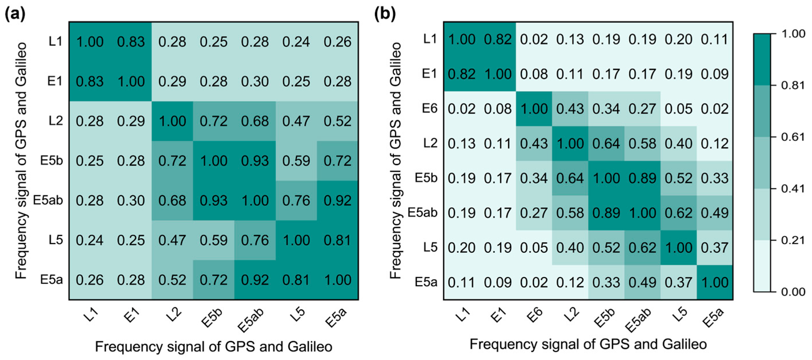
The Pearson correlation coefficient is used to evaluate the correlation between the residual sequences of any two frequencies. The absolute values of the resulting correlation coefficients are displayed in Figure 8, showing diagonal symmetry along the value of 1. To better visualize the strength of multipath error correlations between frequency pairs, a color gradient is applied, ranging from dark (strong correlation) to light (weak correlation). It is clear from the figure that correlations exist between multipath errors for all frequency pairs, though the strength of this correlation decreases as the frequency differences increase. Additionally, the relationship between frequency difference and the absolute value of the correlation coefficient is illustrated in Figure 9, offering a more intuitive visualization of how frequency differences affect correlation strength.
Due to the lack of low-elevation observations at the Galileo E5a frequency from the KERG station, the low correlations between E5a and the other frequencies in the KERG_KRGG baseline may not accurately reflect the true correlations. Apart from this, the residuals from frequency pairs, such as overlapping ones like L1/E1 and L5/E5a between GPS and Galileo, as well as non-overlapping frequencies like L2 and E5b, and the Galileo frequencies E5a, E5b, and E5ab, exhibit relatively large correlation coefficients, indicating strong correlations. Other frequencies also demonstrate strong to moderate correlations between narrow-spaced frequencies. These strong correlations suggest that their residuals contain similar multipath errors, supporting the potential for combining frequencies to enhance multipath error correction.

3.3. Parameters of Covariance Function

The covariance function used in this study is Markov’s function by Equation (11), where C 0 and d 0 determine the function. These parameters for different frequencies are initially calculated by fitting the theoretical function to the empirical covariance function and then compared across the frequencies.
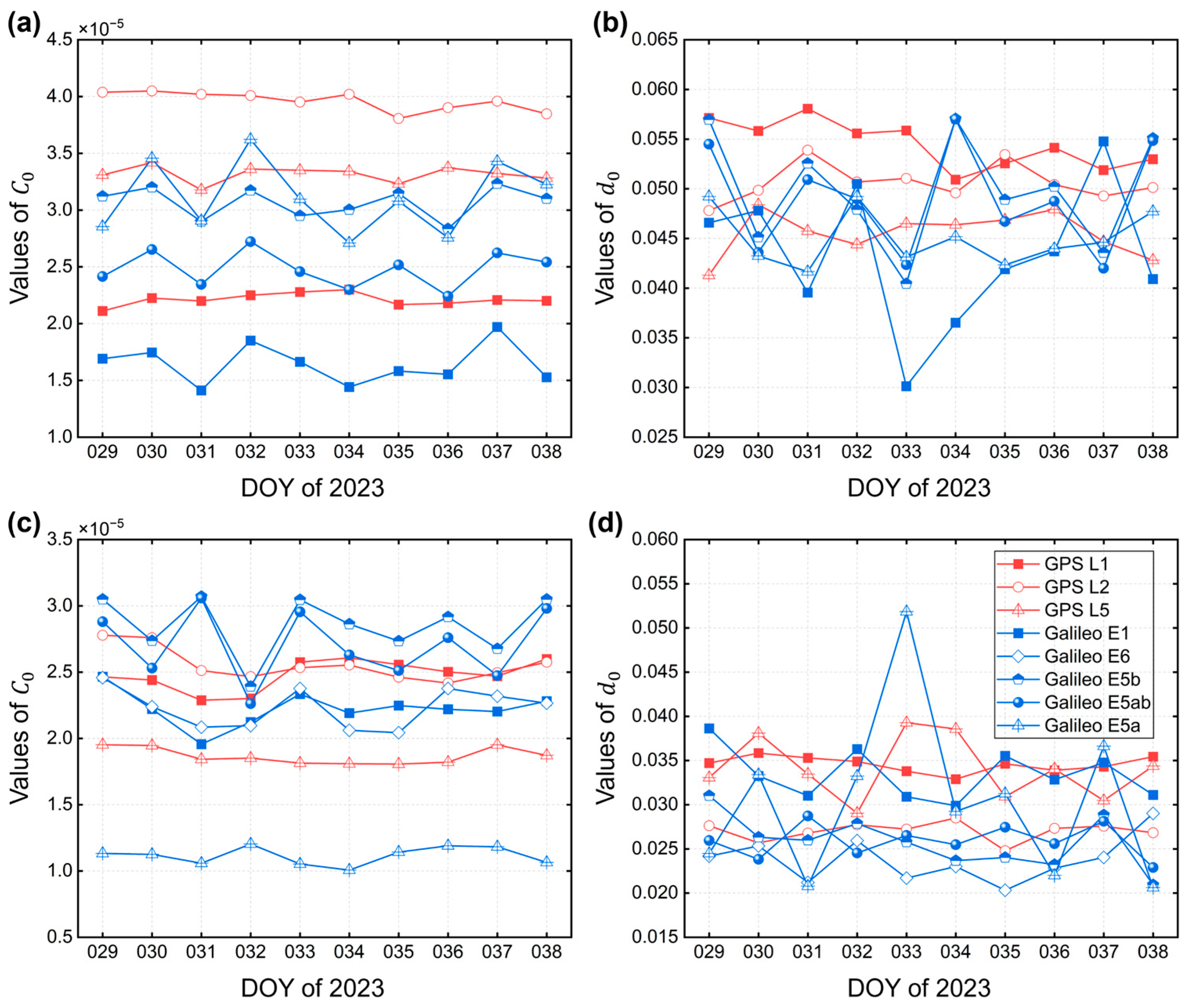
The computed and fitted ECVF curves for the GPS L1 and Galileo E1 frequencies, from the MATE_MAT1 and KERG_KRGG baselines on DOY 038 in 2023, are shown in Figure 10 as an example. The curves of other frequencies are similar to these two frequency signals. Figure 11 presents the computed values of C 0 and d 0 over a 10-day modeling period for both the GPS and Galileo frequencies for the two baselines.
The C 0 values for the MATE_MAT1 baseline are slightly larger than those for the KERG_KRGG baseline, though the ranges for both baselines overlap significantly. In contrast, the d 0 parameter for the MATE_MAT1 baseline is notably larger than for KERG_KRGG, which is expected due to the higher spatial frequency of multipath observed in the KERG_KRGG baseline.
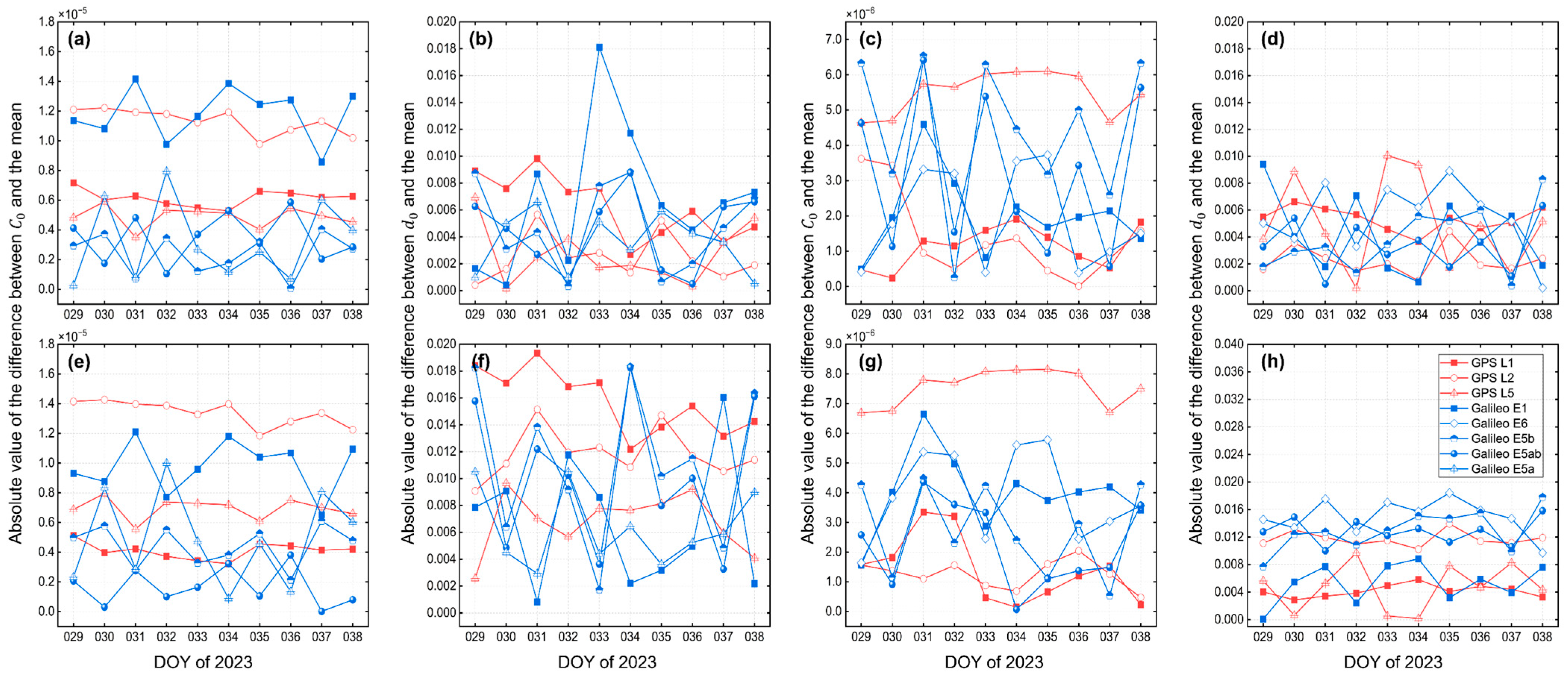
Additionally, the deviations of parameters relative to the averages of each single baseline and both baselines combined are computed and shown in Figure 12. Due to the absence of low-elevation data with large residuals at the E5a frequency for the KERG_KRGG baseline, the calculated covariance parameters are not representative of the multipath errors, leading to the exclusion of this frequency from the analysis. As anticipated, the differences between the original parameter values and the averages for each baseline are relatively small (Figure 12), while the deviations from the combined averages of both baselines are slightly larger. Nonetheless, the differences in C 0 for this case remain small, around 1 × 10⁻⁵, and the d 0 differences stay within 0.02.
The parameters C 0 and d 0 of all frequency residuals are unified by averaging all frequency parameters across two baselines. These unified parameters are then applied in a spatial autocorrelation-based method for multipath mitigation. To evaluate performance, GPS L1 frequency observations from both baselines are analyzed. The residual variance reduction rates after applying the unified parameters are displayed in Figure 13, alongside rates using average parameters for each baseline and for each frequency individually.
The results demonstrate that the variance reduction rates achieved with the unified parameters are comparable to those obtained with baseline-specific averages. This suggests that using unified covariance function parameters for different baselines and frequency signals is effective, simplifying the computational process by eliminating the need to estimate the parameters C 0 and d 0 individually. Moving forward, these unified parameters will be employed in subsequent research efforts.

3.4. Orbit Shift over a Long Time Span

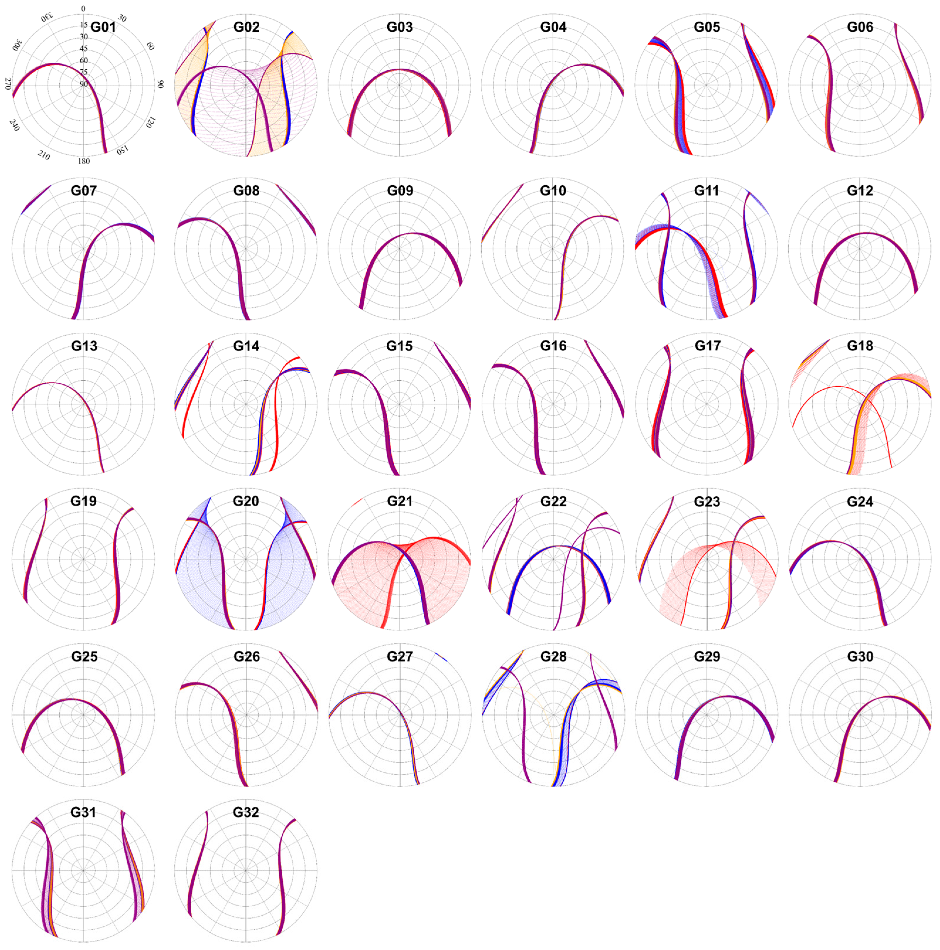
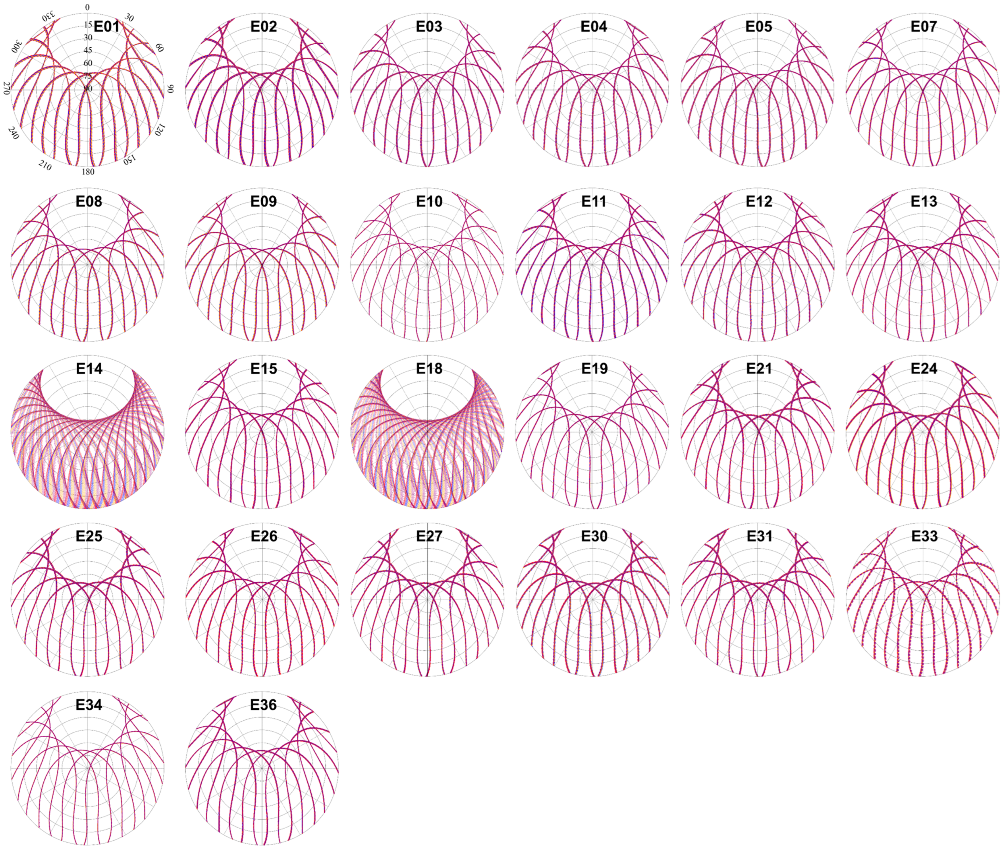
Due to various perturbations, satellite orbits exhibit drift, with variations across different satellites and systems. Figure 14 and Figure 15 depict the satellite tracks of all GPS and Galileo satellites observable at the MATE station over a four-year period, from 1 January 2020 to 31 December 2023. In these figures, the satellite tracks for 2020 are shown in red, 2021 in blue, 2022 in orange, and 2023 in purple, visually representing the orbit drift across the years.
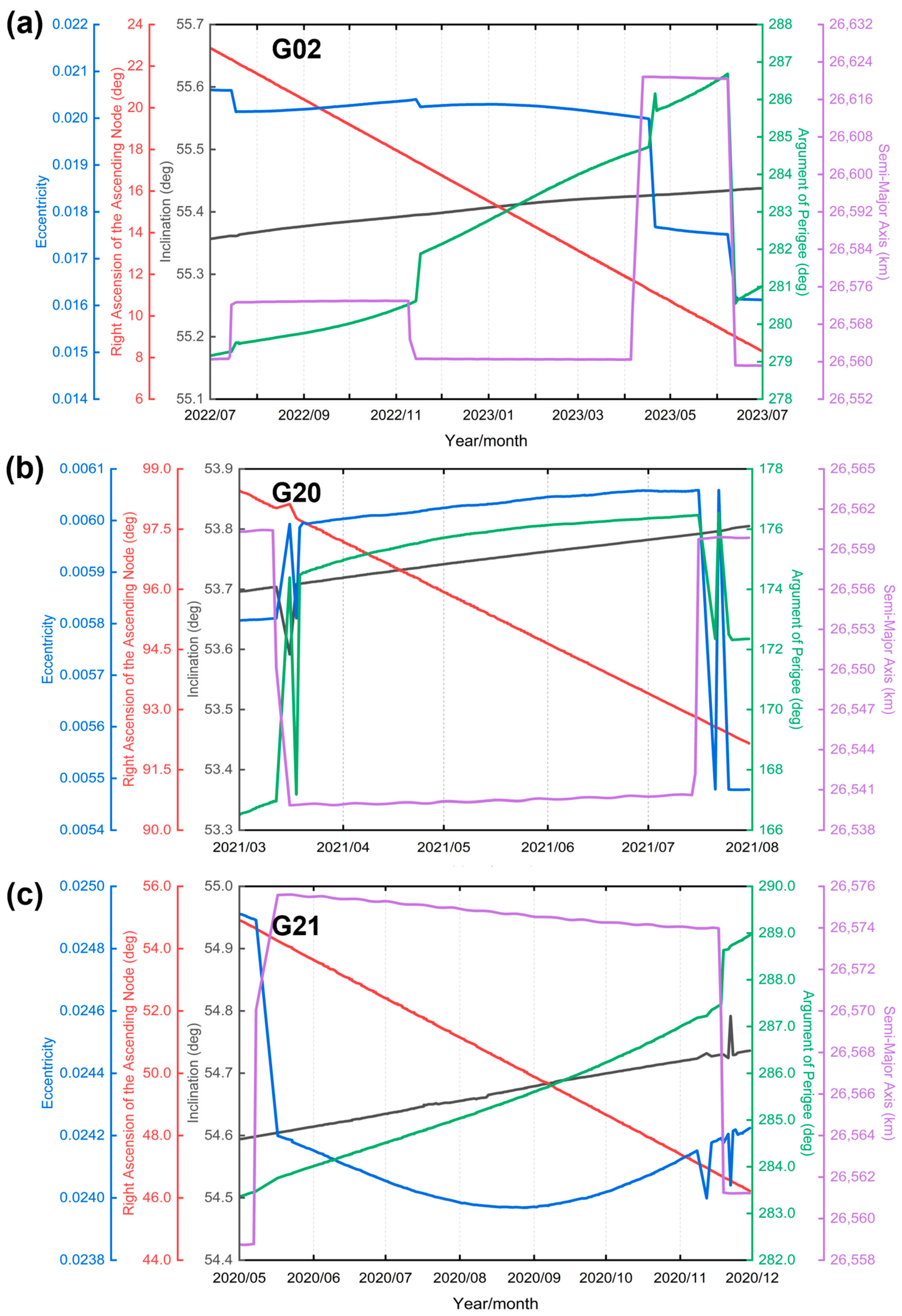
Within the Galileo system, satellites E14 and E18 show more pronounced orbit drift compared to others, indicating less stable orbits. Conversely, many GPS satellites exhibit significant orbit drift, notably satellite G02 in 2022 and 2023, G20 in 2021, and G21 in 2020, with their drift far exceeding that observed in the Galileo system. Specifically, substantial orbital drift was observed for G02 during July–November 2022 and April–June 2023, G20 during March–July 2021, and G21 during May–November 2020. Figure 16 illustrates the variation trends of selected orbital parameters—namely eccentricity, Right Ascension of the Ascending Node (RAAN), orbital inclination, argument of perigee, and semi-major axis—for these three satellites during the noted periods. Significant adjustments in these orbital parameters occurred during times of pronounced deviations in satellite trajectories. The significant changes in the semi-major axis correspond to a substantial variation in the satellite’s orbit repeat period. Consequently, if substantial changes occur in the orbital parameters such as the semi-major axis, the residual data from previous periods may not accurately represent the current multipath errors due to significant spatial discrepancies between the expected and actual satellite positions, leading to inaccuracies in multipath error correction.
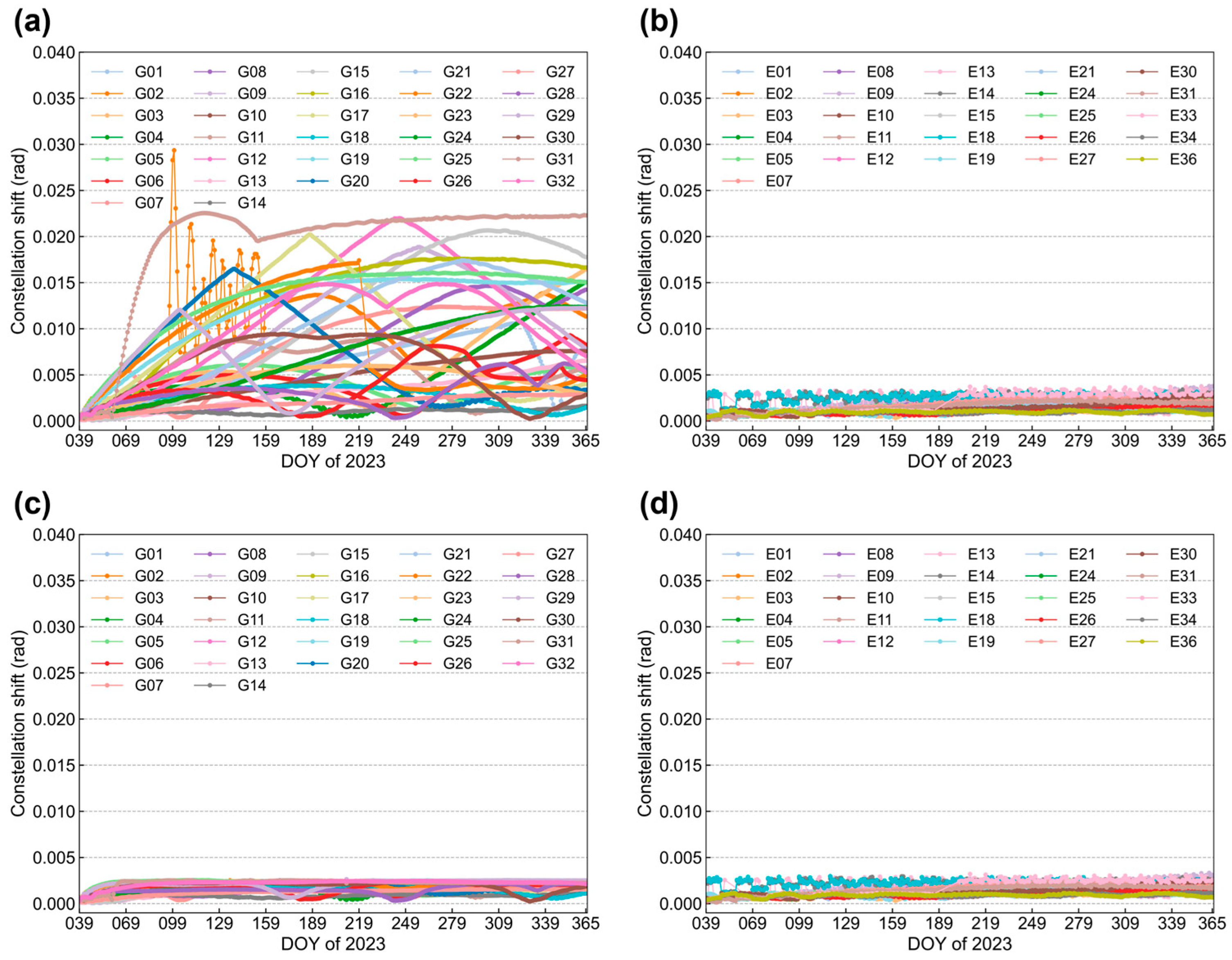
Utilizing orbital data from DOY 029–038 of 2023 as reference orbits for both the GPS and Galileo systems, the average unit spherical distance from the positions of satellites G01–G32 and E01–E36 during DOY 039–365 of 2023 to their nearest reference orbit was calculated. Figure 17a,b demonstrates these deviations. The average deviation distance for Galileo satellites remains relatively stable, peaking at only 0.004 rad, while that for GPS satellites shows a marked increase, with satellite G02 reaching a maximum deviation of 0.029 rad. Interestingly, around DOY 249, the average deviation for GPS satellites stabilizes.
By recalculating the average unit spherical distance using orbital data from DOY 239–248 as a new reference for the period DOY 249–365, the results, shown in Figure 18, reveal a reduction in the maximum average deviation for GPS satellites to 0.017 rad, which is significantly lower than earlier measurements. This adjustment indicates that using more recent data as reference orbits leads to more accurate multipath error correction, suggesting that outdated historical data may not effectively correct for current GPS multipath errors.
Based on the analysis in Section 3.2, there is a notable correlation in multipath errors between the GPS and Galileo systems, with overlapping or narrowly-spaced frequencies showing very strong correlation. Consequently, integrating these two systems could enhance the density of orbit trajectories, potentially mitigating the negative impacts of GPS orbit shifts on long-term multipath correction.
Using orbital data from both GPS and Galileo systems from DOY 029–038 of 2023, a combined reference orbit was established. We calculated the average unit spherical distance from the positions of satellites G01–G32 and E01–E36 to this combined orbit for the same period. The results, shown in Figure 17c,d, reveal that while the average deviation distance for Galileo satellites from the combined orbit remains stable at 0.004 rad, the deviation for GPS satellites shows a significant reduction to 0.003 rad. Additionally, these distances do not exhibit significant long-term fluctuations.
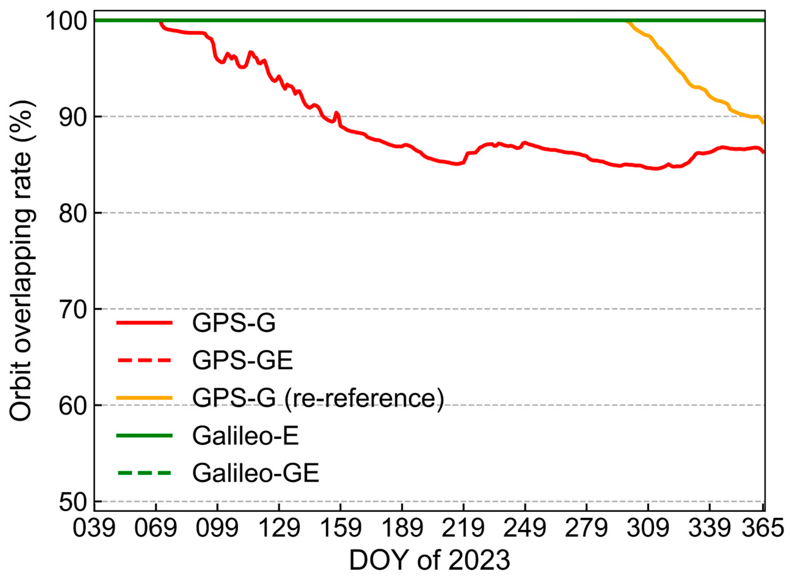
In Figure 17, the average deviation distances for both GPS and Galileo satellite orbits generally stay within 0.02 rad. Using this threshold, satellite coordinates within this distance from the reference orbit on a unit sphere are considered consistent, indicating an orbit repeat. Orbit repeatability for both systems is then calculated daily from DOY 039 to 365 in 2023 and is presented in Figure 19, with reference to both individual constellations and the combined constellation. When using the GPS satellite orbits from DOY 239 to 248 as the reference, the GPS orbit repeatability gradually declines, dropping to 84.5% after DOY 072. This reduction negatively impacts the accuracy and stability of the multipath error model. However, when GPS and Galileo satellite orbits are combined, the GPS orbit repeatability remains stable at 100%. Galileo satellites consistently show 100% repeatability throughout the observation period, thanks to their inherent orbital stability. Thus, integrating GPS and Galileo systems for multipath modeling and mitigation is expected to improve correction accuracy and ensure more stable results, particularly for GPS.

3.5. Unified Covariance Function Parameters for Short and Long-Term Multipath Correction Analysis

Using the MATE_MAT1 baseline’s GPS L1 and Galileo E1 frequencies as examples, we applied both the grid method and the autocorrelation-based LSC using unified covariance function parameters in the multipath mitigation. The calibration, carried out from DOY 039 to 365 in 2023, employs a 30-day interval. The moving neighborhood parameter is set at 0.02 rad, and the covariance function parameters C 0 and d 0 are averaged across all frequencies from both baselines. The specific strategies for multipath correction are detailed in Table 2.
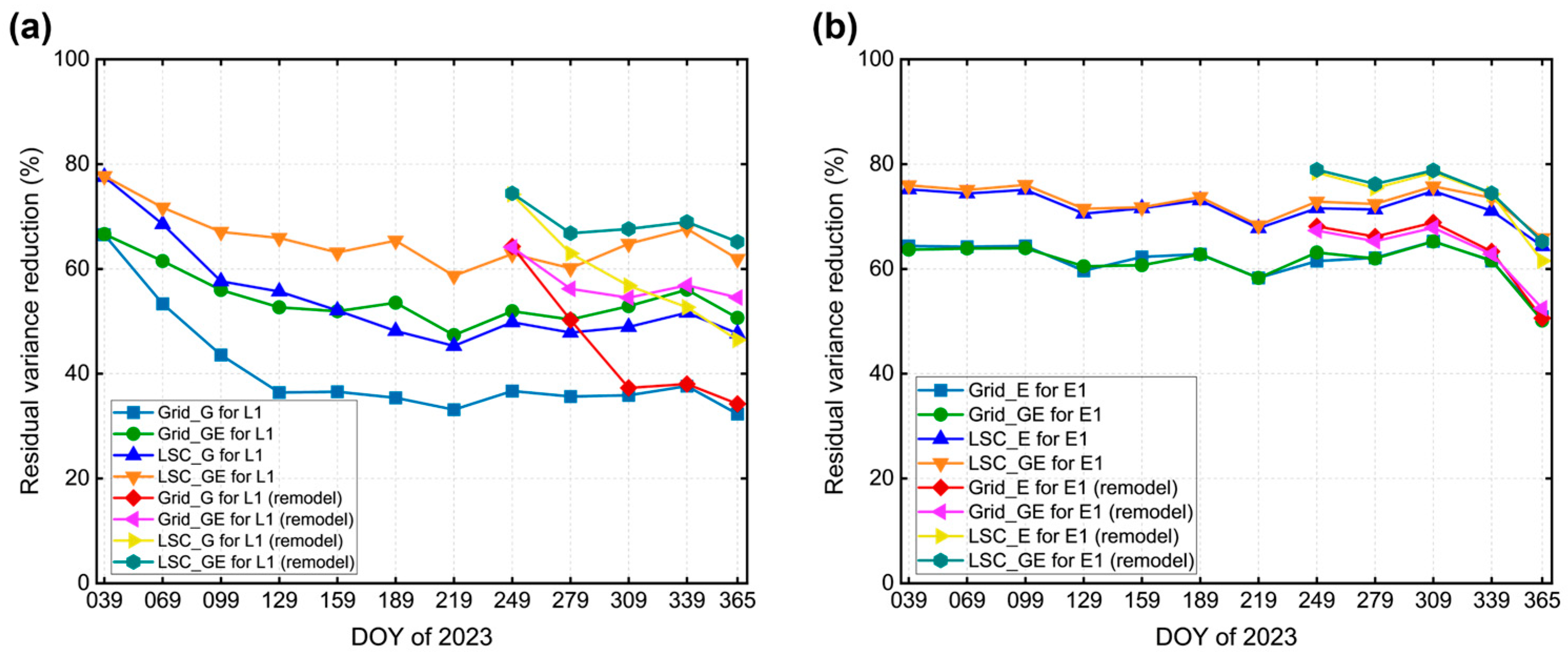
The standard deviations of the SD residuals before and after applying the multipath correction strategies are detailed in Table 3 and Table 4. On DOY 039 of 2023, the performance of the grid methods, labeled Grid_G and Grid_GE, are initially comparable. However, Grid_G’s performance declines more rapidly over time. In contrast, the LSC method demonstrates robust initial performance, maintaining superiority over Grid_G and showing slightly lesser performance only compared to the combined GPS/Galileo grid method after 120 days. The LSC_GE strategy, specifically modeled on DOY 029–038, consistently offers superior performance compared to all other strategies modeled on later dates (DOY 239–248).
Regarding the Galileo E1 frequency, the combined GPS/Galileo correction strategy proves to be as effective or slightly more so than the Galileo-only approach. This effectiveness persists even after 210 days of modeling, where the LSC_GE strategy consistently surpasses the grid method’s performance. This trend is maintained irrespective of whether the correction strategy involves only Galileo or a GPS/Galileo combination, with the combined LSC method achieving the best results. Thus, the study confirms the advantage of employing unified covariance function parameters for diverse baselines and frequency signals, which simplifies the computational process and enhances the effectiveness of multipath error mitigation.
Then, the residual variance reduction rate calculated by 1 σ 1 2 / σ 0 2 × 100 % , where σ 1 2 is the remaining SD residual variance after multipath correction and σ 0 2 denotes the uncorrected SD residual variance, is shown in Figure 20. For GPS L1, the variance reduction rate on DOY 039 of 2023 using the LSC_GE strategy shows improvements of 0.13%, 11.05%, and 11.16% over LSC_G, Grid_GE, and Grid_G, respectively. By DOY 365 of 2023, these improvements markedly increase to 14.24%, 11.25%, and 29.59%, respectively. This suggests that the LSC_GE strategy not only enhances multipath correction immediately after model application but maintains superior correction capabilities over extended periods. Additionally, the LSC_GE’s variance reduction consistently exceeds that achieved by the other strategies, even following repeated modeling. For the Galileo E1 frequency, the LSC_GE strategy improves the variance reduction rate by 0.75%, 12.27%, and 11.58% over LSC_E, Grid_GE, and Grid_E respectively on the first day. By DOY 365, these improvements rise to 1.5%, 15.69%, and 14.96%, respectively. Notably, the grid method’s performance post-re-modeling remains inferior to the pre-re-modeling performance of the LSC method. On DOY 339, the re-modeled LSC_E strategy matches the pre-re-modeling performance of the LSC_GE strategy, but it falls short after this period. The re-modeled LSC_GE strategy maintains similar performance to the pre-re-modeling performance of the LSC_GE.
Kinematic mode processing of GPS L1 and Galileo E1 data was conducted using the outlined strategies, with the results presented in Figure 21. The LAMBDA method was employed for ambiguity estimation in the processing, and the ambiguity fixing rates were over 99%. This figure displays the root mean square (RMS) values for the North, East, and Up components before and after multipath calibration. The combined GPS/Galileo solution for GPS L1 provided better results than the GPS-only solution. For Galileo E1, the combined solution was on par with the Galileo-only solution. Across both frequencies, the autocorrelation-based LSC using unified covariance function parameters yielded lower RMS errors and enhanced positioning accuracy compared to the grid method, indicating its efficacy whether applied to combined or single-system data.

4. Results

Multipath error significantly affects the accuracy of GNSS precise positioning but can be effectively mitigated using spatial autocorrelation-based methods in static and quasi-static environments. Traditional techniques like sidereal filtering and grid-based approaches only approximate the handling of spatial autocorrelation data. However, the spatiotemporal correlations of multipath can be more accurately modeled by utilizing the covariance function. This study investigates the spatial cross-correlation between different frequency bands across various GNSS systems, along with spatial autocorrelation function parameters and the effects of constellation shifts, to simplify autocorrelation-based methods like Least-Squares Collocation and enhance long-term performance.
The results reveal that overlapping frequencies, such as L1/E1 and L5/E5a, show very strong correlations, while non-overlapping frequencies, such as L2 and E5b, also exhibit strong correlations, with coefficients exceeding 0.8. The covariance function parameters, typically including the residual variance and the range parameter that control the rate of correlation decay with distance, remain relatively consistent across frequencies. This consistency allows autocorrelation-based methods using unified covariance function parameters to achieve a variance reduction rate (VRR) comparable to methods that rely on frequency-specific covariance function parameters. Additionally, the GPS satellites G02, G20, and G21 exhibit noticeable orbit shifts, leading to significant changes in orbital parameters and satellite tracks, which diminishes the effectiveness of long-term multipath mitigation. These satellites display larger average deviations, reaching a maximum deviation of 0.029 rad. In contrast, the Galileo satellites demonstrate more stable orbits, with fluctuations confined to 0.004 rad. When combining GPS and Galileo reference orbits, the maximum deviation for GPS satellites reduces to 0.003 rad, and the orbital repeat rate stabilizes at 100%.
Multipath mitigation experiments using both the grid method and the autocorrelation-based LSC with a unified covariance function for GPS L1 and Galileo E1 frequencies on the MATE_MAT1 baseline were conducted. This analysis considers the GPS, Galileo, and combined GPS/Galileo data separately. For GPS L1, the LSC_GE strategy improves the residual variance reduction rate by 0.13%, 11.05%, and 11.16% compared to LSC_G, Grid_GE, and Grid_G, respectively, on DOY 039, the first day after modeling. These improvements increase to 14.24%, 11.25%, and 29.59% on DOY 365, 327 days from the modeling data. Similarly, for Galileo E1, the LSC_GE strategy shows improvements of 0.75%, 12.27%, and 11.58% on the first day following modeling, rising to 1.5%, 15.69%, and 14.96% by DOY 365. As a result, the accuracy of kinematic positioning is improved.
Overall, the unified covariance function proves effective for autocorrelation-based multipath mitigation, outperforming conventional grid methods. Although GPS orbit drift negatively affects long-term mitigation, integrating GPS and Galileo data consistently produces lower RMS values and more accurate baseline solutions, significantly mitigating the impact of orbit drift. However, the method is based on spatial autocorrelation. Therefore, in the case that the spatial autocorrelation is low, the performance will be limited. This may happen in complex multipath environments. However, this need to be tested when complex multipath environments are encountered in practice.

Author Contributions

Conceptualization, W.X. and Y.T.; methodology, W.X. and Y.T.; software, W.X. and Y.T.; validation, X.D. and Q.Z.; formal analysis, Y.L. and X.D.; investigation, X.R.; writing—original draft preparation, W.X.; writing—review and editing, Y.T. and Q.Z.; visualization, Y.L. and X.R.; supervision, Y.T. All authors have read and agreed to the published version of the manuscript.

Funding

This research was funded by the National Natural Science Foundation of China, grant number 42274032.

Data Availability Statement

The GNSS raw observation data are available at http://www.igs.org/mgex/data-products/#data (accessed on 12 March 2024).

Conflicts of Interest

The authors declare no conflicts of interest.

References

  1. Groves, P.D.; Jiang, Z. Height Aiding, Weighting and Consistency Checking for GNSS NLOS and Multipath Mitigation in Urban Areas. J. Navig. 2013, 66, 653–669. [Google Scholar] [CrossRef]
  2. Manandhar, D.; Shibasaki, R.; Torimoto, H. GPS Reflected Signal Analysis using Software Receiver. J. Glob. Position. Syst. 2006, 5, 29–34. [Google Scholar] [CrossRef]
  3. Tranquilla, J.M.; Carr, J.P.; Alrizzo, H.M. Analysis of a choke ring groundplane for multipath control in global positioning system (gps) applications. IEEE Trans. Antennas Propag. 1994, 42, 905–911. [Google Scholar] [CrossRef]
  4. Tatarnikov, D.V.; Stepanenko, A.P.; Astakhov, A.V. Moderately compact helix antennas with cutoff patterns for millimeter RTK positioning. Gps Solut. 2016, 20, 587–594. [Google Scholar] [CrossRef]
  5. Vandierendonck, A.J.; Fenton, P.; Ford, T.; Inst, N. Theory and performance of narrow correlator spacing in a gps receiver. In Proceedings of the National Technical Meeting of the Inst of Navigation, San Diego, CA, USA, 27–29 January 1992; pp. 115–124. [Google Scholar]
  6. Axelrad, P.; Comp, C.J.; MacDoran, P.F. SNR-based multipath error correction for GPS differential phase. IEEE Trans. Aerosp. Electron. Syst. 1996, 32, 650–660. [Google Scholar] [CrossRef]
  7. Bilich, A.; Larson, K.M. Mapping the GPS multipath environment using the signal-to-noise ratio (SNR). Radio Sci. 2008, 43, RS6003. [Google Scholar] [CrossRef]
  8. Zhang, Z.T.; Li, B.F.; Gao, Y.; Shen, Y.Z. Real-time carrier phase multipath detection based on dual-frequency C/N0 data. Gps Solut. 2019, 23, 7. [Google Scholar] [CrossRef]
  9. Zheng, D.W.; Zhong, P.; Ding, X.L.; Chen, W. Filtering GPS time-series using a Vondrak filter and cross-validation. J. Geod. 2005, 79, 363–369. [Google Scholar] [CrossRef]
  10. Satirapod, C.; Rizos, C. Multipath mitigation by wavelet analysis for GPS base station applications. Surv. Rev. 2005, 38, 2–10. [Google Scholar] [CrossRef]
  11. Zhong, P.; Ding, X.L.; Zheng, D.W.; Chen, W.; Huang, D.F. Adaptive wavelet transform based on cross-validation method and its application to GPS multipath mitigation. Gps Solut. 2008, 12, 109–117. [Google Scholar] [CrossRef]
  12. Bernelli-Zazzera, F.; Campana, R.; Gottifredi, F.; Marradi, L. GPS attitude determination by Kalman filtering: Simulation of multipath rejection. In Proceedings of the 8th Annual Space Flight Mechanics Meeting, Monterey, CA, USA, 9–11 February 1998; pp. 1391–1405. [Google Scholar]
  13. Agnew, D.C.; Larson, K.M. Finding the repeat times of the GPS constellation. Gps Solut. 2007, 11, 71–76. [Google Scholar] [CrossRef]
  14. Genrich, J.F.; Bock, Y. Rapid resolution of crustal motion at short ranges with the global positioning system. J. Geophys. Res. Solid. Earth 1992, 97, 3261–3269. [Google Scholar] [CrossRef]
  15. Zhong, P.; Ding, X.L.; Yuan, L.G.; Xu, Y.L.; Kwok, K.; Chen, Y.Q. Sidereal filtering based on single differences for mitigating GPS multipath effects on short baselines. J. Geod. 2010, 84, 145–158. [Google Scholar] [CrossRef]
  16. Cohen, C.E.; Parkinson, B.W. Mitigating multipath error in gps based attitude determination. In Proceedings of the 14th Annual Rocky Mountain Conf on Guidance and Control, Keystone, CO, USA, 2–6 February 1991; pp. 53–68. [Google Scholar]
  17. Dong, D.; Wang, M.; Chen, W.; Zeng, Z.; Song, L.; Zhang, Q.; Cai, M.; Cheng, Y.; Lv, J. Mitigation of multipath effect in GNSS short baseline positioning by the multipath hemispherical map. J. Geod. 2016, 90, 255–262. [Google Scholar] [CrossRef]
  18. Fuhrmann, T.; Luo, X.G.; Knöpfler, A.; Mayer, M. Generating statistically robust multipath stacking maps using congruent cells. Gps Solut. 2015, 19, 83–92. [Google Scholar] [CrossRef]
  19. Wang, Z.R.; Chen, W.; Dong, D.N.; Wang, M.H.; Cai, M.M.; Yu, C.; Zheng, Z.Q.; Liu, M. Multipath mitigation based on trend surface analysis applied to dual-antenna receiver with common clock. Gps Solut. 2019, 23, 104. [Google Scholar] [CrossRef]
  20. Zheng, K.; Zhang, X.H.; Li, P.; Li, X.X.; Ge, M.R.; Guo, F.; Sang, J.Z.; Schuh, H. Multipath extraction and mitigation for high-rate multi-GNSS precise point positioning. J. Geod. 2019, 93, 2037–2051. [Google Scholar] [CrossRef]
  21. Hofmann-Wellenhof, B.; Moritz, H. Physical Geodesy; Springer: Vienna, Austria, 2005. [Google Scholar]
  22. Lin, M. Regional Gravity Field Recovery Using The Point Mass Method. Ph.D. Thesis, Leibniz Universität Hannover, Hannover, Germany, 2016. [Google Scholar]
  23. Moritz, H. Advanced Physical Geodesy; Wichmann: Berlin, Germany, 1980. [Google Scholar]
  24. Tian, Y.; Liu, Z.; Lin, M.; Li, K. Modelling and mitigation of GNSS multipath effects by least-squares collocation considering spatial autocorrelation. J. Geod. 2023, 97, 37. [Google Scholar] [CrossRef]
  25. Lu, R.; Chen, W.; Li, Z.; Dong, D.A.; Jiang, W.P.; Wang, Z.R.; Huang, L.Y.; Duan, X.L. An improved joint modeling method for multipath mitigation of GPS, BDS-3, and Galileo overlapping frequency signals in typical environments. J. Geod. 2023, 97, 95. [Google Scholar] [CrossRef]
  26. Geng, J.H.; Li, P.B.; Li, G.C. Combining the GPS/Galileo/BDS-3 signals on overlap frequencies for interoperable multipath hemispherical maps. J. Geod. 2024, 98, 32. [Google Scholar] [CrossRef]
  27. Krag, H.; Leonard, A.; Ranaudo, P.; Blomenhofer, E. Global Implications of GPS and Galileo RAAN Drifts on GNSS Performance. In Proceedings of the 16th International Technical Meeting of the Satellite Division of The Institute of Navigation (ION GPS/GNSS 2003), Portland, OR, USA, 9–12 September 2003. [Google Scholar]
  28. Pellegrino, M.M.; Scheeres, D.J.; Streetman, B.J. The Feasibility of Targeting Chaotic Regions in the GNSS Regime. J. Astronaut. Sci. 2021, 68, 553–584. [Google Scholar] [CrossRef]
  29. Sosnica, K.; Bury, G.; Zajdel, R.; Ventura-Traveset, J.; Mendes, L. GPS, GLONASS, and Galileo orbit geometry variations caused by general relativity focusing on Galileo in eccentric orbits. Gps Solut. 2022, 26, 5. [Google Scholar] [CrossRef]
  30. Moritz, H. Covariance Functions in Least-Squares Collocation; Ohio State University Research Foundation: Columbus, OH, USA, 1976; Volume 240. [Google Scholar]
  31. Moritz, H. Advanced Least-Squares Methods; Ohio State University Research Foundation: Columbus, OH, USA, 1972; Volume 175. [Google Scholar]
  32. Pearson, W.H. Estimation of a correlation coefficient from an uncertainty measure. Psychometrika 1966, 31, 421–433. [Google Scholar] [CrossRef] [PubMed]
  33. Liu, Z.F.; Tian, Y.M.; Xiong, W.H.; Liang, Y.B.; Li, K.G.; Tan, S.H.; Yang, X.W.; Li, N. A local filtering approach to mitigating the GNSS multipath effects in relative precise positioning considering the multipath spatial correlation. Adv. Space Res. 2024, 74, 2709–2727. [Google Scholar] [CrossRef]
  34. Ragheb, A.E.; Clarke, P.J.; Edwards, S.J. GPS sidereal filtering: Coordinate- and carrier-phase-level strategies. J. Geod. 2007, 81, 325–335. [Google Scholar] [CrossRef]
  35. Wang, M.; Wang, J.; Dong, D.; Li, H.; Han, L.; Chen, W. Comparison of Three Methods for Estimating GPS Multipath Repeat Time. Remote Sens. 2018, 10, 6. [Google Scholar] [CrossRef]
  36. Larson, K.M.; Bilich, A.; Axelrad, P. Improving the precision of high-rate GPS. J. Geophys. Res.-Solid. Earth 2007, 112, B05422. [Google Scholar] [CrossRef]
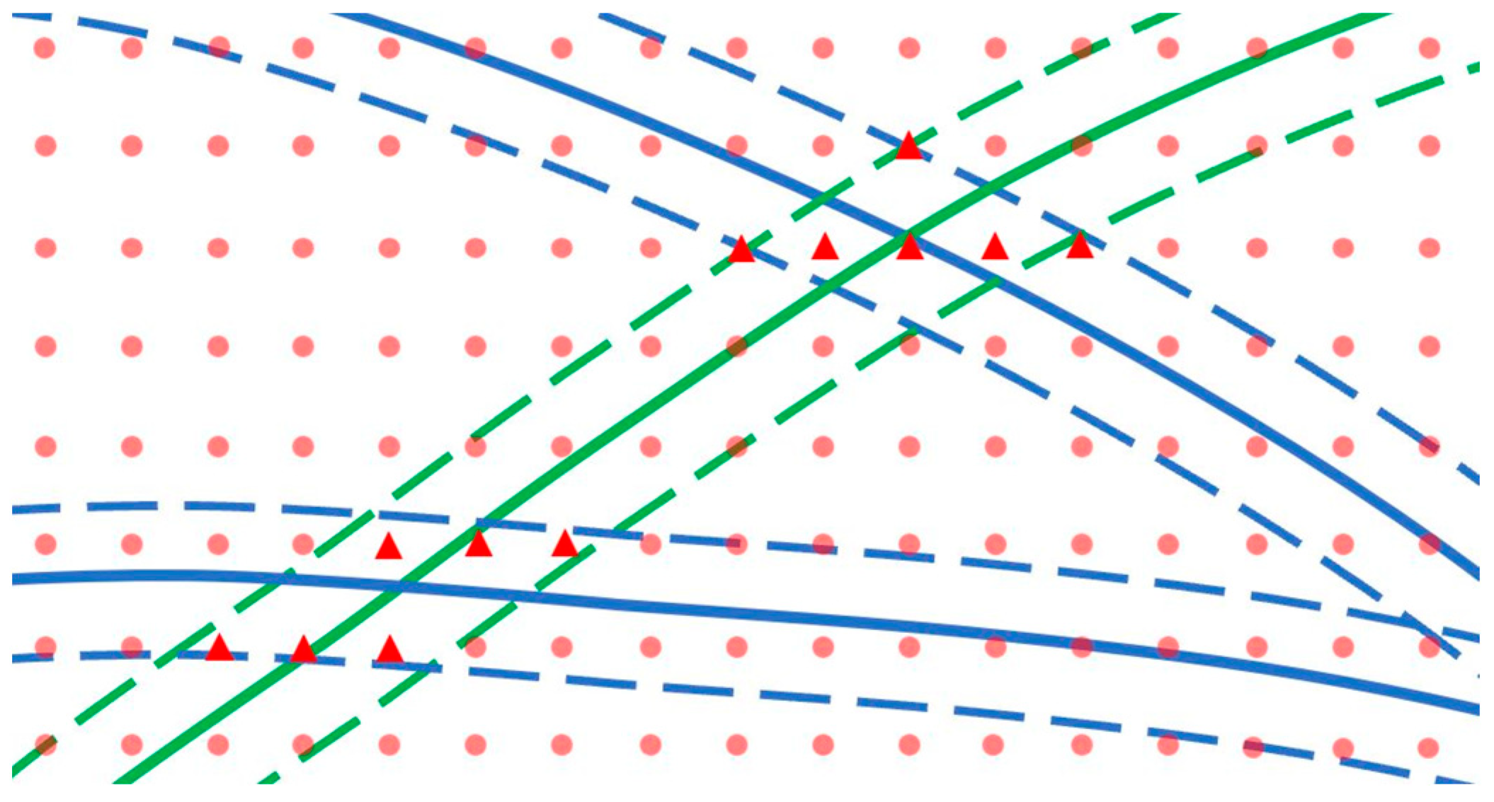
Figure 1. Schematic diagram of the data locations used to calculate the correlation between residuals from different frequencies. The blue and green solid lines represent satellite tracks from two distinct systems, while the blue and green dashed lines indicate the 0.02 radians boundaries to the satellite tracks. All red points, including the red circles and red triangles, represent uniformly distributed samples generated for the correlation analysis. The red triangles are the points that fall within the 0.02 radians overlapping region around the satellite tracks of both systems, i.e., the region where the dashed lines overlap. The red circles represent points that fall outside the overlapping region and are therefore excluded from the analysis.
Remotesensing 16 04009 g001
Figure 2. Flowchart of multipath analysis and mitigation.
Remotesensing 16 04009 g002
Figure 3. Antenna photographs of MATE_MAT1 (a,b) and KERG_KRGG (c,d). Photographs are from www.sonel.org (accessed on 14 October 2024).
Remotesensing 16 04009 g003
Figure 4. Multipath distributions for the baselines MATE_MAT1 (a) and KERG_KRGG (b). The red boxed area in (a) represents the significant multipath errors of the MATE_MAT1 baseline around an elevation angle of 20° toward the southeast.
Remotesensing 16 04009 g004
Figure 5. Satellite tracks and SD residuals for all frequencies of the baseline MATE_MAT1 on DOY 029–038 of 2023.
Remotesensing 16 04009 g005
Figure 6. Satellite tracks and SD residuals for all frequencies of the baseline KERG_KRGG on DOY 029–038 of 2023.
Remotesensing 16 04009 g006
Figure 7. SD residuals for different frequencies of the MATE_MAT1 baseline ((af), 7°–17° in elevation and 90°–100° in azimuth) and the KERG_KRGG baseline ((AF), 7°–17° in elevation and 140°–150° in azimuth).
Remotesensing 16 04009 g007
Figure 8. Absolute values of correlation coefficients between all frequencies of the baselines MATE_MAT1 (a) and KERG_KRGG (b). Utilizing a color gradient ranging from dark to light to represent the hierarchical levels of correlation strength, spanning from very strong to very weak or no correlation.
Remotesensing 16 04009 g008
Figure 9. Variation of all correlation coefficients with frequency differences for the baselines MATE_MAT1 (a) and KERG_KRGG (b).
Remotesensing 16 04009 g009
Figure 10. Theoretical covariance functions and ECVFs of GPS L1 and Galileo E1 for MATE_MAT1 (a,b) and KERG_KRGG (c,d) on DOY 038 of 2023. The blue dot curve is the ECVF derived with the GPS L1 (a,c) and Galileo E1 (b,d) SD residuals. The red curve is the fitted curve.
Remotesensing 16 04009 g010
Figure 11. Daily C 0 and d 0 parameters for MATE_MAT1 (a,b) and KERG_KRGG (c,d) on DOY 028–039 of 2023.
Remotesensing 16 04009 g011
Figure 12. Deviations of the parameters respective to the average of each single baseline (ad) and both baselines (ef) are computed, separately, for MATE_MAT1 (a,b,e,f) and KERG_KRGG (c,d,g,h).
Remotesensing 16 04009 g012
Figure 13. Variance reduction rates of SD residuals after multipath correction using different parameter values. The results of the parameters C 0 and d 0 by averaging all frequency parameters across two baselines (mean of the two baselines), averaging parameters for each baseline (mean of the respective baselines), and for each frequency individually (self-value) are compared.
Remotesensing 16 04009 g013
Figure 14. Satellite tracks of all GPS satellites observable at the MATE location over the four-year period from 2020 to 2023. The tracks are color-coded by year: 2020 in red, 2021 in blue, 2022 in orange, and 2023 in purple.
Remotesensing 16 04009 g014
Figure 15. Satellite tracks of all Galileo satellites observable at the MATE location over the four-year period from 2020 to 2023. The tracks are color-coded by year: 2020 in red, 2021 in blue, 2022 in orange, and 2023 in purple.
Remotesensing 16 04009 g015
Figure 16. Eccentricity (the blue line), Right Ascension of the Ascending Node (the red line), orbital inclination (the black line), argument of perigee (the green line), and semi-major axis (the purple line) for satellites G02 (a), G20 (b) and G21 (c).
Remotesensing 16 04009 g016
Figure 17. Average unit spherical distances of the GPS and Galileo satellites from reference orbits before and after the GPS/Galileo combination. Panel (a) shows the distances of GPS satellites from the GPS reference orbit, panel (b) shows the distances of Galileo satellites from the Galileo reference orbit, panel (c) shows the distances of GPS satellites from the GPS/Galileo combined reference orbit, and panel (d) shows the distances of Galileo satellites from the GPS/Galileo combined reference orbit.
Remotesensing 16 04009 g017
Figure 18. Average spherical distance of GPS satellites from the reference orbit after using the GPS satellite orbits from DOY 239–248 as the new reference.
Remotesensing 16 04009 g018
Figure 19. Repetition rate of GPS and Galileo satellite orbits between DOY 039–365 in 2023 before and after the GPS/Galileo combination.
Remotesensing 16 04009 g019
Figure 20. SD residual variance reduction rates of the baseline MAT1_MATE for GPS L1 (a) and Galileo E1 (b) by the grid method and the autocorrelation-based LSC method.
Remotesensing 16 04009 g020
Figure 21. RMS of displacements of the North, East, and Up components of the baseline MAT1_MATE for GPS L1 (a) and Galileo E1 (b) using different correction strategies.
Remotesensing 16 04009 g021
Table 1. The frequency values of the available open service signals transmitted by GPS and Galileo for the two baselines. “√” means that the baseline has this frequency, and “×” means that the baseline does not.
Frequency (MHz)SignalBaselines
GPSGalileoMATE_MAT1KERG_KRGG
1575.420L1E1
1278.750 E6×
1227.600L2
1207.140 E5b
1191.795 E5ab *
1176.450L5E5a
* i.e., E5(E5a + E5b).
Table 2. Multipath correction strategies in this study.
Frequencies to be CorrectedMethodModeling DateFrequencies Used for CorrectionAbbreviations
GPS L1Grid2023 DOY 029–038GPS L1Grid_G for L1
GPS L1/Galileo E1Grid_GE for L1
2023 DOY 239–248GPS L1Grid_G for L1 (remodel)
GPS L1/Galileo E1Grid_GE for L1 (remodel)
Autocorrelation-based LSC2023 DOY 029–038GPS L1LSC_G for L1
GPS L1/Galileo E1LSC_GE for L1
2023 DOY 239–248GPS L1LSC_G for L1 (remodel)
GPS L1/Galileo E1LSC_GE for L1 (remodel)
Galileo E1Grid2023 DOY 029–038Galileo E1Grid_E for E1
GPS L1/Galileo E1Grid_GE for E1
2023 DOY 239–248Galileo E1Grid_E for E1 (remodel)
GPS L1/Galileo E1Grid_GE for E1 (remodel)
Autocorrelation-based LSC2023 DOY 029–038Galileo E1LSC_E for E1
GPS L1/Galileo E1LSC_GE for E1
2023 DOY 239–248Galileo E1LSC_E for E1 (remodel)
GPS L1/Galileo E1LSC_GE for E1 (remodel)
Table 3. STDs of the SD residuals before and after multipath calibration for GPS L1 (unit: mm).
DOY of 2023
039069099129159189219249279309339365
Uncalibrated5.145.385.315.125.125.175.765.635.755.595.855.66
Grid_G2.973.673.994.084.084.154.714.484.614.474.624.66
Grid_GE2.963.343.533.523.553.524.183.914.053.833.883.97
LSC_G2.433.023.463.413.543.724.263.994.153.994.074.09
LSC_GE2.432.863.052.993.113.043.703.433.633.313.333.49
Grid_G (remodel) 3.374.054.424.614.59
Grid_GE (remodel) 3.373.813.773.843.82
LSC_G (remodel) 2.863.503.674.034.14
LSC_GE (remodel) 2.853.313.183.263.34
Table 4. STDs of the SD residuals before and after multipath calibration for Galileo E1 (unit: mm).
DOY of 2023
039069099129159189219249279309339365
Uncalibrated4.124.104.464.204.094.444.564.454.654.654.895.09
Grid_E2.462.452.662.662.512.712.952.762.862.743.043.56
Grid_GE2.492.462.682.642.562.712.952.702.872.753.033.59
LSC_E2.052.072.232.282.182.302.592.372.492.332.633.04
LSC_GE2.022.052.182.242.172.272.572.322.452.292.522.97
Grid_E (remodel) 2.512.712.602.963.58
Grid_GE (remodel) 2.542.742.642.983.51
LSC_E (remodel) 2.072.312.162.483.16
LSC_GE (remodel) 2.042.272.142.473.00
Disclaimer/Publisher’s Note: The statements, opinions and data contained in all publications are solely those of the individual author(s) and contributor(s) and not of MDPI and/or the editor(s). MDPI and/or the editor(s) disclaim responsibility for any injury to people or property resulting from any ideas, methods, instructions or products referred to in the content.