Article

Adaptive Multi-Function Radar Temporal Behavior Analysis

1
College of Electronic Engineering, National University of Defense Technology, Hefei 230037, China
2
Unit 93216 of PLA, Beijing 100085, China
*
Author to whom correspondence should be addressed.
Remote Sens. 2024, 16(22), 4131; https://doi.org/10.3390/rs16224131
Submission received: 18 September 2024 / Revised: 2 November 2024 / Accepted: 4 November 2024 / Published: 6 November 2024

Abstract

:
The performance of radar mode recognition has been significantly enhanced by the various architectures of deep learning networks. However, these approaches often rely on supervised learning and are susceptible to overfitting on the same dataset. As a transitional phase towards Cognitive Multi-Functional Radar (CMFR), Adaptive Multi-Function Radar (AMFR) possesses the capability to emit identical waveform signals across different working modes and states for task completion, with dynamically adjustable waveform parameters that adapt based on scene information. From a reconnaissance perspective, the valid signals received exhibit sparsity and localization in the time series. To address this challenge, we have redefined the reconnaissance-focused research priorities for radar systems to emphasize behavior analysis instead of pattern recognition. Based on our initial comprehensive digital system simulation model of a radar, we conducted reconnaissance and analysis from the perspective of the reconnaissance side, integrating both radar and reconnaissance aspects into environmental simulations to analyze radar behavior under realistic scenarios. Within the system, waveform parameters on the radar side vary according to unified rules, while resource management and task scheduling switch based on operational mechanisms. The target in the reconnaissance side maneuvers following authentic behavioral patterns while adjusting the electromagnetic space complexity in the environmental aspect as required. The simulation results indicate that temporal annotations in signal flow data play a crucial role in behavioral analysis from a reconnaissance perspective. This provides valuable insights for future radar behavior analysis incorporating temporal correlations and sequential dependencies.

1. Introduction

The Multi-Function Radar Behavior Analysis (MFRBA) encompasses a comprehensive model for evaluating and managing behaviors from the radar perspective. It also incorporates the reconnaissance perspective, which assesses explicit behavior and infers implicit behavior through the reconnaissance model [1]. In recent years, significant progress has been made in analyzing radar behavior, including extensive research on resource management and operational scheduling from the radar perspective, as well as behavior analysis from the reconnaissance perspective [2,3,4]. Analyzing non-cooperative radars’ behavior from the reconnaissance perspective poses particular challenges but is crucial in real-world scenarios.
Adaptive Multi-Function Radar (AMFR), as the transitional stage of the next-generation Cognitive Multi-Functional Radar (CMFR), distinguishes itself from traditional multi-function radars by enabling system resource management and operational scheduling beyond fixed template matching and a finite number of waveform parameter combinations [5,6,7,8,9]. The radar can dynamically adjust its operational scheduling queue and waveform parameters based on real-time information about targets within the mission space, achieving a balance between energy resources and time resources during task execution. From the reconnaissance perspective, only pulses received with a high Signal-to-Noise Ratio (SNR) within the time window when the radar’s main lobe beam illuminates the reconnaissance target are valuable. In other time periods, pulses received by the reconnaissance system experience sidelobe attenuation and noise interference, significantly increasing missed pulse rates for signal detection and error rates for processing results, rendering them less valuable in practical applications [10].
The analysis of radar behavior from the perspective of intelligence reconnaissance requires signal processing, parameter estimation, and signal selection on the received source signals. Subsequently, the processed data are scrutinized to deduce the current behavioral characteristics of the radar and forecast potential intentions. This passive intelligence collection plays a crucial role in comprehending and countering adversary radar systems. By employing signal processing techniques, reconnaissance systems identify specific functionalities or patterns exhibited by radar systems, such as pulse width (PW), pulse repetition frequency (PRF), bandwidth (BW), and temporal variations in signals. These alterations in parameters manifest distinct operational states of the radar system including search, confirmation, and tracking states [11].
Recently, deep learning (DL) has achieved state-of-the-art performance in radar behavior analysis tasks compared to traditional methods [12], thanks to its automatic extraction and selection of signal features. Consequently, radar behavior analysis tasks are typically formulated as supervised learning tasks using various architectures such as Discrete Process Neural Network (DPNN) [13], Denoised Autoencoder (DAE) [14,15,16,17], Recurrent Neural Network (RNN) [18], Long Short-Term Memory (LSTM) [19,20,21], convolutional neural network (CNN) [22], Residual Network (ResNet) [23,24], Generative Adversarial Network (GAN) [25], and Transformer networks. Although these methods exhibit distinct architectural biases in signal feature modeling, they all share a common underlying strategy: dividing the pulse stream into multiple groups of Pulse Descriptor Words (PDW) and subsequently modeling both local and global dependencies between them. This encompasses variations in inter-pulse features as well as diverse operational scheduling patterns. It is important to note that time intervals of interest within the pulse stream are often sparse and localized; however, due to extensive annotation work, identifying the most discriminative time points remains challenging. Nevertheless, standard DL assumes independence among behaviors and envelope-invariant properties with identical distributions, thereby failing to capture temporal correlations across different behaviors [26]. The actual pulse flow data exhibits temporal correlations and sequential dependencies, which pose significant challenges in accurately determining decision boundaries for supervised learning when utilizing standard DL for behavior analysis [27]. Although the effective signal interval is relatively short compared to the total detection interval used for reconnaissance purposes, there still exist temporal correlations and sequential dependencies within the pulse flow. Taking into account radar’s time series characteristics of behavior, it is more advantageous to describe current behavior using operational modes for resource management and scheduling. Conversely, from the reconnaissance perspective, describing behavior through behavioral analysis facilitates evaluation and inference rather than solely focusing on whether or not the radar is currently in a specific mode or state.
The temporal behavior of AMFR is analyzed in this article using a novel dual perspective interaction method, which integrates the behaviors of both the radar perspective and the reconnaissance perspective into the environment. Real-time interaction is achieved through alternating execution between them to obtain simulation signal flow data with time correlation. For this purpose, we have developed a digital radar simulation system based on the three-component, three-tier architecture with both positive and negative feedback loops. This system utilizes signal flow data with time series information generated from autonomous interactions within the simulation to conduct behavior analysis during realistic radar operations. To avoid noticeable feature differences caused by limited pulse parameter ranges for radar emission in different states during state transitions, an adaptive resource management and task scheduling framework with five working modes is employed to simulate AMFR from the radar perspective.
The main contributions of this paper are as follows:
  • Building upon existing research in behavior analysis, we conducted behavior modeling from the radar perspective while observing from the reconnaissance perspective. We performed MFRBA through interactive engagement in the environmental aspect, providing a frame of reference for analyzing AMFR behavior while preserving its inherent interpretability (the term ‘inherent interpretability’ pertains to the extent to which human analysts can comprehend and rationalize the internal mechanisms and decision-making processes of a model without relying on supplementary explanatory tools. In this article, the radar system’s generation of waveforms and task sequences is based on its model’s structure and parameters, thereby facilitating transparency and comprehensibility).
  • We have developed a digital radar simulation system that incorporates three entities (radar, reconnaissance, and environment), operates at three levels (function, pulse, and signal), and provides two types of feedback (positive and negative) to accurately simulate the temporal dynamics observed in real radar operations and generate signal flows with temporal characteristics (the term ‘temporal features’ refers to the fundamental attributes of signal data in terms of time, including temporal dependency, sequence, and order. In this article, a signal stream with temporal features pertains to the radar’s execution of task sequences and emission signals based on precise control of time slot information according to specific rules. As a result, the acquired signal stream not only encompasses task status and signal parameter characteristics but also exhibits inherent temporal properties). Furthermore, we have explored the hierarchical structure at the signal level to enable effective interaction.
  • We propose an adaptive resource management and task scheduling method for AMFR. This method leverages a closed-loop feedback framework encompassing five working modes, allowing dynamic adjustments to waveform parameters and task prioritization based on real-time environmental and reconnaissance data. By integrating mathematical models for optimal resource allocation and implementing priority-based scheduling, we can enhance radar efficiency and adaptability in complex operational scenarios.

2. Related Work

Radar behavior recognition involves characterizing and identifying concealed target radar behavior patterns from received signals, thereby facilitating subsequent interference decision-making. Currently, both domestic and international research on MFRBA primarily follows the process of “MFR signal modeling-PDW sequence unit extraction-work mode recognition” [28]. The main focus is on signal feature modeling and pattern recognition.
The models for MFR signal modeling have evolved towards increased granularity and compatibility. They have progressed from the hierarchical structure model of ‘function/task/waveform’ to the reverse modeling model based on predictive state representation [29,30], and further to the semantic encoding model for radar pulse train content inversion [31]. In recent years, the literature has adhered to the principle of minimizing complexity in semantically encoding pulse trains. It then estimates the switching matrix between pulse groups based on pulse train encoding to reconstruct a multi-function radar operational model. Additionally, the literature [32] has developed two types of pulse sets: the modulation pattern dataset and operational mode dataset, utilizing publicly available data. The paper [33] segments the pulse sequence by detecting state transition points and acquiring samples of individual operational mode pulse sequences. This type of research typically focuses on radar signal detection from a reconnaissance perspective, without considering the subsequent signal processing stage in the receiver. Instead, it analyzes PDW pulse streams and utilizes the leakage rate and false alarm rate of the pulse stream to simulate real-world scenarios for signal detection and processing results. However, this approach lacks integration with MFR working mechanisms, often exhibits a lack of correlation between pre- and post-data streams, deviates from reality, and heavily relies on random data selection without a mathematical model to describe parameter changes.
In the field of pattern recognition, a significant amount of research is focused on transforming signal characteristics under various working patterns, segmenting and recombining signals, and extracting features through classification or clustering techniques to achieve effective pattern recognition [34,35,36,37,38,39,40]. Deep learning methods developed for pattern recognition can be broadly categorized into two types: CNN/LSTM hybrid architecture and pure CNN architecture. In the case of CNN/LSTM hybrid architecture, LSTM is commonly employed to capture sequential dependencies, while CNN captures local features. The time series model proposed in reference [41] incorporates a squeeze-and-excitation block within the fully convolutional block. This model requires minimal preprocessing and has a compact size, making it highly efficient for diverse complex time series classification tasks when deployed on memory-constrained systems. The paper [42] proposes a new approach that combines a random grouping permutation method with a multi-dimensional convolutional network to effectively learn low-dimensional features from data. In situations where there are limited labeled data available, the feature representation is trained based on the distance between features and class prototypes, addressing the challenge of insufficient training labels. To capture long-term dependencies, short-term dependencies, and cross-channel dependencies in pure CNN architecture, multiple kernels of varying sizes are used within the network. Taking inspiration from Inception-v4 architecture, paper [43] introduces an ensemble model called InceptionTime which utilizes deep convolutional neural networks for improved scalability and reduced complexity. The paper [44] presents ShapeNet, a model that integrates candidate discriminative subsequences of varying lengths into a unified space for selection. To avoid incorporating non-discriminative candidates in the model construction process, representative and diverse final subsequences are computed. This approach achieves remarkable accuracy. The paper [22] introduces an Omni-Scale block (OS-block), which consists of multiple quality arrays based on sequence length to cover optimal radio frequency sizes for different datasets. The 1D-CNN models with OS blocks demonstrate excellent performance across various sequence benchmarks.
For conventional phased array radars, the limited range of waveform parameters and distinct mode differences facilitate easy identification of radar patterns by reconnaissance parties. Therefore, pattern recognition serves a similar purpose as behavior analysis. However, in this paper, we consider AMFR as the radar system that employs adaptive resource management and task scheduling through its inherent mechanism. From the perspective of reconnaissance parties, the boundaries for pattern recognition based on received signal waveforms become less defined due to the radar’s ability to perform multiple behavioral tasks within the same working mode.
The aforementioned method has been extensively applied in the domains of time series classification and clustering. However, as discussed in the introduction, most existing research on radar behavior analysis primarily focuses on optimizing network architecture design, which fails to address the inherent challenge of determining decision boundaries. In contrast, we propose a novel approach to radar behavior analysis from a dual perspective by leveraging mathematical models to calculate waveform parameters and transforming radar’s operational modes and states based on resource management and task scheduling frameworks. From a reconnaissance standpoint, targets emulate real behaviors while continuously monitoring the emitted waveform signals from radars. From an environmental standpoint, integrating both radars and reconnaissance into a unified environment enables comprehensive scenario updates at the signal level depth.

3. Materials and Methods

The article conducts a temporal analysis of signal flow data to address the interpretability issue of MFRBA. Firstly, this section examines the framework of a digital radar simulation system from the radar perspective and then explores the operational process of the system from dual perspectives. During specific working modes, AMFR emits pulse signals which are obtained by reconnaissance. For clarity, we define MFR as radar, JAM (the abbreviation ‘JAM’ is more readable and understandable, as jammers typically possess the capabilities of reconnaissance receivers) as reconnaissance, and ENV as environment.

3.1. Digital Radar Simulation System Model

The simulation system is structured with MFR, JAM, and ENV. Among them, MFR and JAM consist of three levels: the function level, the pulse level, and the signal level. The function level enables a comprehensive closed-loop operation within the system architecture. The pulse level introduces pulse flow by incorporating PDW parameters derived from the function level. The signal level further incorporates signal flow based on the pulse level, analyzing each individual pulse and obtaining dynamic signal processing results in response to environmental changes. The positive feedback of the system will be defined, starting from the function level and cascading down to the pulse level, and then to the signal level. Conversely, negative feedback will be defined by feeding the results obtained at the signal level back to the higher pulse level and subsequently through the pulse level into the function level. Positive feedback and negative feedback together form a comprehensive feedback loop. MFR and JAM achieve three-level cycling while also engaging in both positive and negative feedback loops. MFR and JAM dynamically interact with their environment, collectively forming a system model characterized by a three-component, three-tier architecture with both positive and negative feedback loops, as shown in Figure 1.
In this section, we initially analyze the adaptive resource management and task scheduling framework employed by MFR. Then, we examine the typical working modes of LRS and TAS in MFR. Subsequently, we conduct an analysis of the signal processing flow used in JAM.

3.1.1. Adaptive Resource Management and Task Scheduling Framework

The implementation of Appendix A involves the closed-loop switching of MFR’s operational modes and states in response to task domains. We utilize five distinct working modes, namely Long Range Search (LRS), Track While Search (TWS), Track And Search (TAS), Multiple Target Tracking (MTT), and Single Target Tracking (STT), to comprehensively cover all radar operator task domains. The LRS mode only consists of search and confirm states, while the TWS and TAS modes include search, confirm, and track states. The MTT and STT modes solely comprise confirm and track states. This article primarily focuses on analyzing the LRS mode and TAS mode. The abbreviations used for the search, confirm, and track states are S state, C state, and T state, respectively. Initially, the radar operates in the S state of the LRS mode. A comprehensive list of symbols, definitions, and simulation values necessary for adaptive resource management and task scheduling in MFR are provided in Appendix B.

3.1.2. LRS Working Mode

The LRS pattern serves as the initial operational pattern of radar, in which the target airspace is systematically scanned based on a predetermined wave position arrangement. Upon detecting and confirming a target, it will transition to either a TWS or TAS pattern depending on threat assessment results and will subsequently be incorporated into the tracking sequence queue.

S State

The radar pulse emission in the S state should achieve a high detection probability while minimizing the consumption of time resources. We define the detection probability in this state as P d and the total time resource as T frame , which represents the frame period required to complete all the effective search wave points in the task space. Therefore, we can derive the following:
T frame = N u m valid · N · P R I
Firstly, let us analyze N u m valid . It is known that the antenna array has a current gain of G, which allows us to determine the 3 dB beamwidth B e a m 3 dB _ azi in the horizontal direction and B e a m 3 dB _ ele in the vertical direction, both measured in radians. In the radar spherical coordinate system, when the beam deviates from the normal direction of the array surface, it widens and alters the shape of the beam. However, in sinusoidal space, adjacent wave positions change with a sine increment regardless of the beam direction. Therefore, we calculate the vertical increment of the wave position in the sinusoidal space.
Δ α = sin ( B e a m 3 dB _ ele )
The increment in the horizontal direction is as follows:
Δ β = sin ( B e a m 3 dB _ azi )
The center azimuth angle A n g l e center , maximum azimuth angle on one side A n g l e max _ azi , maximum elevation angle A n g l e max _ ele , and minimum elevation angle A n g l e min _ ele in the task space under LRS mode are all expressed in radians. The task is to convert the coordinates of a wave position point ( R , A n g l e azi , A n g l e ele ) in the spherical coordinate system into the coordinates ( R , α , β ) in the sine space coordinate system and determine the number of valid wave position points within the spatial domain:
N u m valid = i = R o w single R o w single j = C o l single C o l single A n g l e min _ ele arcsin ( j Δ β ) A n g l e max _ azi A n g l e min _ ele arcsin ( i Δ α ) A n g l e max _ ele ,
the values of R o w single and C o l single are 1.0 Δ α and 1.0 Δ β , respectively.
We then proceed to analyze N, taking into consideration that a single pulse radar is not only constrained by peak power but is also susceptible to echo signal overlap when τ > P R I 2 . To address this issue, we propose an alternative approach of coherently accumulating the SNR of a longer pulse through multiple non-coherent emissions and subsequent echo accumulation.
The total duration for the radar to remain in the current wave position is denoted as T, which is divided into N segments to form a pulse train consisting of N emissions. By considering the maximum detection range under the present conditions, we can derive the minimum required SNR:
S N R require _ dB = 10 lg P t · G max 2 · λ 2 · R C S standard · C h a n n e l ( 4 π ) 3 · k · T e · B W · 10 0.1 · F · 10 0.1 · L o s s · R max _ s e a r c h 4
the inclusion of the C h a n n e l in the S N R require _ dB is intended to facilitate the utilization of multi-channel rectangular arrays for antenna arrays.
We obtain the linear value of S N R require _ dB as S N R require , where S N R require equals A T and A represents P t · G max 2 · λ 2 · R C S standard · C h a n n e l ( 4 π ) 3 · k · T e · 10 0.1 · F · 10 0.1 · L o s s · R max _ s e a r c h 4 . The SNR for each sub-pulse is as follows:
S N R single = A T N
The detection probability for each sub-pulse, based on the Swerling I target as a reference, is P d = e V T 1 + S N R single . The threshold value is set at V T 2.3 · lg P f a . The first derivative of P d with respect to N can be obtained by setting α equal to 1 N + A T ln P f a .
p d N = ( 1 p d ) N 1 · ( 1 p d ) · ln ( 1 p d ) p d · ln p d
the equation indicates that the optimal value for a single pulse is P d * = 0.5 , thereby enabling determination of the number of pulses required to achieve the desired detection probability, P d .
N = log 2 1 P d
Afterwards, we can apply Curry’s formula for incoherent accumulation to calculate the required SNR and pulse width for a single pulse:
S N R single _ dB = S N R require _ dB 2 · N + S N R require _ dB 2 4 · N 2 + S N R require _ dB N τ single _ require 1 = ( 4 π ) 3 · k · T e · 10 0.1 · F · 10 0.1 · L o s s · R max 4 · 10 0.1 · S N R single _ dB P t · G max 2 · R C S standard · λ 2
the minimum value of ( A · T ) is obtained when A · τ single _ require 1 at this stage. To satisfy P d * = 0.5 , ( A · T ) must fulfill the following condition:
( A · T ) require = ln ( 1 P d ) · ( 2.3 ln 2 ln 10 ln P f a + 1 )
the pulse width that satisfies the ( A · T ) require condition can be derived from the following equation:
τ single _ require = ln ( 1 P d ) · 2.3 ln 2 ln 10 ln P f a + 1 · 1 A
The remaining waveform parameters of state S can be obtained by applying the following equation relationship:
Δ R search , R max _ search B W , P R F , P R I P R F , V max _ search R F λ
The pseudo code for the waveform parameter generation algorithm in this state is presented in Appendix C.

C State

The C state operates in this mode to perform a secondary detection on waveform points that surpass the threshold of the S state, with the aim of distinguishing between real targets and false alarms. In order to enhance the accuracy of confirming suspected targets in the C state, extra pulses are transmitted to improve the SNR during non-coherent accumulation.
It is assumed that the maximum execution time of state C does not exceed a certain percentage ( φ ) of T frame , based on which we can determine the maximum number of pulses ( N confirm _ max ) that the radar can emit in state C:
N confirm _ max = T frame · φ P R I
The net gain expression derived by Peebles is employed when the radar non-coherently accumulates the echo pulses:
F a c t o r net = 2 · 1.0 + lg P f a 1 46.6 · ( 6.79 · ( 1.0 + 0.235 · P d ) ) · 1.0 0.14 · lg N confirm + 0.0183 · ( lg N confirm ) 2 · lg N confirm 10 · lg N confirm ,
the aforementioned evidence leads to the inference that
Factor net ( N confirm ) : { N confirm Z + ( Positive integer ) 1 N confirm N confirm _ max } R Factor net ( 1 ) = 0 Factor net ( N confirm _ max ) = Factor max _ net
In terms of time resources, it can be equivalently transformed into a linear transformation ranging from F a c t o r net 1 = 0 to F a c t o r net N confirm _ max = F a c t o r max _ net . As a result, the time resource change curve has a constant slope value:
k Δ t = F a c t o r max _ net N confirm _ max 1
The equation is defined as F a c t o r net N confirm = k Δ t , and by employing Newton’s iterative method, we can determine the approximate integer value N that possesses a unique solution within the specified domain range. Consequently, we establish the following correlation:
k Δ t < Factor n e t N confirm 1 N confirm < N k Δ t Factor n e t N confirm N confirm = N k Δ t > Factor n e t N confirm N N confirm N confirm _ max ,
at this stage, the optimal pulse value N confirm = N is determined by considering the balance between net gain and time resources. Taking into account the relationship between N and N confirm _ max , we define the evaluation function E v a ( N confirm _ max ) as follows:
E v a ( N confirm _ max ) = 1 N N confirm _ max · F a c t o r net ( N ) F a c t o r net ( N confirm _ max ) ,
the optimal value of N confirm _ max is obtained by taking max E v a , and subsequent calculations lead to the derivation of the formula for φ :
φ = N confirm _ max · P R I T frame
The remaining waveform parameters of state C can be obtained by applying the following equation relationship:
Δ R confirm , R max _ confirm B W , P R F P R F , V max _ confirm R F
The pseudocode for generating waveform parameters in this state is illustrated in Appendix D.

3.1.3. TAS Working Mode

The working mode also performs the T state during the gap between executing the S state, thereby making T frame dynamic. The preparatory work for the S state involves priority assessment, and in case of higher priority tasks, it switches to the corresponding state to execute high-priority tasks first.

S State

The waveform parameter design method in the S state is identical to that in LRS mode, and further elaboration will not be provided here. Only a concise introduction will be given for the priority switching criteria.
The default state at the S i wave point is assumed to be the execution of the S state. We define the priority of the S state as ε i , which means P r i S i = ε i . The priority of T state for the T j target is defined as ε j , which means P r i T j = ε j . If a certain target satisfies the conditions for executing a ’look-back’ tracking, it will transition from executing the S state to executing a higher-priority T state based on the following switching criteria:
if i , j , P r i j max P r i S i E x e S P r i T j = P r i T j + P r i S i P r i S i = ε 0 if i , j , P r i j > max P r i S i E x e T P r i S i = P r i S i + P r i T j P r i T j = ε j

C State

Under LRS mode, the C state involves resource management and threat assessment, which subsequently affects the behavior of the radar.
The first aspect we examine is resource management. In TAS mode, resource management primarily involves estimating the amount of resources occupied by T frame after transitioning to the T state.
The estimated number of times N f r e q u e n c y executes the T state on this target within T frame can be derived by “look-back” time t back for the current target and an execution time T track for the T state:
N f r e q u e n c y = max k | i = 1 k ( t back i + T track i ) T frame ,
the execution time of state T within the T frame is as follows:
T total _ track = i = 1 N T track i ,
the utilization rate of time resources for this objective can be further estimated:
P = T total _ track T frame × 100 %
The time resource utilization rate for executing all T states can be calculated assuming the number of targets in the spatial domain is m.
P total = i = 1 m P i ,
the subsequent course of action is determined based on the range of P total values.
The threat assessment is conducted by leveraging the previously measured R e s t i m a t e and V e s t i m a t e , along with R m a x _ c o n f i r m 1 and V m a x _ c o n f i r m 1 in state C, resulting in a real-time threat assessment outcome known as y normalized :
y = α 1 R estimate R min R max _ confirm 1 R min + β V estimate V min V max _ confirm 1 V min , α [ 0 , 1 ] , β [ 0 , 1 ] , α + β = 1 y normalized = y y min y max y min

T State

In state C, the proportion of resources allocated to the target is calculated based on t back and T track , with a specific focus on the waveform parameters of t back and T track . The accuracy of state T is determined by T track , while its continuity is determined by t back . Together, T track and t back determine the occupancy rate of state T frame .
Firstly, we analyze T track . Based on the previous state’s echo signal measurement results, we derive R e s t i m a t e and V e s t i m a t e and calculate y normalized . In this state, the radar primarily conducts speed and distance measurements. The various waveform parameters for distance measurement are as follows:
N = ( 17 ) R max _ track , V max _ track P R F 1 , R F P R I 1 , λ τ single = ( 9 ) ( 11 ) ,
the speed test function allows for the acquisition of various waveform parameters based on the following relationship equation:
V max _ track , R F P R F 2 P R I 2 ,
the required time resource to execute the T state has now been obtained:
T t r a c k = N · P R I 1 + P R I 2
The following analysis will focus on t back . In this article, the minimum ‘look-back’ time of the radar is defined as follows:
t back _ min = Δ R track V max _ track ,
the purpose of this is to ensure the continuity and accuracy of radar execution in state T, while enhancing the precision of track correlation.
The real-time parameter values of T track and t back have now been acquired in state T.

3.1.4. JAM Signal Processing

The MFR functions as a source system that generates signal waveforms, providing radiation target signals for JAM. These signals undergo propagation loss and clutter superposition through ENV before entering JAM’s reconnaissance receiving system. The working process of JAM can be divided into two main parts: firstly, the receiving antenna array and front-end receiver detect and intercept spatial domain signals. These signals are received by antennas, amplified by front-ends, filtered out, and utilized as signal sources for subsequent parameter estimation. Secondly, the radar signal undergoes parameter estimation and signal selection. The parameters primarily encompass the temporal, frequency, and spatial domains of the signal. Since accurate parameter estimation is crucial for further steps, this section focuses on analyzing the aspect of parameter estimation.

TOA Estimation Based on Autocorrelation Method

The intercepted signals from non-cooperative radiation sources in MFR are characterized by unknown signal parameters. Consequently, the estimation of the time of arrival (TOA) for these signals can only be accomplished through a thorough analysis of the received signal. The detection process relies on correlating the signal while minimizing correlation with noise. By employing specific mathematical operations to effectively separate the signal from noise, it becomes feasible to accurately estimate both the start and end times of the signal, extract segment data, and perform parameter estimation.

TOA Estimation Based on Binary Division STFT

The method uses an enhanced Short-Time Fourier Transform (STFT), which is based on the binary search algorithm, to convert intercepted radar signals into the time-frequency domain. This enables accurate estimation of their Time of Arrival (TOA). The algorithm achieves its highest estimation accuracy at the signal sampling rate. However, when a narrow selected window function is used for STFT, it becomes impractical to process the entire received signal simultaneously. As a result, there is incomplete coverage of both the starting and ending moments of the signal. The STFT algorithm based on binary search is thus divided into measuring the starting and ending times of the signal.

Time–Frequency Analysis Based on the WVD

The Wigner–Ville distribution (WVD) demonstrates excellent time–frequency concentration, indicating its ability to concentrate the time–frequency distribution around the local energy distribution of a signal, thereby enabling a more convenient and accurate description of its local energy distribution. For instance, in the case of linear frequency modulated (LFM) signals, the WVD appears as a straight line with slope on the time–frequency plane, reflecting the linear variation of instantaneous frequency over time. However, when applied to multi-component signal analysis, cross-interference terms pose challenges for feature extraction and identification within WVD. To effectively address this issue, applying a sliding window function along with time to the original signal can suppress interference from cross-terms and enhance the performance of WVD. This modified version is commonly referred to as Pseud-Wigner–Ville Distribution (PWVD).

Time–Frequency Analysis Based on FrFT

The FrFT can be regarded as a transformation that rotates the time and frequency axes of a signal counter-clockwise around the origin in the time–frequency plane. Taking LFM signals as an example, their contour plot on the time–frequency plane forms a diagonal line. When the rotation angle equals the angle between LFM signals and the time axis on the time–frequency plane, energy convergence occurs in the signal’s frequency domain, resulting in peak formations. However, due to white noise being uniformly distributed across the time–frequency plane, it fails to generate discernible peaks.

3.2. Behavioral Interaction Model

The evaluation and management behavior of a radar from the perspective of MFR, as well as the signal processing of MFR from the viewpoint of JAM, were examined in Section 3.1. In this section, we delve into the primary process of interaction between both parties’ behaviors. Within this closed-loop operation, JAM acquires a signal flow with temporal characteristics. The main framework of the system is introduced in left part of Appendix E, with functions FUNC_Initialize_radar and FUNC_Initialize_jam, respectively, implementing the initialization of constants and variables for MFR and JAM. The initialization of ENV is implemented by the function FUNC_Initialize_env.
The framework of the core function for dual-perspective interaction is illustrated in right part of Appendix E. MFR executes management behavior through functions FUNC_Current_radar_task and FUNC_Update_job_queue, while performing evaluation behavior via functions FUNC_Generate_echos and FUNC_Generate_detections. The specific analysis of these two behaviors during the system operation flow is as follows.

3.2.1. Management Behavior in MFR

Firstly, we analyze the function FUNC_Current_radar_task, where MFR retrieves information on the previous state of JAM in ENV and adjusts its working modes accordingly. Taking the TAS working mode as an example in Appendix F, if the current state is C, no decision is required; otherwise, the working state needs to be determined based on Formula (21). Once the corresponding conclusion of the state is obtained, real-time waveform parameter design is conducted and MFR and ENV parameters are updated in the function FUN_Initialize_radar. At this stage, MFR completes its preparatory tasks prior to pulse emission.
The subsequent analysis will focus on the function FUNC_Update_job_queue, which is responsible for updating the pending execution status of the MFR. In Appendix G, taking the TAS working mode as an example, if a target is detected in state S, the state C will be added to the pending execution states. If the target is successfully confirmed in state C, the corresponding T state will be included in the tracking sequence. However, at this point, the inclusion of T state is subject to certain conditions due to its constraint by a ‘look-back’ time and can only be added to the pending execution sequence if it satisfies those conditions. Once stable and continuous target tracking has been achieved in state T, based on tracking prediction results, the next T state will be appended to the tracking sequence. In the T state, MFR is required to simultaneously complete target speed and distance measurement and integrate the results into the tracking sequence, which distinguishes it from the C state.

3.2.2. Assessment Behavior in MFR

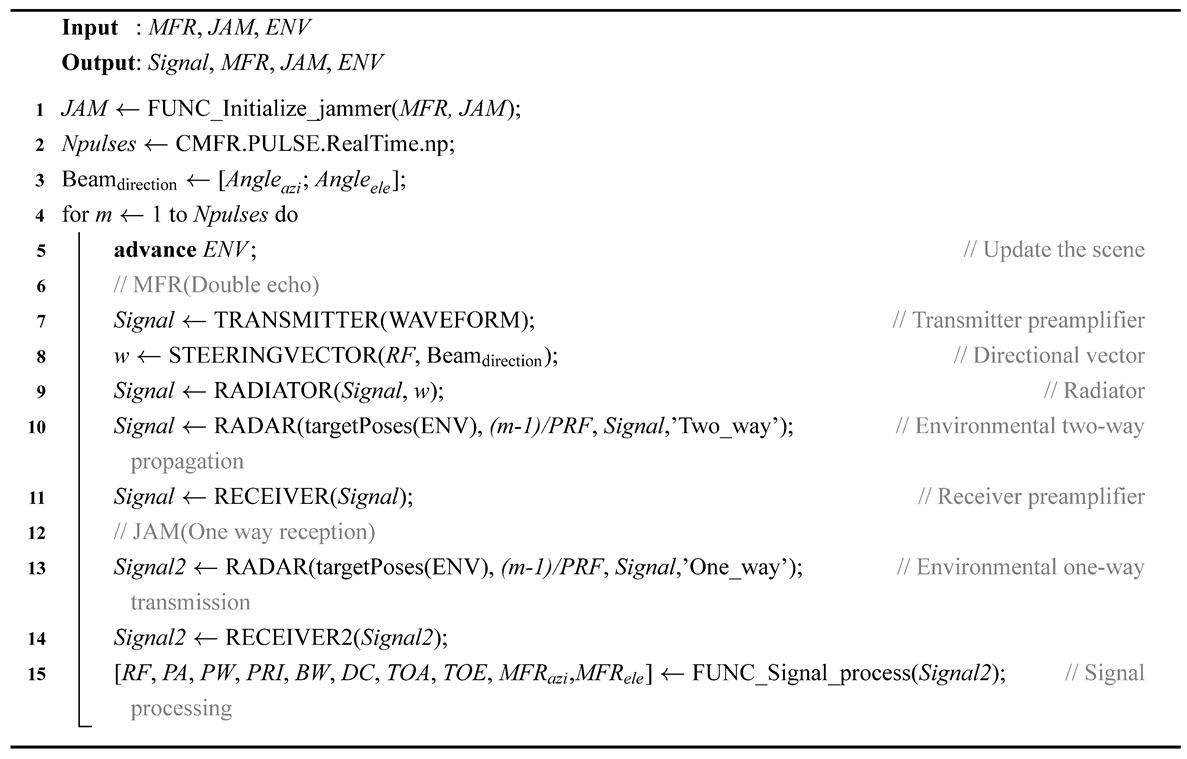
First, analyze the function FUNC_Generate_echos. As illustrated in Appendix H, MFR interacts with JAM within this function. Initially, MFR generates a signal via the transmitter preamplifier and acquires a guiding vector based on the beam azimuth angle. Subsequently, it emits the signal from the radiator which undergoes one-way propagation in ENV before being intercepted by JAM and completing two-way propagation to obtain echo signals through MFR’s receiver preamplifier.
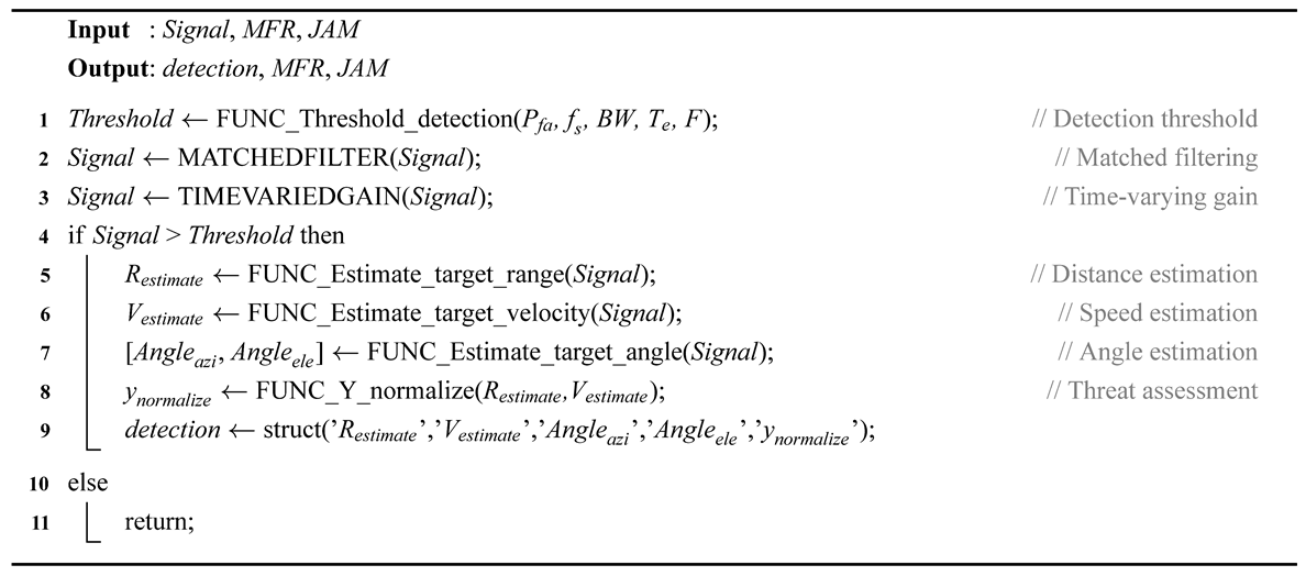
Next, we analyze the function FUNC_Generate_detections. The output S i g n a l obtained in Appendix H serves as the input for Appendix I and undergoes matched filtering and time-varying gain before undergoing a detection threshold decision. If it fails to surpass the detection threshold, the function terminates and proceeds to execute the subsequent state; however, if it exceeds the detection threshold, signal processing is conducted to derive estimated values of distance, velocity, and angle while simultaneously calculating a threat assessment value.

3.2.3. MFR External Behavior

The behavioral analysis in Section 3.2.1 and Section 3.2.2 is conducted from the MFR perspective, while the explicit behavioral analysis in this section is approached from the JAM perspective, which relates to the data characteristics after signal processing in Section 3.1.4.
According to Section 3.2.2, the interaction between MFR and JAM occurs within the function FUNC_Generate_echos, enabling direct extraction of specific external behavioral characteristics such as signal amplitude from the received signals. Considering significant gain disparities between the main lobe and side lobes of JAM’s received signal from MFR, further signal processing facilitates acquisition of PDW parameters for the MFR signal along with its physical location and angle information. By evaluating MFR’s external behavior comprehensively, we can analyze its temporal behavioral characteristics and infer implicit behavior accordingly. The evaluation results of overt behavior will be thoroughly analyzed in experimental Section 4, with a focus on the detailed examination and interpretation of the obtained outcomes.

4. Experiments and Results

The temporal behavior of AMFR is analyzed in this section through simulation experiments, which consists of two parts:
  • Constructing simulation scenarios for MFR, JAM, and ENV. An adaptive resource management and task scheduling framework is introduced to simulate AMFR in MFR. For JAM, reconfigure the composition and parameters of the deployed reconnaissance team. The physical spatial positions of MFR and JAM as well as their respective environmental parameters are defined in ENV.
  • The simulation system autonomously generates signal flow data with temporal characteristics and stores the processed data in a pulse stream format. The temporal dynamics within the pulse flow data are revealed by conducting an analysis following the interaction between both parties.

4.1. Simulation Parameter Settings

The partial simulation parameters for MFR, JAM, and ENV can be found in Appendix B. In MFR, the constant values are directly provided in the table, while the time-varying values change dynamically based on variations in ENV’s parameters. The structure of each component within the uppercase-named operational processes is outlined in MFR. For JAM, this simulation primarily focuses on spatial positioning and target quantity; signal detection and processing stages are not emphasized or elaborated upon in this paper. Finally, simulations are conducted in the ENV for spatial scenarios, environmental channels, and platform parameters of MFR and JAM.
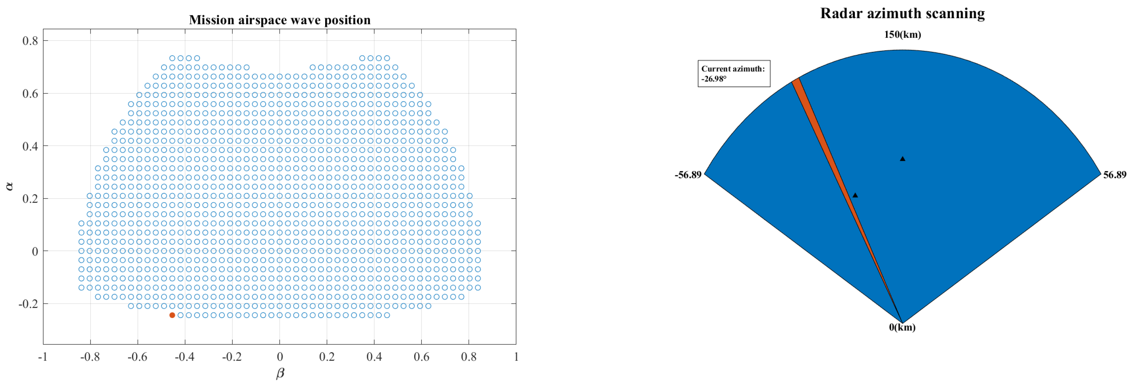
The system simulation is in progress, and the visualization presents the perspective of MFR. Figure 2 (left) illustrates the spatial waveform arrangement diagram of MFR’s tasks under the current simulation parameters, while Figure 2 (right) showcases a top-down view of the scanning spatial domain. In this depiction, MFR’s beam is positioned at its initial state, with a black triangle indicating the simulated JAM target.

4.2. Temporal Behavior Analysis

The visual observation in Figure 2 demonstrates that MFR accurately simulates the real-time spatial positioning of JAM while performing a series of tasks within the designated area. The system operates autonomously without unnecessary human intervention once it is initialized. In the system operation, each pulse point is assigned a label indicating the current simulation time to establish temporal ordering correlation among them. The management behavior of MFR is executed at the functional level, without delving into the pulse and signal levels. The switching criteria for working modes and states can be intuitively obtained from Appendix A, avoiding excessive details here. Subsequently, this paper primarily analyzes the evaluation behavior of MFR and assesses its external manifestations.

4.2.1. Evaluation Behavior Analysis of MFR

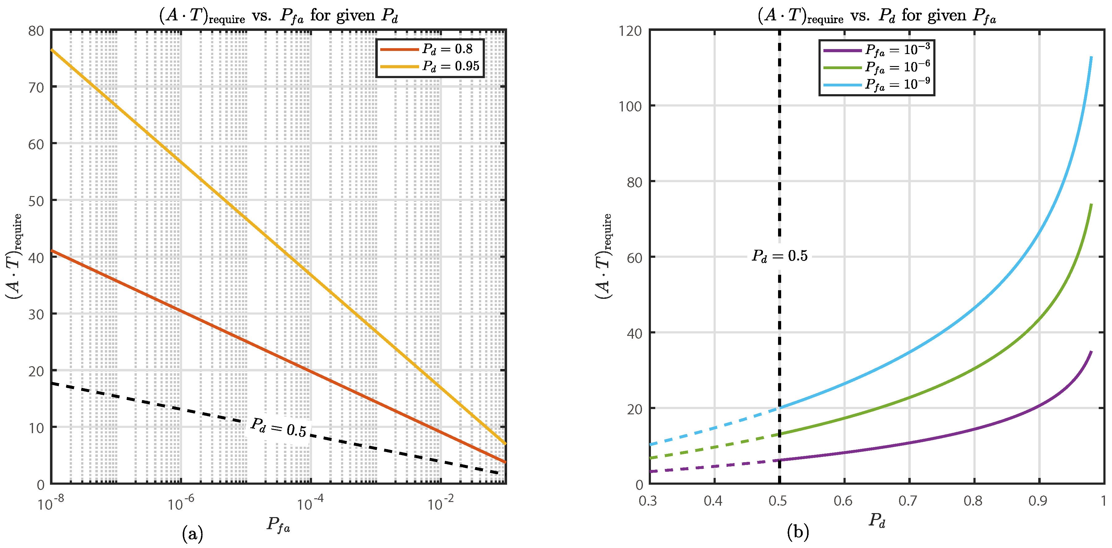
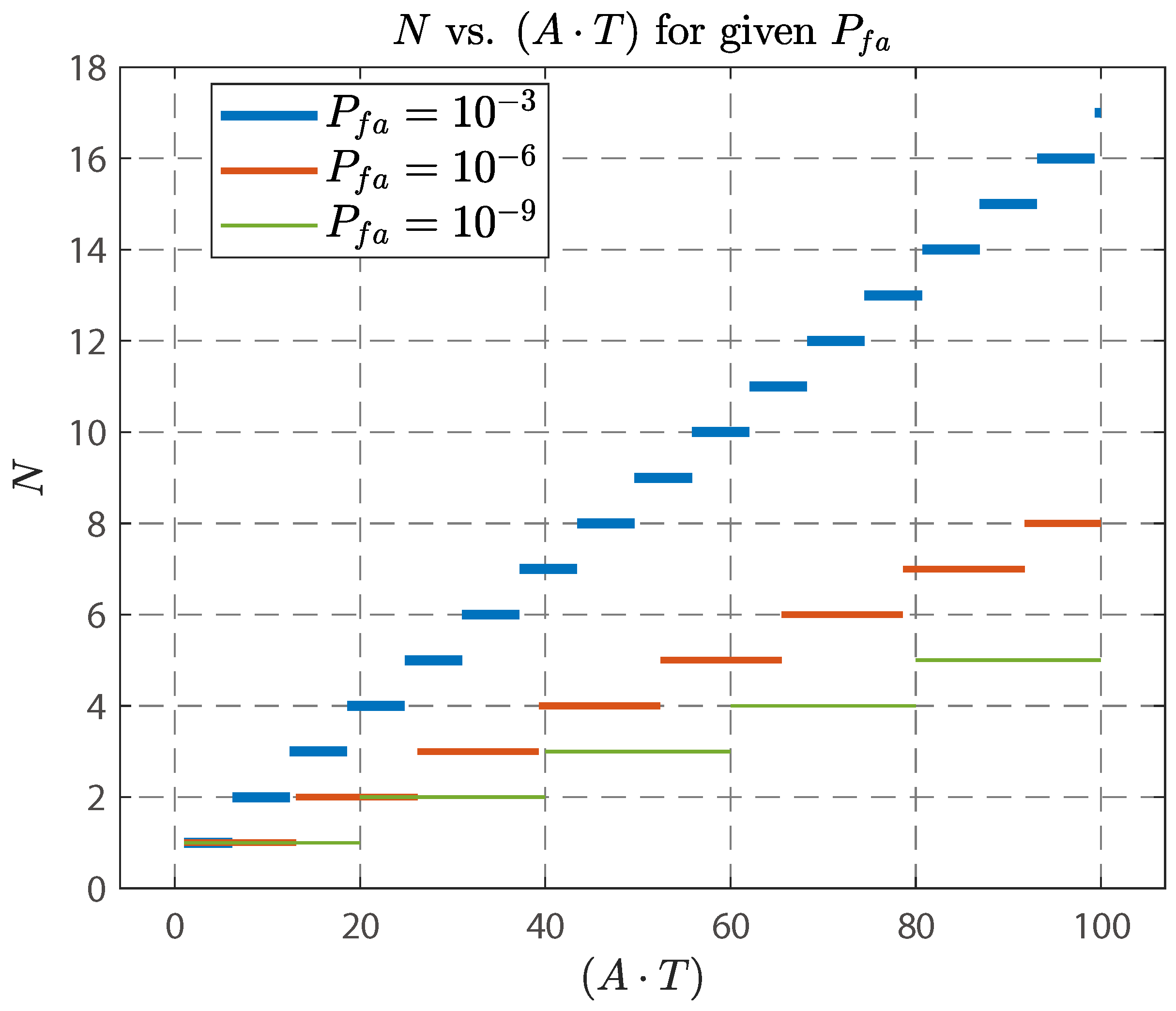
In Section 3.1.1, we conducted an analysis of the adaptive resource management and task scheduling framework of MFR, focusing on the evaluation behavior primarily manifested in the processing and analysis of echo signals, which directly impact the generation of MFR waveform parameters. By utilizing Equation (10), we derived the relationship between the value of A · T require in state S and P d as well as P f a . In the provided initial configurations of P d and P f a , Figure 3a illustrates the trend curve of A · T require with respect to P f a , while Figure 3b presents the trend curve of A · T require in relation to P d . Only three specific scenarios are presented for the other variable in each depicted relationship equation. Furthermore, Figure 4 illustrates the relationship curve between the number of pulses emitted by MFR (N) and A · T , based on the current optimal pulse parameter settings. Once MFR completes setting the waveform parameters, it concludes the evaluation behavior and transitions to management behavior to determine the working mode and status of the subsequent task sequence.

4.2.2. Outward Behavior Assessment of MFR

The outward behavior of MFR, as defined in reference [1], refers to radar external activities that can be directly observed, measured, and recorded by the detecting party. These behaviors serve specific purposes and are essential for fulfilling radar detection functions; hence they are referred to as outward behavior. In this paper, the pulse signals emitted by MFR are intercepted by JAM after spatial transmission through ENV. The input signal passing through JAM undergoes stages of signal detection, parameter estimation, and signal sorting before being outputted in the form of PDW. Along with PDW, real-time obtainable information includes the azimuth angle, elevation angle, distance between MFR and JAM, as well as radial velocity of JAM relative to MFR.
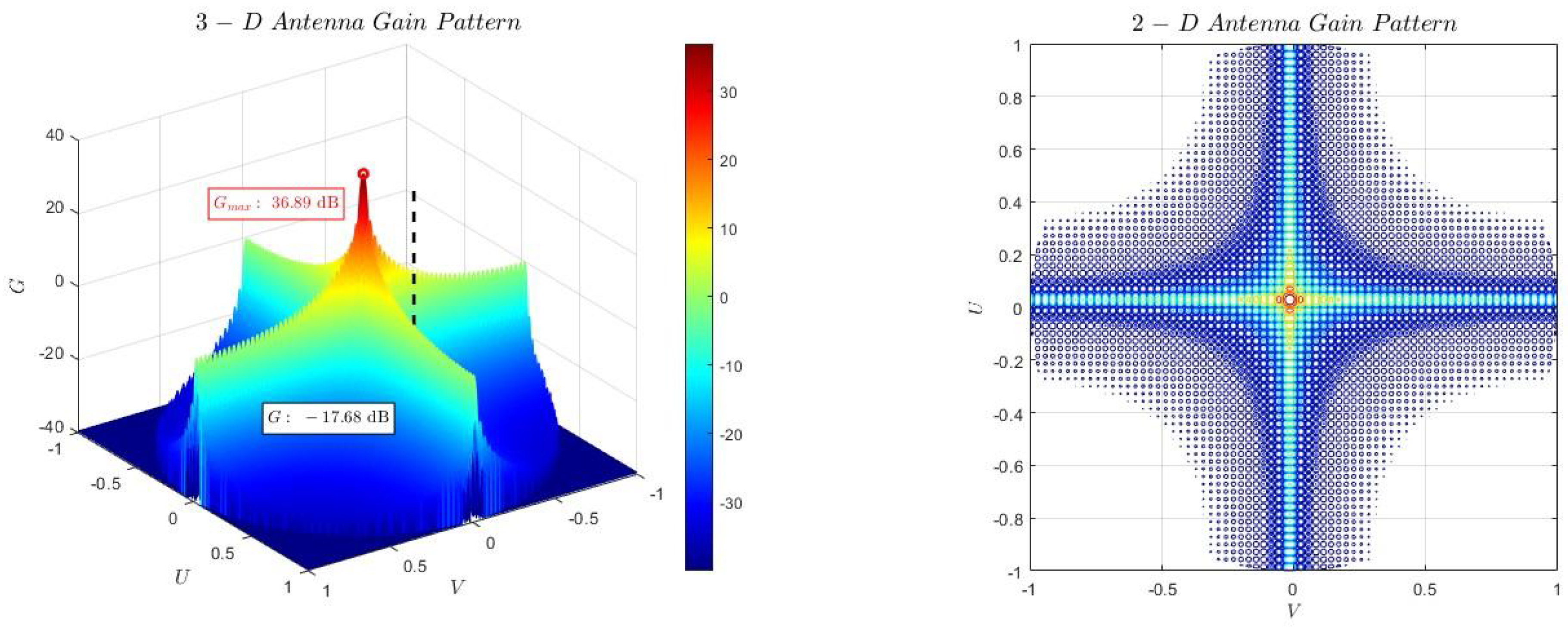
The signal strength captured by JAM is determined by the directional pattern of the antenna array during the two-dimensional phase scan with MFR. Figure 5 illustrates the three-dimensional and two-dimensional gain patterns of the antenna array at a specific moment when MFR transmits signals, achieving a maximum gain G max of 36.89 dB. In the U-V space, JAM exhibits a radiation gain G relative to MFR of −17.68 dB. However, due to ENV propagation, the received signal becomes contaminated with noise, leading to a rapid increase in errors during signal processing and rendering it impractical and devoid of value.
Under the parameter conditions specified in Appendix B, we extracted the signal flow data corresponding to the MFR’s first execution of the S state within the designated time period and plotted the frequency spectrum in a noise-free environment, as shown in Figure 6. This figure illustrates the optimal waveform parameters that, according to the mathematical model and the established operational mechanism of the MFR, achieve the desired detection probability P d and false alarm probability P f a under theoretical conditions. As depicted, the number of transmitted pulses n p = 5 , after non-coherent accumulation of the pulse echoes, precisely meets the minimum required SNR under interference-free conditions. In our current ENV environment, the remaining waveform parameters are as follows: carrier frequency R F = 1.3 GHz, pulse width P W = 500.63   µ s, bandwidth B W = 1.499 MHz, pulse repetition frequency P R F = 799 Hz, sampling rate f s = 2.998647 10 6 , pulse repetition interval P R I = 1.3 10 3 s and time-bandwidth product P C R = 751 . If a more complex electromagnetic environment exists within ENV, the current waveform parameters may be obscured by clutter or interference. Consequently, the MFR must recalculate and determine the transmitted pulse waveform parameters based on the mathematical model in order to accomplish the corresponding tasks.
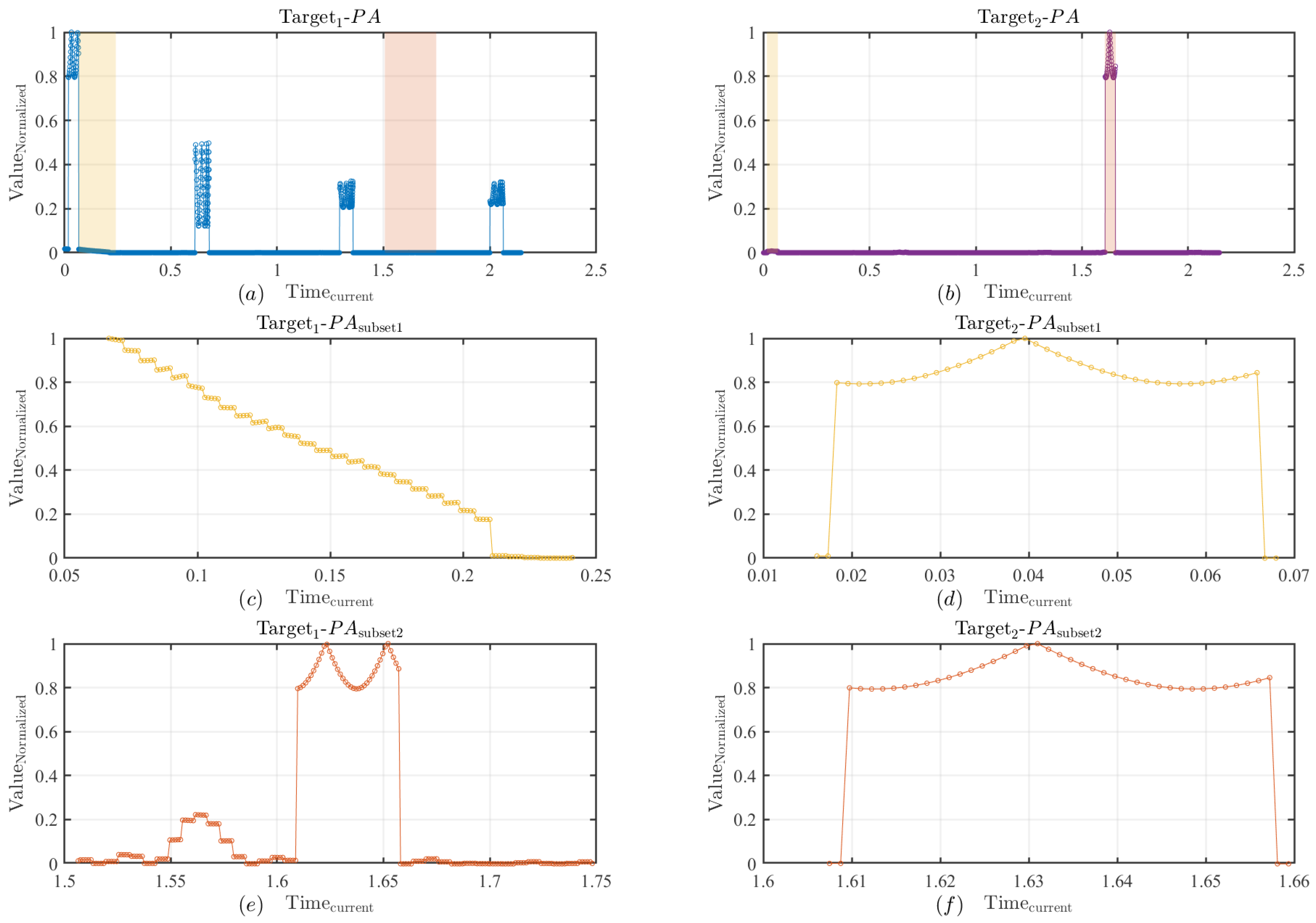
Under identical external conditions, JAM detects MFR in the ENV environment with a detection time of 2.15 s for both Targe t 1 and Targe t 2 . Figure 7a displays the temporal amplitude graph of the signal obtained when MFR detects Targe t 1 . Initially in state S, MFR switches to state C upon detecting Targe t 1 , and the first peak observed in Figure 7a represents the pulse signal emitted by MFR in state C. It is evident that this peak fluctuates due to variations in antenna array gain caused by relative motion between Targe t 1 and MFR at the current angle.
Consequently, the MFR consistently executes the S state in the task space and transitions to the T state when it meets the ’look-back’ condition, thereby achieving target tracking for newly added targets. The peak amplitude of PA following state C in Figure 7a represents the pulse signal generated by MFR during its execution of T state for Targe t 1 . The variation in signal amplitude is attributed to discrepancies between predicted and actual positions of Targe t 1 after completing the T state. Figure 7c illustrates a subset of signals with colors corresponding to those marked in Figure 7a, indicating a significant decrease in gain within this specific signal interval.
The time-domain plot of the signal amplitude obtained by Target 2 during MFR signal detection, represented in Figure 7b, exhibits similarity to Figure 7a. The peak value in the PA region of this graph signifies the emitted signal waveform generated by MFR when detecting and executing state C on Target 2 . We have extracted corresponding time intervals for MFR’s execution of state C on both Target 1 and Target 2 , as depicted in Figure 7d and Figure 7f respectively. From these graphical representations, it is evident that when MFR’s guidance vector points towards Target 1 for emitting a signal, simultaneously, Target 2 detects a signal with identical waveform parameters. Due to the spatial separation between Target 1 and Target 2 , there exists a minimal time difference in their respective signal detections amounting to approximately 6.1 × 10 5 seconds under the current ENV scenario.
We extract waveform parameters of MFR acquired through signal reconnaissance on Target 1 in JAM. Figure 8 illustrates the carrier frequency ( R F ), pulse width ( P W ), pulse repetition interval ( P R I ), bandwidth ( B W ), distance between the target and MFR ( D I S ), and elevation angle of MFR ( A n g l e ele ). In our self-adaptive resource management and task scheduling framework proposed in this study, the central position of MFR’s task spatial wave corresponds to the radiation direction of the main beam of the antenna array. Additionally, it can be observed that each waveform parameter depicted in Figure 8 is a fusion outcome derived from multiple target reconnaissances. During the current time period, MFR executed one C state and three T states on Target 1 , while only one C state was performed on Target 2 . Consequently, within this time frame, the level of threat posed by MFR to both Target 1 and Target 2 differs.
Figure 8a–c visually illustrate the parameter variations of MFR emission signals over time when MFR operates in C or T states at transition points. As shown in Figure 7, some transition points exhibit more pronounced amplitudes in Figure 7a, while others show greater amplitudes in Figure 7b. This difference is attributed to MFR’s current operation mode of TAS, which involves simultaneous tracking of Target 1 and Target 2 . During sidelobe reconnaissance when the target is not illuminated by the main beam, signal energy is low, as seen in Figure 7e, corresponding to the red shaded area in Figure 7a. However, waveform parameters from MFR can still be observed after local amplification. If environmental clutter noise is added to Figure 7e, it may be overwhelmed by clutter signals and become undetectable by JAM. When the target is illuminated by the main beam, significant gain enhancement compared to sidelobe reconnaissance can clearly be observed from Figure 7a,b.
The received RF, PW, and PRI parameters in Figure 8a–c exhibit abrupt changes, indicating their non-static nature. This is attributed to the adaptive resource management and task scheduling employed by MFR based on real-time information such as target distance and velocity when encountering different JAM targets in ENV. As a result, a harmonious balance between waveform parameters, emission time resources, and energy resources is achieved.
Based on the aforementioned simulation results, it is evident that diverse objectives and states of JAM have a substantial influence on MFR’s behavior within the ENV environment. Consequently, when analyzing MFR’s behavior, it becomes imperative to concurrently consider the state information of JAM. Furthermore, due to receiving sparse and localized signals from MFR frequently, incorporating temporal features into the analysis of MFR’s behavior becomes necessary. The simulation experiments in this section start from JAM’s perspective and demonstrate that accurately recognizing patterns solely through signal interception presents challenges for understanding MFR’s dynamics. This finding reinforces our previous assertion that for reconnaissance purposes, real-time analysis of MRF’s behavior proves more effective than solely focusing on the characteristics of radar working modes at present moments.

4.2.3. Analysis on the Applicability of MFR

The waveform parameters emitted by MFR were visually observed in Section 4.2.2, and the task sequence executed based on its determined intrinsic mechanism in a specific ENV scenario was analyzed through simulation analysis. From the JAM perspective, an increase in quantity would augment the complexity of the ENV scenario; however, from the MFR standpoint, due to its adaptive mechanism within the model, an escalation in target quantity and airspace complexity does not exhibit a significant proportional relationship. According to Equation (26), MFR assesses threats based on real-time distance and the velocity information of targets and subsequently determines next “look-back” time and T-state execution time according to real-time threat evaluation results.
Even if there are numerous targets present in the target airspace, certain targets that are considered low-threat by the MFR due to their distance from the MFR or their low radial velocity will not be allocated additional resources. During adaptive resource management and task scheduling, the primary influencing factor for the MFR is not solely based on the quantity of multiple targets in the airspace but rather focuses on the overall re-balancing and allocation of resources based on signal echoes. In Section 4.2.2, we only present one scenario to illustrate how the MFR executes the LRS and TAS modes without analyzing additional target scenarios. The suitability of an MFR system is determined not by its ability to handle a specific number of targets or complexity of target behavior in an environment, but rather by its inherent mechanism for managing resource constraints.
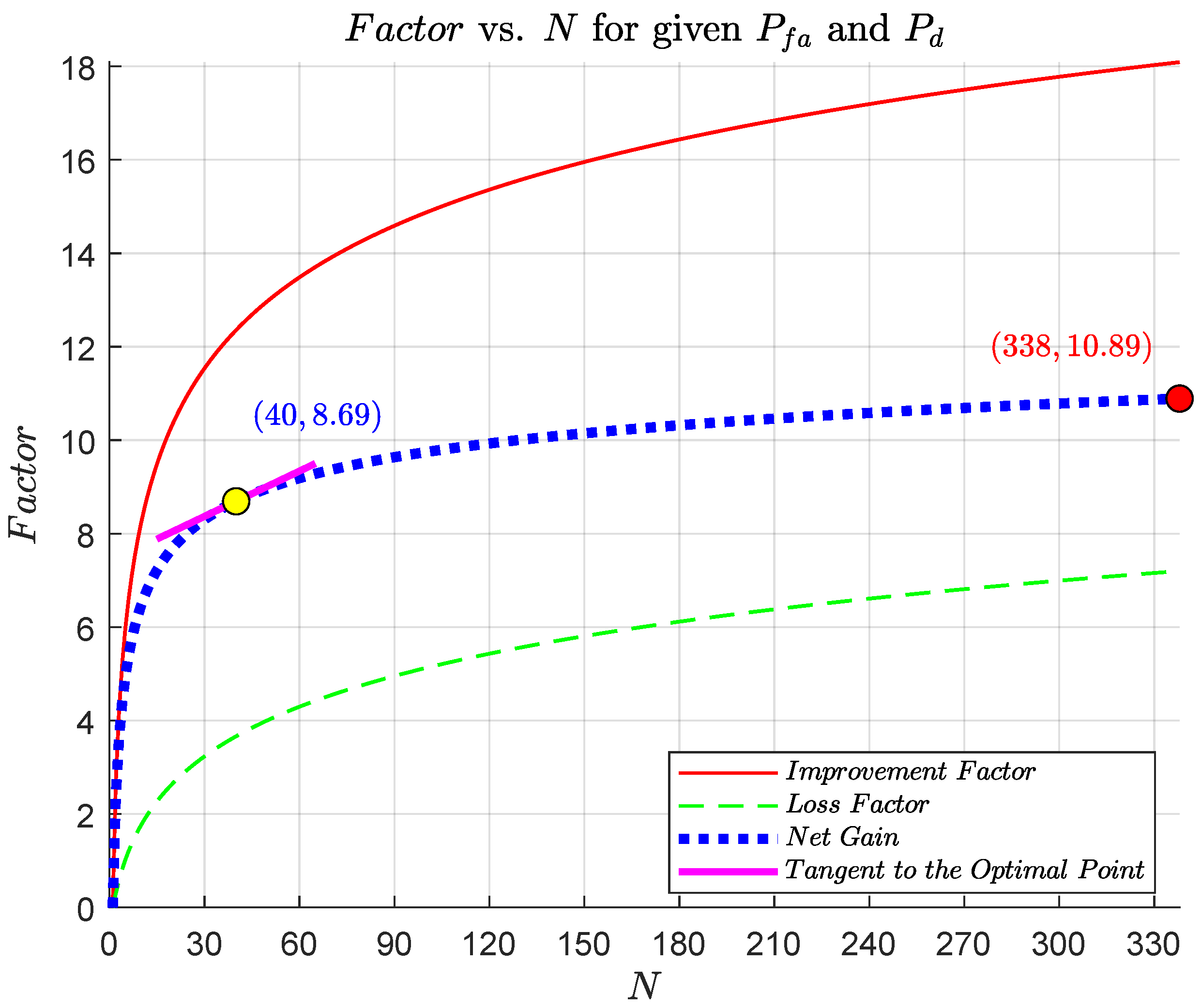
Figure 9 shows the improvement factor, loss factor, net gain variation curve, and the optimal point tangent line. Point (40,8.69) in the figure represents the optimal number of pulses and the net gain value of incoherent accumulation. Under the constraint of φ , at this time N c o n f i r m _ m a x = 338 and F a c t o r net N confirm _ max = 10.89 are obtained, and further obtaining E v a = 0.4236 . This E v a value is the max E v a under the current parameter values. The current system parameter settings allow MFR to dynamically adjust the number of transmitted pulses within a range of 40 to 338, based on the status information of target echoes. This adaptive approach aims to achieve a maximum net gain of 10.89 dB.
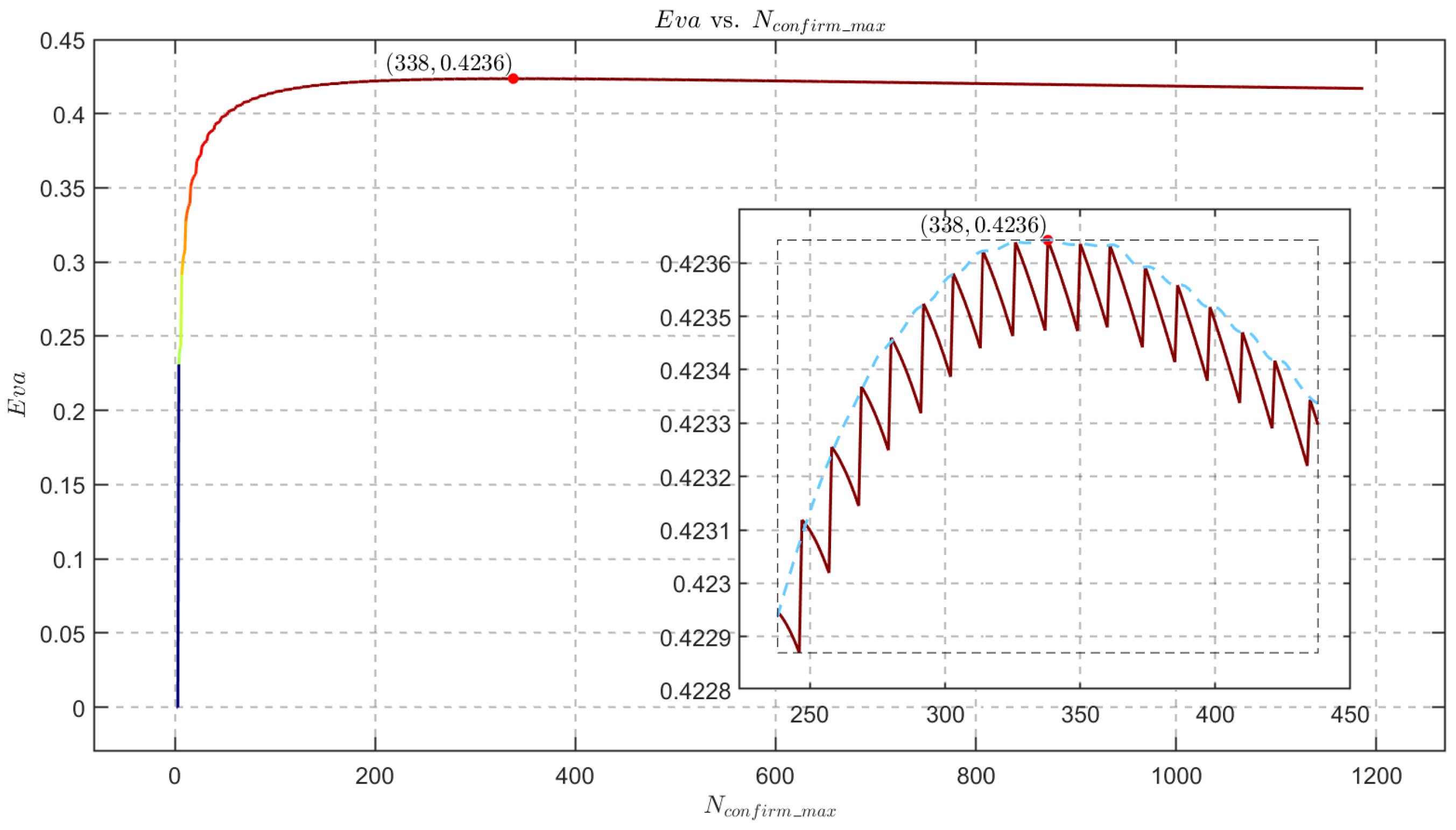
Figure 10 shows the trend curve of the E v a value for different N c o n f i r m _ m a x values. It can be seen that the curve first rises and then falls, with the maximum value corresponding to the coordinate point (338,0.4236). The embedded local magnification shows the trend of the curve near the maximum value. Based on N c o n f i r m _ m a x and T f r a m e , we can obtain the optimal φ = 5.7 % . Simultaneously, we can validate that under non-ideal environmental conditions, the model has the capability to dynamically optimize the number of emitted pulses N c o n f i r m _ m a x in order to meet real-time SNR requirements.
We acknowledge that the characteristics of working modes are determined by the internal mechanisms of MFR. Under identical working modes, MFR can exhibit distinct waveform parameters and task sequence features. The simulation results presented in this section demonstrate the applicability and real-time performance of adaptive resource management and task scheduling executed by AMFR when confronted with complex spatial domains from an MFR perspective.

5. Discussion

The article addresses the issues of waveform parameter variability and behavioral flexibility in the presentation of AMFR behavior within the context of MFRBA. A digital radar simulation system is constructed to autonomously generate resource management and task scheduling based on simulated AMFR real behavior. In contrast to traditional methods that rely on manually setting waveform parameter ranges, this system incorporates an adaptive framework for resource management and task scheduling within MFR. JAM simulates both the cross-section area and behavioral mode of real targets, enabling dynamic updates of the ENV scene for the first time, with its update rate synchronized with that of MFR. At this update rate, ENV synchronously updates MFR and JAM during each pulse period execution, ensuring a high level of consistency between the simulation environment and radar behavior.
In recent years, DL has shown exceptional performance in analyzing radar behavior. However, existing research often oversimplifies the simulation of radar behavior by only using diverse pulse descriptor parameters to illustrate the radar’s operational mode and state transitions. This approach overlooks the temporal ordering relationship of pulse streams, resulting in a lack of crucial time labels and ordering information within signal flows. As a result, during training, there is a high risk of overfitting due to reliance on artificially generated differentiated signals rather than authentic pulses and missed pulses present in real signal flows. Moreover, such dependence on human-generated variations makes the network’s analysis results more susceptible to bias. For example, AMFR resource management and task scheduling rules exhibit extensive waveform parameter variations and dynamic variability of beam “look-back” time under Task Adaptive Scheduling (TAS) mode. From an MFR perspective, the radar adapts its working state through adaptive switching within the same operating mode to accomplish different tasks with identical waveform parameters; whereas from a JAM perspective, diversity in waveform parameters may be misinterpreted as different working modes. If network training solely relies on pulse streams without time labels when encountering completely new unknown sample signals, it may excessively prioritize classification outcomes while disregarding crucial temporal information within signal flows—ultimately leading to significant performance degradation that fails to meet practical requirements.
By leveraging the interaction between MFR and JAM in the environment, this study achieves interpretability of MFR’s behavior in various spatial environments. Within the adaptive resource management and task scheduling framework of MFR, emitted waveform signals are analyzed based on the received data parameters from a JAM perspective. Comparative analysis of target signal stream data indicates that during MFRBA, both amplitude information and its time label should be considered as important factors. By annotating time labels to amplitude information within the signal stream, attention can be reduced towards signal intervals containing waveform parameters of interest but with less importance in terms of amplitude information. For example, when the radar main beam illuminates target two while target one receives similar signal parameters through sidelobes, these signal parameters hold lower value for target one and should be weakened in temporal behavior analysis; whereas for target two, these signal parameters need to be strengthened. Through simulation experiments at a signal-level hierarchy, we draw the following conclusions:
  • Different perspectives on differences: The areas of interest between MFR and JAM exhibit disparities from different perspectives. MFR primarily focuses on comprehensive control and optimization of internal resource management, as well as task scheduling mechanisms, with the objective of enhancing radar efficiency in resource utilization and task execution capability. Conversely, JAM places emphasis on real-time evaluation of behavioral threats posed by MFR, specifically highlighting the detection and identification of potential impacts on environmental targets resulting from radar behavior.
  • The importance of key temporal information: In the MFRBA process, the amplitude information of signals with time stamps plays a crucial role that cannot be overlooked. Different targets may exhibit distinct temporal characteristics even when receiving identical waveform parameters. By integrating detection results from multiple devices, signal leakage caused by sidelobe attenuation in individual devices can be compensated for, thereby enhancing the integrity and precision of temporal pulse flow analysis.
Based on the above research, this paper presents a more precise and reliable analysis approach for MFRBA, thereby advancing the progress of radar behavior recognition technology and establishing a robust foundation for behavior analysis in complex radar systems. In the future, we can focus on two aspects:
  • Multi-machine collaborative fusion: The accuracy and robustness of the overall analysis are enhanced through real-time collaborative fusion of data from multiple machines, enabling comprehensive behavioral analysis of single or even multiple radars.
  • Pulse flow temporal correlation modeling: Incorporating time correlation modeling of pulse streams into deep learning network structures can effectively mitigate uncertainty in behavior analysis, thereby enhancing the accuracy and reliability of analysis given the sparse and localized nature of effective radar signals in signal flow.

Author Contributions

Conceptualization, Z.X. and Q.Z.; methodology, Z.X. and J.Q.; validation, Z.L. and Q.C.; investigation, Z.X. and Y.D.; writing—original draft preparation, Z.X., J.Q. and Q.X.; writing—review and editing, Z.X., Y.D., Q.X. and Q.C.; supervision, Z.X. and Z.L.; project administration, Z.L. and Q.Z.; funding acquisition, Z.L. All authors have read and agreed to the published version of the manuscript.

Funding

This research is partly supported by the National Natural Science Foundation of China under Grants 62301581 and the China Postdoctoral Science Foundation under Grants 2023M734313.

Data Availability Statement

The data are available to readers by contacting the corresponding author.

Acknowledgments

The authors would like to thank all of the reviewers and editors for their comments on this paper.

Conflicts of Interest

The authors declare no conflicts of interest.

Appendix A. Working Pattern Closed-Loop Switching Diagram
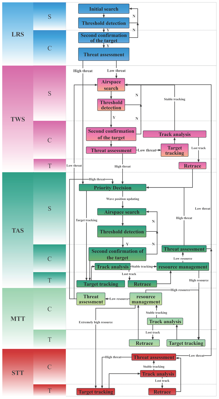
Remotesensing 16 04131 i001

Appendix B. Simulation Parameter Information Table

Variable SymbolDefinitionVariable ValuesVariable SymbolDefinitionVariable Values
MFRcSpeed of light3 × 10 8 (m/s)kBoltzmann constant1.38 × 10−23
T e Noise temperature290 (k) M a x f r a m e Maximum frame count/
T i m e c u r r e n t Current time/ P d Detection probability 0.95
T f r a m e Frame period/ N u m v a l i d Number of effective wave positions/
M a x t r a c k Maximum tracking number/ P f a False alarm probability1 × 10−6
Δ R search S state range resolution100 (m) R max _ search S state unambiguous range150 (km)
Δ R confirm C state rr100 (m) R max _ confirm C state ur150 (km)
Δ R track T state rr100 (m) R max _ track T state ur/
V max _ search S state unambiguous velocity/ A n g l e azi Target azimuth angle/
V max _ confirm C state uv343 (m/s) A n g l e ele Target elevation angle/
V max _ track T state uv343 (m/s) A n g l e center Central azimuth angle0 (°)
A n g l e max _ azi Max azimuth angle π 3 (rad) A n g l e max _ ele Max elevation angle π 3 (rad)
A n g l e min _ ele Min elevation angle0 (°) B e a m 3 dB _ azi Level 3 dB beamwidth/
R estimate Distance estimation/ B e a m 3 dB _ ele Vertical 3 dB beamwidth/
V estimate Velocity estimation/ X array X-axis quantity70
y normalized Threat value/ Y array Y-axis quantity70
GGain of antenna array/ C h a n n e l Number of channels4900
FNoise factor7 (dB) L o s s Radar loss7 (dB)
R C S s t a n d a r d Reference RCS10 (m2) f standard Reference RF1.3 GHz
P t Peak power100 kw P R F Pulse repetition frequency/
R F Radio frequency/ P R I Pulse repetition interval/
P W Pulse width/ D C Duty cycle/
B W Band width/ P C R Pulse compression ratio/
Pattern 1 Pattern oneLRS Pattern 2 Pattern twoTWS
Pattern 3 Pattern threeTAS Pattern 4 Pattern fourMTT
Pattern 5 Pattern fiveSTT State 1 State oneS
State 2 State twoC State 3 State threeT
TRANSMITTER Transmitter preamplifier/ RECEIVER Receiver preamplifier/
RADIATOR Radiator/ COLLECTOR Collector/
WAVEFORM Signal waveform/ RADAR Radar transceiver/
MONOPULSE Monopulse measuring apparatus/ MATCHFILTER Matched filter/
TIMEGAIN Time varying gain/ TRACKER Tracker/
JAM T a r g e t n u m Target quantity/ N a m e I D Target number
R C S Radar cross section/ P o s i t i o n Target location/
V e l o c i t y Target velocity/ X array X-axis quantity/
R F Working frequency/ Y array Y-axis quantity/
f s Sample frequency/
ENV SCENE Scene/ CHANNEL Channel/
PLATFOR M Radar Radar platform/ PLATFOR M Target Target platform/

Appendix C. The Design of Waveform Parameters for LRS Mode S State
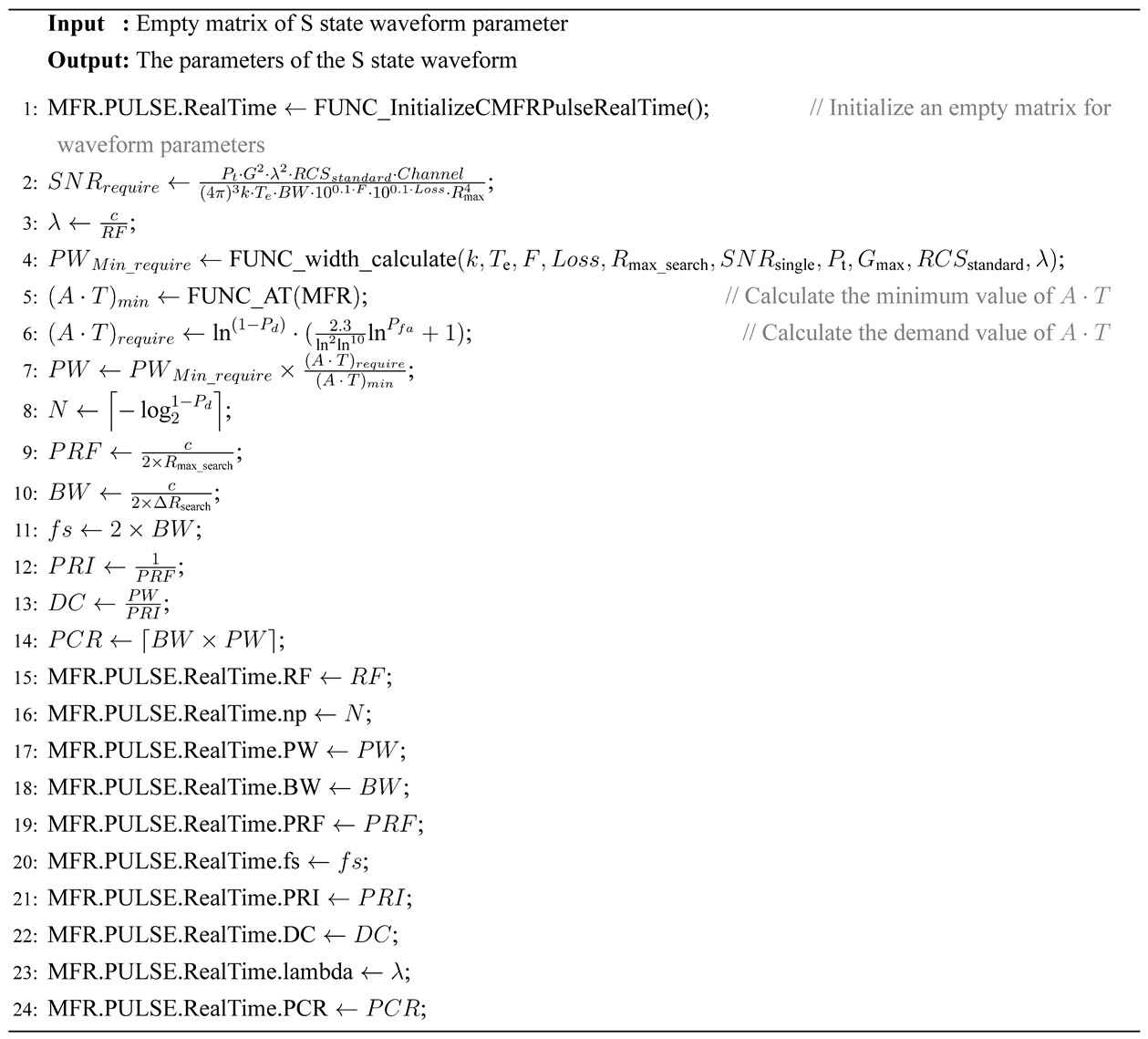
Remotesensing 16 04131 i002

Appendix D. The Design of Waveform Parameters for LRS Mode C State
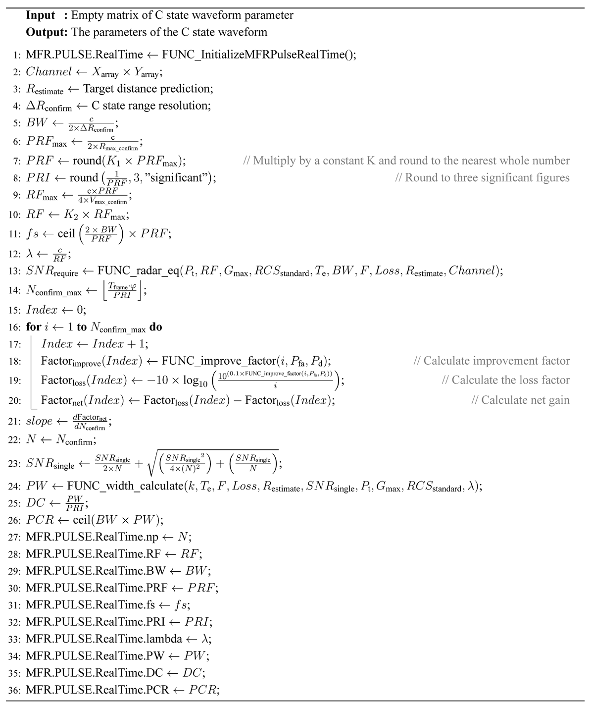
Remotesensing 16 04131 i003

Appendix E. (Left) Digital Radar Simulation System Framework. (Right) Function FUNC_Master_control

Remotesensing 16 04131 i004

Appendix F. Function FUNC_Current_radar_task
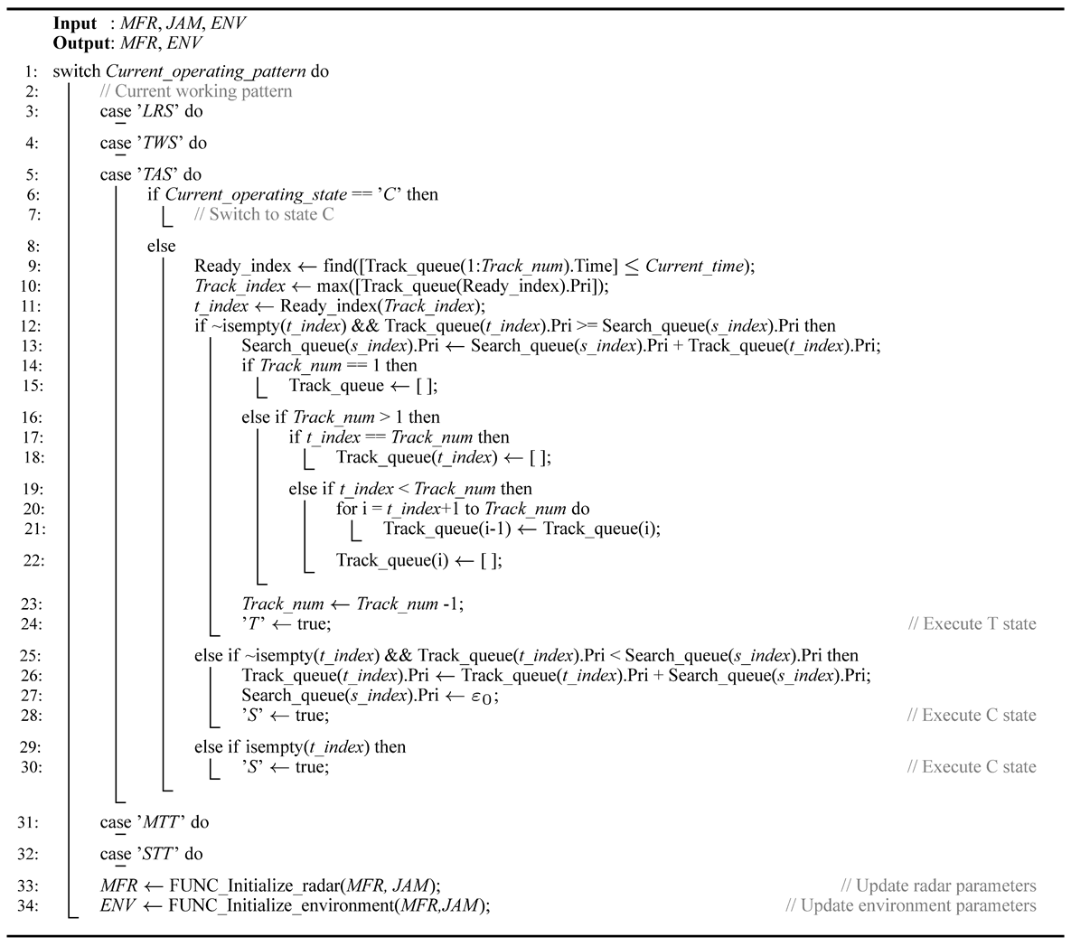
Remotesensing 16 04131 i005

Appendix G. Function FUNC_Update_job_queue
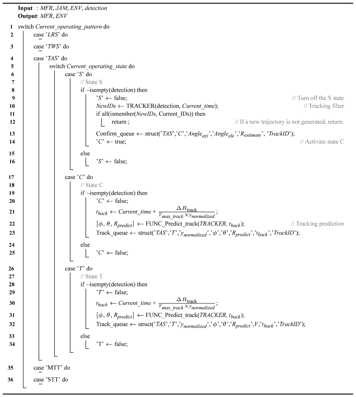
Remotesensing 16 04131 i006

Appendix H. Function FUNC_Generate_echos
Remotesensing 16 04131 i007

Appendix I. Function FUNC_Generate_detection
Remotesensing 16 04131 i008

References

  1. Wang, S.; Zhu, M.; Li, Y.; He, J.; Liang, K.; Zhang, L.; Su, K.; Ma, H.; Chen, L.; Dong, X.; et al. Recognition, reasoning, and prediction of advanced multifunction radar system behavior: Overview and prospects. Signal Process. 2024, 40, 17–55. [Google Scholar]
  2. Haykin, S. Cognitive radar: A way of the future. IEEE Signal Process. Mag. 2006, 23, 30–40. [Google Scholar] [CrossRef]
  3. Charlish, A.; Hoffmann, F.; Degen, C.; Soloviev, A.; Dale, C.; Griffiths, H. The development from adaptive to cognitive radar resource management. IEEE Aerosp. Electron. Syst. Mag. 2020, 35, 8–19. [Google Scholar] [CrossRef]
  4. Bi, Z.; Xu, C.; Zhang, X.; Lu, L. Phased Array Radar Resource Management Technology; National Defense Industry Press: Beijing, China, 2016. [Google Scholar]
  5. Martone, A.F.; Charlish, A. Cognitive radar for waveform diversity utilization. In Proceedings of the 2021 IEEE Radar Conference (RadarConf21), Atlanta, GA, USA, 10–14 May 2021; pp. 1–6. [Google Scholar]
  6. Wang, B.; Wang, J.; Song, X.; Han, Y. Research on adaptive waveform selection algorithm in cognitive radar. J. Commun. 2010, 5, 467–474. [Google Scholar] [CrossRef]
  7. Liu, H.; Yan, J.; Zhang, P.; Wei, H.; Li, S.; Jiang, T. A phased array radar resource management method for multi-task scheduling. Mod. Radar 2023, 45, 8–16. [Google Scholar]
  8. Ghadian, M.; Fatemi Mofrad, R.; Abbasi Arand, B. Robust time resource management in cognitive radar using adaptive waveform design. IETE J. Res. 2023, 69, 1070–1080. [Google Scholar] [CrossRef]
  9. Klemm, R.; Griffiths, H.; Koch, W. Novel Radar Techniques and Applications: Volume 1: Real Aperture Array Radar, Imaging Radar, and Passive and Multistatic Radar; IET Publishing: London, UK, 2017; pp. 1–500. [Google Scholar]
  10. Li, Y.; Huang, P. Radar Engineering; National Defense Industry Press: Beijing, China, 1999. [Google Scholar]
  11. Mahafza, R.B.; Elsherbeni, A.Z. MATLAB Simulations for Radar Systems Design; CRC Press: Boca Raton, FL, USA, 2003. [Google Scholar]
  12. Xiong, J.; Pan, J.; Zhuo, Y.; Guo, L. A review of radar working mode recognition methods. Mod. Radar 2023, 45, 1–10. [Google Scholar]
  13. Dong, X.; Cheng, S. Radar Working Modes Recognition Based on Discrete Process Neural Network. IOP Conf. Ser. Mater. Sci. Eng. 2018, 394, 042088. [Google Scholar] [CrossRef]
  14. Liu, H. Research on Radar Operating Pattern Recognition Based on Automatic Encoder and Gradient Lift Model. Master’s Thesis, Southwest Jiaotong University, Chengdu, China, 2018. (In Chinese). [Google Scholar]
  15. Liu, H.; Jin, W.; Chen, C. Working Pattern Recognition of Phased Array Radar Based on Noise Reduction Autoencoder. J. Syst. Simul. 2017, 29, 1960–1967. [Google Scholar]
  16. Li, X.; Liu, Z.-M.; Huang, Z. Denoising of Radar Pulse Streams With Autoencoders. IEEE Commun. Lett. 2020, 24, 797–801. [Google Scholar] [CrossRef]
  17. Vincent, P.; Larochelle, H.; Lajoie, I.; Bengio, Y.; Manzagol, P.-A. Stacked Denoising Autoencoders: Learning Useful Representations in a Deep Network with a Local Denoising Criterion. J. Mach. Learn. Res. 2010, 11, 3371–3408. [Google Scholar]
  18. Li, X.; Liu, Z.; Huang, Z. Attention-Based Radar PRI Modulation Recognition With Recurrent Neural Networks. IEEE Access 2020, 8, 57426–57436. [Google Scholar] [CrossRef]
  19. Li, Y.; Zhu, M.; Ma, Y.; Yan, J. Work Modes Recognition and Boundary Identification of MFR Pulse Sequences with a Hierarchical Seq2Seq LSTM. IET Radar Sonar Navig. 2020, 14, 1343–1353. [Google Scholar] [CrossRef]
  20. Fang, Y.; Zhai, Q.; Zhang, Z.; Yang, J. Change Point Detection for Fine-Grained MFR Work Modes with Multi-Head Attention-Based Bi-LSTM Network. Sensors 2023, 23, 3326. [Google Scholar] [CrossRef]
  21. Fan, J.; Wu, L.; Zhang, J.; Dong, J.; Wen, Z.; Zhang, Z. Deep Learning-Aided Modulation Recognition for Non-Orthogonal Signals. Sensors 2023, 23, 5234. [Google Scholar] [CrossRef]
  22. Tang, W.; Long, G.; Liu, L.; Zhou, T.; Blumenstein, M.; Jiang, J. Omni-scale CNNs: A Simple and Effective Kernel Size Configuration for Time Series Classification. In Proceedings of the International Conference on Learning Representations, Virtual, 25–29 April 2022. [Google Scholar]
  23. Pan, J.; Zhang, S.; Xia, L.; Tan, L.; Guo, L. Embedding Soft Thresholding Function into Deep Learning Models for Noisy Radar Emitter Signal Recognition. Electronics 2022, 11, 2142. [Google Scholar] [CrossRef]
  24. Qiao, J.; Yue, X. Multi-label Recognition of Radar Radiation Source Based on Improved Residual Network. Mod. Radar 2022, 44, 39–44. (In Chinese) [Google Scholar]
  25. Han, Z. Radar Data Fusion Tracking and Working Pattern Recognition. Master’s Thesis, Xidian University, Xi’an, China, 2019. (In Chinese). [Google Scholar]
  26. Chen, X.; Qiu, P.; Zhu, W.; Li, H.; Wang, H.; Sotiras, A.; Wang, Y.; Razi, A. TimeMIL: Advancing Multivariate Time Series Classification via a Time-aware Multiple Instance Learning. arXiv 2024, arXiv:2405.03140. [Google Scholar]
  27. Yu, X.; Ji, K.; Li, H.; He, Y.; Qi, H.; Cui, G. Multi-function radar work mode recognition based on clustering data annotation. Inf. Countermeas. Technol. 2023, 2, 29–46. [Google Scholar]
  28. Fu, Y.; Huang, J.; Wang, J.; Dang, T.; Li, Y.; Sun, Z. Overview of multifunction phased array radar behavior recognition. Telecommun. Eng. 2024, 64, 643–654. [Google Scholar]
  29. Ma, S. Research on Key Technologies of Multifunction Radar Electronic Intelligence Signal Processing. Ph.D. Thesis, National University of Defense Technology, Changsha, China, 2013. [Google Scholar]
  30. Ou, J. Research on Behavior Recognition and Prediction Technology of Multifunction Radar. Ph.D. Thesis, National University of Defense Technology, Changsha, China, 2017. [Google Scholar]
  31. Liu, Z.; Yuan, S.; Kang, S. Semantic coding and model reconstruction of multifunctional radar pulse train. J. Radars 2021, 10, 559–570. [Google Scholar]
  32. Pan, J.; Xiong, J.; Zhuo, Y. Working mode recognition of non-specific radar based on ResNet-SVM learning framework. Sensors 2023, 23, 3123. [Google Scholar] [CrossRef] [PubMed]
  33. Wen, Z.; Sun, M.; Tang, X.; Tian, X.; Yu, C. Multifunction radar working mode recognition based on entropy map. J. Detect. Control 2024, 46, 129–138. [Google Scholar]
  34. Liu, S.; Zhao, S.; Wang, H. New advances in radar emitter recognition technology. J. China Acad. Electron. Inf. Technol. 2022, 17, 523–533. [Google Scholar]
  35. Xu, J. Research on Radar Emitter Recognition Technology Based on Deep Learning. Ph.D. Thesis, Xidian University, Xi’an, China, 2019. [Google Scholar]
  36. Zhang, Z.; Li, Y.; Zhai, Q.; Li, Y.; Gao, M. Mode recognition of multi-function radars for few-shot learning based on compound alignments. IEEE Trans. Aerosp. Electron. Syst. 2022, 58, 5328–5342. [Google Scholar] [CrossRef]
  37. Zhai, Q.; Li, Y.; Zhang, Z.; Li, Y.; Wang, S. Few-shot recognition of multi-function radar modes via refined prototypical random walk network. IEEE Trans. Aerosp. Electron. Syst. 2022, 58, 5567–5578. [Google Scholar]
  38. Ye, F.; Zhang, W.; Gao, J.; Jiang, S. Radar small-sample working pattern recognition based on domain adaptation. In Proceedings of the 2023 IEEE 6th International Conference on Electronic Information and Communication Technology (ICEICT), Harbin, China, 9–11 September 2023; pp. 1–4. [Google Scholar]
  39. Zhao, K.; Jin, X.; Wang, Y. A survey of few-shot learning research. J. Softw. 2021, 32, 349–369. [Google Scholar]
  40. Li, Q.; Zhang, W.; Jin, Q.; Liu, K.; Sun, W.; Jiang, T.; Peng, J. Recognition of multifunctional radar working modes with small samples based on knowledge prototypical network. Acta Electron. Sin. 2022, 50, 1344–1350. [Google Scholar]
  41. Karim, F.; Majumdar, S.; Darabi, H.; Harford, S. Multivariate LSTM-FCNs for time series classification. Neural Netw. 2019, 116, 237–245. [Google Scholar] [CrossRef]
  42. Zhang, X.; Gao, Y.; Lin, J. TapNet: Multivariate time series classification with attentional prototypical network. In Proceedings of the AAAI Conference on Artificial Intelligence, New York, NY, USA, 7–12 February 2020; AAAI Press: New York, NY, USA, 2020; Volume 34, pp. 6845–6852. [Google Scholar]
  43. Fawaz, H.I.; Lucas, B.; Forestier, G.; Pelletier, C.; Schmidt, D.F.; Weber, J.; Webb, G.I.; Idoumghar, L.; Muller, P.A.; Petitjean, F. InceptionTime: Finding AlexNet for time series classification. Data Min. Knowl. Discov. 2020, 34, 1936–1962. [Google Scholar] [CrossRef]
  44. Li, G.; Choi, B.; Xu, J.; Bhowmick, S.S.; Chun, K.P.; Wong, G.L.H. ShapeNet: A shapelet-neural network approach for multivariate time series classification. In Proceedings of the AAAI Conference on Artificial Intelligence, Virtual, 2–9 February 2021; AAAI Press: New York, NY, USA, 2021; Volume 35, pp. 8365–8373. [Google Scholar]
Figure 1. Simulation system architecture.
Remotesensing 16 04131 g001
Figure 2. System-visualized operating interface.
Remotesensing 16 04131 g002
Figure 3. (a) The trend of A · T r e q u i r e under a given P d value. (b) The trend of A · T r e q u i r e under a given P f a value.
Remotesensing 16 04131 g003
Figure 4. Relationship curve between A · T and N.
Remotesensing 16 04131 g004
Figure 5. Antenna array gain pattern.
Remotesensing 16 04131 g005
Figure 6. Spectrum diagram when MFR executes the S state.
Remotesensing 16 04131 g006
Figure 7. (af) Time-domain diagram of JAM signal interception.
Remotesensing 16 04131 g007
Figure 8. (af) Signal waveform parameter diagram.
Remotesensing 16 04131 g008
Figure 9. Relationship between F a c t o r value and number of pulses N under given conditions.
Remotesensing 16 04131 g009
Figure 10. Trend of evaluation function value E v a with maximum number of pulses N c o n f i r m _ m a x .
Remotesensing 16 04131 g010
Disclaimer/Publisher’s Note: The statements, opinions and data contained in all publications are solely those of the individual author(s) and contributor(s) and not of MDPI and/or the editor(s). MDPI and/or the editor(s) disclaim responsibility for any injury to people or property resulting from any ideas, methods, instructions or products referred to in the content.