Article

Combining Sentinel-2 Data and Risk Maps to Detect Trees Predisposed to and Attacked by European Spruce Bark Beetle

Department of Physical Geography and Ecosystem Science, Lund University, 223 62 Lund, Sweden
*
Author to whom correspondence should be addressed.
Remote Sens. 2024, 16(22), 4166; https://doi.org/10.3390/rs16224166
Submission received: 24 August 2024 / Revised: 12 October 2024 / Accepted: 5 November 2024 / Published: 8 November 2024
(This article belongs to the Section Forest Remote Sensing)

Abstract

:
The European spruce bark beetle is a major disturbance agent in Norway spruce forests in Europe, and with a changing climate it is predicted that damage will increase. To prevent the bark beetle population buildup, and to limit further spread during outbreaks, it is crucial to detect attacked trees early. In this study, we utilize Sentinel-2 data in combination with a risk map, created from geodata and forestry data, to detect trees predisposed to and attacked by the European spruce bark beetle. Random forest models were trained over two tiles (90 × 90 km) in southern Sweden for all dates with a sufficient number of cloud-free Sentinel-2 pixels during the period May–September in 2017 and 2018. The pixels were classified into attacked and healthy to study how detection accuracy changed with time after bark beetle swarming and to find which Sentinel-2 bands are more important for detecting bark beetle attacked trees. Random forest models were trained with (1) single-date data, (2) temporal features (1-year difference), (3) single-date and temporal features combined, and (4) Sentinel-2 data and a risk map combined. We also included a spatial variability metric. The results show that detection accuracy was high already before the trees were attacked in May 2018, indicating that the Sentinel-2 data detect predisposed trees and that the early signs of attack are low for trees at high risk of being attacked. For single-date models, the accuracy ranged from 63 to 79% and 84 to 94% for the two tiles. For temporal features, accuracy ranged from 65 to 81% and 81 to 92%. When the single-date and temporal features were combined, the accuracy ranged from 70 to 84% and 90 to 96% for the two tiles, and with the risk map included, the accuracy ranged from 83 to 91% and 92 to 97%, showing that remote sensing data and geodata can be combined to increase detection accuracy. The differences in accuracy between the two tiles indicate that local differences can influence accuracy, suggesting that geographically weighted methods should be applied. For the single-date models, the SWIR, red-edge, and blue bands were generally more important, and the SWIR bands were more important after the attack, suggesting that they are most suitable for detecting the early signs of a bark beetle attack. For the temporal features, the SWIR and blue bands were more important, and for the variability metric, the green band was generally more important.

1. Introduction

The European spruce bark beetle (Ips typographus L.) is a main biotic disturbance agent in Norway spruce (Picea abies (L.) Karst) forests in Europe, killing several million m3 of spruce trees annually [1]. At low density populations, the bark beetles only kill weakened trees, but periodically populations grow rapidly to epidemic levels, causing large outbreaks. Such outbreaks are usually triggered by windstorms, when the bark beetles breed in storm-felled trees [2,3], or by drought events when the trees’ defense capacity is weakened [4,5]. Since a changing climate is projected to lead to higher temperatures and more frequent drought events, it is likely that there will be increasingly severe bark beetle outbreaks in the future [4,6]. In addition, longer periods with sufficiently high temperatures for the bark beetles to generate additional annual populations increase the risk of larger future outbreaks further north [7,8].
Suitable forest management strategies are needed to reduce the risk of bark beetle outbreaks. In the long term, management strategies can be applied to make forests less susceptible to the rapid growth of bark beetle populations; in the short term, management strategies aim to directly reduce bark beetle populations [3]. Long-term strategies include deciding what tree species to plant for a more resilient forest composition and forest structure. Short-term strategies include clearing of wind-thrown trees to reduce the risk of population growth and sanitary felling, or pheromone traps to reduce bark beetle populations during ongoing outbreaks.
To prevent the bark beetle population buildup or reduce populations during outbreaks, it is crucial to detect attacked trees early and remove them from the forest while the beetles are still under the bark [3,7]. This has traditionally been done manually in the field by searching for entrance holes in the bark or dry-boring dust around the trunk, since the needles appears green in the initial stage of an attack. If the environmental factors that influence the risk of bark beetle attacks are known, this search can be guided to forests stands with high risk. Several studies about risk factors for bark beetle attacks have been conducted, e.g., [9,10], but even if risk stands can be identified, the manual survey is labor-intensive, and during outbreaks it is not feasible to monitor large areas [11].
An efficient method for large area surveys is remote sensing. In remote sensing terminology, the early stage of a bark beetle attack is often referred to as the green attack stage, while the later stages when the needles turn red and later grey are called the red and grey attack stages [11]. Several studies have shown that bark-beetle-attacked trees at later stages can be detected in satellite-based remote sensing data. Many studies have been conducted in North America, mostly with Landsat data for detection of mountain pine beetle attacks [12]. For the European spruce bark beetle, most studies have been conducted after the launch of Sentinel-2 in 2015, and comparisons have resulted in higher detection accuracy for Sentinel-2 than Landsat [13,14].
Abdullah et al. [13] compared vegetation indices (VI) derived from Landsat-8 and Sentinel-2 imagery for early detection of bark-beetle-attacked trees in Germany and found that Sentinel-2 obtained higher accuracy (67%) than Landsat-8 (36%), with the red-edge and short-wave infrared (SWIR) bands as the most important bands. Huo et al. [15] proposed a new VI, normalized distance red and SWIR (NDRS), based on the red and SWIR wavelength bands, for separating healthy and attacked trees, and achieved an accuracy of up to 82% in southern Sweden. Bárta et al. [16] compared VIs and individual bands and found that the tasseled cap wetness (TCW) index performed best, with an overall accuracy of 78% for separation between healthy and early attacked trees. Dalponte et al. [17] reached an overall accuracy of 83% when classifying Sentinel-2 data into early and late stages of attack. In the study, light detection and ranging (LiDAR) was used for individual tree crown delineation, and a large number of Sentinel-2 derived indices were used for bark beetle detection. Candotti et al. [18] utilized individual bands and VIs to classify Sentinel-2 data into healthy, stressed (green attack), and red attack, reaching an overall accuracy of 89%. König et al. [14] classified pixels into healthy and attacked based on time-series of infestation probabilities and reached a maximum overall accuracy of 93% for Sentinel-2 and 89% for Landsat. It is, however, important to note that there might have been differences between healthy and green attack pixels already before the attack, for example due to stressed trees, and that the detection of green attack trees is rather detection of stressed trees that were vulnerable to bark beetle attacks [14,15,18].
Time-series analyses have also been conducted to study how early bark beetle attacks can be detected with Sentinel-2 data. Jamali et al. [19] evaluated three methods for change detection in time-series of VIs and found that there is a potential to detect bark beetle attacks around one month after the attack, but the methods tested cannot be applied for near-real-time monitoring without further development. The above studies have all been pixel-based, but since bark beetle attacks often occur in small groups or scattered trees, it is also interesting to study whether the local spatio-temporal development can be used for early detection of attacks. Olsson et al. [20] and Jamali et al. [21] calculated the coefficient of variation (CV) over windows with 3 × 3 pixels of Sentinel-2 derived VIs. Time-series of CV were then calculated and windows with and without bark-beetle-attacked trees compared. The results showed that CV increased more for windows with bark-beetle-attacked trees, suggesting that there is a potential to include spatial variability to increase detection accuracy.
Even though the SWIR bands seem to be the most promising bands, there is no consensus on which wavelength bands or vegetation indices are more important for detection, suggesting that there are local differences, demonstrating the need for studies over larger study areas and with more evaluation data [22]. In this study we train random forest models over a 16,200 km2 area, divided into two tiles (90 × 90 km), in south Sweden with harvester-derived locations of trees that were attacked and killed by bark beetles in 2018. The models are trained for 2017 (i.e., the year before attack) and 2018 to study whether and how accuracy changes with time after bark beetle swarming, and to analyze feature importance of the random forest models to find which Sentinel-2 wavelength bands are more important for bark beetle monitoring. A variability metric is included to study whether the spatial domain can be used to increase detection accuracy, as well as 1-year difference images to include the temporal domain in the classification. In addition, a risk map is utilized to study how detection accuracy can be improved by including risk as a feature in the classification. The main novelties of the study are that we include variability metrics and temporal features in the random forest models and analyze how the spatial and temporal domain influence accuracy, as well as studying whether the importance of different features varies with time after attack. Furthermore, we combine Sentinel-2 data and a static risk map to study how the accuracy of the random forest models is influenced.
Research questions:
(1)
How does detection accuracy change with time after bark beetle swarming?
(2)
Does accuracy increase when single-date and temporal features are combined?
(3)
Does the inclusion of spatial variability increase detection accuracy?
(4)
Does the inclusion of a risk map increase detection accuracy?
(5)
Which wavelength bands are more important for detection of trees predisposed to and attacked by bark beetle?

2. Materials and Methods

2.1. Study Area

The 16,200 km2 study area in south-eastern Sweden (Figure 1) is located in the hemiboreal zone and has a high forest cover. Norway spruce is the most common tree species and is often planted as monocultures, thinned two to three times, with a rotation period of 50–70 years [23]. Forest cover is sparser in the northern parts of the study area, where agricultural land and populated areas are more prevalent. The average June–August temperature in the 1991–2020 period was 15 to 16 °C [24].
The study area was strongly affected by the largest documented bark beetle outbreak in Sweden, triggered by the drought in the summer of 2018 [25], and was included in an earlier bark beetle risk study [9] where the risk map used in this study was created.
Figure 1. Location of the study area in SE Sweden consisting of two tiles (red squares) to the left, and prominent landcover types for the two tiles to the right. Locations of bark-beetle-attacked trees from harvester data are marked as pink points. Data sources: [26,27].
Remotesensing 16 04166 g001

2.2. Data and Pre-Processing

2.2.1. Sentinel-2 Data

Sentinel-2 data were downloaded as L1C data and pre-processed to surface reflectance over the two 90 × 90 km tiles (Figure 1) with the Framework for Operational Radiometric Correction for Environmental monitoring (FORCE; [28]) version 3.6.5. FORCE performs a radiative-transfer-based atmospheric correction [29,30] to obtain surface reflectance, and a modified version of the Fmask algorithm [31,32] is applied for cloud masking [33]. Multiple scattering is used to estimate aerosol optical depth [34,35,36], and MODIS-derived water vapor estimates are obtained [37]. Bidirectional reflectance distribution function (BRDF) correction is based on MODIS BRDF parameters [38,39,40]. A digital elevation model (DEM) with 2 × 2 m spatial resolution from the national mapping agency of Sweden was resampled to 10 × 10 m to account for topography during radiometric correction. Image-to-image registration was applied in FORCE [41], and wavelength bands with a spatial resolution of 20 × 20 m were resampled to 10 × 10 m with nearest neighbor interpolation. For details, see [19].
The FORCE Time-Series Analysis module [42] was used to create time-series of individual wavelength bands for the years 2017–2018, i.e., the year the trees were attacked and the year before. The module was used solely to extract time-series of selected wavelength bands without any modifications of the data. Pixels flagged with clouds, cloud shadow, snow, or with values < 0, as well as saturated pixels, were set as no data.
Only Sentinel-2 data from the period May–September were included in the study. For the earlier and later months, data are relatively noisy due to low solar elevation angles. In addition, large parts of the study area were snow-covered in the first part of April 2018 [43]. Sentinel-2 images were excluded if more than 10% of the pixels with bark beetle damage data were no data (clouds etc.) according to the quality information. This resulted in 16 images per tile, but with different dates for the two tiles.

2.2.2. Bark Beetle Damage Data

The bark beetle damage data were obtained from Sveaskog, the largest forest owner in Sweden, and consisted of coordinates and dates of harvest of individual trees that had been attacked and killed by bark beetles (purple points in Figure 1). The data were collected by harvester machines equipped with Global Navigation Satellite System receivers (GNSS) during the period April 2019 to March 2021. Only trees that were harvested in the period April–June 2019 were assumed to be attacked in 2018 and included in the study. It is not likely that trees that were attacked in the early swarming in 2019 were harvested already in June; for trees harvested later, the risk increased that they were attacked in 2019. A binary raster per tile with 10 × 10 m spatial resolution, aligned with the FORCE-processed Sentinel-2 data, was created, and all pixels including at least one harvested tree were classified as attacked, resulting in around 3400 attacked pixels per tile.
Only limited data on healthy stands were available as inventory data obtained from the Swedish forest agency (Skogsstyrelsen). To achieve a balanced data set (attacked and healthy), additional information about healthy forest stands were derived from landcover data [44] and a property map [45]. Forest stands with no harvested trees were considered healthy if they were located inside an estate where trees had been attacked and harvested in other stands; the assumption was that, since it is expensive to have a harvester machine cutting the attacked trees, a forest owner does check for bark-beetle-attacked trees in all stands in the estate before bringing the harvester, especially since logistic constraints did not allow for rapid harvesting of detected green attack trees. Only stands including spruce trees according to the landcover data were included (landcover classes spruce forest, mixed coniferous forest, and mixed forest). A binary raster per tile with 10 × 10 m spatial resolution, aligned with the FORCE-processed Sentinel-2 data, was created as a healthy data set and balanced with the number of attacked pixels.

2.2.3. Bark Beetle Swarming Data

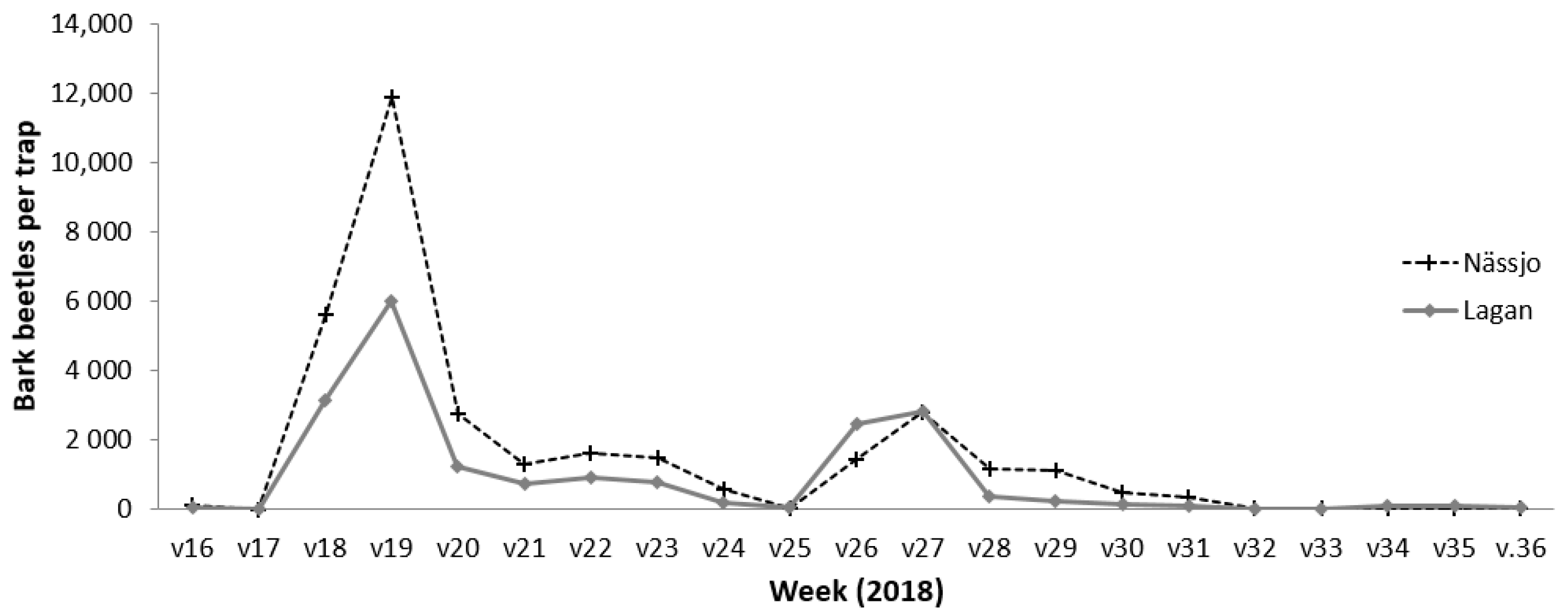
There was no information about date of attack in the harvester data. Instead, bark beetle swarming data from the Swedish forest agency were used to estimate day of attack [46]. The swarming data are based on pheromone traps that are emptied on a weekly basis during the weeks 16–36. Two stations with pheromone traps within the study area were active in 2018. The swarming activity was similar at the two stations, with a strong peak in number of trapped beetles in week 19 (second week of May), followed by six weeks with very low activity and then an increased swarming activity in the weeks 26–27, even though much lower than in week 19 (Appendix A). Hence, it is likely that most of the attacked trees in the study area were attacked around mid-May 2018.

2.2.4. Bark Beetle Risk Map

The risk map was created by Müller et al. [9] to study the variation in predisposition risk to bark beetle attacks over a 48,600 km2 study area in south Sweden, with a spatial resolution of 10 × 10 m. To identify predisposed stands, they conducted a literature review to identify environmental factors affecting the risk of attack. Then open geospatial data, acting as proxies for those factors, were downloaded, including information on local forest stand attributes (e.g., canopy height and volume spruce), topography, soil type, wetness, and the proximity of recently clear-cut areas. Positions of trees killed by bark beetles were derived from harvester machines, and random forest models were trained to classify pixels as healthy or attacked. The probability of belonging to the attacked class was considered as quantitative information of the risk of attack and used as risk map in the current study. For details, see [9].

2.3. Bark Beetle Attack Detection with Random Forest

Random forest machine learning models [47] were trained to classify pixels into attacked and healthy. For each date and tile with a sufficient amount of cloud-free data, random forest models for four scenarios were trained (Figure 2):
  • models including only data from a single date (RFdate)
  • models with only temporal features (RFtemp)
  • models including both single-date and temporal features (RFcomb)
  • models that in addition to single-date and temporal features also include the risk map (RFrisk)
The single-date models (RFdate) were trained on data from both 2017 and 2018. The temporal models (RFtemp) were trained for 2018 only since they are included with the assumption that they capture the change from before the attack (2017) to after the attack (May 2018). The number of models with temporal features included is lower than that of the single-date models since the temporal models require Sentinel-2 data with 1 year ± 2 weeks time difference (Table 1). The models with the risk map included (RFrisk) were trained to study whether, and how much, the accuracy is improved by including a risk map as a feature in the model. The single-date and temporal models were trained both with and without including the variability metrics, to study how variability influenced detection accuracy.

2.3.1. Sentinel-2-Derived Features for the Random Forest Models

Features for the random forest models were derived from Sentinel-2 data as individual pixel values for different wavelength bands, both as single-date values for the single-date models, and as the 1-year difference in pixel values for the temporal models. In addition, variability metrics were calculated and the risk map was included, which resulted in the number of features per scenario given in Table 1. The features are described in detail below.
  • Wavelength bands
All Sentinel-2 wavelength bands with 10 × 10 m and 20 × 20 m spatial resolution, except for the narrow NIR band (band 8a), were used; namely the blue (band 2), green (band 3), red (band 4), 3 × red-edge (bands 5–7), near infrared (NIR; band 8), and 2 × shortwave infrared (SWIR; bands 11–12). The 20 × 20 m bands were resampled to 10 × 10 m with nearest neighbor interpolation.
  • Variability metrics
Olsson et al. [20] showed that the variability between pixels (coefficient of variation) in a smaller window (3 × 3 pixels) can improve detection accuracy in areas with scattered bark beetle attacks. In this study, we calculated a variability metric based on squared differences according to Equation (1).
m = d i f f 1 2 + d i f f 2 2 + + d i f f n 2 ,
where diffi is the difference between the center pixel in a window and pixel i, and n is the number of pixels in the window with the same landcover as the center pixel. In this study, a window size of 3 × 3 pixels was used. Note that only pixels with the same landcover as the central pixel were included when calculating the variability metrics to avoid influence on variability due to different landcover types. This means that n is different for different locations of the 3 × 3 windows (cf. [20] where only windows where all nine pixels had the same landcover were included). The variability metric was calculated for the blue, green, red, and NIR wavelength bands, i.e., all bands with 10 × 10 m spatial resolution.
  • Temporal features
Temporal features were calculated as the 1-year difference between 2017 and 2018 (Equation (2)).
O n e _ y e a r _ d i f f b a n d = b a n d 2017 b a n d 2018
where one_year_diffband is the 1-year difference for wavelength band band; and band2017 and band2018 are reflectance for the wavelength band in 2017 and 2018, respectively. To avoid influence of phenology, a tolerance of ±2 weeks was used when calculating the difference, resulting in six images per tile. For images with a longer or shorter time difference, no temporal features were calculated. The 1-year difference was calculated for both the individual wavelength bands and the variability metrics.

2.3.2. Random Forest

The Python implementation of random forest in Scikit-learn version 1.3.0 [48] was used with default settings except for number of trees (n_estimator), which was set to 200 by prior knowledge. No tuning of hyper-parameters was done, since the main aim was to compare feature importance and accuracy between dates rather than maximizing accuracy for each single date. The random forest models were trained for dates with less than 10% of the bark-beetle-attacked pixels with no data. All pixels with no data were excluded before training the models, and the data were split into 70% training data and 30% test data, resulting in around 2400 pixels per class and tile as training data.
The random forest models were evaluated based on overall accuracy, which is the fraction of correctly classified pixels over all pixels. In this study, we refer to overall accuracy simply as accuracy; since the data set is balanced, accuracy is a reliable performance metric.
In addition, feature importance was estimated for the features in the random forest models with permutation techniques; these work by randomly permuting the values of a single feature and observing how the model’s performance changes [49]. If the model’s accuracy drops significantly, the feature is important; if the accuracy remains unaffected, the feature is less relevant. Since permutation feature importance measures the impact of shuffling individual features, it helps isolate each feature’s contribution more independently, thereby eliminating multicollinearity between features and reducing bias caused by correlated variables.

3. Results

Random forest models were trained for dates with less than 10% pixels with no data, which means that the number of random forest models differ between FORCE tiles (Table 2). For most of the dates included, there were less than 2% pixels with no data. Note that for the temporal features, the same Sentinel-2 image from 2017 can be included to calculate the 1-year difference with more than one image from 2018 since there is a ±2 weeks tolerance. This results in a higher number of 1-year-difference models in 2018 than single-date models in 2017.

3.1. Detection Accuracy for Single-Date (RFdate) and Temporal (RFtemp) Models

For the single-date random forest models, there is no trend in accuracy over the time-series (Figure 3). Accuracies are lower for Tile A, ranging from 63% to 79%, and vary considerably between dates (Figure 3a). For Tile B, the accuracies are higher, ranging from 84% to 94% (Figure 3b). For both tiles, the accuracies are high already in 2017, i.e., the year before the trees were attacked, suggesting that the influence of predisposed trees is as strong in the Sentinel-2 data as the early signs of bark-beetle-attacked trees. However, for Tile B, there is an increase in accuracy in early June 2018 compared to May the same year, which might be attributed to the bark beetle attack even if accuracies were on the same level already in 2017. It should also be noted that the last date with a sufficient number of cloud-free pixels was July 8 for Tile A, and for Tile B there were only two dates with available data in July and August.
For the random forest models with temporal features, the accuracy is also highest for Tile B, ranging from 81% to 92% (Figure 4b). Accuracy is highest before the swarming and stays stable after swarming. For Tile A, accuracies range from 65% to 81% with peaks in accuracy for May 9, which is before the swarming in the second week of May (red dashed lines), and June 1 (Figure 4a). For Tile A, the last date with a sufficient number of cloud-free pixels was July 6, and for Tile B the last date was June 8, only around three weeks after the swarming.

3.2. Detection Accuracy with Single-Date and Temporal Features Combined (RFcomb)

When both single-date and temporal features are used in the random forest model, the accuracies increase (Figure 5 and Table 3). For Tile A, accuracy ranges from 70% to 84%. The mean increase in accuracy compared to single-date models is 5.9%, with a maximum increase of 14.9%, and for the temporal models, the accuracy increases on average by 5.0%, with a maximum increase of 8.7%. For Tile B, accuracy ranges from 90% to 96%. The mean increase in accuracy compared to single-date models is 4.6%, with the maximum increase of 8.8%, and for the temporal models, the accuracy increases by on average 5.9%, with a maximum increase of 10.7%. However, since the temporal features require a Sentinel-2 image obtained one year ± 2 weeks back in time, there are fewer dates with temporal features available compared to the single-date features.

3.3. Detection Accuracy with and Without the Variability Metrics

The single-date and temporal random forest models were trained both with and without the variability metric to study how variability influences detection accuracy. For the single-date models, the variability metric increases accuracy but the increase is low, with the largest difference for dates with lower accuracy (Figure 6 and Table 4). For Tile A, the average increase when including variability is 0.8%, with a maximum increase of 5.1% (Figure 6a). For Tile B, the average increase in accuracy when including variability in the single-date models is 0.8%, with a maximum increase of 3.6% (Figure 6b).
For the temporal random forest models, there is little influence of the variability metrics on accuracy. For Tile A, the average increase in accuracy when including variability is 0.8%, with a maximum increase of 1.7% (Figure 7a). For Tile B, the average increase in accuracy is 0.5%, with a maximum increase of 1.0% (Figure 7b).

3.4. Detection Accuracy with the Risk Map Included

Including the risk map in the single-date random forest models increases accuracy for both tiles (Figure 8 and Table 5). The largest increase is for Tile A, which had lower accuracy with Sentinel-2 data alone. For the single-date models, the accuracy increases by on average 12.0%, with a highest increase of 18.1%, resulting in accuracy ranging from 81% to 88% (Figure 8a). For Tile B, with high accuracy already from the Sentinel-2 data alone, the accuracy ranges from 86% to 95% with the risk map included. The increase in accuracy is on average 1.8%, with a largest increase of 3.7% (Figure 8b). As a reference, the risk map alone was used to classify pixels into attacked and healthy based on a threshold which resulted in an accuracy of around 75% for both tiles.
Adding the risk map results in higher accuracy also for the random forest models where the single-date and temporal features are combined (Figure 9 and Table 5). For Tile A, the risk map increases accuracy by on average 8.7%, with highest increase of 13.7%, compared to the combined models resulting in accuracies ranging from 83% to 91% (Figure 9a). For Tile B, with high accuracy from the Sentinel-2 data alone, the influence of the risk map is low. The highest increase in accuracy is 2.3%, and the average increase 0.9%, resulting in accuracies ranging from 92% to 97% (Figure 9b).

3.5. Analysis of Feature Importance

Feature importance for all random forest models and all four scenarios was studied. In the figures below, the labels listed in Table 6 are used for the features. Only some of the feature importance figures are included in the results. See Supplementary Materials for feature importance from all dates.

3.5.1. Feature Importance for Single-Date Random Forest Models

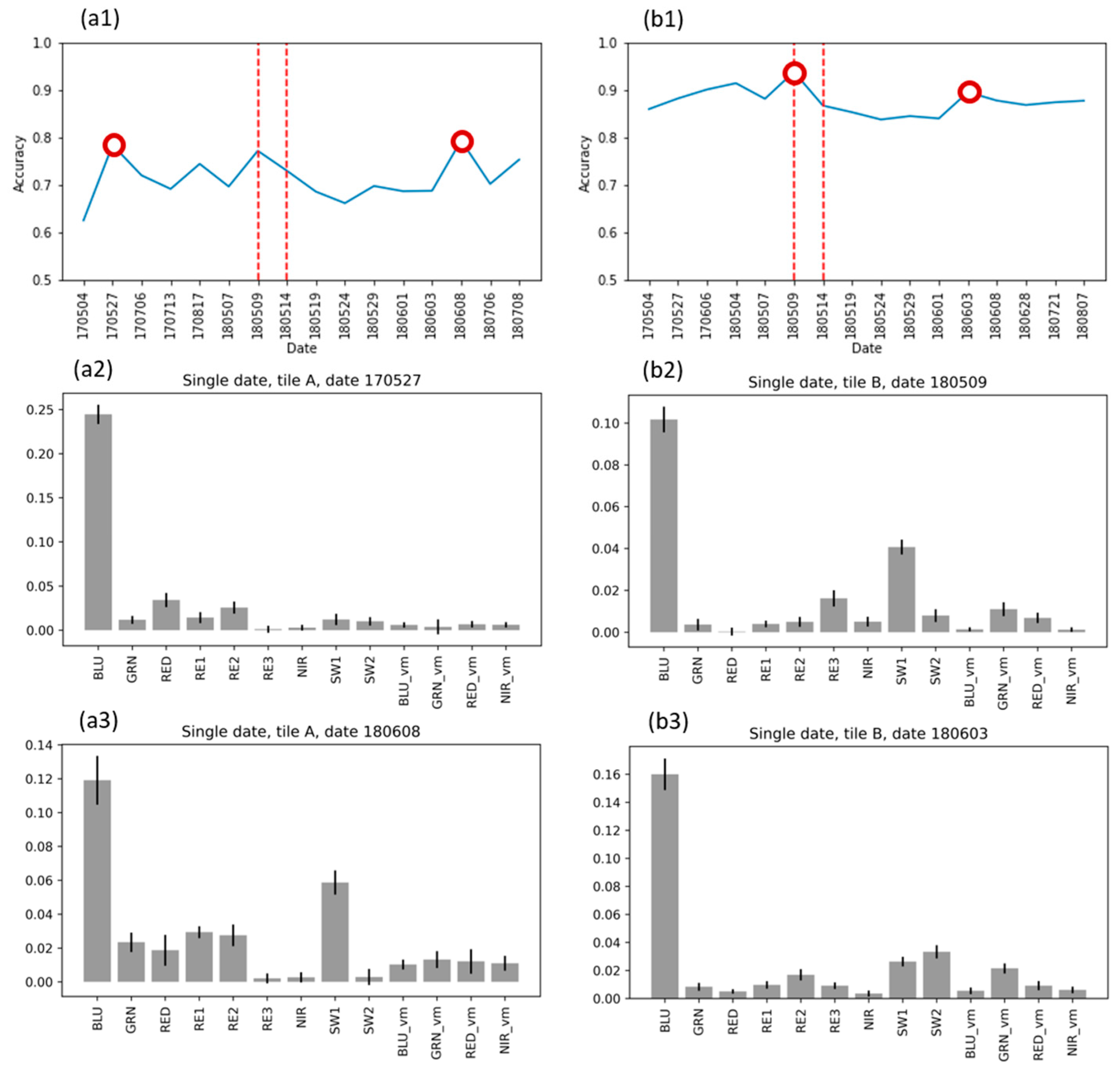
Some pattern in feature importance can be found in the time-series of single-date random forest models. For the dates with small peaks in accuracy, the blue band stands out as the most important band (Figure 10). Figure 10(a1) shows accuracy for single-date models for Tile A, with two peaks in accuracy marked (red circles), and Figure 10(a2,a3) shows feature importance for those peaks with the blue band as the most important. Figure 10(b1–b3) show two peaks in accuracy where the blue band stands out as most important for Tile B. For Tile A, the blue and the red-edge bands are generally most important for the singe-date models, followed by SWIR and the red band. For Tile B, the SWIR and red-edge bands are generally most important, followed by the blue band and the variability metric for the green band. When looking at the temporal development, the SWIR bands are more important in the later part of the time-series, i.e., after the bark beetle swarming, indicating that the SWIR bands capture the early signals from the bark beetle attack best. See Figure 11 for the last four dates with sufficient cloud-free pixels for Tile B as an example and Supplementary Materials for all dates.

3.5.2. Feature Importance for Temporal Random Forest Models

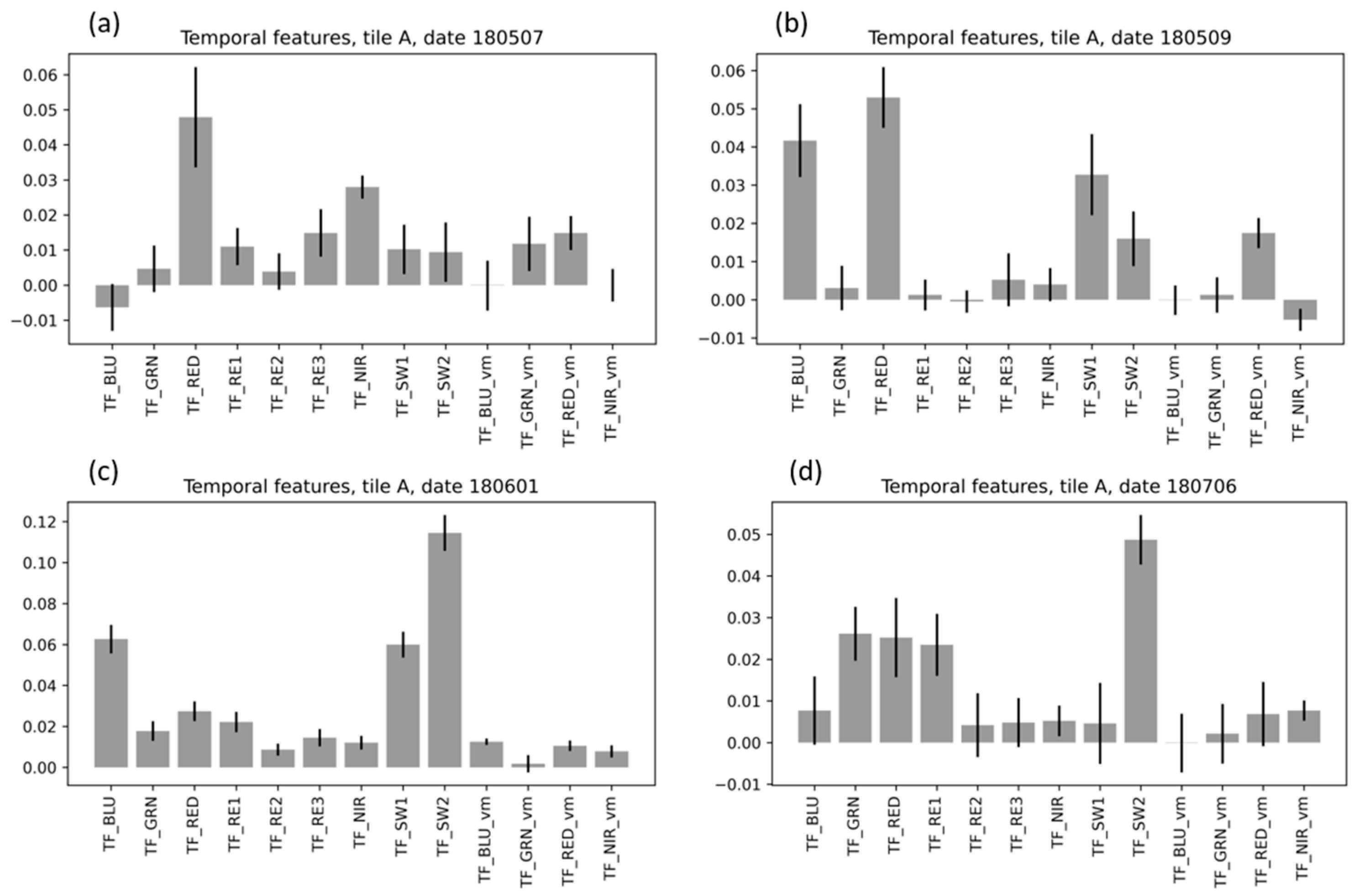
For the temporal random forest models, the most important bands in Tile A are the SWIR, red, and blue wavelength bands. For Tile B, SWIR and blue are the most important wavelength bands, followed by the red-edge and red bands. As for the single-date random forest models, the SWIR bands are generally more important in the later part of the time-series. For Tile A, the red band is the most important band for the first two dates in the time-series, while the SWIR bands are most important for the last two dates (Figure 12). See Supplementary Materials for feature importance for all dates.

3.5.3. Feature Importance for the Combined Random Forest Models

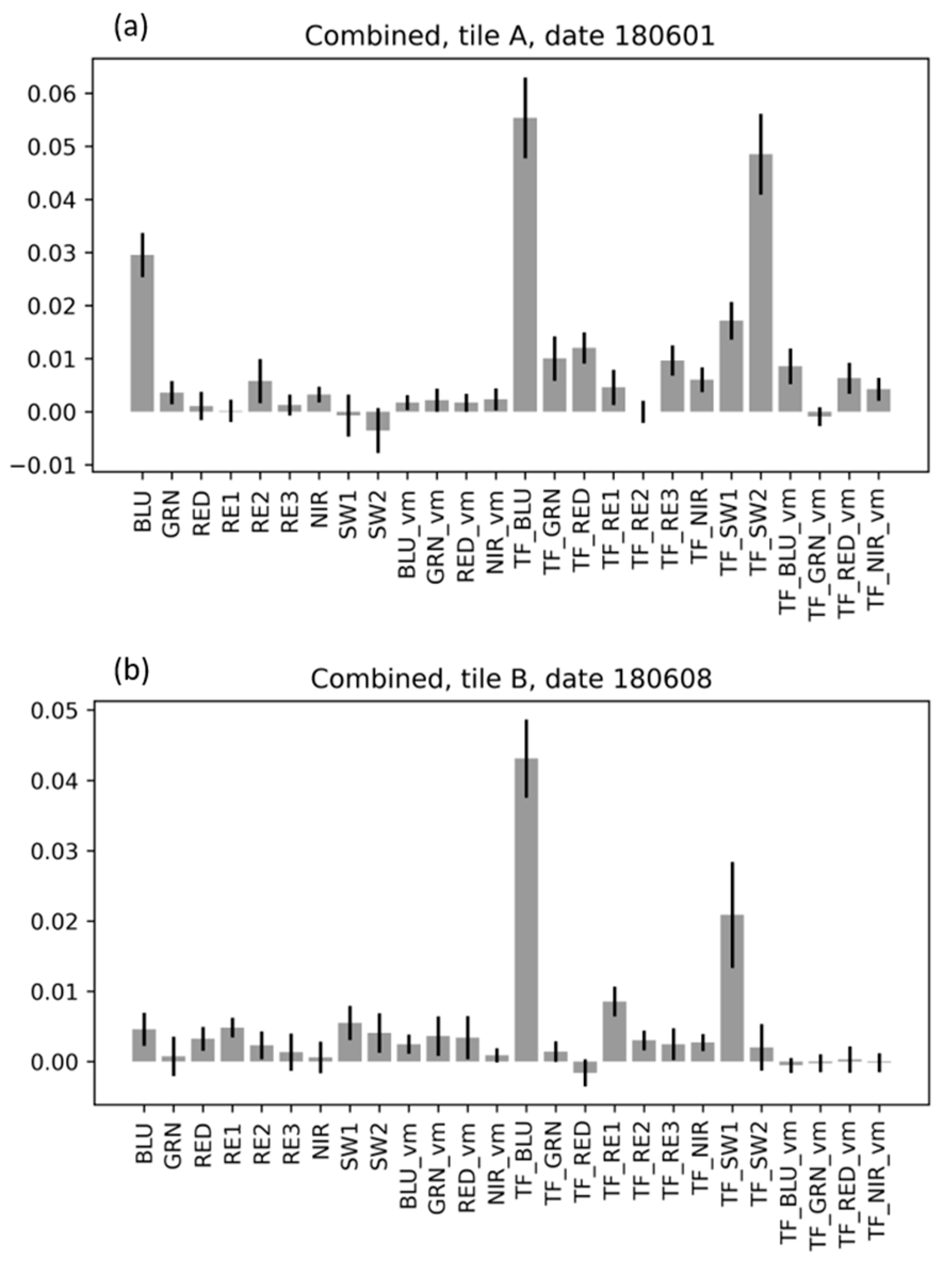
For the combined random forest models, the temporal features had overall higher importance compared with the single-date features, with the 1-year difference for the blue band as the most important feature. See Figure 13 for two examples and Supplementary Materials for feature importance for all dates.

3.5.4. Feature Importance for the Variability Metrics and Risk Map

For the single-date random forest models, the variability metrics for Tile A generally have low feature importance, with the variability metrics for the green and NIR bands as the most important. For Tile B, the variability metrics have higher importance, with the green band as the most important; for two dates, the variability of the green band is the most important feature in the single-date model. See Figure 14 for two examples and Supplementary Materials for feature importance for all dates.
For the temporal random forest models, the variability features have low importance for both tiles, with the red variability metric as the most important.
For the random forest models that included the risk map, the risk feature was by far the most important feature in Tile A for all dates, which was expected since the risk map had a strong influence on the accuracy. For Tile B, where the accuracy was high without the risk map, the risk map was the most important feature on some dates but of the same magnitude as the other features. See Supplementary Materials.

4. Discussion

This study shows that random forest models can be trained to classify Sentinel-2 pixels into the classes “predisposed and attacked” and “healthy” with high accuracies. However, the accuracies were high already before the bark beetle swarming in mid-May 2018, indicating that the models were detecting predisposed spruce trees that were later attacked, rather than attacked trees in the early stages of the attack, i.e., the detection is more related to risk of attack than actual attack. This agrees with several earlier studies [14,15,18,22]. It should, however, be noted that there were few dates with sufficient numbers of cloud-free pixels in the later part of the period studied. For the single-date models, the last date with a sufficient number of cloud-free pixels in 2018 was July 8 for Tile A and August 7 for Tile B. For the temporal models, the last date with a sufficient number of cloud-free pixels was July 6 for Tile A and June 8 for Tile B. With longer time-series, where the later stages of the attack were also included, there might have been an increase in detection accuracy, but that would be too late for early detection. It should also be noted that there are no data about date of attack available, but the swarming data (Appendix A) show a distinct peak in mid-May and low activities after that, indicating that the trees were most likely attacked in mid-May.
When single-date and temporal features were combined, the accuracy increased for both tiles. However, the single-date and temporal features can only be combined on dates with 1-year-difference data available, resulting in lower temporal resolution compared to the single-date models. An alternative to increasing the number of dates with temporal features is to allow for a longer tolerance than ±2 weeks, but that would increase the risk that phenological differences influence the 1-year difference. Consequently, the combined models result in higher accuracy, but the single-date models can be applied with higher temporal resolution. However, since the models detect predisposed trees rather than attacked trees, in the early stages a high temporal resolution is of less importance.
Earlier studies have shown that the coefficient of variation alone can be used for detection of bark-beetle-attacked trees with 86% accuracy 6–7 weeks after attack [20,21]. The variability metric included in this study had low influence on the results, even though it did increase accuracy slightly, especially for the single-date models. This indicates that the information from the variability metric added little information compared to using reflectance alone. However, a major difference between the variability metric in this study compared to the method applied in [20,21] is that in those studies, only windows where all 3 × 3 pixels had the same landcover were included. In this study, the variability metric was calculated for all windows, but only including the pixels with the same landcover as the center pixel in the calculation. If the variability is calculated from a lower number of pixels, it is likely that it will be less robust, but setting a requirement that all pixels in the window must have the same landcover would mean that the variability metrics would not be possible to calculate for a large number of windows. We did not study in what situations the variability metric performed better, e.g., whether it was in areas with more scattered trees that were attacked. However, since the accuracies were high already before the attack, the information provided by the variability metric seems to be related to predisposed trees or forest structure rather than attacked trees in the early stages.
The red-edge and SWIR bands were not included as variability metrics, even though they were important features in the random forest models and have been identified as important bands in several earlier studies [22]. The motivation for excluding those bands as variability metrics is that with a 30 × 30 m moving window applied to derive the variability metrics, there would not be much variability since the red-edge and SWIR bands have a spatial resolution of 20 × 20 m (even though they were resampled to 10 × 10 m in this study). An alternative would be to extend the size of the moving window, but then there would be fewer pixels with the same landcover in many windows; hence, we decided to calculate the variability metrics only for Sentinel-2 bands with 10 × 10 m spatial resolution.
This study indicates that the blue band is important for detection of predisposed and bark-beetle-attacked trees. Other studies have showed that the blue band is one of the least important bands for detection of bark beetle attacks [16,22]. There are, however, studies that found the blue band to be important for attack detection [18,50,51]. The blue band has also performed well for drought detection, which is likely due to the environmental stresses that influence the carotenoid levels of the needles [52]. The SWIR bands also stand out as important wavelength bands, especially for Tile B, with higher detection accuracies, and in the combined model where the temporal SWIR-features generally have high importance. Furthermore, the SWIR bands are generally more important in the later part of the time-series of random forest models, indicating that they are sensitive to the early signals of the bark beetle attack, which agrees with several other studies [15,16,18,22,53,54]. The red-edge bands are also among the most important bands for some dates, which also agrees with other studies [14,16,18,22,53,55].
The red band has been reported as one of the most important wavelength bands in some studies [15,16,22,55]. In our study, the red band has low importance for the single-date models, but for the temporal models, the red band is one of the more important bands for some dates, especially in May, both before and after swarming. A few studies have found the green band to be important for detection of bark beetle attacks [22,55,56]. In this study, the green band has low feature importance for the single-date and temporal models, but the green band is one of the more important variability metrics, and for some dates the green variability metric is the most important feature.
There were no trends in feature importance over time except for the SWIR bands that were more important after bark beetle swarming. However, the blue band had generally high importance for dates when the random forest models achieved high accuracy, which might be related to atmospheric conditions, since the blue band is more sensitive to atmospheric disturbance (e.g., scattering due to aerosols, etc.) and has a low signal-to-noise ratio compared to longer wavelength bands [57]. This could potentially explain the variability in accuracy with time, even though the Sentinel-2 data were atmospherically corrected. In conditions with low atmospheric disturbances, there is less noise in the blue band, which could result in higher detection accuracy, while the accuracy is lower for dates with more atmospheric disturbances when the blue band includes more noise.
Earlier studies have included vegetation indices for detection of bark-beetle-attacked trees [13,14,15,16,17,18,19,20,21,22]. In this study, we only include individual wavelength bands, since we wanted to study which wavelength bands are more important for monitoring predisposed and attacked trees and whether the importance of the wavelength bands changes with time after attack. If we had included vegetations indices, it would be more difficult to interpret the results.
In this study, we excluded all dates with more than 10% cloud cover for the pixels with bark beetle damage data. There could be sufficient data to train random forest models also for dates with higher cloud cover to obtain a denser time-series, but then it is likely that the cloud-free data for different dates are from different parts of the FORCE tiles, and the models might not be directly comparable due to spatial differences within the tiles. Since the focus is to study how accuracy changed with time after bark beetle swarming, the spatial differences should be kept low. It would also be possible to merge the two tiles to retrieve more data and train random forest models for additional dates, but then spatial differences in the study area would have a larger influence on the models. The differences in accuracies, as well as feature importance, between the tiles suggest that there are differences between them and that the tiles should be handled separately. To the best of the authors’ knowledge, no studies have been performed in which the different parts of the study have been treated differently, and most studies are performed on relatively small areas [22].
The high detection accuracies already achieved before the bark beetle swarming suggests that the Sentinel-2 data identify trees at high risk of attack rather than attacked trees. Furthermore, no trends with increasing accuracies were found after the bark beetle swarming as anticipated, indicating that there are limitations in the ability to detect attacked trees at the early stages. However, the increased accuracy when combining the Sentinel-2 data with the static risk map created with forestry data and geodata demonstrates how remote sensing data and geodata can be combined to improve and update risk maps. Such risk maps can be valuable tools to guide forest managers in searching for attacked trees in areas with elevated risk of bark beetle attack [22].
In addition, the results show how single-date and temporal features can be combined to increase accuracy, and that the spatial domain can be included by adding variability features. An interesting way forward would be to apply convolutional machine learning models; since convolutional models apply kernels covering several pixels in a small sliding window, they should be able to capture the spatial domain. Another alternative is to establish the baseline conditions for a pixel, accounting for the phenology over the growing season, and compare new observations with the baseline [14,58]. However, that requires some years of data prior to the attack to estimate the baseline conditions.
The different results for the two tiles also show that there are differences in how well the predisposed and attacked trees can be detected. To obtain an indication of potential causes of the differences in accuracy, we checked whether there were differences in forest types and forest attributes between the two tiles based on the features used to create the risk map in [9]. For both tiles, the attacked pixels were located in the same forest types, with similar forestry attributes (canopy height, spruce volume, and basal area) and with similar topography, suggesting that there are other reasons for the differences in accuracy. This suggests that geographically weighted methods, such as geographically weighted random forest [59], should be applied to detect attacked trees and for risk mapping. With geographically weighted methods, spatial autocorrelation is explored and a number of local models are trained instead of one global model, but to develop such models, large data sets over large areas are required.

5. Conclusions

The random forest models trained in this study could detect Sentinel-2 pixels with predisposed and bark-beetle-attacked trees with high accuracy, but detection accuracy did not increase with time after bark beetle swarming. This suggests that the models detect weakened trees, that were later attacked, with similar accuracy as attacked trees in the early stages.
The single-date and temporal (1-year difference) random forest models resulted in similar accuracies. When both single-date Sentinel-2 data and temporal features were included in the random forest models, the accuracy increased by around 5%. However, since the temporal features require data from one year earlier, the temporal resolution of the temporal and combined random forest models is lower compared to models that only require single-date Sentinel-2 images. Including variability in the random forest models only slightly increased accuracy.
In this study, the blue, SWIR, and red-edge bands were the most important wavelength bands, with the SWIR bands being more important after bark beetle swarming, indicating that they are the most suitable bands for early detection of bark beetle attacks. For the temporal features, the red band is one of the more important features, and the green band is the most important band when looking at the variability features. When a risk map is included in the random forest models, the accuracy increases, with the strongest increase where accuracy is low from Sentinel-2 data alone.
Accuracy as well as feature importance differed between the two tiles, suggesting that there are local differences and that geographically weighted methods should be applied for detection of predisposed and bark-beetle-attacked trees. A way forward would be to apply geographically weighted methods where Sentinel-2 data and risk maps are combined, but where the risk maps are updated frequently to have a more dynamic monitoring system for trees predisposed to and attacked by bark beetles to support forest management.

Supplementary Materials

The following supporting information can be downloaded at: https://www.mdpi.com/article/10.3390/rs16224166/s1, Feature importance figures from the random forest models for all dates.

Author Contributions

Conceptualization, P.-O.O., P.Z. and A.M.; methodology, P.-O.O. and P.Z.; software, P.-O.O. and P.Z.; formal analysis, P.-O.O. and P.Z.; investigation, P.-O.O. and P.Z.; resources, J.A.; data curation, P.-O.O. and M.M.; writing—original draft preparation, P.-O.O.; writing—review and editing, all authors; visualization, P.-O.O.; project administration, P.-O.O.; funding acquisition, P.-O.O. All authors have read and agreed to the published version of the manuscript.

Funding

This research was funded by the Swedish National Space Agency, grant Dnr. 2020-00173.

Data Availability Statement

The authors do not have permission to share the bark beetle data. The risk maps can be shared upon request as well as the data used to create the risk maps.

Acknowledgments

This study was funded by the Swedish National Space Agency (Grant Dnr. 2020-00173). MM was supported by the Swedish research area BECC (Biodiversity and Ecosystem services in a Changing Climate). The authors acknowledge Sveaskog, the largest forest owner in Sweden, and the forest owner association Södra for providing harvester data, and the Swedish Forest Agency (Skogsstyrelsen) and the National Forest Inventory (NFI) for providing bark beetle presence data. They thank the Center for Scientific and Technical Computing at Lund University (LUNARC) for proving resources of computation and storage within the Swedish National Infrastructure for Computing project (LU 2022/2-14; PI Jonas Ardö).

Conflicts of Interest

The authors declare no conflicts of interest.

Appendix A

Figure A1. Bark beetle swarming data at the two stations inside (Nässjö) and just outside (Lagan) the study area. The data show the number of bark beetles caught in pheromone traps on a weekly basis. For both stations, the main swarming is in week 19 (second week of May), with high numbers of beetles also in week 18.
Remotesensing 16 04166 g0a1

References

  1. Patacca, M.; Lindner, M.; Lucas-Borja, M.E.; Cordonnier, T.; Fidej, G.; Gardiner, B.; Hauf, Y.; Jasinevičius, G.; Labonne, S.; Linkevičius, E.; et al. Significant increase in natural disturbance impacts on European forests since 1950. Glob. Chang. Biol. 2023, 29, 1359–1376. [Google Scholar] [CrossRef] [PubMed]
  2. Schelhaas, M.-J.; Nabuurs, G.-J.; Schuck, A. Natural disturbances in the European forests in the 19th and 20th centuries. Glob. Chang. Biol. 2003, 9, 1620–1633. [Google Scholar] [CrossRef]
  3. Hlásny, T.; König, L.; Krokene, P.; Lindner, M.; Montagné-Huck, C.; Müller, J.; Qin, H.; Raffa, K.F.; Schelhaas, M.-J.; Svoboda, M.; et al. Bark Beetle Outbreaks in Europe: State of Knowledge and Ways Forward for Management. Curr. For. Rep. 2021, 7, 138–165. [Google Scholar] [CrossRef]
  4. Jactel, H.; Petit, J.; Desprez-Loustau, M.-L.; Delzon, S.; Piou, D.; Battisti, A.; Koricheva, J. Drought effects on damage by forest insects and pathogens: A meta-analysis. Glob. Chang. Biol. 2012, 18, 267–276. [Google Scholar] [CrossRef]
  5. Netherer, S.; Panassiti, B.; Pennerstorfer, J.; Matthews, B. Acute Drought Is an Important Driver of Bark Beetle Infestation in Austrian Norway Spruce Stands. Front. For. Glob. Chang. 2019, 2, 39. [Google Scholar] [CrossRef]
  6. Marini, L.; Lindelöw, Å.; Jönsson, A.M.; Wulff, S.; Schroeder, L.M. Population dynamics of the spruce bark beetle: A long-term study. Oikos 2013, 122, 1768–1776. [Google Scholar] [CrossRef]
  7. Jönsson, A.M.; Schroeder, L.M.; Lagergren, F.; Anderbrant, O.; Smith, B. Guess the impact of Ips typographus—An ecosystem modelling approach for simulating spruce bark beetle outbreaks. Agric. For. Meteorol. 2012, 166–167, 188–200. [Google Scholar] [CrossRef]
  8. Bentz, B.J.; Jönsson, A.M.; Schroeder, M.; Weed, A.; Wilcke, R.A.I.; Larsson, K. Ips typographus and Dendroctonus ponderosae Models Project Thermal Suitability for Intra- and Inter-Continental Establishment in a Changing Climate. Front. For. Glob. Chang. 2019, 2, 1. [Google Scholar] [CrossRef]
  9. Müller, M.; Olsson, P.O.; Eklundh, L.; Jamali, S.; Ardö, J. Features predisposing forest to bark beetle outbreaks and their dynamics during drought. For. Ecol. Manag. 2022, 523, 120480. [Google Scholar] [CrossRef]
  10. Kärvemo, S.; Huo, L.; Öhrn, P.; Lindberg, E.; Persson, H.J. Different triggers, different stories: Bark-beetle infestation patterns after storm and drought-induced outbreaks. For. Ecol. Manag. 2023, 545, 121255. [Google Scholar] [CrossRef]
  11. Wulder, M.A.; Dymond, C.C.; White, J.C.; Leckie, D.G.; Carroll, A.L. Surveying mountain pine beetle damage of forests: A review of remote sensing opportunities. For. Ecol. Manag. 2006, 221, 27–41. [Google Scholar] [CrossRef]
  12. Senf, C.; Seidl, R.; Hostert, P. Remote sensing of forest insect disturbances: Current state and future directions. Int. J. Appl. Earth Obs. Geoinf. 2017, 60, 49–60. [Google Scholar] [CrossRef] [PubMed]
  13. Abdullah, H.; Skidmore, A.K.; Darvishzadeh, R.; Heurich, M. Sentinel-2 accurately maps green-attack stage of European spruce bark beetle (Ips typographus, L.) compared with Landsat-8. Remote Sens. Ecol. Conserv. 2018, 5, 87–106. [Google Scholar] [CrossRef]
  14. König, S.; Thonfeld, F.; Förster, M.; Dubovyk, O.; Heurich, M. Assessing Combinations of Landsat, Sentinel-2 and Sentinel-1 Time series for Detecting Bark Beetle Infestations. GIScience Remote Sens. 2023, 60, 2226515. [Google Scholar] [CrossRef]
  15. Huo, L.; Lindberg, E.; Bohlin, J.; Persson, H.J. Assessing the detectability of European spruce bark beetle green attack in multispectral drone images with high spatial- and temporal resolutions. Remote Sens. Environ. 2023, 287, 113484. [Google Scholar] [CrossRef]
  16. Bárta, V.; Lukeš, P.; Homolová, L. Early detection of bark beetle infestation in Norway spruce forests of Central Europe using Sentinel-2. Int. J. Appl. Earth Obs. Geoinf. 2021, 100, 102335. [Google Scholar] [CrossRef]
  17. Dalponte, M.; Solano-Correa, Y.T.; Frizzera, L.; Gianelle, D. Mapping a European Spruce Bark Beetle Outbreak Using Sentinel-2 Remote Sensing Data. Remote Sens. 2022, 14, 3135. [Google Scholar] [CrossRef]
  18. Candotti, A.; De Giglio, M.; Dubbini, M.; Tomelleri, E. A Sentinel-2 Based Multi-Temporal Monitoring Framework for Wind and Bark Beetle Detection and Damage Mapping. Remote Sens. 2022, 14, 6105. [Google Scholar] [CrossRef]
  19. Jamali, S.; Olsson, P.-O.; Ghorbanian, A.; Müller, M. Examining the potential for early detection of spruce bark beetle attacks using multi-temporal Sentinel-2 and harvester data. ISPRS J. Photogramm. Remote Sens. 2023, 205, 352–366. [Google Scholar] [CrossRef]
  20. Olsson, P.O.; Bergman, H.; Piltz, K. Exploring the potential to use in-between pixel variability for early detection of bark beetle attacked trees. AGILE GIScience Ser. 2023, 4, 35. [Google Scholar] [CrossRef]
  21. Jamali, S.; Olsson, P.O.; Müller, M.; Ghorbanian, A. Kernel-Based Early Detection of Forest Bark Beetle Attack Using Vegetation Indices Time Series of Sentinel-2. IEEE J. Sel. Top. Appl. Earth Obs. Remote Sens. 2024, 17, 12868–12877. [Google Scholar] [CrossRef]
  22. Kautz, M.; Feurer, J.; Adler, P. Early detection of bark beetle (Ips typographus) infestations by remote sensing—A critical review of recent research. For. Ecol. Manag. 2024, 556, 121595. [Google Scholar] [CrossRef]
  23. Lindbladh, M.; Axelsson, A.-L.; Hultberg, T.; Brunet, J.; Felton, A. From broadleaves to spruce—The borealization of southern Sweden. Scand. J. For. Res. 2014, 29, 686–696. [Google Scholar] [CrossRef]
  24. SMHI. Månads-, Årstids- och Årskartor. 2024. Available online: https://www.smhi.se/data/meteorologi/kartor/normal/arstidsmedeltemperatur-normal/sommar (accessed on 20 August 2024).
  25. Schroeder, M. Granbarkborrens Förökningsframgång i Dödade Träd Under Sommaren 2022 i Sydöstra Småland, Värmland och Uppland/Västmanland. Swedish University of Agricultural Sciences. 2023. Available online: https://www.slu.se/globalassets/ew/org/inst/ekol/rapporter/granbarkborrens-forokningsframgang-2022.pdf (accessed on 29 December 2023).
  26. Lantmäteriet. GSD-Fastighetskartan Vektor Version 7.5.5. 2021. Available online: https://www.lantmateriet.se/sv/kartor/ (accessed on 5 October 2021).
  27. OpenStreetMap Contributors. OpenStreetMap’s Standard Tile Layer. 2024. Available online: https://tile.openstreetmap.org/ (accessed on 16 April 2024).
  28. Frantz, D. FORCE—Landsat + Sentinel-2 Analysis Ready Data and Beyond. Remote Sens. 2019, 11, 1124. [Google Scholar] [CrossRef]
  29. Tanré, D.; Herman, M.; Deschamps, P.Y.; de Leffe, A. Atmospheric modeling for space measurements of ground reflectances, including bidirectional properties. Appl. Opt. 1979, 18, 3587–3594. [Google Scholar] [CrossRef]
  30. Tanré, D.; Deroo, C.; Duhaut, P.; Herman, M.; Morcrette, J.J.; Perbos, J.; Deschamps, P.Y. Technical note Description of a computer code to simulate the satellite signal in the solar spectrum: The 5S code. Int. J. Remote Sens. 1990, 11, 659–668. [Google Scholar] [CrossRef]
  31. Zhu, Z.; Wang, S.; Woodcock, C.E. Improvement and expansion of the Fmask algorithm: Cloud, cloud shadow, and snow detection for Landsats 4–7, 8, and Sentinel 2 images. Remote Sens. Environ. 2015, 159, 269–277. [Google Scholar] [CrossRef]
  32. Zhu, Z.; Woodcock, C.E. Object-based cloud and cloud shadow detection in Landsat imagery. Remote Sens. Environ. 2012, 118, 83–94. [Google Scholar] [CrossRef]
  33. Frantz, D.; Haß, E.; Uhl, A.; Stoffels, J.; Hill, J. Improvement of the Fmask algorithm for Sentinel-2 images: Separating clouds from bright surfaces based on parallax effects. Remote Remote Sens. Environ. 2018, 215, 471–481. [Google Scholar] [CrossRef]
  34. Royer, A.; Charbonneau, L.; Teillet, P.M. Interannual landsat-MSS reflectance variation in an urbanized temperate zone. Remote Sens. Environ. 1988, 24, 423–446. [Google Scholar] [CrossRef]
  35. Hill, J. High Precision Land Cover Mapping and Inventory with Multi-Temporal Earth Observation Satellite Data: The Ardèche Experiment. Ph.D. Thesis, Trier University, Trier, Germany, 1993. [Google Scholar]
  36. Sobolev, V.V.; Haar, D. Light Scattering in Planetary Atmospheres: International Series of Monographs in Natural Philosophy; Elsevier Science: Amsterdam, The Netherlands, 2017. [Google Scholar]
  37. Frantz, D.; Stellmes, M.; Hostert, P. A Global MODIS Water Vapor Database for the Operational Atmospheric Correction of Historic and Recent Landsat Imagery. Remote Sens. 2019, 11, 257. [Google Scholar] [CrossRef]
  38. Roy, D.P.; Li, J.; Zhang, H.K.; Yan, L.; Huang, H.; Li, Z. Examination of Sentinel-2A multi-spectral instrument (MSI) reflectance anisotropy and the suitability of a general method to normalize MSI reflectance to nadir BRDF adjusted reflectance. Remote Sens. Environ. 2017, 199, 25–38. [Google Scholar] [CrossRef]
  39. Roy, D.P.; Li, Z.; Zhang, H.K. Adjustment of Sentinel-2 Multi-Spectral Instrument (MSI) Red-Edge Band Reflectance to Nadir BRDF Adjusted Reflectance (NBAR) and Quantification of Red-Edge Band BRDF Effects. Remote Sens. 2017, 9, 1325. [Google Scholar] [CrossRef]
  40. Roy, D.P.; Zhang, H.K.; Ju, J.; Gomez-Dans, J.L.; Lewis, P.E.; Schaaf, C.B.; Sun, Q.; Li, J.; Huang, H.; Kovalskyy, V. A general method to normalize Landsat reflectance data to nadir BRDF adjusted reflectance. Remote Sens. Environ. 2016, 176, 255–271. [Google Scholar] [CrossRef]
  41. Rufin, P.; Frantz, D.; Yan, L.; Hostert, P. Operational Coregistration of the Sentinel-2A/B Image Archive Using Multitemporal Landsat Spectral Averages. IEEE Geosci. Remote Sens. Lett. 2021, 18, 712–716. [Google Scholar] [CrossRef]
  42. FORCE. FORCE Time Series Analysis. 2023. Available online: https://force-eo.readthedocs.io/en/latest/components/higher-level/tsa/index.html (accessed on 2 January 2024).
  43. SMHI. April 2018—Årets Första Vårmånad. 2018. Available online: https://www.smhi.se/klimat/klimatet-da-och-nu/manadens-vader-och-vatten-sverige/manadens-vader-i-sverige/april-2018-arets-forsta-varmanad-1.133032 (accessed on 3 January 2023).
  44. Naturvårdsverket. National Land Cover Database (NMD). 2021. Available online: https://www.naturvardsverket.se/en/services-and-permits/maps-and-map-services/national-land-cover-database/ (accessed on 20 August 2021).
  45. Lantmäteriet. GSD-Terrängkartan, Vektor. Version 5.10. 2021. Available online: https://www.lantmateriet.se/globalassets/geodata/geodataprodukter/produktlista/terrshmi.pdf (accessed on 5 January 2021).
  46. Skogsstyrelsen. Svarmningsövervakning. 2023. Available online: https://www.skogsstyrelsen.se/statistik/statistik-efter-amne/svarmningsovervakning/ (accessed on 20 August 2024).
  47. Breiman, L. Random Forests. Mach. Learn. 2001, 45, 5–32. [Google Scholar] [CrossRef]
  48. Pedregosa, F.; Varoquaux, G.; Gramfort, A.; Michel, V.; Thirion, B.; Grisel, O.; Blondel, M.; Prettenhofer, P.; Weiss, R.; Dubourg, V.; et al. Scikit-learn: Machine Learning in Python. J. Mach. Learn. Res. 2011, 12, 2825–2830. [Google Scholar]
  49. Altmann, A.; Toloşi, L.; Sander, O.; Lengauer, T. Permutation importance: A corrected feature importance measure. Bioinformatics 2010, 26, 1340–1347. [Google Scholar] [CrossRef]
  50. Junttila, S.; Näsi, R.; Koivumäki, N.; Imangholiloo, M.; Saarinen, N.; Raisio, J.; Holopainen, M.; Hyyppä, H.; Hyyppä, J.; Lyytikäinen-Saarenmaa, P.; et al. Multispectral Imagery Provides Benefits for Mapping Spruce Tree Decline Due to Bark Beetle Infestation When Acquired Late in the Season. Remote Sens. 2022, 14, 909. [Google Scholar] [CrossRef]
  51. Trubin, A.; Kozhoridze, G.; Zabihi, K.; Modlinger, R.; Singh, V.V.; Surový, P.; Jakuš, R. Detection of susceptible Norway spruce to bark beetle attack using PlanetScope multispectral imagery. Front. For. Glob. Chang. 2023, 6, 1130721. [Google Scholar] [CrossRef]
  52. Vicca, S.; Balzarolo, M.; Filella, I.; Granier, A.; Herbst, M.; Knohl, A.; Longdoz, B.; Mund, M.; Nagy, Z.; Pintér, K.; et al. Remotely-sensed detection of effects of extreme droughts on gross primary production. Sci. Rep. 2016, 6, 28269. [Google Scholar] [CrossRef] [PubMed]
  53. Fassnacht, F.E.; Latifi, H.; Ghosh, A.; Joshi, P.K.; Koch, B. Assessing the potential of hyperspectral imagery to map bark beetle-induced tree mortality. Remote Sens. Environ. 2014, 140, 533–548. [Google Scholar] [CrossRef]
  54. Abdullah, H.; Darvishzadeh, R.; Skidmore, A.K.; Groen, T.A.; Heurich, M. European spruce bark beetle (Ips typographus, L.) green attack affects foliar reflectance and biochemical properties. Int. J. Appl. Earth Obs. Geoinf. 2018, 64, 199–209. [Google Scholar] [CrossRef]
  55. Huo, L.; Lindberg, E.; Fransson, J.E.S.; Persson, H.J. Comparing Spectral Differences Between Healthy and Early Infested Spruce Forests Caused by Bark Beetle Attacks using Satellite Images. In Proceedings of the IGARSS 2022—2022 IEEE International Geoscience and Remote Sensing Symposium, Kuala Lumpur, Malaysia, 17–22 July 2022; pp. 7709–7712. [Google Scholar]
  56. Huo, L.; Koivumäki, N.; Oliveira, R.A.; Hakala, T.; Markelin, L.; Näsi, R.; Suomalainen, J.; Polvivaara, A.; Junttila, S.; Honkavaara, E. Bark beetle pre-emergence detection using multi-temporal hyperspectral drone images: Green shoulder indices can indicate subtle tree vitality decline. ISPRS J. Photogramm. Remote Sens. 2024, 216, 200–216. [Google Scholar] [CrossRef]
  57. Zhen, Z.; Chen, S.; Yin, T.; Gastellu-Etchegorry, J.-P. Globally quantitative analysis of the impact of atmosphere and spectral response function on 2-band enhanced vegetation index (EVI2) over Sentinel-2 and Landsat-8. ISPRS J. Photogramm. Remote Sens. 2023, 205, 206–226. [Google Scholar] [CrossRef]
  58. Olsson, P.-O.; Lindström, J.; Eklundh, L. Near real-time monitoring of insect induced defoliation in subalpine birch forests with MODIS derived NDVI. Remote Sens. Environ. 2016, 181, 42–53. [Google Scholar] [CrossRef]
  59. Georganos, S.; Grippa, T.; Niang Gadiaga, A.; Linard, C.; Lennert, M.; Vanhuysse, S.; Mboga, N.; Wolff, E.; Kalogirou, S. Geographical random forests: A spatial extension of the random forest algorithm to address spatial heterogeneity in remote sensing and population modelling. Geocarto Int. 2021, 36, 121–136. [Google Scholar] [CrossRef]
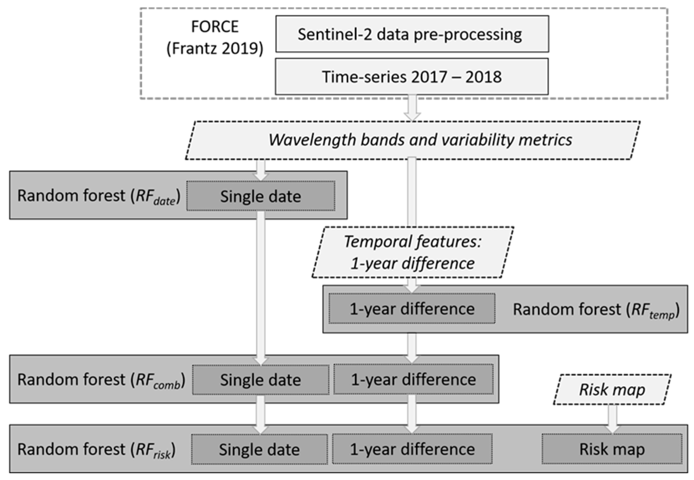
Figure 2. The random forest models for four scenarios that were trained for each date and tile with sufficient number of cloud-free pixels. The single-date and temporal models were trained both with and without the variability metrics.
Remotesensing 16 04166 g002
Figure 3. Accuracy of the random forest models with single-date features for Tile A (a) and Tile B (b). The main swarming week is between the red dashed lines.
Remotesensing 16 04166 g003
Figure 4. Accuracy of the random forest models with temporal (1-year difference) features for Tile A (a) and Tile B (b). The main swarming week is between the red dashed lines.
Remotesensing 16 04166 g004
Figure 5. Accuracy of the random forest models with single-date features only (blue), temporal (1-year difference) features only (green), and both combined (black) for Tile A (a) and Tile B (b). The main swarming week is between the red dashed lines.
Remotesensing 16 04166 g005
Figure 6. Accuracy of the single-date random forest models with and without variability metrics for Tile A (a) and Tile B (b). The main swarming week is between the red dashed lines.
Remotesensing 16 04166 g006
Figure 7. Accuracy of the temporal random forest models with and without variability metrics for Tile A (a) and Tile B (b). The main swarming week is between the red dashed lines.
Remotesensing 16 04166 g007
Figure 8. Accuracy of the single-date random forest models with (blue dotted) and without (solid blue) the risk map for Tile A (a) and Tile B (b). The main swarming week is between the red dashed lines.
Remotesensing 16 04166 g008
Figure 9. Accuracy of the random forest models with single-date and temporal features combined (black) and accuracy when risk is added as a feature (black dotted) for Tile A (a) and Tile B (b). Accuracies for models with single-date (blue) and temporal (green) features are included as reference. The main swarming week is between the red dashed lines.
Remotesensing 16 04166 g009
Figure 10. Accuracy of the single-date random forest (RFdate) models for Tile A (a1a3) and Tile B (b1b3) with four examples of peaks in accuracy (red circle). At the peaks with higher accuracy, the blue band stands out as the most important (a2b3). Note that (a2,b2) are from before the main swarming in 2018 and related to predisposed trees rather than bark beetle attack. See Table 6 for feature labels and Supplementary Materials for feature importance for all dates.
Remotesensing 16 04166 g010
Figure 11. Feature importance for the single-date random forest model (RFdate) for the last four dates with sufficient number of cloud-free pixels in Tile B. For all dates, the SWIR bands stands out as highly important features. See Supplementary Materials for feature importance for all dates where the SWIR bands are generally less important for the earlier dates, and Table 6 for band labels.
Remotesensing 16 04166 g011
Figure 12. Feature importance for the temporal random forest models (RFtemp) for Tile A. The red band is the most important wavelength band for the first two dates (a,b), and the SWIR bands are most important for the last two dates (c,d). See Table 6 for feature labels and Supplementary Materials for all dates.
Remotesensing 16 04166 g012
Figure 13. Feature importance for the combined random forest models (RFcomb) for Tile A (a) and Tile B (b) for one date each when the 1-year difference for the blue band is the most important feature. See Table 6 for feature labels and Supplementary Materials for feature importance for all dates.
Remotesensing 16 04166 g013
Figure 14. Feature importance for single-date random forest models (RFdate) for Tile B and dates when the variability metric for the green band is the most important feature. For both dates, accuracy is relatively low (Figure 3b). See Table 6 for feature labels and Supplementary Materials for feature importance for all dates.
Remotesensing 16 04166 g014
Table 1. The number of features in the random forest models for the four scenarios. RFdate models include single-date Sentinel-2 data and variability metrics. RFtemp models include temporal (1-year difference) data and variability metrics derived from 1-year difference. RFcomb includes single-date and 1-year-difference data as well as variability metrics. RFrisk includes the risk map in addition to the data used in the RFcomb model.
Number of Features
Random Forest ModelSingle Date1-Year DifferenceVariabilityRiskTotal
Single date (RFdate)9 4 13
1-year diff. (RFtemp) 94 13
Combined (RFcomb)998 26
Risk (RFrisk)998127
Table 2. The number of random forest (RF) models per FORCE tile and year. The same single date model in 2017 can be included in more than one 1-year-difference model in 2018.
Number of RF Models 2017Number of RF Models 2018
TileSingle DateSingle Date1-Year Difference
A (north)5116
B (south)313 6
Table 3. Increase in accuracy of the random forest models with single-date and temporal features combined.
Combined—Single DateCombined—Temporal
TileMean Diff.Max Diff.Mean Diff.Max Diff.
Tile A (north)5.9%14.9%4.6%8.8%
Tile B (south)5.0%8.7%5.9%10.7%
Table 4. Increase in accuracy of the single-date and temporal random forest models when the variability metric is included.
Single-Date ModelsTemporal Models
TileMean Diff.Max Diff.Mean Diff.Max Diff.
Tile A (north)0.8%5.1%0.8%1.7%
Tile B (south)0.8%3.6%0.5%1.0%
Table 5. Increase in accuracy of the random forest models when the risk map is included as a feature in the random forest models.
Single-Date ModelsCombined Models
TileMean Diff.Max Diff.Mean Diff.Max Diff.
Tile A (north)12.0%18.1%8.7%13.7%
Tile B (south)1.8%3.7%0.9%2.3%
Table 6. Sentinel-2 wavelength bands included in the random forest models with the labels used for the features in the figures below. TF_ is used as a prefix for temporal features and _vm is used as a suffix for the spatial variability metrics.
Feature Labels
Spatial Variability Metrics
Sentinel-2 BandResolution
(m)
Single Date1-Year Diff.Single Date1-Year Diff.
Band 2, Blue10BLUTF_BLUBLU_vmTF_BLU_vm
Band 3, Green10GRNTF_GRNGRN_vmTF_GRN_vm
Band 4, Red10REDTF_REDRED_vmTF_RED_vm
Band 5, red-edge120RE1TF_RE1
Band 6, red-edge220RE2TF_RE2
Band 7, red-edge320RE3TF_RE3
Band 8, NIR10NIRTF_NIRNIR_vmTF_NIR_vm
Band 11, SWIR120SW1TF_SW1
Band 12, SWIR220SW2TF_SW2
Disclaimer/Publisher’s Note: The statements, opinions and data contained in all publications are solely those of the individual author(s) and contributor(s) and not of MDPI and/or the editor(s). MDPI and/or the editor(s) disclaim responsibility for any injury to people or property resulting from any ideas, methods, instructions or products referred to in the content.