Article

The Spatiotemporal Evolution of the Mudflat Wetland in the Yellow Sea Using Landsat Time Series

1
Land Science Research Center, Nanjing University of Information Science and Technology, Nanjing 210044, China
2
Hebei Meteorological Technology and Equipment Center, Shijiazhuang 050022, China
3
Department of Civil and Architectural Engineering and Construction Management, University of Wyoming, Laramie, WY 82071, USA
*
Author to whom correspondence should be addressed.
Remote Sens. 2024, 16(22), 4190; https://doi.org/10.3390/rs16224190
Submission received: 5 September 2024 / Revised: 22 October 2024 / Accepted: 7 November 2024 / Published: 10 November 2024
(This article belongs to the Section Remote Sensing in Geology, Geomorphology and Hydrology)

Abstract

:
Mudflat wetland, one of the 27 surface elements identified by the International Geographic Data Committee, has undergone substantial transformations with the rapid growth of the social economy and marine hazards, resulting in significant changes in its area and distribution. Quick identification of mudflat wetland evolution is vital to improve the mudflat ecological service value. We employed object-oriented and decision tree classification methods to map the mudflat wetland in the Yellow Sea using the Landsat time series from 1983 to 2020. The Improved Spectral Water Index (IWI) was established by combining the characteristics of many ratio indices and using ratio operation and quadratic power operation. The coefficient of variation (CV) of the IWI was calculated, and the range of the intertidal zone in 1983, 1990, 2000, 2010, and 2020 was obtained by using a threshold method. The results indicate that the mudflat wetland area decreased continuously from 1983 to 2020, with a reduction of 337.38 km2/10a. Among the total area, the natural wetland experienced a decline of 446.9 km2/10a, with the most drastic changes occurring between 2000 and 2010. In contrast, the area of the human-made wetland increased by 109.56 km2/10a. Over the 38 years, the tidal flat has undergone the most drastic reduction, with an average of 157.45 km2/10a. From 1983 to 2020, the intertidal zone area decreased, with a reduction of 429.02 km2/10a. Human activities were the key factors causing mudflat wetland loss. Based on these findings, we propose several policy suggestions. This study provides a scientific basis for understanding the synergetic evolution mechanism of coastal resources utilization and mudflat wetland protection under global change.

1. Introduction

Mudflat wetland is one of the 27 surface elements identified by the International Geographic Data Committee. Due to substantial transformations with the rapid growth of the social economy and marine hazards, wetlands have experienced significant changes in their area, distribution, biodiversity, ecological services, and human activity [1,2,3,4]. Wetlands also play an important role in global carbon and methane cycles, and thus strongly feedback to climate change [5]. However, coastal wetlands around the world are declining dramatically due to intensified human activities and global climate change [6], with serious ecological consequences including flooding and drought biodiversity loss [7,8]. According to the second national wetland survey, the wild wetland area was lost at a rate of 9.33% from 2009 to 2013 in China [9,10]. An accurate understanding of coastal wetland evolution is vital to develop appropriate management policies and maintain rich biological diversity, such as the assessment of habitat loss and wetland ecological function [11,12]. Many results indicate that coastal wetlands are rich in biodiversity, but are also the most fragile ecosystem because their distribution patterns and ecological functions are seriously threatened by coastal erosion, the habitat expansion of alien invasive species, and coastal constructions at different scales [13,14]. For example, the Spartina alterniflora community has expanded and invaded the habitat of the primary plant community (Suaeda salsa). However, the increase in the habitat area of the invasive species Spartina alterniflora and the decrease in the habitat area of Suaeda salsa have a negative impact on the ecotone and food sources of wild migratory birds, which is not conducive to biodiversity protection [15,16]. Therefore, it is necessary to study mudflat wetland before delimiting the scope of nature reserves and formulating appropriate environmental protection policies.
Identifying land use change-induced coastal wetland evolution is the basis for coastal environmental assessment and management planning [17,18]. Remote sensing offers many advantages over field surveys in monitoring this coastal ecosystem, in addition to being accurate, fast, and cost-effective [19], while providing data to support decision making on coastal resource and environmental management [20]. It is beneficial for the protection of the coastal environment to study the temporal and spatial changes of coastal land use by using remote sensing and to even predict future change trends [21,22].
An appropriate classification system and a high-precision classification method are important means to ensure the correctness of results, which is also an important factor of mudflat wetland studies. Mudflat wetland is characterized by a large area of muddy beaches, and the difficulty in its classification lies in this characteristic. Shallow marine water, marsh, and tidal flats have overlapping boundaries. How to effectively distinguish shallow marine water, marsh, and tidal flats is the key to high-precision classification and recognition of muddy wetland. Many methods have been applied for the classification of wetlands, including supervised classification, support vector machines (SVMs), and random forest (RF) [23,24,25]. However, most of these studies were based on a large number of ground-truth samples for pixel classification, which is greatly affected by the complexity of wetlands [26,27,28]. Object-based image analysis (OBIA) can classify satellite images into homogeneous objects based on patch properties [29], allow different objects to be classified using different decision rules, and can integrate different types of complementary datasets to improve wetland mapping [30]. It has been used in several recent wetland mapping studies [31,32]. OBIA would contribute to the effective mapping of mudflat wetland.
The mudflat wetland in the Yellow Sea has the largest intertidal mudflat in the world, a key area in the “East Asian-Australasian Flyway” (EAAF) [33], which plays an important role in East Asia and globally. In particular, Yancheng, central Jiangsu Province, also known as the “Wetland Capital of the East” [34], has the largest coastal wetland on the west coast of the Pacific Ocean and the edge of the Asian continent. Along with the rapid development of China, the population and economy of this region have grown rapidly, and muddy wetlands in the Yellow Sea have suffered from the over-exploitation of resources and serious environmental degradation [35]. Since the late 1980s, a large portion of the original muddy wetland has been developed, and some natural wetland has been converted to other land types, such as aquaculture ponds and farmland [36]. On a China-wide scale, a total of 8.01 × 10⁶ ha of coastal wetland was lost from 1950 to 2014, with a total loss rate of 58.00% [37], of which reclamation and infrastructure development were the main causes, accounting for 70–82% [38,39]. In order to solve the problem of mudflat wetland loss, it is necessary to identify spatiotemporal changes and influencing factors and then integrate protection policies with the economic situation for effective protection. However, at present, there is a lack of high-precision long time series of the mudflat wetland in the Yellow Sea, especially in the intertidal zone, which makes it difficult to provide a reference for the formulation of mudflat wetland protection policies.
Therefore, we focused on Jiangsu’s coastal zone, specifically Nantong, Yancheng, and Lianyungang. Our objectives were to (1) identify the spatiotemporal evolution of the mudflat wetland in the Yellow Sea in the last 40 years and construct a new method of extracting the muddy intertidal zone, and (2) analyze the influencing factors of the mudflat wetland in the Yellow Sea and provide valuable insights into the dynamics of the mudflat wetland and intertidal zone. The results are expected to support effective management strategies and informed decision making for the preservation and sustainable development of these ecologically important areas.

2. Materials and Methods
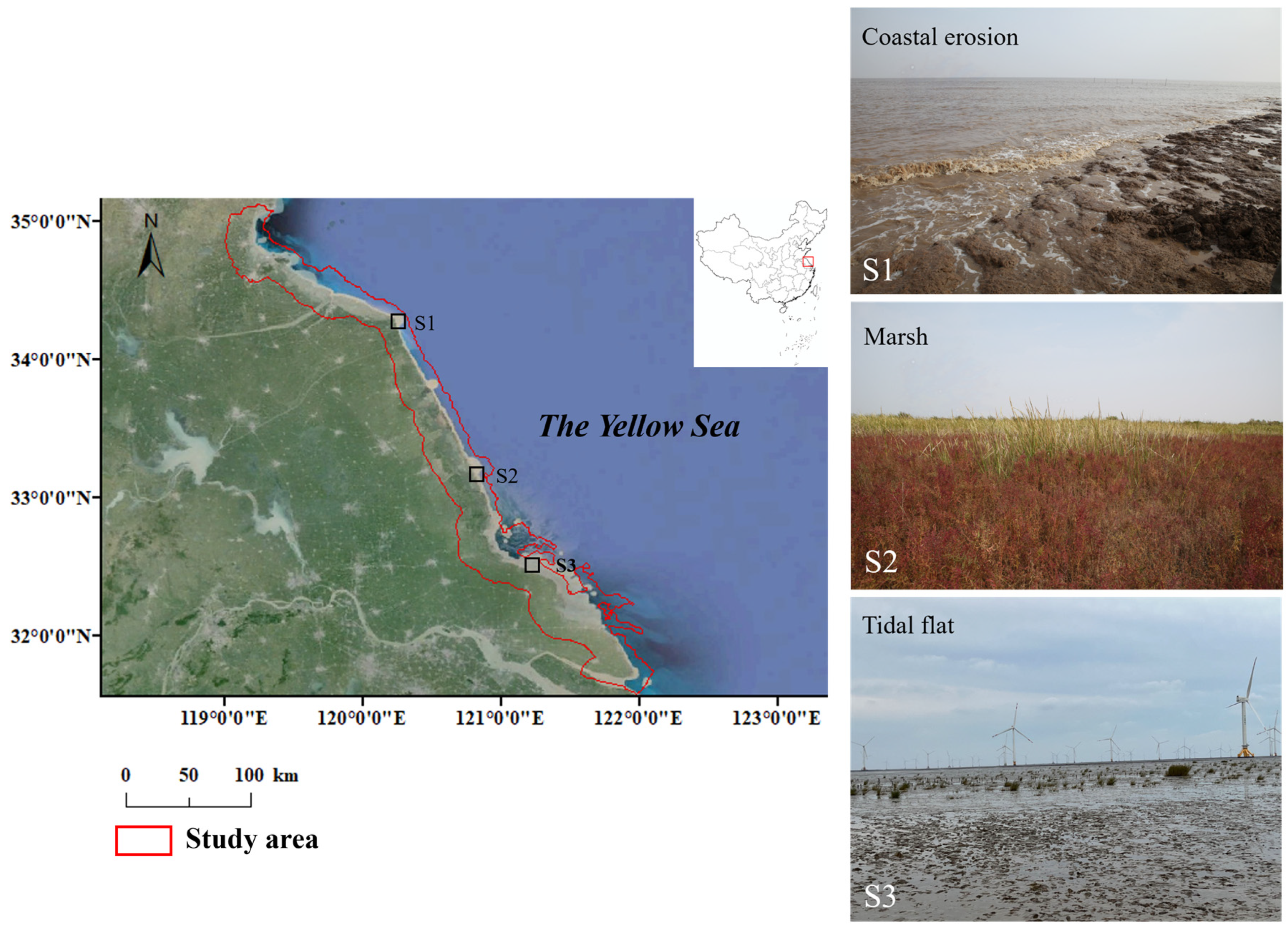
2.1. Study Area

The study area is situated in Jiangsu Province, the east coast of China, facing the Yellow Sea to the east and located between 116°18′~121°57′E and 30°45′~35°20′N (Figure 1). The coastal zone is relatively flat and encompasses various features such as mudflats, sandbanks, estuaries, and bays, among others. The region is rich in ecological resources and hosts diverse ecosystems, including rare wetland plants and animals. The mudflat wetland in the Yellow Sea is located in Nantong, Yancheng, and Lianyungang. Among them, Yancheng is particularly noteworthy due to its two national nature reserves: the Jiangsu Yancheng Wetland National Nature Reserve, famous for its rare bird species, and the Jiangsu Dafeng Elk National Nature Reserve. Both reserves are critical sanctuaries for wildlife and play a significant role in the conservation of the mudflat wetland in China. Additionally, Tiaozini Wetland, located in the Yellow Sea Ecological Zone, covers an area of 3 × 10⁶ ha and is one of the most vital mudflat wetland ecosystems globally. This area also serves as an essential stopover for migratory birds along the East Asia–Australasia flyway. The region experiences a subtropical monsoon climate, with an average annual temperature ranging from 13.6 to 16.1 °C and annual precipitation of 1059 mm, nearly half of which occurs during the summer months.

2.2. Data Source and Data Pre-Processing

Landsat TM/ETM/OLI images (cloud cover of ≤5%) were utilized for the years 1983, 1990, 2000, 2010, and 2020. These images were downloaded from the USGS (https://earthexplorer.usgs.gov/, accessed on 25 March 2023) with a spatial resolution of 30 m. The selected images corresponded to the row numbers 118/38, 119/37, and 120/36. To ensure the accuracy of the results, images were primarily chosen from the months of May to November when the features of the mudflat wetland are more visible due to the lush growth of plants during the rainy season. In cases where specific zones had poor image quality or excessive cloud cover, high-quality images from adjacent months or years were selected as substitutes. For each of the years, images were extracted and classified to facilitate the analysis and characterization of the mudflat wetland.
The Ramsar Convention defines wetlands to include marsh, fen, peatland, and water. In addition, the convention also includes whether the wetland is natural or artificial, permanent or temporary, and whether water is static or flowing, fresh, brackish, or salty, including areas of marine water where the depth at low tide does not exceed 6 m [40]. Currently, this definition of wetlands has been widely accepted in related research around the world. With reference to the Ramsar definition of wetlands, the classification system was determined based on the comprehensive consideration of the terrestrial coverage in the coastal zone of Jiangsu, as well as the purpose and subsequent application of this study. In the classification system, wetland is divided into 3 major categories and 7 subcategories (Table 1). Additionally, we classified paddy fields as vegetation.
We used ENVI 5.6 for pre-processing the Landsat images, including radiation calibration, to enhance the accuracy of the data. The training and validation data were derived from various sources, including high-resolution imagery from Google Earth, UAV multispectral images collected during the field investigation in 2022, published research, and other available data. Although there is a time lag between the acquisition of the validation data and the Landsat OLI images, the impact on the results is negligible due to the minimal occurrence of drastic land use changes between the two years.
Furthermore, the determination of the bilateral boundary in the study area was identified as a crucial step. We referenced another study [41] to establish the boundaries of the mudflat wetland. The first contour at the 6-m ocean depth, obtained from the Shuttle Radar Topography Mission (SRTM) acquired from NASA (https://www.nasa.gov/, accessed on 25 March 2023), was utilized as the seaward boundary of the mudflat wetland. Additionally, the 15 km buffer zone from the coastline to the land was established as the boundary between the inland and mudflat wetland.

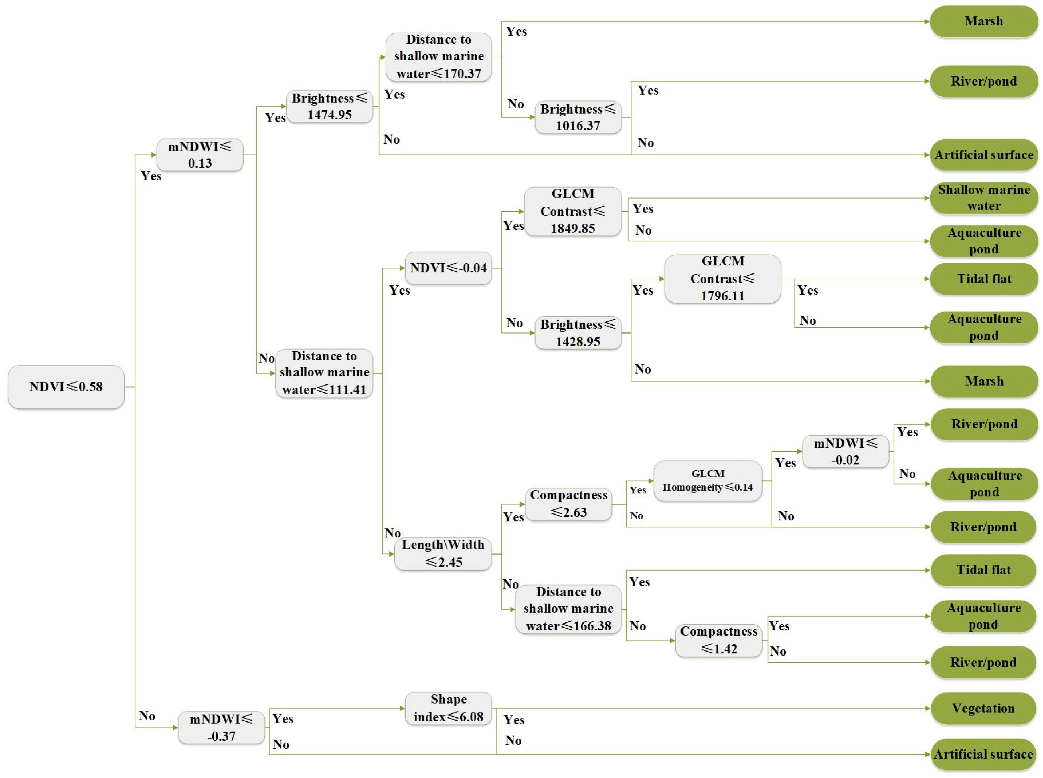
2.3. Extraction Method of Mudflat Wetland

eCognition version 9.2 adopts an image interpretation method that integrates object-oriented and decision tree classification [41]. This method takes into account the feature information of images, including spectral features, geometric features, geographic features, and other factors, which can effectively delineate the object boundaries and identify different object categories within a small area. At the same time, the approach has its advantages in reducing “salt and pepper” effects [32]. After that, we carried out the next step for the processed images. Firstly, multi-resolution segmentation was performed on the pre-processed images. The most important step in this process was the setting of the segmentation scale and other parameters, because small-scale segmentation would generate redundant information, while large-scale segmentation would result in inaccurate wetland boundaries. After checking and comparing the segmentation results of different segmentation scales and consulting the literature, the segmentation scale was finally determined to be 100, the shape index was 0.2, and the tightness index was 0.5. After segmentation was completed, the adjacent similar objects were merged by auxiliary spectral difference segmentation. Secondly, it was necessary to calculate a suitable feature index to construct the decision tree model. For example, the NDVI can effectively separate vegetation from soil and water; the NDWI and mNDWI are effective indicators to identify water bodies. The combination of Brightness and the mNDWI can separate water bodies from tidal flats and marsh; Brightness, the NDVI, and texture characteristics can effectively identify marsh. Geometric features such as length-to-width ratio can distinguish rivers/ponds from aquaculture ponds. The features and calculation formulas used are presented in Table 2.
To classify the images from 2020, a combination of high-resolution imagery from Google Earth and literature data was utilized [41,42,43,44]. The segmented images were classified based on ground objects, and appropriate feature parameters were selected for establishing a decision tree (Figure 2).

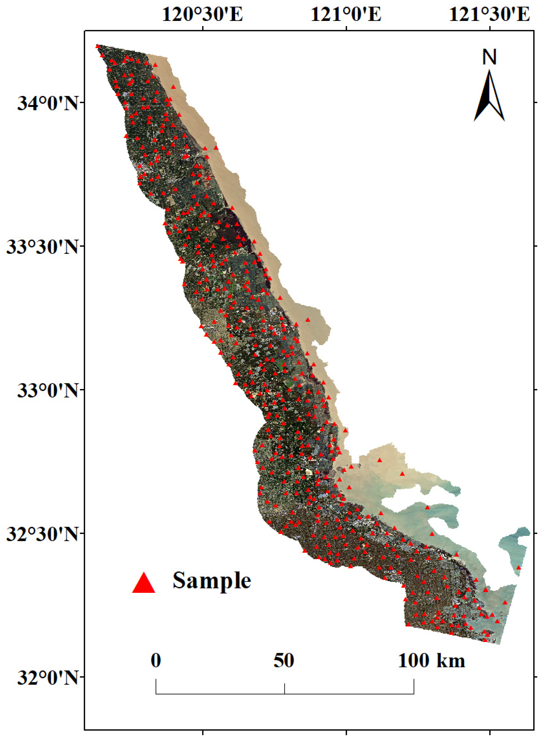
2.4. Classification Accuracy of Mudflat Wetland

In order to verify the accuracy of the classification results, verification samples were established using high-resolution imagery from Google Earth and UAV multispectral images collected during the field investigation in September 2022. To ensure that each category had enough points for validation, we conducted random sampling in the region illustrated in Figure 3 (Path 119/Row 37). A total of 453 points were selected for this purpose. These verification points were used to assess and validate the classification results for the year 2020. After adjusting the decision tree model, we employed the most suitable version to classify the images of the remaining four years. Additionally, any obvious errors in the classification results were corrected through visual inspection.
We employed the confusion matrix to assess the accuracy of the classification, and a total of 453 verification samples were used. As presented in Table 3, the overall accuracy was higher than 90%, and the Kappa coefficient was 0.89. Specifically, shallow marine water exhibits the highest classification accuracy, followed by rivers/ponds. Conversely, the classification accuracy of tidal flats is the lowest, primarily because it is usually intermingled with marsh and shallow marine water, resulting in a characteristic index that was not sufficiently distinct.

2.5. The Construction of the Method of Intertidal Zone Extraction

As a critical area of land–sea interaction, the intertidal zone plays a vital role in understanding coastal dynamics and promoting sustainable coastal development. It is generally submerged at high tide and exposed at low tide. It is the area between the mean low-tide line and the mean high-tide line of the coast [45]. The greatest challenge of intertidal mapping is the invisibility of the intertidal zone. To address this, we considered the combined characteristics of the NDVI, the NDWI, the mNDWI, and other ratio indices. We integrated the blue and green bands to create a high-reflectivity band combination, while employing the short-wave infrared band as a low-reflectivity combination, thereby enhancing the differentiation between sediment water and mudflats. Then, we constructed the IWI (Improved Spectral Water Index) by using ratio and quadratic power operations and calculated it using the following formula:
I W I = ρ B 2 + ρ B 3 ρ B 6 ρ B 7 ρ B 2 + ρ B 3 + ρ B 6 + ρ B 7
where ρ denotes the reflectivity, while B2, B3, B6, and B7 denote OLI blue, green, short-wave infrared I, and short-wave infrared II bands.
The IWI determined by Equation (1) is expected to effectively distinguish between the suspended sediment, coastal vegetation, and tide by making the tide “disappear” during high tide and “appear” during low tide [46]. This would help improve the separability of these features. Given that the intertidal zone in the study area predominantly consists of the muddy flat, it is anticipated that the results would be favorable.
By calculating the coefficient of variation (CV) of the IWI, the dynamic changes in each image set were determined. Subsequently, a threshold value of 0.4 for the CV was applied to extract the intertidal zone. This allowed for the identification of regions with a threshold value greater than 0.4 from the CV images. In order to ensure accurate analysis, it is important to inspect the inland areas as well, as these regions may experience significant changes due to human activities. Therefore, it was necessary to exclude regions with a CV greater than 0.4 in these inland zones. In this way, the analysis becomes more specific to the intertidal zone, thereby improving the accuracy and reliability of the results.

3. Results

3.1. Changes in the Mudflat Wetland

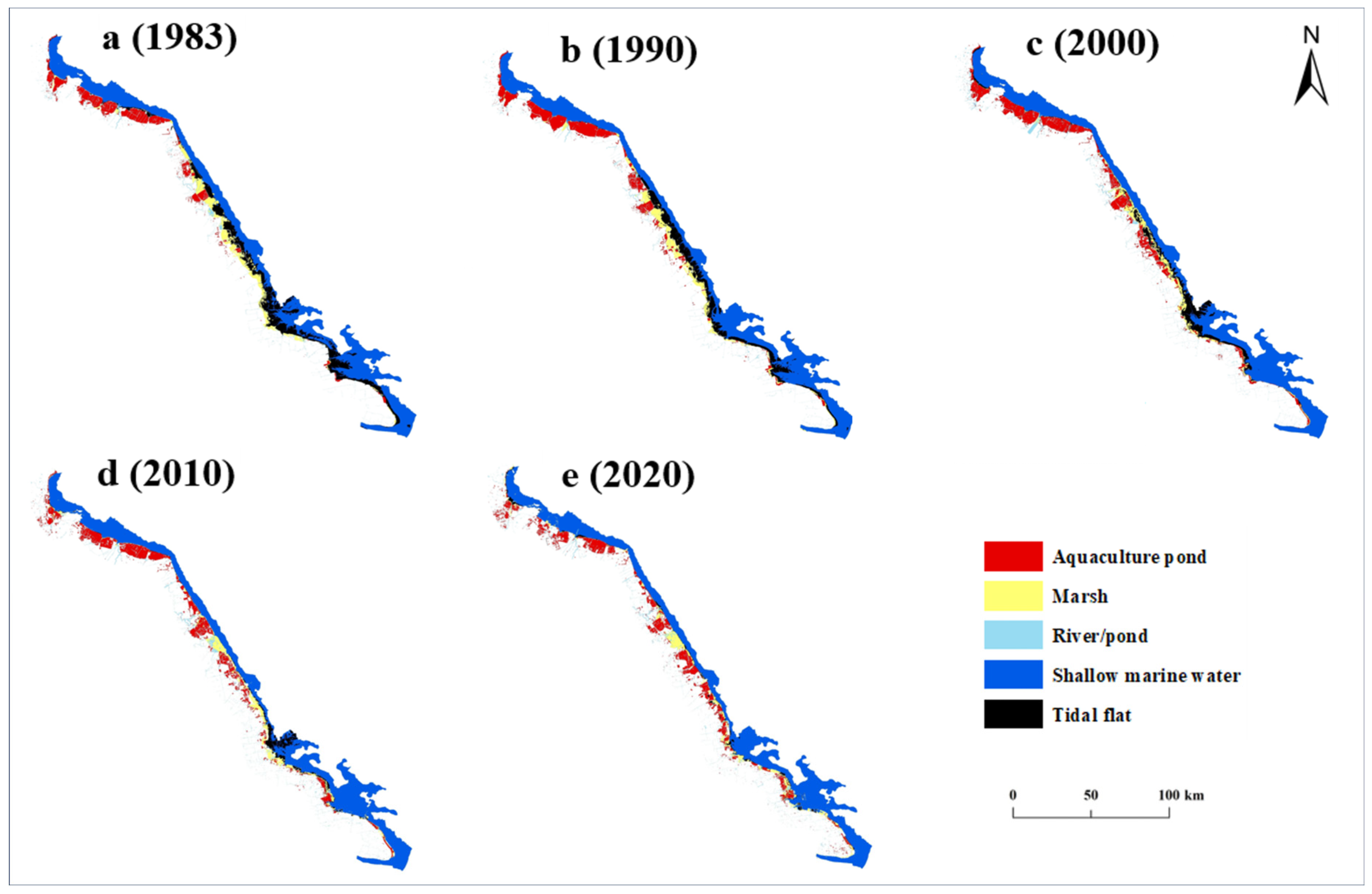
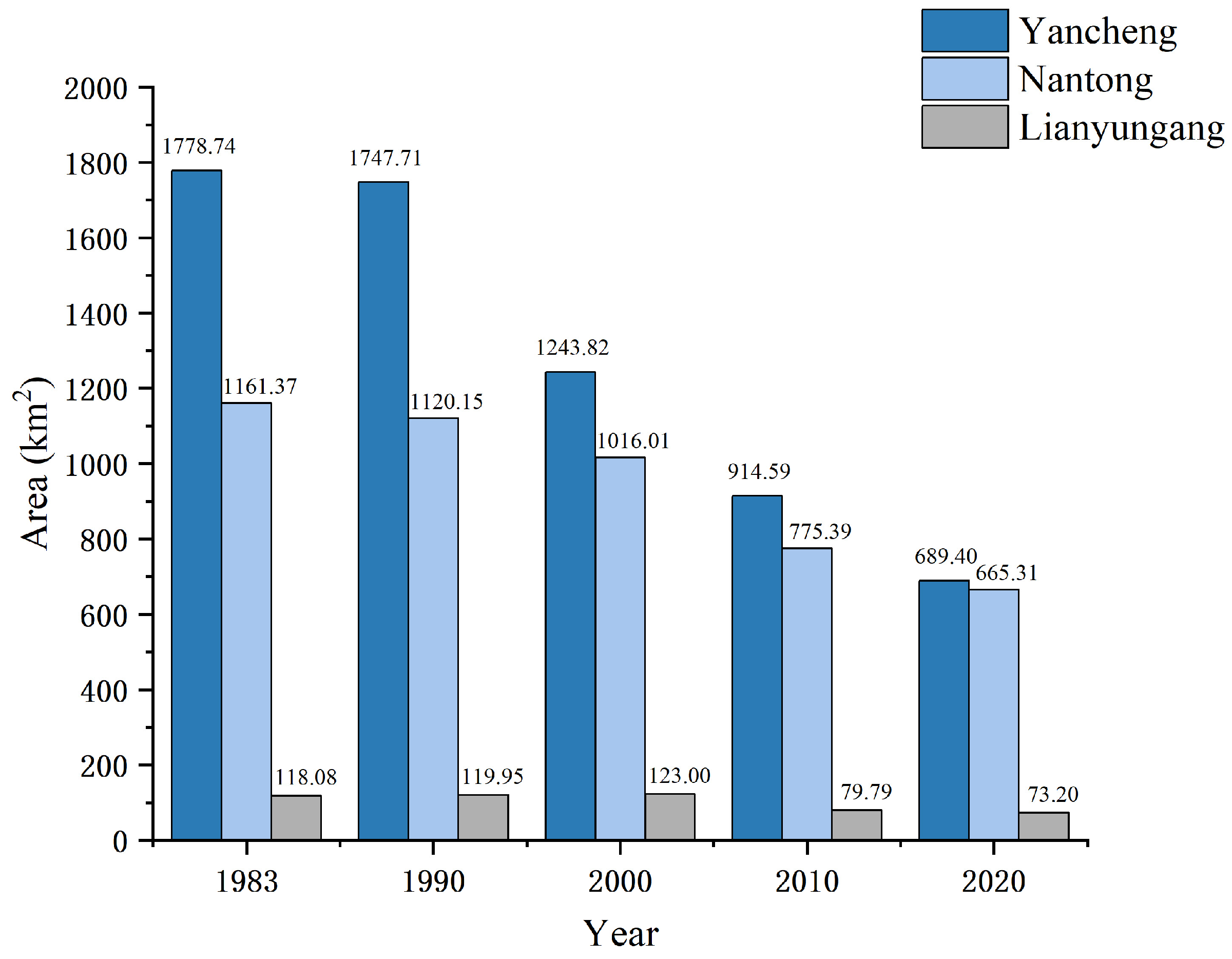
3.1.1. Spatial Changes

The mudflat wetland in the Yellow Sea is distributed along the entire shoreline, as illustrated in Figure 4. It is evident that aquaculture pond area was predominantly located in the central and northern regions of Yancheng and Lianyungang. During this period, the area of aquaculture pond decreased by 137.76 km2 in the northern region, while it increased by 384.26 km2 in the central region and 196.65 km2 in the southern region. Marsh area was primarily concentrated in the central region, with little distribution in the south and north; however, there had been a notable increase of 124.74 km² in the southern region. In the central region, the area of marsh peaked at 612.21 km2 and declined to only 291.28 km² by 2020. Despite an overall decrease in marsh area, the establishment of two national nature reserves in Yancheng has facilitated its recovery, resulting in a slowed rate of area shrinkage after 2010. Among all types of the mudflat wetland, the tidal flat area experienced the most significant loss. Prior to 2010, the tidal flat area was extensively distributed in the central and southern regions, with a peak area of 1772.88 km2. By 2020, however, the area of tidal flat in these two regions dramatically decreased, totaling a reduction of 1600.88 km2. In contrast, the tidal flat area in the northern region underwent minimal change. Additionally, the river/pond area increased by 127.75 km2 in the coastal zone, while shallow marine water expanded by 192.24 km2 in the south but decreased by 226.93 km2 in the central and northern regions.
Overall, the area of the mudflat wetland in the central region experienced the most significant shrinkage, totaling 829.80 km2. However, the rate of this shrinkage was mitigated due to the implementation of conservation policies and regulations. In the northern and southern regions, the mudflat wetland areas decreased by 211.06 km2 and 208.99 km2, respectively. The reduction in the northern region was primarily attributed to the decrease in aquaculture pond area, while in the southern region, the loss was mainly due to the decline in tidal flat area.

3.1.2. Temporal Changes

The area of various land use types in the coastal zone from 1983 to 2020 is illustrated in Figure 5. In 1983, the natural wetland accounted for 49.36% of the entire coastal zone, while the human-made wetland represented 6.47%. By 2020, however, the proportion of the natural wetland decreased to 38.75%, whereas the proportion of the human-made wetland increased to 9.07%.
The results indicate that the tidal flat area experienced the most significant decrease, with an area decrease of 1597.37 km2. In 1983, the tidal flat area was the largest and most important natural wetland, covering an area of 1818.60 km2, which accounted for 11.36% of the study area and 23.01% of the natural wetland. However, by 2020, its area had diminished to only 211.23 km2, equivalent to 1.38% of the study area and 3.56% of the natural wetland. During this same period, marsh area also lost 184.81 km2. In contrast, aquaculture pond area expanded by 416.32 km2. The area of river/pond remained relatively stable, with a notable increase of 131.52 km² observed in 2000. Similarly, shallow marine water maintained an area of 5050 ± 100 km2 throughout this period.
Figure 6 illustrates the changes in the area of the natural and human-made wetlands. The area of the natural wetland continued to decline from 7904.27 km2 to 6205.90 km2 over the period, with a reduction rate of 446.9 km2/10a. The most significant loss occurred between 2000 and 2010, with a total decrease of 647.48 km2. In contrast, the human-made wetland area initially increased rapidly but later declined slowly. It increased by 620.59 km2 from 1983 to 2000, but subsequently shrank by 204.28 km2 over the next two decades.

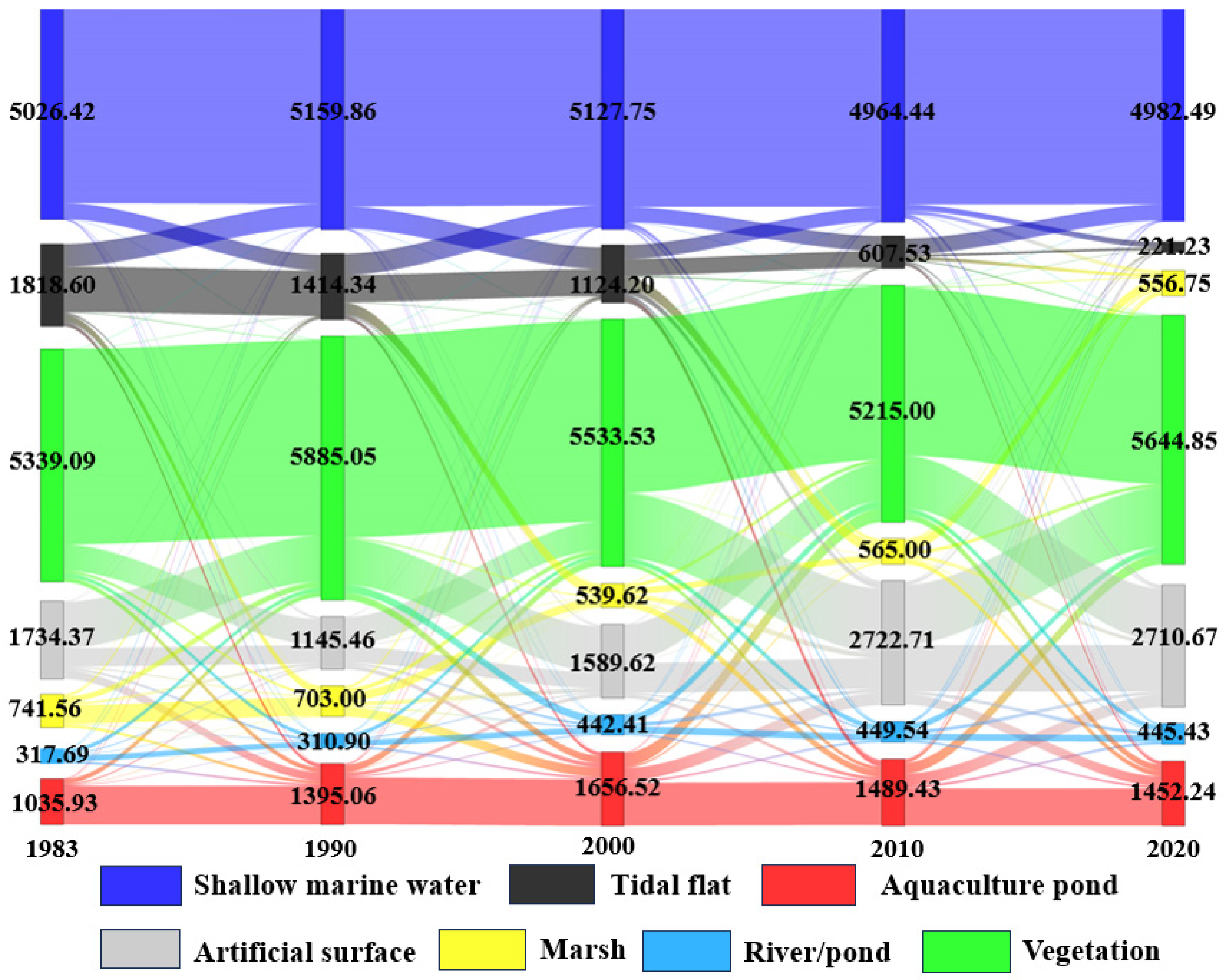
3.2. Land Use Change Trajectories from 1983 to 2020

By using Origin, we obtained the change trajectory of the coastal zone from 1983 to 2020 (Figure 7). The main conversion of the tidal flat area was to aquaculture pond, shallow marine water, and marsh, with areas of 523.58 km2, 438.38 km2, and 311.76 km2, respectively. The first two factors were primarily driven by the development of aquaculture and the processes of coastal erosion and accretion. The third factor was linked to the introduction and rapid expansion of Spartina alterniflora, which encroached upon the tidal flat, displaced other marsh plants, and contributed to consolidate the shoreline. Compared to the results of 2020, marsh areas of 149.84 km2, 115.76 km2, and 361.08 km2 in 1983 were converted to aquaculture pond, artificial surfaces, and vegetation in 2020, respectively. Over these four periods, tidal flat areas of 178.27 km2, 275.40 km2, 281.23 km2, and 81.10 km2 were encroached by marsh due to Spartina alterniflora, which also served as the main conversion pathway into marsh.
During this period, the area of shallow marine water remained relatively stable at about 5000 km2. The primary conversion and encroachment class was tidal flat area, which was closely linked to the dynamic changes in the intensity of coastal erosion and accretion. Vegetation and artificial surfaces were inter-related as major inflows and outflows. Comparing the results of 1983 with 2020, 1441.08 km2 of vegetation was converted to artificial surfaces, while 970.41 km2 of artificial surfaces was converted to vegetation. The area of vegetation exhibited a trend of increasing, followed by a decrease, and then another increase. This fluctuation can largely be attributed to policy changes—from a focus on rapid economic development to an emphasis on high-quality economic development. Additionally, the government established “the red line for the protection of cultivated land”, which was meant to ensure that the area of farmland remains above the minimum. The main conversion of river/pond area and aquaculture pond area was to artificial surfaces and vegetation, with conversion areas of 755.44 km2 and 1584.16 km2. The primary encroachment classes of aquaculture pond area were tidal flat and marsh areas, mainly due to the transformation of the natural mudflat wetland for the development of aquaculture.

3.3. Results and Validation of Intertidal Zone Extraction

The extraction results of the intertidal zone during 1983–2020 are presented in Figure 8a–e. The area of the intertidal zone was 3058.18 km2 in 1983, decreasing to 2987.81 km2 in 1990, 2382.83 km2 in 2000, 1769.77 km2 in 2010, and 1427.91 km2 in 2020. Over this period, the intertidal zone decreased by 53.31%, totaling a loss of 1630.27 km2, with a reduction rate of 429.02 km2 per decade. The most dramatic changes occurred between 1990 and 2010, with a decrease of approximately 600 km2 per decade. From 2010 to 2020, the area declined at a slower rate of 341.86 km2. The zoomed-in plots in Figure 8a–e represent the radial sand ridges in the Yellow Sea, which have increased in area over the study period. These radial sand ridges are among the few intertidal regions that have shown significant expansion, effectively slowing the shrinkage of the intertidal zone in the Yellow Sea and preserving local ecological benefits to some extent.
There are differences in the changes in the intertidal zone across various regions (Figure 9). The muddy intertidal zone in the Yellow Sea is primarily concentrated in Yancheng and Nantong, which together comprise over 94.5% of the total area. Over the past 40 years, the intertidal zone in both Yancheng and Nantong has experienced continuous shrinkage. The most significant reduction occurred in Yancheng between 1990 and 2000, where a total loss of 503.89 km² was recorded. The intertidal zone area in Yancheng decreased from 1778.74 km² in 1983 to only 689.40 km² in 2020, reflecting a decrease of 61.24%. Similarly, Nantong lost 496.06 km² of its intertidal zone, resulting in a loss rate of 42.71%. In contrast, the situation in Lianyungang differs slightly from the other two regions. From 1983 to 2000, the intertidal zone area in Lianyungang remained relatively stable at 120 km² approximately. However, between 2000 and 2010, it experienced significant shrinkage, with a reduction rate of 35.13% and a total loss of 43.21 km². Overall, the muddy intertidal zone in the Yellow Sea has undergone substantial area shrinkage from 1990 to 2010; however, the rate of reduction slowed after 2010.
To validate the accuracy of extracting the muddy intertidal zone using the IWI, we compared the results with publicly available global intertidal zone data [47]. Due to the absence of global intertidal zone data for 2020, we chose to compare the results from 2000 and 2010. The results reveal that the extraction results using the IWI closely align with the global intertidal zone data, showing a comparison error of approximately 12% for both datasets (Table 4). Furthermore, the area shrinkage rates from 2000 to 2010 are comparable, both around 25%. These findings suggest that the IWI demonstrates a high level of accuracy in extracting the muddy intertidal zone.

4. Discussion

4.1. Object-Oriented and Decision Tree Classification and the IWI

As the separation of mudflat wetland from other land cover types is usually easier than separation within wetland categories [48], in addition to the comprehensive consideration of various image features, object-oriented and decision tree classification achieved good classification accuracy. Compared to traditional visual interpretation, object-oriented and decision tree classification offers higher classification efficiency and is more suitable for large-scale wetland mapping [28]. Furthermore, this method is able to address “salt and pepper” effects better, thereby enhancing classification accuracy. It is important to note that the appropriate setting of the segmentation scale and other parameters significantly impacts the final results. While the parameters we used are effective for extracting mudflat wetlands, optimal parameters will need to be determined for extracting other types of wetlands.
Many scholars have conducted studies on the extraction of the muddy intertidal zone in China [49,50]. However, these studies often overlooked the dynamic nature of intertidal mapping. Long-term remote sensing datasets can effectively identify the dynamic changes within the intertidal zone. By calculating the CV based on the IWI of each image, we could capture these changes. The variations influenced by tides and human activities in both coastal and inland areas were effectively documented. By establishing thresholds and manually removing errors, we successfully minimized misclassifications in these regions. The IWI emphasizes the distinction of sediment-laden water and muddy flats, resulting in high accuracy for extracting the muddy intertidal zone. However, its effectiveness for other parts of the intertidal zone, such as the sandy intertidal zone, still needs to be validated.

4.2. Impact of Ocean Dynamics

According to the sixth report of the Intergovernmental Panel on Climate Change (IPCC), coastlines are projected to push seaward. There are many studies indicating that the coastline of Jiangsu has been constantly advancing toward the sea [51,52]. Since the 1980s, the average seaward advancing speed of the Jiangsu coastline has been 30.42 m/a, and the speed has been accelerating [52]. Coastal accretion is one of the important reasons. Under the influence of tidal hydrodynamics, the tidal flats have rapidly expanded toward the ocean. The protection of beach vegetation counteracted the impacts of erosion so that the coastline moved seaward. The bedrock coastal crust in the Lianyungang area has also been rising [53]. The newly accreted beach has become an excellent site for the construction of aquaculture ponds, which facilitated the rapid development of the coastal aquaculture industry.
Certain areas have also experienced severe erosion due to seawater, resulting in the loss of tidal flats. The north side of Yueliang Bay–Sheyang Estuary (120°16′~120°29′E, 33°49′~34°15′N), located near Abandoned Yellow River Delta, has witnessed significant erosion, resulting in the washing away of numerous aquaculture ponds along the coast. The phenomenon began in the 1990s, during which some embankments were breached, causing farmland and aquaculture operations to retreat and forcing local residents to relocate. This situation severely impacted the lives and economic activities of the local population. After the dikes were breached, the shoreline retreated and the marine water inundated additional areas, resulting in a reduction in the intertidal zone.

4.3. The Impact of Artificial Consolidation of the Shoreline

Jiangsu coastline was dominated by artificial coastlines from 1985 to 2020 [54] because of human activities such as the construction of dikes. The government hopes to acquire more land in this way. A great deal of reclamation took place during this period. From 1990 to 2000 alone, the area of reclamation reached 399.35 km2 [54]. The expansion of most dikes and dams reflects the trend of coastal siltation [55]. The dike reduces the carrying capacity of the tidal current and exacerbates siltation. The evolution pattern of “upward siltation and downward intrusion” formed around the transition zone is the geomorphic response mode of coastal tidal flat reclamation activities [56]. It should be noted that even the most robust dikes may still be susceptible to destruction. While the construction of coastal dikes is often regarded as the simplest and most direct solution to combat coastal erosion, future research should focus on utilizing biological methods for ecological prevention and control to stabilize shorelines. As an example, oysters were strategically planted along the coast of Staten Island as a natural alternative to concrete dikes in the United States [57]. This innovative approach not only provides protection against storm surges but also contributes to the purification of seawater.
In Jiangsu’s coastal zone, Spartina alterniflora was introduced in the past to stabilize the shoreline in Yancheng coast, and it played its expected role. Unfortunately, it has now become a significant threat to the local ecological environment as an invasive species due to its ability to reproduce quickly, which has led to the continuous encroachment on tidal flats and the habitat of Suaeda salsa, a crucial local species. As a result, extensive efforts have been implemented to control its spread and mitigate its negative impacts.

4.4. Impact of Socio-Economic Development and Policies

We analyzed the correlation between the area of the mudflat wetland, the population, and GDP based on the data obtained from the Jiangsu Statistical Yearbook (JSY) to assess the impact of socio-economic development on the mudflat wetland (Figure 10). The natural wetland, non-wetland, and intertidal zone exhibit a very strong positive correlation with both population and economy. There is a high positive correlation between the human-made wetland and population, along with a moderate positive correlation with GDP. Conversely, the natural wetland shows varying degrees of negative correlation with the human-made wetland and non-wetland, indicating that their expansion has encroached upon significant portions of the natural wetland.
In 1982, the permanent resident population of Jiangsu Province was 60,521,100, while by 2020, the number had increased to 84,748,000, representing a growth rate of 40.03%. This population growth significantly heightened the demand for arable land and housing, leading to accelerated land development activities, including land reclamation, expansion of built-up areas, and increases in agricultural land and industrial sites. Numerous canals, channels, and ditches were constructed to meet the growing needs for irrigation. In order to implement government policies of economic growth, many grass flat and reed areas were reclaimed and transformed into aquaculture ponds to obtain greater economic benefits compared with the modest economic benefits of agriculture [42]. These human activities have caused great disturbance to the natural wetland ecosystem. Land use underwent dramatic changes during this period.
In order to vigorously develop the economy, Jiangsu began to construct many factories and development zones in the coastal zone, starting in the 1980s, which led to significant wetland occupation. According to the JSY, the GDP of Jiangsu Province increased by more than 230 times over the 38 years, while the GDP of the three coastal cities of Nantong, Yancheng, and Lianyungang also grew by more than 190 times. The rapid development of the economy required the occupation of a mass portion of the wetland. The government began to promote a strategy known as “constructing marine eastern Jiangsu” in Donghai of Jiangsu Province in the 1990s. It issued corresponding preferential policies to promote the development of the aquaculture industry, which led to large-scale sea reclamation. The land area of Jiangsu increased by 107,378 ha from 1984 to 2016, with sea reclamation accounting for 98,520 ha [58]. Consequently, vast areas of the natural wetland and intertidal zone were developed into aquaculture ponds and agricultural land. The output of aquatic products in Jiangsu rose dramatically from 6.75 × 10⁵ t in 1985 to 4.90 × 10⁶ t in 2020, peaking at 5.2 × 10⁶ t in 2015. With the development of Jiangsu’s coastal aquaculture industry, significant areas of marsh, shallow marine water, and tidal flats were converted into aquaculture ponds. This alteration in the landscape resulted in ecological degradation, severely diminishing the ecological benefits provided by the mudflat wetland.
Around 2010, the government realized the shortcomings of the previous development model, which prioritized economic growth at the expense of environmental degradation. As a result, there was a shift toward emphasizing environmental protection, exemplified by the promotion of the principle that “Lucid waters and lush mountains are invaluable assets” and the implementation of related policies. In areas with excessive silt, such as Dafeng and Dongtai, the government introduced plants that moisten and remove silt. These initiatives have helped protect the coastline and slowed the rate of coastline siltation [59]. Consequently, between 2010 and 2020, there was a noticeable decrease in the rate of shrinkage of the natural wetland and intertidal zone compared to the previous decade. However, it is worth noting that the policy of returning aquaculture pond to agricultural land, intended to address future food security concerns, has also had an impact on human-made wetland in the coastal zone, resulting in its decline since 2010.
This study suggests that effectively protecting the natural mudflat wetland and reducing human encroachment are urgent and critical issues facing the mudflat wetland in the Yellow Sea. Human intervention is not absolutely negative in the protection of the mudflat wetland in the Yellow Sea. Scientific and reasonable human assistance measures can be more beneficial to the healthy development of ecosystems [36,60]. It is essential to preserve the original natural landscape as much as possible when conducting human interventions, while also reasonably planning for productive land use to maximally meet the needs of economic and social development. There is no doubt that the establishment of nature reserves alone is not enough, but also the complex interplay of ecological and social relationships throughout the coastal ecoregion needs to be considered.

5. Conclusions

(1)
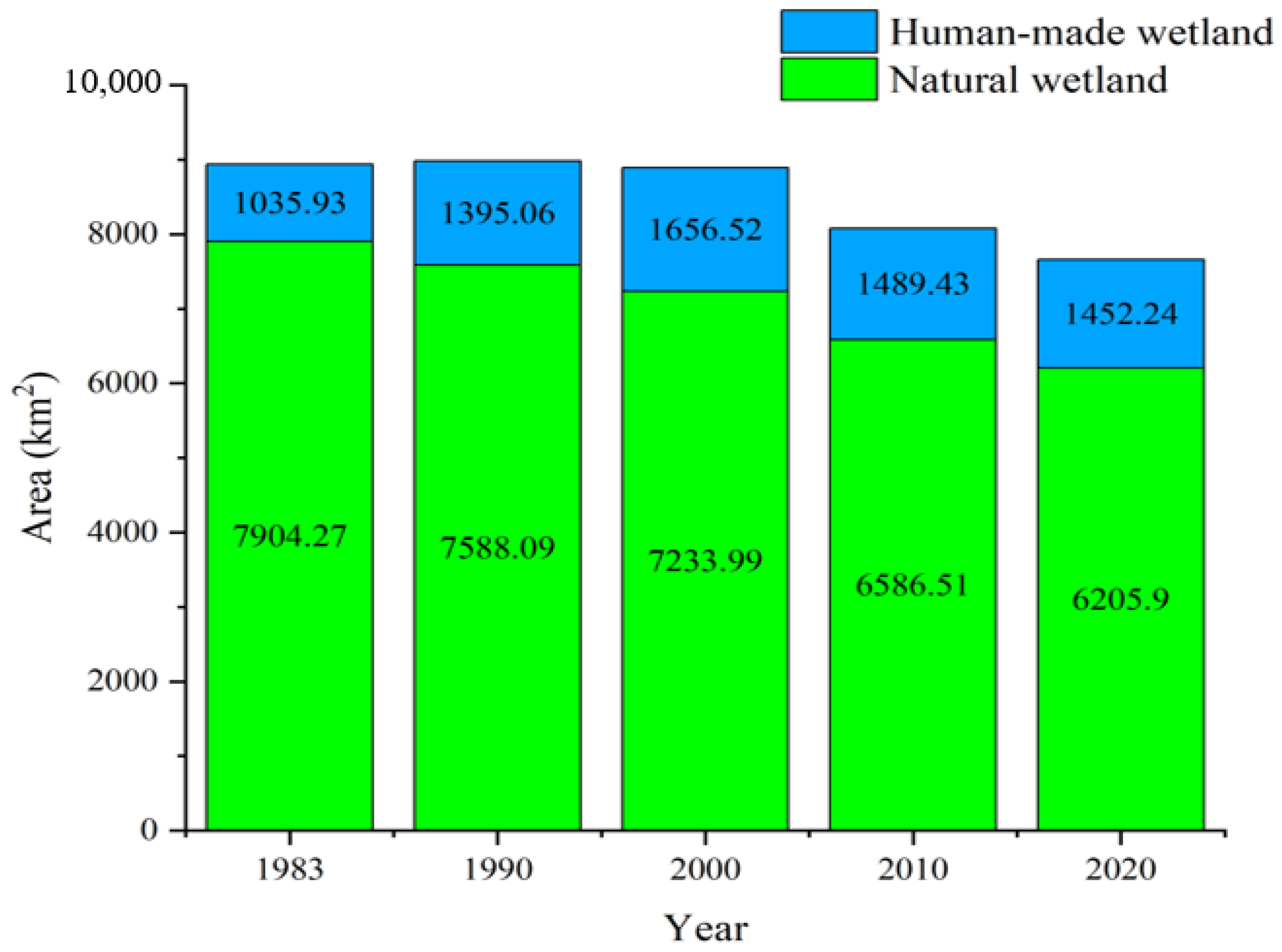
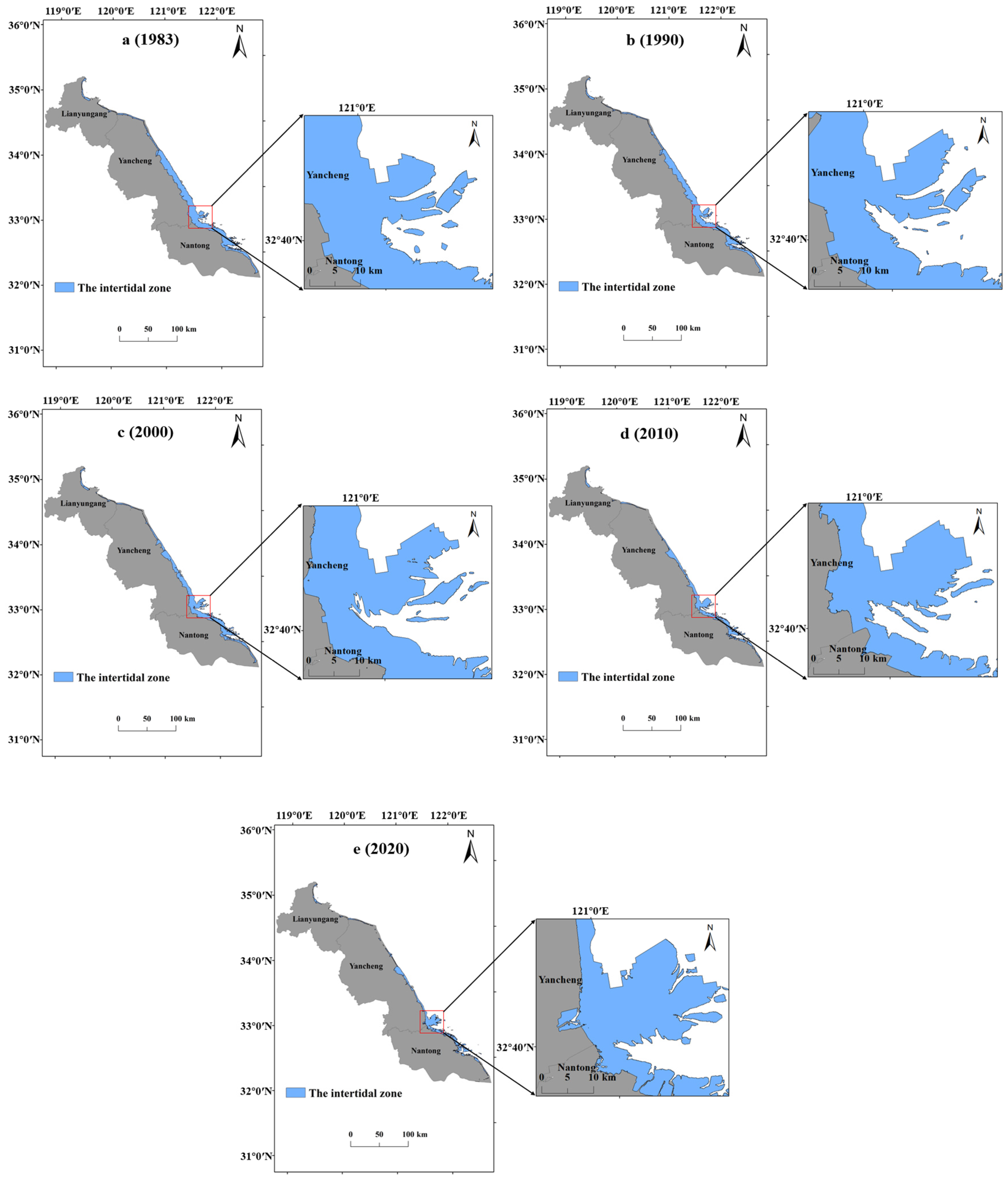
Object-oriented and decision tree classification and the IWI are highly effective methods for extracting the mudflat wetland and muddy intertidal zone. The mudflat wetland area in the Yellow Sea decreased from 8940.20 km2 in 1983 to 7658.14 km2 by 2020, with a reduction rate of 337.38 km2/10a. The area of the natural mudflat wetland decreased by 446.94 km2/10a, while the human-made wetland increased by 109.56 km2/10a. Additionally, the area of the intertidal zone, which covered 3058.18 km2 in 1983, experienced a decline of 429.02 km2/10a.
(2)
Affected by factors like the economy, policy, ocean dynamics, and species invasion, the area of the natural mudflat wetland and intertidal zone in the Yellow Sea had been shrinking at a similar rate. Both of them had a decrease of about 45 km2/a, with significant changes occurring between 2000 and 2010. The main loss type of the natural wetland was tidal flats, followed by marsh. Conversely, the human-made wetland was increasing, driven by factors such as reclamation.
(3)
At present, the policies related to wetland protection have achieved some positive outcomes. It is suggested that wetland protection work should be further deepened from the following aspects: further improving the laws and regulations of wetland protection and the protection system of wetland reserves; establishing extensive wetland ecological monitoring sites to detect changes in the wetland ecosystem over time; and strengthening publicity and education to build public awareness of wetland protection.

Author Contributions

Conceptualization, Z.H. and W.T.; data curation, Z.H. and C.Z.; formal analysis, C.J. and J.Z.; funding acquisition, C.Z. and C.J.; investigation, Z.H., W.T. and C.Z.; methodology, Z.H., W.T. and C.Z.; project administration, C.Z. and C.J.; resources, C.Z. and C.J.; software, Z.H. and W.T.; supervision, C.Z., C.J. and J.Z.; validation, Z.H. and W.T.; visualization, Z.H. and W.T.; writing—original draft, Z.H. and W.T.; writing—review and editing, C.Z. and J.Z. All authors have read and agreed to the published version of the manuscript.

Funding

This research was funded by the key project of the National Natural Science Foundation (42130405).

Data Availability Statement

The Landsat images were downloaded from https://developers.google.cn/earth-engine/ (accessed on 25 March 2023). The SRTM data were downloaded from NASA (https://www.nasa.gov/, accessed on 25 March 2023).

Acknowledgments

The authors give thanks to Tao Zhang for his help with the UAV during the field investigation in 2022. We would also like to express our sincere gratitude to the editor and anonymous reviewers for their insightful and constructive comments.

Conflicts of Interest

The authors declare no conflicts of interest.

References

  1. Boak, E.H.; Turner, I.L. Shoreline definition and detection: A review. J. Coast. Res. 2005, 21, 688–703. [Google Scholar] [CrossRef]
  2. Mujabar, P.S.; Chandrasekar, N. Shoreline change analysis along the coast between Kanyakumari and Tuticorin of India using remote sensing and GIS. Arab. J. Geosci. 2013, 6, 647–664. [Google Scholar] [CrossRef]
  3. Wang, Z.; Wu, J.; Madden, M.; Mao, D. China’s wetlands: Conservation plans and policy impacts. Ambio 2012, 41, 782–786. [Google Scholar] [CrossRef] [PubMed]
  4. Ramachandran, A.; Enserink, B.; Balchand, A. Coastal regulation zone rules in coastal panchayats (villages) of Kerala, India vis-à-vis socio-economic impacts from the recently introduced peoples’ participatory program for local self-governance and sustainable development. Ocean Coast. Manag. 2005, 48, 632–653. [Google Scholar] [CrossRef]
  5. Houghton, J.T.; Ding, Y.; Griggs, D.J.; Noguer, M.; van der Linden, P.J.; Dai, X.; Maskell, K.; Johnson, C.A. Climate Change 2001: The Scientific Basis; Cambridge University Press: Cambridge, UK, 2001; Volume 881. [Google Scholar]
  6. Asselen, S.v.; Verburg, P.H.; Vermaat, J.E.; Janse, J.H. Drivers of wetland conversion: A global meta-analysis. PLoS ONE 2013, 8, e81292. [Google Scholar] [CrossRef]
  7. Kirwan, M.L.; Megonigal, J.P. Tidal wetland stability in the face of human impacts and sea-level rise. Nature 2013, 504, 53–60. [Google Scholar] [CrossRef]
  8. Mao, D.; Wang, Z.; Wu, J.; Wu, B.; Zeng, Y.; Song, K.; Yi, K.; Luo, L. China’s wetlands loss to urban expansion. Land Degrad. Dev. 2018, 29, 2644–2657. [Google Scholar] [CrossRef]
  9. Niu, Z.; Gong, P.; Cheng, X.; Guo, J.; Wang, L.; Huang, H.; Shen, S.; Wu, Y.; Wang, X.; Wang, X. Geographical characteristics of China’s wetlands derived from remotely sensed data. Sci. China Ser. D Earth Sci. 2009, 52, 723–738. [Google Scholar] [CrossRef]
  10. National Forestry and Grassland Administration. The Report on the Second National Wetland Resources Survey (2009–2013). 2014. Available online: https://www.forestry.gov.cn/main/65/20140128/758154.html (accessed on 25 March 2023). (In Chinese)
  11. Nahlik, A.M.; Fennessy, M.S. Carbon storage in US wetlands. Nat. Commun. 2016, 7, 13835. [Google Scholar] [CrossRef]
  12. Zhu, P.; Gong, P. Suitability mapping of global wetland areas and validation with remotely sensed data. Sci. China Earth Sci. 2014, 57, 2283–2292. [Google Scholar] [CrossRef]
  13. Wang, W.; Sardans, J.; Wang, C.; Zeng, C.; Tong, C.; Chen, G.; Huang, J.; Pan, H.; Peguero, G.; Vallicrosa, H. The response of stocks of C, N, and P to plant invasion in the coastal wetlands of China. Glob. Change Biol. 2019, 25, 733–743. [Google Scholar] [CrossRef] [PubMed]
  14. Xia, S.; Song, Z.; Van Zwieten, L.; Guo, L.; Yu, C.; Wang, W.; Li, Q.; Hartley, I.P.; Yang, Y.; Liu, H. Storage, patterns and influencing factors for soil organic carbon in coastal wetlands of China. Glob. Change Biol. 2022, 28, 6065–6085. [Google Scholar] [CrossRef]
  15. Cui, B.; He, Q.; Gu, B.; Bai, J.; Liu, X. China’s coastal wetlands: Understanding environmental changes and human impacts for management and conservation. Wetlands 2016, 36, 1–9. [Google Scholar] [CrossRef]
  16. Murray, N.J.; Clemens, R.S.; Phinn, S.R.; Possingham, H.P.; Fuller, R.A. Tracking the rapid loss of tidal wetlands in the Yellow Sea. Front. Ecol. Environ. 2014, 12, 267–272. [Google Scholar] [CrossRef]
  17. Chen, S.-s.; Chen, L.-f.; Liu, Q.-h.; Li, X.; Tan, Q. Remote sensing and GIS-based integrated analysis of coastal changes and their environmental impacts in Lingding Bay, Pearl River Estuary, South China. Ocean Coast. Manag. 2005, 48, 65–83. [Google Scholar] [CrossRef]
  18. Sarma, P.K.; Lahkar, B.P.; Ghosh, S.; Rabha, A.; Das, J.P.; Nath, N.K.; Dey, S.; Brahma, N. Land-use and land-cover change and future implication analysis in Manas National Park, India using multi-temporal satellite data. Curr. Sci. 2008, 95, 223–227. [Google Scholar]
  19. Green, E.P.; Clark, C.; Mumby, P.; Edwards, A.; Ellis, A. Remote sensing techniques for mangrove mapping. Int. J. Remote Sens. 1998, 19, 935–956. [Google Scholar] [CrossRef]
  20. Seto, K.C.; Fragkias, M. Quantifying spatiotemporal patterns of urban land-use change in four cities of China with time series landscape metrics. Landsc. Ecol. 2005, 20, 871–888. [Google Scholar] [CrossRef]
  21. Kumar, P.D.; Gopinath, G.; Laluraj, C.; Seralathan, P.; Mitra, D. Change detection studies of Sagar Island, India, using Indian remote sensing satellite 1C linear imaging self-scan sensor III data. J. Coast. Res. 2007, 23, 1498–1502. [Google Scholar] [CrossRef]
  22. Barducci, A.; Guzzi, D.; Marcoionni, P.; Pippi, I. Aerospace wetland monitoring by hyperspectral imaging sensors: A case study in the coastal zone of San Rossore Natural Park. J. Environ. Manag. 2009, 90, 2278–2286. [Google Scholar] [CrossRef] [PubMed]
  23. Amani, M.; Brisco, B.; Afshar, M.; Mirmazloumi, S.M.; Mahdavi, S.; Mirzadeh, S.M.J.; Huang, W.; Granger, J. A generalized supervised classification scheme to produce provincial wetland inventory maps: An application of Google Earth Engine for big geo data processing. Big Earth Data 2019, 3, 378–394. [Google Scholar] [CrossRef]
  24. Mahdavi, S.; Salehi, B.; Granger, J.; Amani, M.; Brisco, B.; Huang, W. Remote sensing for wetland classification: A comprehensive review. GISci. Remote Sens. 2018, 55, 623–658. [Google Scholar] [CrossRef]
  25. Rezaee, M.; Mahdianpari, M.; Zhang, Y.; Salehi, B. Deep convolutional neural network for complex wetland classification using optical remote sensing imagery. IEEE J. Sel. Top. Appl. Earth Obs. Remote Sens. 2018, 11, 3030–3039. [Google Scholar] [CrossRef]
  26. Gallant, A.L. The challenges of remote monitoring of wetlands. Remote Sens. 2015, 7, 10938–10950. [Google Scholar] [CrossRef]
  27. Mui, A.; He, Y.; Weng, Q. An object-based approach to delineate wetlands across landscapes of varied disturbance with high spatial resolution satellite imagery. ISPRS J. Photogramm. Remote Sens. 2015, 109, 30–46. [Google Scholar] [CrossRef]
  28. Zhang, L.; Li, X.; Yuan, Q.; Liu, Y. Object-based approach to national land cover mapping using HJ satellite imagery. J. Appl. Remote Sens. 2014, 8, 083686. [Google Scholar] [CrossRef]
  29. Blaschke, T. Object based image analysis for remote sensing. ISPRS J. Photogramm. Remote Sens. 2010, 65, 2–16. [Google Scholar] [CrossRef]
  30. Dronova, I. Object-based image analysis in wetland research: A review. Remote Sens. 2015, 7, 6380–6413. [Google Scholar] [CrossRef]
  31. Campbell, A.; Wang, Y. Examining the influence of tidal stage on salt marsh mapping using high-spatial-resolution satellite remote sensing and topobathymetric LiDAR. IEEE Trans. Geosci. Remote Sens. 2018, 56, 5169–5176. [Google Scholar] [CrossRef]
  32. Dronova, I.; Gong, P.; Wang, L. Object-based analysis and change detection of major wetland cover types and their classification uncertainty during the low water period at Poyang Lake, China. Remote Sens. Environ. 2011, 115, 3220–3236. [Google Scholar] [CrossRef]
  33. Zhu, H.; Qin, P.; Wang, H. Functional group classification and target species selection for Yancheng Nature Reserve, China. Biodivers. Conserv. 2004, 13, 1335–1353. [Google Scholar] [CrossRef]
  34. Zhang, H.; Zhen, Y.; Li, Y.; Sun, X. Spatial heterogeneity of soil salinity in Jiangsu Yancheng Wetland National Nature Reserve rare birds. Wetl. Sci 2018, 16, 152–158. [Google Scholar]
  35. Ou, W.; Yang, G.; Li, H.-P.; Yu, X. Spatio-temporal variation and driving forces of landscape patterns in the coastal zone of Yancheng, Jiangsu. Sci. Geogr. Sin. 2004, 24, 610–615. [Google Scholar]
  36. Zuo, P.; Wan, S.W.; Qin, P.; Du, J.; Wang, H. A comparison of the sustainability of original and constructed wetlands in Yancheng Biosphere Reserve, China: Implications from emergy evaluation. Environ. Sci. Policy 2004, 7, 329–343. [Google Scholar] [CrossRef]
  37. Sun, Z.; Sun, W.; Tong, C.; Zeng, C.; Yu, X.; Mou, X. China’s coastal wetlands: Conservation history, implementation efforts, existing issues and strategies for future improvement. Environ. Int. 2015, 79, 25–41. [Google Scholar] [CrossRef]
  38. Niu, Z.; Zhang, H.; Gong, P. More protection for China’s wetlands. Nature 2011, 471, 305. [Google Scholar] [CrossRef]
  39. An, S.; Li, H.; Guan, B.; Zhou, C.; Wang, Z.; Deng, Z.; Zhi, Y.; Liu, Y.; Xu, C.; Fang, S. China’s natural wetlands: Past problems, current status, and future challenges. AMBI A J. Hum. Environ. 2007, 36, 335–342. [Google Scholar] [CrossRef]
  40. Gong, P.; Niu, Z.; Cheng, X.; Zhao, K.; Zhou, D.; Guo, J.; Liang, L.; Wang, X.; Li, D.; Huang, H. China’s wetland change (1990–2000) determined by remote sensing. Sci. China Earth Sci. 2010, 53, 1036–1042. [Google Scholar] [CrossRef]
  41. Mao, D.; Wang, Z.; Du, B.; Li, L.; Tian, Y.; Jia, M.; Zeng, Y.; Song, K.; Jiang, M.; Wang, Y. National wetland mapping in China: A new product resulting from object-based and hierarchical classification of Landsat 8 OLI images. ISPRS J. Photogramm. Remote Sens. 2020, 164, 11–25. [Google Scholar] [CrossRef]
  42. Ke, C.-Q.; Zhang, D.; Wang, F.-Q.; Chen, S.-X.; Schmullius, C.; Boerner, W.-M.; Wang, H. Analyzing coastal wetland change in the Yancheng national nature reserve, China. Reg. Environ. Change 2011, 11, 161–173. [Google Scholar] [CrossRef]
  43. Zang, Z.; Zou, X.; Zuo, P.; Song, Q.; Wang, C.; Wang, J. Impact of landscape patterns on ecological vulnerability and ecosystem service values: An empirical analysis of Yancheng Nature Reserve in China. Ecol. Indic. 2017, 72, 142–152. [Google Scholar] [CrossRef]
  44. Xu, C.; Pu, L.; Zhu, M.; Li, J.; Chen, X.; Wang, X.; Xie, X. Ecological security and ecosystem services in response to land use change in the coastal area of Jiangsu, China. Sustainability 2016, 8, 816. [Google Scholar] [CrossRef]
  45. Shen, F.; Gao, A.; Wu, J.; Zhou, Y.; Zhang, J. A remotely sensed approach on waterline extraction of silty tidal flat for DEM construction, a case study in Jiuduansha Shoal of Yangtze River. Acta Geod. Cartogr. Sin. 2008, 37, 102–107. [Google Scholar]
  46. Tang, W.; Zhao, C.; Lin, J.; Jiao, C.; Zheng, G.; Zhu, J.; Pan, X.; Han, X. Improved spectral water index combined with Otsu algorithm to extract muddy coastline data. Water 2022, 14, 855. [Google Scholar] [CrossRef]
  47. Murray, N.J.; Phinn, S.R.; DeWitt, M.; Ferrari, R.; Johnston, R.; Lyons, M.B.; Clinton, N.; Thau, D.; Fuller, R.A. The global distribution and trajectory of tidal flats. Nature 2019, 565, 222–225. [Google Scholar] [CrossRef]
  48. Ozesmi, S.L.; Bauer, M.E. Satellite remote sensing of wetlands. Wetl. Ecol. Manag. 2002, 10, 381–402. [Google Scholar] [CrossRef]
  49. Murray, N.J.; Phinn, S.R.; Clemens, R.S.; Roelfsema, C.M.; Fuller, R.A. Continental scale mapping of tidal flats across East Asia using the Landsat archive. Remote Sens. 2012, 4, 3417–3426. [Google Scholar] [CrossRef]
  50. Jia, M.; Wang, Z.; Mao, D.; Ren, C.; Wang, C.; Wang, Y. Rapid, robust, and automated mapping of tidal flats in China using time series Sentinel-2 images and Google Earth Engine. Remote Sens. Environ. 2021, 255, 112285. [Google Scholar] [CrossRef]
  51. Xu, N.; Wang, Y.; Huang, C.; Jiang, S.; Jia, M.; Ma, Y. Monitoring coastal reclamation changes across Jiangsu Province during 1984–2019 using landsat data. Mar. Policy 2022, 136, 104887. [Google Scholar] [CrossRef]
  52. Sun, W.; Huang, Y.; Huang, B. Study on Spatial-Temporal Characteristics of Jiangsu Coastline. Mod. Surv. Mapp. 2018, 41, 32–35. (In Chinese) [Google Scholar]
  53. Wang, X.; Yan, F.; Su, F. Changes in coastline and coastal reclamation in the three most developed areas of China, 1980–2018. Ocean Coast. Manag. 2021, 204, 105542. [Google Scholar] [CrossRef]
  54. Huang, L.; Zhao, C.; Jiao, C.; Zheng, G.; Zhu, J. Quantitative analysis of rapid siltation and erosion caused coastline evolution in the coastal mudflat areas of Jiangsu. Water 2023, 15, 1679. [Google Scholar] [CrossRef]
  55. Zhou, L.; Zhang, Z.; Lu, K. Shoreline Change and Reclamation of Silty Coast in Jiangsu Province during 1985–2002. Mar. Geol. Front 2010, 26, 7–11. [Google Scholar]
  56. Li, M.; Wu, S.; Gong, X.; Yang, L.; Gou, F.; Li, J. Characteristics of coastline change under the influence of human activities in central Jiangsu Province from 1989 to 2019. Mar. Sci 2022, 46, 60–68. [Google Scholar]
  57. Marrone, J.; Zhou, S.; Brashear, P.; Howe, B.; Baker, S. Numerical and Physical Modeling to Inform Design of the Living Breakwaters Project, Staten Island, New York. Coast. Struct. 2019, 2019, 1044–1054. [Google Scholar]
  58. Chen, W.; Zhang, D.; Cui, D.; Lv, L.; Xie, W.; Shi, S.; Hou, Z. Monitoring spatial and temporal changes in the continental coastline and the intertidal zone in Jiangsu province, China. Acta Geogr. Sin 2018, 73, 1365–1380. [Google Scholar]
  59. Tang, T.; Zhang, W. A discussion of ecological engineering benefits of Spartina spp. and its ecological invasion. Eng. Sci. 2003, 5, 15–20. [Google Scholar]
  60. Shuwen, W.; Pei, Q.; Yang, L.; Xi-Ping, L. Wetland creation for rare waterfowl conservation: A project designed according to the principles of ecological succession. Ecol. Eng. 2001, 18, 115–120. [Google Scholar] [CrossRef]
Figure 1. The geographic location of the Yellow Sea muddy coastal zone in Jiangsu Province, China.
Remotesensing 16 04190 g001
Figure 2. Classification rules of mudflat wetland.
Remotesensing 16 04190 g002
Figure 3. Random sampling points of the mudflat wetland.
Remotesensing 16 04190 g003
Figure 4. Spatial changes of the mudflat wetland from 1983 to 2020. (a) is for 1983, (b) is for 1990, (c) is for 2000, (d) for is 2010 and (e) is for 2020.
Remotesensing 16 04190 g004
Figure 5. The area of various land use types in the coastal zone (AP means aquaculture pond, AS means artificial surface, MA means marsh, TF means tidal flat, RP means river/pond, SMW means shallow marine water, and VE means vegetation).
Remotesensing 16 04190 g005
Figure 6. Area changes of the natural and human-made mudflat wetlands.
Remotesensing 16 04190 g006
Figure 7. Land use change trajectory of the coastal zone from 1983 to 2020 (km2).
Remotesensing 16 04190 g007
Figure 8. The distribution of the intertidal zone from 1983 to 2020. (a) is for 1983, (b) is for 1990, (c) is for 2000, (d) is for 2010 and (e) is for 2020.
Remotesensing 16 04190 g008
Figure 9. Changes in the muddy intertidal zone in the Yellow Sea in different regions.
Remotesensing 16 04190 g009
Figure 10. A heat map of the correlation between the area of the mudflat wetland, the population, and GDP.
Remotesensing 16 04190 g010
Table 1. Classification system for remote sensing.
Category ICategory IIDescription
Natural wetlandMarshNatural wetland dominated by herbaceous plants, with the characteristic of periodic flooding.
Tidal flatSea areas below the high-tide line and above the low-tide line with little or no vegetation cover.
Shallow marine waterThe marine body of water between the shoreline and the 6-m deep contour.
River/pondNatural waters with linear or other geometric shapes.
Human-made wetlandAquaculture pondBodies of water used for aquaculture in coastal areas, usually with a regular shape.
Non-wetlandVegetationLand covered with trees, grass, crops, etc., excluding marsh vegetation.
Artificial surfaceVarious structures and regions formed by human activities, with specific functions and characteristics, such as roads and buildings, etc.
Table 2. The features used in the classification and the calculation formulas.
TypeFeature NameDefinition or Description
Spectral featuresNDVI B 5 B 4 ( B 5 + B 4 )
NDWI B 5 B 6 ( B 5 + B 6 )
mNDWI B 3 B 6 ( B 3 + B 6 )
Brightness ( B 2 + B 3 + B 4 + B 5 ) / 4
Shape featuresLength/widthThe ratio of the length of an object to its width
Shape indexThe border length feature of an image object divided by four times the square root of its area
CompactnessDescribe whether and to what extent the object is compact
Texture featuresGLCM-contrastDescribe local variations in the object
GLCM-homogeneityDescribe the degree of similarity of the objects
Topological relationsNeighbor distanceThe distance from one class to another
Note: B2B6 denote different bands of Landsat 8 OLI images; NDWI—normalized difference water index; mNDWI—modified normalized difference water index; NDVI—normalized difference vegetation index; GLCM—gray-level co-occurrence matrix. All of the parameters can be calculated in eCognition.
Table 3. Accuracy verification of classification.
Category ICategory IISample NumberProducer’s AccuracyUser’s Accuracy
Natural wetlandShallow marine water4495.45%93.83%
River/pond3193.55%92.27%
Tidal flat3390.91%88.35%
Marsh3892.11%91.43%
Human-made wetlandAquaculture pond5292.38%91.61%
Non-wetlandVegetation18693.01%89.97%
Artificial surface6992.75%87.71%
Summary 453Overall accuracy = 92.94%Kappa = 0.89
Table 4. Accuracy of extraction results for muddy intertidal zone.
20002010Shrinkage Rate
IWI2382.82 km21769.77 km225.73%
Publicly available dataset2706.76 km22033.64 km224.87%
Comparison error11.97%12.98%
Disclaimer/Publisher’s Note: The statements, opinions and data contained in all publications are solely those of the individual author(s) and contributor(s) and not of MDPI and/or the editor(s). MDPI and/or the editor(s) disclaim responsibility for any injury to people or property resulting from any ideas, methods, instructions or products referred to in the content.

