
Analysis of High-Frequency Sea-State Variability Using SWOT Nadir Measurements and Application to Altimeter Sea State Bias Modelling

 , , , and
Abstract
:1. Introduction
2. Data, Corrections, and Methods
2.1. SWOT Nadir Altimeter Combined with ERA-5 Model
2.2. SSB Correction
2.3. Construction of SWOT Time Series
2.4. Autocorrelations and Cross-Correlation Computations
3. Results and Discussions
3.1. Mean and Variance of SLA Differences with Respect to Time Lags
3.2. Temporal Decorrelation Scales for SWH, WS, and MWP
3.3. Cross-Correlations Between SWH, WS, and MWP
3.4. Cross-Correlations Between SLA and SSB Descriptors
4. Conclusions and Implications for SSB Modelling
- -
- Unnecessary complexity involving “excess” predictive variables;
- -
- Bias and unreliability due to the redundancy of information comprised in the training dataset, which leads to overfitting;
- -
- Instability when correlations among the predictive variables are period-dependent, since the developed models are then particularly sensitive to the considered dataset period.
- -
- Principal component analysis (PCA), which reduces the dimensionality associated with predictive variables by transforming the initial set of predictive variables into a new set of variables made of linear combinations of the original ones;
- -
- Variable inflation factors, which evaluate the level of multicollinearity in a set of predictive variables, helping to select those that are the least correlated with each other;
- -
- Regularization techniques, such as Lasso and Ridge regularizations, which rely on the addition of a penalty term to encourage the simplicity of the models, preventing overfitting;
- -
Author Contributions
Funding
Data Availability Statement
Acknowledgments
Conflicts of Interest
Appendix A

Appendix B
References
- Chelton, D.B.; Ries, J.C.; Haines, B.J.; Fu, L.L.; Callahan, P.S. Chapter 1: Satellite altimetry. In Satellite Altimetry and Earth Sciences: A Handbook of Techniques and Applications; Fu, L.-L., Cazenave, A., Eds.; International Geophysics; Academic Press: Cambridge, MA, USA, 2001; Volume 69, pp. i–ii. [Google Scholar] [CrossRef]
- Escudier, P.; Couhert, A.; Mercier, F.; Mallet, A.; Thibaut, P.; Tran, N.; Amarouche, L.; Picard, B.; Carrere, L.; Dibarboure, G.; et al. Chapter Satellite Radar Altimetry Principle Accuracy and Precision. In Satellite Altimetry over Oceans and Land Surfaces; CRC Press: Boca Raton, FL, USA; Taylor & Francis Group: Abingdon, UK, 2017; pp. 1–70. [Google Scholar] [CrossRef]
- Gourrion, J.; Vandemark, D.; Bailey, S.; Chapron, B.; Gommenginger, G.P.; Challenor, P.; Srokosz, M.A. A two-parameter wind speed algorithm for Ku-band altimeters. J. Atmos. Ocean. Technol. 2002, 19, 2030–2048. [Google Scholar] [CrossRef]
- Collard, F. Algorithmes de vent et période moyenne des vagues JASON à base de réseaux de neurones (Algorithms for Jason wind speed and mean wave period based on neural network approach). BO-021-CLS-0407-RF. Boost. Technol. 2005, 33. [Google Scholar]
- Abdalla, S. Ku-Band Radar Altimeter Surface Wind Speed Algorithm. Mar. Geod. 2012, 35 (Suppl. S1), 276–298. [Google Scholar] [CrossRef]
- Gaspar, P.; Ogor, F.; Le Traon, P.-Y.; Zanife, O.-Z. Estimating the sea state bias of the TOPEX and POSEIDON altimeters from crossover differences. J. Geophys. Res. Ocean. 1994, 99, 24981–24994. [Google Scholar] [CrossRef]
- Gaspar, P.; Florens, J.-P. Estimation of the sea state bias in radar altimeter measurements of sea level: Results from a new nonparametric method. J. Geophys. Res. Ocean. 1998, 103, 15803–15814. [Google Scholar] [CrossRef]
- Gaspar, P.; Labroue, S.; Ogor, F.; Lafitte, G.; Marchal, L.; Rafanel, M. Improving nonparametric estimates of the sea state bias in radar altimetry measurements of sea level. J. Atmos. Ocean. Technol. 2002, 19, 1690–1707. [Google Scholar] [CrossRef]
- Tran, N.; Labroue, S.; Philipps, S.; Bronner, E.; Picot, N. Overview and update of the sea state bias corrections for the Jason-2, Jason-1 and TOPEX missions. Mar. Geod. 2010, 33 (Suppl. S1), 348–362. [Google Scholar] [CrossRef]
- Tran, N.; Thibaut, P.; Poisson, J.-C.; Philipps, S.; Bronner, E.; Picot, N. Impact of Jason-2 wind speed calibration on the sea state bias correction. Mar. Geod. 2011, 34, 407–419. [Google Scholar] [CrossRef]
- Le Traon, P.-Y.; Nadal, F.; Ducet, N. An improved mapping method of multisatellite altimeter data. J. Atmos. Ocean. Technol. 1998, 15, 522–533. [Google Scholar] [CrossRef]
- Pujol, M.-I.; Faugère, Y.; Taburet, G.; Dupuy, S.; Pelloquin, C.; Ablain, M.; Picot, N. DUACS DT2014: The new multimission altimeter data set reprocessed over 20 years. Ocean Sci. 2016, 12, 1067–1090. [Google Scholar] [CrossRef]
- Taburet, G.; Sanchez-Roman, A.; Ballarotta, M.; Pujol, M.-I.; Legeais, J.-F.; Fournier, F.; Faugere, Y.; Dibarboure, G. DUACS DT2018: 25 years of reprocessed sea level altimetry products. Ocean Sci. 2019, 15, 1207–1224. [Google Scholar] [CrossRef]
- Pujol, M.-I.; Dupuy, S.; Vergara, O.; Sánchez Román, A.; Faugère, Y.; Prandi, P.; Dabat, M.-L.; Dagneaux, Q.; Lievin, M.; Cadier, E.; et al. Refining the resolution of DUACS along-track level-3 sea level altimetry products. Remote Sens. 2023, 15, 793. [Google Scholar] [CrossRef]
- Fu, L.-L.; Chelton, D.B.; Le Traon, P.-Y.; Morrow, R. Eddy dynamics from satellite altimetry. Oceanography 2010, 23, 14–25. [Google Scholar] [CrossRef]
- Lee, T.; Hakkinen, S.; Kelly, K.; Qiu, B.; Bonekamp, H.; Lindstrom, E.J. Satellite observations of ocean circulation changes associated with climate variability. Oceanography 2010, 23, 70–81. [Google Scholar] [CrossRef]
- Willis, J.K.; Chambers, D.P.; Kuo, C.-Y.; Shum, C.K. Global sea level rise: Recent progress and challenges for the decades to come. Oceanography 2010, 23, 26–35. [Google Scholar] [CrossRef]
- Ballarotta, M.; Ubelmann, C.; Pujol, M.-I.; Taburet, G.; Legeais, J.-F.; Faugere, Y.; Delepoulle, A.; Chelton, D.; Dibarboure, G.; Picot, N. On the resolution of ocean altimetry maps. Ocean Sci. 2019, 15, 1091–1109. [Google Scholar] [CrossRef]
- Chelton, D.B.; Schlax, M.G. The accuracies of smoothed sea surface height fields constructed from tandem satellite altimeter datasets. J. Atmos. Ocean. Technol. 2003, 20, 1276–1302. [Google Scholar] [CrossRef]
- Wunsch, C. Toward a midlatitude ocean frequency–wavenumber spectral density and trend determination. J. Phys. Oceanogr. 2010, 40, 2264–2281. [Google Scholar] [CrossRef]
- Dibarboure, G.; Morrow, R. Value of the Jason-1 geodetic phase to study rapid oceanic changes and importance for defining a Jason-2 geodetic orbit. J. Atmos. Ocean. Technol. 2016, 33, 1913–1930. [Google Scholar] [CrossRef]
- Fu, L.-L.; Ubelmann, C. On the transition from profile altimeter to swath altimeter for observing global ocean surface topography. J. Atmos. Ocean. Technol. 2014, 31, 560–568. [Google Scholar] [CrossRef]
- Morrow, R.; Fu, L.-L.; Ardhuin, F.; Benkiran, M.; Chapron, B.; Cosme, E.; d’Ovidio, F.; Farrar, J.T.; Gille, S.T.; Lapeyre, G.; et al. Global observations of fine-scale ocean surface topography with the Surface Water and Ocean Topography (SWOT) mission. Front. Mar. Sci. 2019, 6, 232. [Google Scholar] [CrossRef]
- d’Ovidio, F.; Pascual, A.; Wang, J.; Doglioli, A.M.; Jing, Z.; Moreau, S.; Grégori, G.; Swart, S.; Speich, S.; Cyr, F.; et al. Frontiers in fine-scale in situ studies: Opportunities during the SWOT fast sampling phase. Front. Mar. Sci. 2019, 6, 168. [Google Scholar] [CrossRef]
- Fu, L.-L.; Pavelsky, T.; Cretaux, J.-F.; Morrow, R.; Farrar, J.T.; Vaze, P.; Sengenes, P.; Vinogradova-Shiffer, N.; Sylvestre-Baron, A.; Picot, N.; et al. The surface water and ocean topography mission: A breakthrough in radar remote sensing of the ocean and land surface water. Geophys. Res. Lett. 2024, 51, e2023GL107652. [Google Scholar] [CrossRef]
- QUID Document for WAVE TAC Product WAVE_GLO_PHY_SWH_L3_NRT_014_001. Available online: https://catalogue.marine.copernicus.eu/documents/QUID/CMEMS-WAV-QUID-014-001.pdf (accessed on 1 October 2024).
- QUID Document for WAVE TAC Product WAVE_GLO_PHY_SWH_L4_NRT_014_003. Available online: https://catalogue.marine.copernicus.eu/documents/QUID/CMEMS-WAV-QUID-014-003.pdf (accessed on 1 October 2024).
- Woo, H.-J.; Park, K.-A. Validation of significant wave height from Jason-3 and Sentinel-3A/B and relation to tidal currents in coastal regions of the Korean Peninsula. Int. J. Remote Sens. 2022, 43, 961–996. [Google Scholar] [CrossRef]
- Jiang, M.; Xu, K.; Wang, J. Evaluation of Sentinel-6 altimetry data over ocean. Remote Sens. 2023, 15, 12. [Google Scholar] [CrossRef]
- Yang, J.; Zhang, J.; Jia, Y.; Fan, C.; Cui, W. Validation of Sentinel-3A/3B and Jason-3 altimeter wind speeds and significant wave heights using buoy and ASCAT data. Remote Sens. 2020, 12, 2079. [Google Scholar] [CrossRef]
- Abdalla, S.; Janssen, P.A.E.M.; Bidlot, J.-R. Altimeter near real time wind and wave products: Random error estimation. Mar. Geod. 2011, 34, 393–406. [Google Scholar] [CrossRef]
- Tran, N.; Vandemark, D.; Labroue, S.; Feng, H.; Chapron, B.; Tolman, H.L.; Lambin, J.; Picot, N. Sea state bias in altimeter sea level estimates determined by combining wave model and satellite data. J. Geophys. Res. Ocean. 2010, 115, C03020. [Google Scholar] [CrossRef]
- Tran, N.; Vandemark, D.; Zaron, E.D.; Thibaut, P.; Dibarboure, G.; Picot, N. Assessing the effects of sea-state related errors on the precision of high-rate Jason-3 altimeter sea level data. Adv. Space Res. 2021, 68, 963–977. [Google Scholar] [CrossRef]
- Raynal, M.; Bohe, A.; Picot, N.; Dibarboure, G.; Prandi, P.; Nencioli, F.; Cadier, E.; Delepoulle, A.; Ubelmann, C.; Picard, B.; et al. KaRIn performances and validation over open ocean. In Proceedings of the SWOT Science Team Meeting 2024, Chapel Hill, NC, USA, 17–21 June 2024; Available online: https://swotst.aviso.altimetry.fr/fileadmin/user_upload/SWOTST2024/20240618/10_Tue_AM_Raynal_KaRIn_LR_Validation.pdf (accessed on 1 October 2024).
- Morrow, R.; Blumstein, D.; Dibarboure, G. Chapter 8: Fine-scale altimetry and the future SWOT mission. In New Frontiers in Operational Oceanography; Chassignet, E.P., Pascual, A., Tintoré, J., Verron, J., Eds.; GODAE OceanView: Tallahassee, FL, USA, 2018; pp. 191–226. [Google Scholar] [CrossRef]
- SWOT Nadir Altimetry Interim Geophysical Data Records (Swot NATL IGDR). Available online: https://www.aviso.altimetry.fr/en/data/products/sea-surface-height-products/global/gdr-igdr-and-ogdr.html (accessed on 1 October 2024).
- Amarouche, L.; Thibaut, P.; Zanife, O.-Z.; Dumont, J.P.; Vincent, P.; Steunou, N. Improving the Jason-1 ground retracking to better account for attitude effects. Mar. Geod. 2004, 27, 171–197. [Google Scholar] [CrossRef]
- Thibaut, P.; Poisson, J.-C.; Bronner, E.; Picot, N. Relative performance of the MLE3 and MLE4 retracking algorithms on Jason-2 altimeter waveforms. Mar. Geod. 2010, 33 (Suppl. S1), 317–335. [Google Scholar] [CrossRef]
- Lyard, F.; Carrere, L.; Dabat, M.; Tchilibou, M.; Fouchet, E.; Faugère, Y.; Dibarboure, G.; Picot, N. Barotropic corrections for SWOT: FES2022 and DAC. In Proceedings of the SWOT Meeting, Toulouse, France, 21 September 2023. [Google Scholar]
- Dynamic Atmospheric Correction dedicated to SWOT CalVal Phase. Available online: https://www.aviso.altimetry.fr/en/data/products/auxiliary-products/dynamic-atmospheric-correction-dedicated-to-swot-calval-phase/description.html (accessed on 1 October 2024).
- Hersbach, H.; Bell, B.; Berrisford, P.; Hirahara, S.; Horányi, A.; Muñoz-Sabater, J.; Nicolas, J.; Peubey, C.; Radu, R.; Schepers, D.; et al. The ERA5 global reanalysis. Quaterly J. R. Meteorol. Soc. 2020, 146, 1999–2049. [Google Scholar] [CrossRef]
- Yaplee, B.S.; Shapiro, A.; Hammond, D.L.; Au, B.D.; Uliana, E.A. Nanosecond radar observations of the ocean surface from a stable platform. IEEE Trans. Geosci. Electron. 1971, 9, 170–174. [Google Scholar] [CrossRef]
- Vandemark, D.; Tran, N.; Beckley, B.D.; Chapron, B.; Gaspar, P. Direct estimation of sea state impacts on radar altimeter sea level measurements. Geophys. Res. Lett. 2002, 29, 2148. [Google Scholar] [CrossRef]
- Feng, H.; Yao, S.; Li, L.; Tran, N.; Vandemark, D.; Labroue, S. Spline-based nonparametric estimation of the altimeter sea-state bias correction. IEEE Geosci. Remote Sens. Lett. 2010, 7, 577–581. [Google Scholar] [CrossRef]
- Chambers, D.P.; Hayes, S.A.; Ries, J.C.; Urban, T.J. New TOPEX sea state bias models and their effect on global mean sea level. J. Geophys. Res. Ocean. 2003, 108, 3305. [Google Scholar] [CrossRef]
- Labroue, S.; Gaspar, P.; Dorandeu, J.; Zanife, O.-Z.; Mertz, F.; Vincent, P.; Choquet, D. Nonparametric estimates of the sea state bias for Jason-1 radar altimeter. Mar. Geod. 2004, 27, 453–481. [Google Scholar] [CrossRef]
- Gommenginger, C.; Srokosz, M.; Bellingham, C.; Snaith, H.; Pires, N.; Fernandes, M.J.; Tran, N.; Vandemark, D.; Moreau, T.; Labroue, S.; et al. Sea state bias: 25 years on. In Proceedings of the 25 Years of Progress in Radar Altimetry 2018, Ponta Delgada, Portugal, 24–29 September 2018. [Google Scholar]
- Pires, N.; Fernandes, M.J.; Gommenginger, C.; Scharroo, R. A conceptually simple modeling approach for Jason-1 sea state bias correction based on 3 parameters exclusively derived from altimetric information. Remote Sens. 2016, 8, 576. [Google Scholar] [CrossRef]
- Pires, N.; Fernandes, M.J.; Gommenginger, C.; Scharroo, R. Improved sea state bias estimation for altimeter reference missions with altimeter-only three-parameter models. IEEE Trans. Geosci. Remote Sens. 2019, 57, 1448–1462. [Google Scholar] [CrossRef]
- Jiang, M.; Xu, K.; Liu, Y.; Wang, L. Estimating the sea state bias of Jason-2 altimeter from crossover differences by using a three-dimensional nonparametric model. IEEE J. Sel. Top. Appl. Earth Obs. Remote Sens. 2016, 9, 5023–5043. [Google Scholar] [CrossRef]
- Jiang, H.; Stopa, J.E.; Wang, H.; Husson, R.; Mouche, A.; Chapron, B.; Chen, G. Tracking the attenuation and nonbreaking dissipation of swells using altimeters. J. Geophys. Res. Ocean. 2016, 121, 1446–1458. [Google Scholar] [CrossRef]
- Millet, F.W.; Warnick, K.F.; Nagel, J.R.; Arnold, D.V. Physical optics-based electromagnetic bias theory with surface height-slope cross-correlation and hydrodynamic modulation. IEEE Trans. Geosci. Remote Sens. 2006, 44, 1470–1483. [Google Scholar] [CrossRef]
- Tran, N.; Amarouche, L.; Kocha, C.; Rialland, R.; Quet, V.; Grau, C.; Ollivier, A.; Daguze, J.-A.; Pirotte, T.; Maraldi, C.; et al. SSB modeling from CFOSAT data. In Proceedings of the Ocean Surface Topography Science Team Meeting, Puerto Rico, WV, USA, 7–11 November 2023; Available online: https://ostst.aviso.altimetry.fr/fileadmin/user_upload/OSTST2023/Presentations/CFO2023-SSB_modeling_from_CFOSAT_data.pdf (accessed on 1 October 2024).
- Bignalet-Cazalet, F.; Picot, N.; Desai, S.; Scharroo, R.; Egido, A. Jason-3 Products Handbook. 2021. Available online: https://www.aviso.altimetry.fr/fileadmin/documents/data/tools/hdbk_j3.pdf (accessed on 1 October 2024).
- Labroue, S.; Gaspar, P.; Dorandeu, J.; Mertz, F.; Tran, N.; Zanife, O.-Z.; Vincent, P.; Picot, N.; Femenias, P. Overview of the Improvements Made on the Empirical Determination of the Sea State Bias Correction. In Proceedings of the 15 Years of Progress in Radar Altimetry Symposium, Venice, Italy, 13 18 March 2006; Available online: https://citeseerx.ist.psu.edu/document?repid=rep1&type=pdf&doi=e7a8d3542c2faadaafbe0988990202fb230f4a89 (accessed on 1 October 2024).
- Paige, C.C.; Saunders, A.M. LSQR: An algorithm for sparse linear equations and sparse least squares. ACM Trans. Math. Softw. 1982, 8, 43–71. [Google Scholar] [CrossRef]
- Fong, D.C.-L.; Saunders, M. LSMR: An iterative algorithm for sparse least-squares problems. SIAM J. Sci. Comput. 2011, 33, 2950–2971. [Google Scholar] [CrossRef]
- Ozger, M. Scaling characteristics of ocean wave height time series. Phys. A Stat. Mech. Its Appl. 2011, 390, 981–989. [Google Scholar] [CrossRef]
- Olivares, F.; Zunino, L. Multiscale dynamics under the lens of permutation entropy. Phys. A Stat. Mech. Its Appl. 2020, 559, 125081. [Google Scholar] [CrossRef]
- Kavasseri, R.G.; Nagarajan, R. Evidence of crossover phenomena in wind-speed data. IEEE Trans. Circuits Syst. I Regul. Pap. 2004, 51, 2255–2562. [Google Scholar] [CrossRef]
- Olivares, F.; Zunino, L.; Rosso, O.A. Quantifying long-range correlations with a multiscale ordinal pattern approach. Phys. A Stat. Mech. Its Appl. 2016, 445, 283–294. [Google Scholar] [CrossRef]
- Russo, D.; Jury, W.A. A theoretical study of the estimation of the correlation scale in spatially variable fields: 1. Stationary fields. Water Resour. Res. 1987, 23, 1257–1268. [Google Scholar] [CrossRef]
- Blöschl, G. Scaling issues in snow hydrology. Hydrol. Process. 1999, 13, 2149–2175. [Google Scholar] [CrossRef]
- Skøien, J.O.; Blöschl, G. Sampling scale effects in random fields and implications for environmental monitoring. Environ. Monit. Assess. 2006, 114, 521–552. [Google Scholar] [CrossRef] [PubMed]
- Smith, B.L.; Neal, D.R.; Feero, M.; Richards, G. Assessing the limitations of effective number of samples for finding the uncertainty of the mean correlated data. Meas. Sci. Technol. 2018, 29, 125304. [Google Scholar] [CrossRef]
- Snaith, H.M.; Robinson, I.S. A study of currents south of Africa using Geosat satellite altimetry. J. Geophys. Res. Ocean. 1996, 101, 18141–18154. [Google Scholar] [CrossRef]
- Richman, J.G.; Wunsch, C.; Hogg, N.G. Space and time scales of mesoscale motion in the Western North Atlantic. Rev. Geophys. 1977, 15, 385–420. [Google Scholar] [CrossRef]
- Le Traon, P.-Y.; Rouquet, M.C.; Boissier, C. Spatial scales of mesoscale variability in the North Atlantic as deduced from Geosat data. J. Geophys. Res. Ocean. 1990, 95, 20267–20285. [Google Scholar] [CrossRef]
- Le Traon, P.-Y. Time scales of mesoscale variability and their relationship with space scales in the North Atlantic. J. Mar. Res. 1991, 49, 467–492. [Google Scholar] [CrossRef]
- Stammer, D. Global characteristics of ocean variability estimated from regional TOPEX/POSEIDON altimeter measurements. J. Phys. Oceanogr. 1997, 27, 1743–1769. [Google Scholar] [CrossRef]
- Katz, R.W. Use of cross correlations in the search for teleconnections. J. Climatol. 1988, 8, 241–253. [Google Scholar] [CrossRef]
- Akaike, H. A new look at the statistical model identification. IEEE Trans. Autom. Control 1974, 19, 716–723. [Google Scholar] [CrossRef]
- Tran, N.; Vandemark, D.; Chapron, B.; Labroue, S.; Feng, H.; Beckley, B.; Vincent, P. New models for satellite altimeter sea state bias correction developed using wave model data. J. Geophys. Res. Ocean. 2006, 111, C09009. [Google Scholar] [CrossRef]
- Dickey, D.A.; Fuller, W.A. Distribution of the estimators of autoregressive time series with a unit root. J. Am. Stat. Assoc. 1979, 74, 427–431. [Google Scholar] [CrossRef]
- Dickey, D.A.; Fuller, W.A. Likelihood ratio statistics for autoregressive time series with unit root. Econometrica 1981, 49, 1057–1072. [Google Scholar] [CrossRef]
- Kavasseri, R.G.; Seetharaman, K. Day-ahead wind speed forecasting using f-ARIMA models. Renew. Energy 2009, 34, 1388–1393. [Google Scholar] [CrossRef]
- Yuan, X.; Tan, Q.; Lei, X.; Yuan, Y.; Wu, X. Wind power prediction using hybrid autoregressive fractionally integrated moving average and least square support vector machine. Energy 2017, 129, 122–137. [Google Scholar] [CrossRef]
- Geweke, J.; Porter-Hudak, S. The estimation and application of long memory time series models. J. Time Ser. Anal. 1983, 4, 221–238. [Google Scholar] [CrossRef]
- Reisen, V.A. Estimation of the fractional difference parameter in the ARFIMA(p,d,q) model using the smoothed periodogram. J. Time Ser. Anal. 1994, 15, 335–350. [Google Scholar] [CrossRef]
- Monahan, A.H. The temporal autocorrelation structure of sea surface winds. J. Clim. 2012, 25, 6684–6700. [Google Scholar] [CrossRef]
- Trenberth, K.E.; Jones, P.D.; Ambenje, P.; Bojariu, R.; Easterling, D.; Klein Tank, A.; Parker, D.; Rahimzadeh, F.; Renwick, J.A.; Rusticucci, M.; et al. Observations: Surface and Atmospheric Climate Change. In Climate Change 2007: The Physical Science Basis; Contribution of Working Group I to the Fourth Assessment Report of the Intergovernmental Panel on Climate Change; Solomon, S., Qin, D., Manning, M., Chen, Z., Marquis, M., Averyt, K.B., Tignor, M., Miller, H.L., Eds.; Cambridge University Press: Cambridge, UK; New York, NY, USA, 2007. [Google Scholar]
- Trigo, R.M.; Valente, M.A.; Trigo, I.F.; Miranda, P.M.A.; Ramos, A.M.; Paredes, D.; García-Herrera, R. The impact of North Atlantic wind and cyclone trends on European precipitation and significant wave height in the Atlantic. Ann. N. Y. Acad. Sci. 2008, 1146, 212–234. [Google Scholar] [CrossRef]
- Semedo, A.; Sušelj, K.; Rutgersson, A.; Sterl, A. A global view on the wind sea and swell climate and variability from ERA-40. J. Clim. 2011, 24, 1461–1479. [Google Scholar] [CrossRef]
- Ardhuin, F.; Chapron, B.; Collard, F. Observation of swell dissipation across oceans. Geophys. Res. Lett. 2009, 36, L06607. [Google Scholar] [CrossRef]
- Zheng, C.W.; Li, C.Y.; Pan, J. Propagation route and speed of swell in the Indian Ocean. J. Geophys. Res. Ocean. 2018, 123, 8–21. [Google Scholar] [CrossRef]
- Chen, G.; Chapron, B.; Ezraty, R.; Vandemark, D. A global view of swell and wind sea climate in the ocean by satellite altimeter and scatterometer. J. Atmos. Ocean. Technol. 2002, 19, 1849–1859. [Google Scholar] [CrossRef]
- Chen, G.; Ezraty, R.; Fang, C.; Fang, L. A new look at the zonal pattern of the marine wind system from TOPEX measurements. Remote Sens. Environ. 2002, 79, 15–22. [Google Scholar] [CrossRef]
- Alves, J.H.G.M. Numerical modeling of ocean swell contributions to the global wind-wave climate. Ocean Model. 2006, 11, 98–122. [Google Scholar] [CrossRef]
- Li, X.-M. A new insight from space into swell propagation and crossing in the global oceans. Geophys. Res. Lett. 2016, 43, 5202–5209. [Google Scholar] [CrossRef]
- Ardhuin, F.; Stopa, J.E.; Chapron, B.; Collard, F.; Husson, R.; Jensen, R.E.; Johannessen, J.; Mouche, A.; Passaro, M.; Quartly, G.D.; et al. Observing sea states. Front. Mar. Sci. 2019, 6, 124. [Google Scholar] [CrossRef]
- Jiang, H.; Mu, L. Wave climate from spectra and its connections with local and remote wind climate. J. Phys. Oceanogr. 2019, 49, 543–559. [Google Scholar] [CrossRef]
- Halpern, D.; Freilich, M.H.; Weller, R.A. Arabian sea surface winds and ocean transports determined from ERS-1 scatterometer. J. Geophys. Res. Ocean. 1998, 103, 7799–7805. [Google Scholar] [CrossRef]
- Goswami, B.N.; Sengupta, D.; Kumar, G.S. Intraseasonal oscillations and interannual variability of surface winds over the Indian monsoon region. Proc. Indian Acad. Sci. Earth Planet. Sci. 1998, 107, 45–64. [Google Scholar] [CrossRef]
- Dai, L.; Cheng, T.F.; Wang, B.; Lu, M. Subseasonal features of the Indian monsoon. J. Clim. 2023, 36, 7199–7211. [Google Scholar] [CrossRef]
- Ebuchi, N.; Kawamura, H.; Toba, Y. Growth of wind waves with fetch observed by the Geosat altimeter in the Japan Sea under winter monsoon. J. Geophys. Res. Ocean. 1992, 97, 809–819. [Google Scholar] [CrossRef]
- Young, I.R. Seasonal variability of the global ocean wind and wave climate. Int. J. Climatol. 1999, 19, 931–950. [Google Scholar] [CrossRef]
- Zhang, X.; Wu, K.; Li, R.; Li, D.; Zhang, S.; Zhang, R.; Li, S.; Dong, X. Analysis of the interannual variability of Pacific swell pools. J. Mar. Sci. Eng. 2023, 11, 1883. [Google Scholar] [CrossRef]
- Johnson, G.; Kumar, V.; Chempalayil, S.; Singh, J.; Pednekar, P.; Kumar, K.; Dora, G.; Gowthaman, R. Variations in swells along Eastern Arabian Sea during the summer monsoon. Open J. Mar. Sci. 2012, 2, 43–50. [Google Scholar] [CrossRef]
- Zheng, K.; Sun, J.; Guan, C.; Shao, W. Analysis of the global swell and wind sea energy distribution using WAVEWATCH III. Adv. Meteorol. 2016, 2016, 8419580. [Google Scholar] [CrossRef]
- Gulev, S.K.; Grigorieva, V. Variability of the winter wind waves and swell in the North Atlantic and North Pacific as revealed by the voluntary observing ship data. J. Clim. 2006, 19, 5667–5685. [Google Scholar] [CrossRef]
- Semedo, A. Seasonal variability of wind sea and swell waves climate along the Canary current: The local wind effect. J. Mar. Sci. Eng. 2018, 6, 28. [Google Scholar] [CrossRef]
- Colosi, L.V.; Villas Bôas, A.B.; Gille, S.T. The seasonal cycle of significant wave height in the ocean: Local versus remote forcing. J. Geophys. Res. Ocean. 2021, 126, e2021JC017198. [Google Scholar] [CrossRef]
- Feng, X.; Tsimplis, M.N.; Quartly, G.D.; Yelland, M.J. Wave height analysis from 10 years of observations in the Norwegian Sea. Cont. Shelf Res. 2014, 72, 47–56. [Google Scholar] [CrossRef]
- Johnstone, J.; Curry, J. What’s Causing the Extremely Warm Temperatures in the North Atlantic? Web Blog Post. 2023. Available online: https://judithcurry.com/2023/07/02/whats-causing-the-extremely-warm-temperatures-in-the-north-atlantic/ (accessed on 1 October 2024).
- Li, X.; Tan, W.; Hu, Z.-Z.; Johnson, N.C. Evolution and prediction of two extremely strong Atlantic Niños in 2019–2021: Impact of Benguela warming. Geophys. Res. Lett. 2023, 50, e2023GL104215. [Google Scholar] [CrossRef]
- Zhang, L.; Wang, C.; Han, W.; McPhaden, M.J.; Hu, A.; Xing, W. Emergence of the Central Atlantic Niño. Sci. Adv. 2023, 9, eadi5507. [Google Scholar] [CrossRef] [PubMed]
- Ljung, G.M.; Box, G.E.P. On a measure of lack of fit in time series models. Biometrika 1978, 65, 297–303. [Google Scholar] [CrossRef]
- Haselsteiner, A.F.; Coe, R.G.; Manuel, L.; Chai, W.; Leira, B.; Clarindo, G.; Guedes Soares, C.; Hannesdóttir, Á.; Dimitrov, N.; Sander, A.; et al. A benchmarking exercise for environmental contours. Ocean Eng. 2021, 236, 109504. [Google Scholar] [CrossRef]
- Carter, D. Prediction of wave height and period for a constant wind velocity using the JONSWAP results. Ocean Eng. 1982, 9, 17–33. [Google Scholar] [CrossRef]
- Hwang, P.A.; Teague, W.J.; Jacobs, G.A.; Wang, D.W. A statistical comparison of wind speed, wave height, and wave period derived from satellite altimeters and ocean buoys in the Gulf of Mexico region. J. Geophys. Res. Ocean. 1998, 103, 10451–10468. [Google Scholar] [CrossRef]
- Bidlot, J.R. Ocean Wave Model Output Parameters. Technical Report ECMWF. 2016. Available online: https://confluence.ecmwf.int/download/attachments/59774192/wave_parameters.pdf?version=1 (accessed on 1 October 2024).
- Stopa, J.E.; Ardhuin, F.; Babanin, A.; Zieger, S. Comparison and validation of physical wave parameterizations in spectral wave models. Ocean Model. 2016, 103, 2–17. [Google Scholar] [CrossRef]
- Chun, H.; Suh, K.D. Estimation of significant wave period from wave spectrum. Ocean Eng. 2018, 163, 609–616. [Google Scholar] [CrossRef]
- Hasselmann, K.; Barnett, T.P.; Bouws, E.; Carlson, H.; Cartwright, D.E.; Enke, K.; Ewing, J.A.; Gienapp, H.; Hasselmann, D.E.; Kruseman, P.; et al. Measurements of wind-wave growth and swell decay during the Joint North Sea Wave Project (JONSWAP). Ergänzungsheft Zur Dtsch. Hydrogr. Z. Reihe A 1973, 12, 1–95. [Google Scholar]
- Hasselmann, K.; Sell, W.; Ross, D.B.; Müller, P. A parametric wave prediction model. J. Phys. Oceanogr. 1976, 6, 200–228. [Google Scholar] [CrossRef]
- Toba, Y. Stochastic form of the growth of wind waves in a single-parameter representation with physical implications. J. Phys. Oceanogr. 1978, 8, 494–507. [Google Scholar] [CrossRef]
- Stopa, J.E.; Cheung, K.F.; Tolman, H.L.; Chawla, A. Patterns and cycles in the Climate Forecast System Reanalysis wind and wave data. Ocean Model. 2013, 70, 207–220. [Google Scholar] [CrossRef]
- Niu, Y.; Guo, B.; Subrahmanyam, M.V.; Xue, B.; Ye, Y. The influence of typhoon “MITAG” on waves and currents in Zhoushan Sea area, China. Atmosphere 2021, 12, 1027. [Google Scholar] [CrossRef]
- Parvaresh, A.; Hassanzadeh, S.; Bordbar, M.H. Statistical analysis of wave parameters in the north coast of the Persian Gulf. Ann. Geophys. 2005, 23, 2031–2038. [Google Scholar] [CrossRef]
- Stefanakos, C.N.; Belibassakis, K.A. Nonstationary stochastic modelling of multivariate long-term wind and wave data. In Proceedings of the International Conference on Offshore Mechanics and Arctic Engineering, Halkidiki, Greece, 12–17 June 2005; pp. 225–234. [Google Scholar] [CrossRef]
- Feng, H.; Vandemark, D.; Chapron, B.; Tran, N.; Beckley, B. Use of fuzzy logic clustering analysis to address wave impacts on altimeter sea level measurements: Part I data classification. In Proceedings of the Ocean Surface Topography Science Team Meeting 2006, Venice, Italy, 16–18 March 2006; Available online: https://www.aviso.altimetry.fr/fileadmin/documents/OSTST/2006/feng.pdf (accessed on 1 October 2024).
- Vandemark, D.; Feng, H.; Chapron, B.; Tran, N.; Beckley, B. Use of fuzzy logic clustering analysis to address wave impacts on altimeter sea level measurements: Part II results. In Proceedings of the Ocean Surface Topography Science Team Meeting 2006, Venice, Italy, 16–18 March 2006; Available online: https://www.aviso.altimetry.fr/fileadmin/documents/OSTST/2006/vandemark.pdf (accessed on 1 October 2024).
- Boisot, O.; Amarouche, L.; Lalaurie, J.-C.; Guérin, C.-A. Dynamical properties of sea surface microwave backscatter at low-incidence: Correlation time and Doppler shift. IEEE Trans. Geosci. Remote Sens. 2016, 54, 7385–7395. [Google Scholar] [CrossRef]
- Amarouche, L.; Tran, N.; Herrera, D.; Guerin, C.; Dubois, P.; Aublanc, J.; Boy, F. Impact of the ocean waves motion on the Delay/Doppler altimeters measurements. In Proceedings of the Ocean Surface Topography Science Team Meeting 2019, Chicago, IL, USA, 21–25 October 2019; Available online: https://ostst.aviso.altimetry.fr/fileadmin/user_upload/OSTST2019/IPM_05_Amarouche_DopplerWavesSARMode_OSTST2019_Final.pdf (accessed on 1 October 2024).
- Buchhaupt, C. Model Improvement for SAR Altimetry. Ph.D. Thesis, Schriftenreihe Fachrichtung Geodäsie der Technischen Universität Darmstadt, Darmstadt, Germany, 2019. ISBN 978-3-935631-44-0. Available online: https://tuprints.ulb.tu-darmstadt.de/9015/ (accessed on 1 October 2024).
- Egido, A.; Ray, C. On the effect of surface motion in SAR altimeter observations of the open ocean. In Proceedings of the Ocean Surface Topography Science Team Meeting 2019, Chicago, IL, USA, 21–25 October 2019; Available online: https://ostst.aviso.altimetry.fr/fileadmin/user_upload/OSTST2019/IPM_03_Egido20191022_-_OSTST_-_AEE.pdf (accessed on 1 October 2024).
- Raynal, M.; Cadier, E.; Labroue, S.; Moreau, T.; Rieu, P.; Féménias, P.; Bordes, F.; Boy, F.; Picot, N. Lessons Learned from Sentinel SARM Missions in Preparation of Jason-CS. In Proceedings of the Ocean Surface Topography Science Team Meeting, Chicago, IL, USA, 21–25 October 2019; Available online: https://ostst.aviso.altimetry.fr/fileadmin/user_upload/OSTST2019/ERR_04_SARM_lessons_learned_raynal.pdf (accessed on 1 October 2024).
- Tran, N.; Amarouche, L.; Boy, F. Impact of the ocean waves on the Delay/Doppler altimeters: Analysis using real Sentinel-3 data. In Proceedings of the Ocean Surface Topography Science Team Meeting 2020, Virtual, 19–23 October 2020; Available online: https://ostst.aviso.altimetry.fr/fileadmin/user_upload/tx_ausyclsseminar/files/TranetAl_DopplerWaves_DataAnalysis_OSTST_2020.pdf (accessed on 1 October 2024).
- Buchhaupt, C.; Egido, A.; Smith, W.H.F.; Fenoglio, L. Conditional sea surface statistics and their impact on geophysical sea surface parameters retrieved from SAR altimetry signals. Adv. Space Res. 2023, 71, 2332–2347. [Google Scholar] [CrossRef]
- Buchhaupt, C.K.; Egido, A.; Vandemark, D.; Smith, W.H.F.; Fenoglio, L.; Leuliette, E. Towards the mitigation of discrepancies in sea surface parameters estimated from low- and high-resolution satellite altimetry. Remote Sens. 2023, 15, 4206. [Google Scholar] [CrossRef]
- Abdalla, S.; Dinardo, S. Does Swell Impact SWH from SAR Altimetry? In Proceedings of the SAR Altimetry Workshop 2016. La Rochelle, France, 31 October 2016; Available online: https://ostst.aviso.altimetry.fr/fileadmin/user_upload/tx_ausyclsseminar/files/SAR_03_Abdalla_SAR_WS_20161031.pdf (accessed on 1 October 2024).
- Moreau, T.; Tran, N.; Aublanc, J.; Tison, C.; Le Gac, S.; Boy, F. Impact of long ocean waves on wave height retrieval from SAR altimetry data. Adv. Space Res. 2018, 62, 1434–1444. [Google Scholar] [CrossRef]
- Reale, F.; Pugliese Carratelli, E.; Di Leo, A.; Dentale, F. Wave orbital velocity effects on radar Doppler altimeter for sea monitoring. J. Mar. Sci. Eng. 2020, 8, 447. [Google Scholar] [CrossRef]
- Egido, A.; Buchhaupt, C.; Boy, F.; Maraldi, C.; CLS Team. Correcting for the Vertical Wave Motion Effect in S6-MF Observations of the Open Ocean. In Proceedings of the Ocean Surface Topography Science Team Meeting 2022, Venice, Italy, 31 October–4 November 2022; Available online: https://ostst.aviso.altimetry.fr/fileadmin/user_upload/OSTST2022/Presentations/IPM2022-A_Significant_Wave_Height_Correction_to_Account_for_Vertical_Wave_Motion_Effects_in_SAR_Altimeter_Measurements.pdf (accessed on 1 October 2024).
- Amarouche, L.; Tran, N.; Pirotte, T.; Mrad, M.; Etienne, H.; Moreau, T. Analysis of waves dynamics impact on Sentinel-6MF delay/Doppler measurements. In Proceedings of the Ocean Surface Topography Science Team Meeting 2023, Puerto Rico, WV, USA, 20 October 2023; Available online: https://ostst.aviso.altimetry.fr/forum-pages/fileadmin/user_upload/OSTST2023/Presentations/IPC2023-Analysis_of_Waves_Dynamics_Impact_on_Sentinel-6MF_Delay_Doppler_Measurements.pdf (accessed on 1 October 2024).
- Buchhaupt, C.; Fenoglio, L.; Becker, M.; Kusche, J. Impact of vertical water particle motions on focused SAR altimetry. Adv. Space Res. 2021, 68, 853–874. [Google Scholar] [CrossRef]
- Marié, L.; Nouguier, F.; Vandemark, D.; Ardhuin, F.; Chapron, B. On the effects of ocean surface motion on delay-Doppler altimetry. IEEE Trans. Geosci. Remote Sens. 2024, 62, 4207725. [Google Scholar] [CrossRef]
- Bignalet-Cazalet, F.; Roinard, H.; Pirotte, T.; Picard, B.; Homerin, A.; Kientz, N.; de la Flèche, A.; Maraldi, C.; Raynal, M.; Picot, N. Calibration and validation performance assessment for SWOT’s nadir altimeter. 2024; in preparation. [Google Scholar]


| Are the Considered Time Series Stationary? | ||
|---|---|---|
| Yes | No | |
| SWH_alti | 87.3% | 12.7% |
| SWH_model | 83.2% | 16.8% |
| WS_alti | 90.0% | 10.0% |
| WS_model | 89.8% | 10.2% |
| MWP_model | 90.4% | 9.6% |
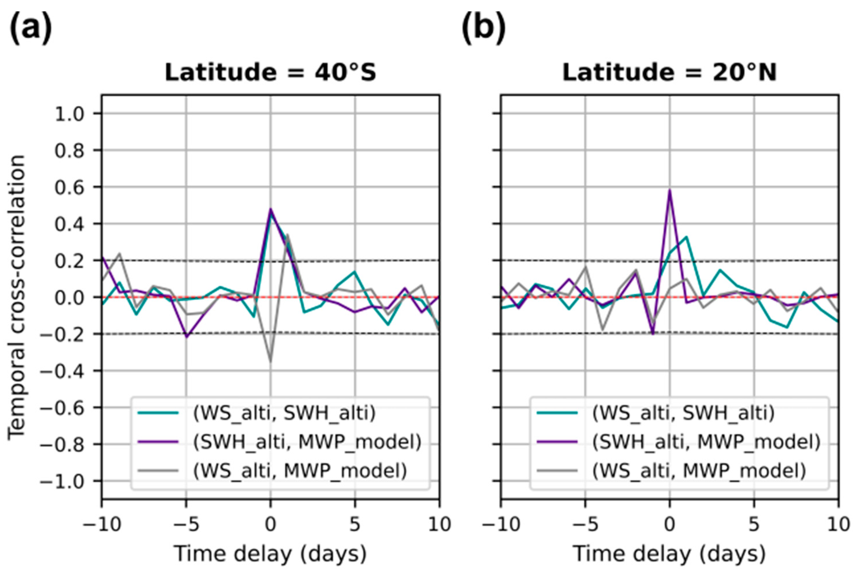
| −2 Days | −1 Day | 0 Day | +1 Day | +2 Days | |
|---|---|---|---|---|---|
| (WS_alti, SWH_alti) | 3.4% | 8.2% | 88.1% | 36.5% | 5.4% |
| (SWH_alti, MWP_model) | 4.6% | 7.9% | 89.7% | 43.5% | 5.1% |
| (WS_alti, MWP_model) | 3.4% | 6.8% | 72.7% | 45.7% | 7.8% |
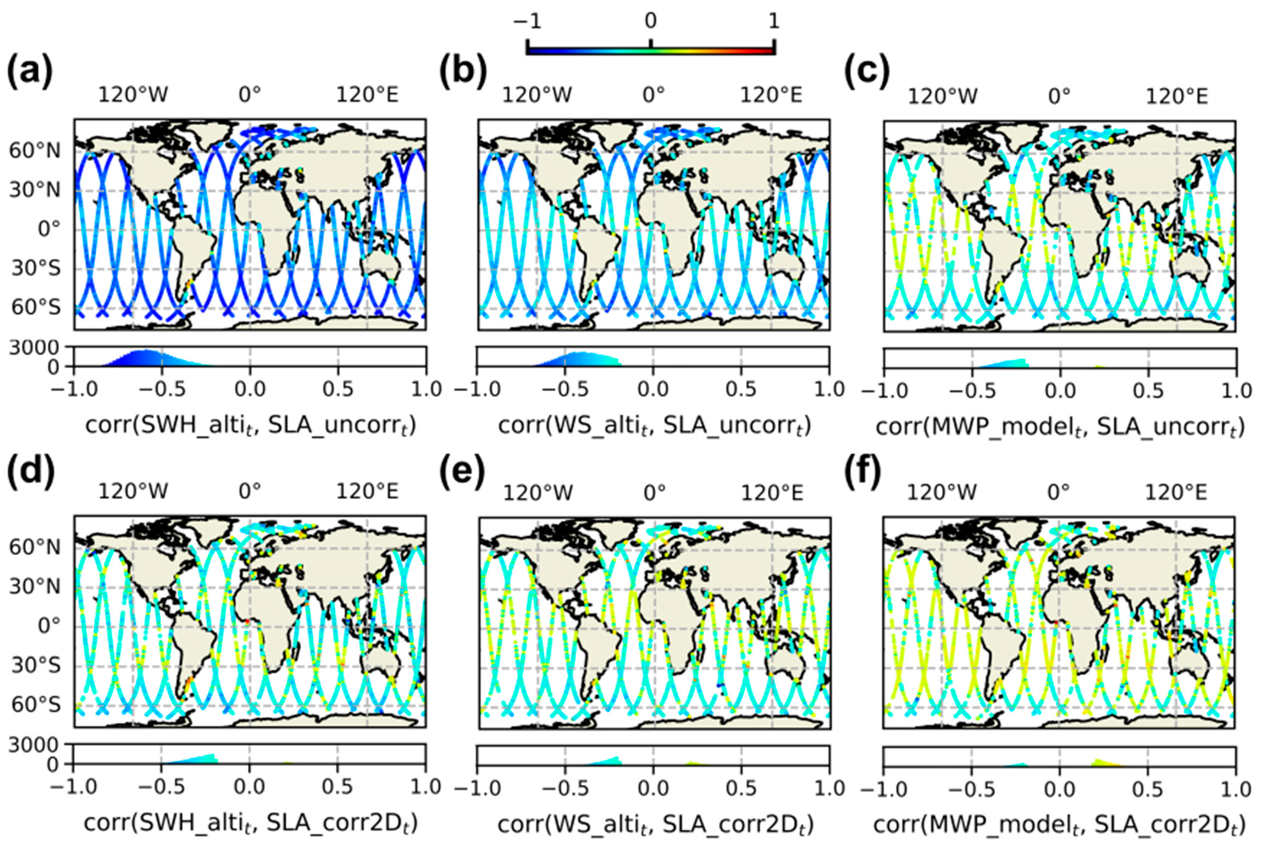
| −2 Days | −1 Day | 0 Day | +1 Day | +2 Days | |
|---|---|---|---|---|---|
| (SWH_alti, SLA_uncorr) | 6.2% | 9.9% | 98.4% | 7.6% | 6.2% |
| (SWH_alti, SLA_corr2D) | 6.1% | 10.9% | 31.8% | 10.7% | 7.9% |
| (WS_alti, SLA_uncorr) | 6.0% | 11.6% | 82.5% | 23.1% | 8.0% |
| (WS_alti, SLA_corr2D) | 5.9% | 7.3% | 23.4% | 10.2% | 7.4% |
| (MWP_model, SLA_uncorr) | 4.9% | 22.6% | 32.8% | 12.0% | 6.1% |
| (MWP_model, SLA_corr2D) | 5.4% | 10.2% | 22.0% | 8.5% | 6.7% |
Disclaimer/Publisher’s Note: The statements, opinions and data contained in all publications are solely those of the individual author(s) and contributor(s) and not of MDPI and/or the editor(s). MDPI and/or the editor(s) disclaim responsibility for any injury to people or property resulting from any ideas, methods, instructions or products referred to in the content. |
© 2024 by the authors. Licensee MDPI, Basel, Switzerland. This article is an open access article distributed under the terms and conditions of the Creative Commons Attribution (CC BY) license (https://creativecommons.org/licenses/by/4.0/).
Share and Cite
Mazaleyrat, E.; Tran, N.; Amarouche, L.; Vandemark, D.; Feng, H.; Dibarboure, G.; Bignalet-Cazalet, F. Analysis of High-Frequency Sea-State Variability Using SWOT Nadir Measurements and Application to Altimeter Sea State Bias Modelling. Remote Sens. 2024, 16, 4361. https://doi.org/10.3390/rs16234361
Mazaleyrat E, Tran N, Amarouche L, Vandemark D, Feng H, Dibarboure G, Bignalet-Cazalet F. Analysis of High-Frequency Sea-State Variability Using SWOT Nadir Measurements and Application to Altimeter Sea State Bias Modelling. Remote Sensing. 2024; 16(23):4361. https://doi.org/10.3390/rs16234361
Chicago/Turabian StyleMazaleyrat, Estelle, Ngan Tran, Laïba Amarouche, Douglas Vandemark, Hui Feng, Gérald Dibarboure, and François Bignalet-Cazalet. 2024. "Analysis of High-Frequency Sea-State Variability Using SWOT Nadir Measurements and Application to Altimeter Sea State Bias Modelling" Remote Sensing 16, no. 23: 4361. https://doi.org/10.3390/rs16234361
APA StyleMazaleyrat, E., Tran, N., Amarouche, L., Vandemark, D., Feng, H., Dibarboure, G., & Bignalet-Cazalet, F. (2024). Analysis of High-Frequency Sea-State Variability Using SWOT Nadir Measurements and Application to Altimeter Sea State Bias Modelling. Remote Sensing, 16(23), 4361. https://doi.org/10.3390/rs16234361