Abstract
Neuro-symbolic models combine deep learning and symbolic reasoning to produce better-performing hybrids. Not only do neuro-symbolic models perform better, but they also deal better with data scarcity, enable the direct incorporation of high-level domain knowledge, and are more explainable. However, these benefits come at the cost of increased complexity, which may deter the uninitiated from using these models. In this work, we present a framework to simplify the creation of neuro-symbolic models for tree crown delineation and tree species classification via the use of object-oriented programming and hyperparameter tuning algorithms. We show that models created using our framework outperform their non-neuro-symbolic counterparts by as much as two F1 points for crown delineation and three F1 points for species classification. Furthermore, our use of hyperparameter tuning algorithms allows users to experiment with multiple formulations of domain knowledge without the burden of manual tuning.
1. Introduction
Remote sensing is central to conducting efficient forest inventories on large spatial scales [1,2]. Making use of the large volumes of data produced by remote sensing requires automated tools. The fundamental tasks of processing remotely sensed data aim to answer two questions: Where are the trees, and what kinds of trees are they? These questions are addressed by crown detection (or delineation) and species classification tasks. While some forest parameters, such as leaf chemistry [3,4], can be estimated without identifying tree species, knowing the species identity of trees allows for improved estimates of size and carbon-related measurements as well as the ability to conduct biodiversity-based research and conservation [5,6].
Remote sensing-based tree crown delineation and species classification are inherently difficult problems. Crown boundaries can be hard to determine due to irregularly shaped crowns and overlapping adjacent crowns, especially in dense forests [7]. Depending on the resolution of the image, pixels that comprise the boundaries of trees may receive light from one or more tree canopies as well as light from nearby objects, understory vegetation, or the ground [8]. Mixed pixels also make species classification more challenging [9]. Species classification is also complicated by variations in crown traits, like leaf chemistry or crown leaf density, and their responses to environmental factors like soil nutrient or water availability [10,11,12].
Species may also have high spectral similarity to other species, for example from closely related species with similar shapes and crown densities [13,14]. The difficulty in separating species increases with the number of species in a forest. Generally, species classification accuracy tends to be inversely related to the number of species considered for classification [15,16]. Atmospheric contributions to the image, viewing geometry, and shadows make both delineation and species classification more challenging [17,18,19].
Machine learning algorithms such as deep learning models are the state of the art in automated forest inventory methods for both crown detection/delineation and species classification [20,21,22]. Deep learning models are statistical models with potentially billions of learned parameters, typically trained on labeled datasets. The performance of a deep learning model on a task tends to improve as the number of learned parameters increases, but the size of the dataset required for the model to be performant grows superlinearly with the number of model parameters [23,24].
Convolutional neural networks (CNNs) are some of the most commonly used models for image-based crown delineation and species classification [25]. These models typically contain on the order of millions of parameters and require large datasets for training, usually ranging from thousands to millions of images [23,26]. Amassing and labeling large datasets is typically one of the highest hurdles to creating a useful model [24].
Another frequently cited drawback of deep learning models is their lack of explainability [27,28]. These models are considered black boxes, where the reasoning behind their inferences cannot be easily determined by the user. In many instances, explainability is not required for the model to be useful, but there are situations where understanding the “why” of a model’s predictions is important, particularly for critical decisions and to gain insight into the problem being researched.
Symbolic models are models that represent real-world characteristics as variables linked by a series of operations. Common examples of symbolic models include logical formalism, such as propositional logic, first-order logic (FOL), and mathematical equations. Contrary to deep learning models, it is easy for a human to understand the reasons behind these models’ predictions; however, these models do not typically generalize well. Moreover, it is easy for humans to represent expert knowledge using logic formalisms, ensuring that the model captures high-level concepts.
Neuro-symbolic models are deep learning model-symbolic model hybrids that are more robust than either model on its own [29,30]. Neuro-symbolic models have been shown to perform well with reduced datasets, proving useful in zero-shot and few-shot learning scenarios, and function more transparently for the user [31]. Neuro-symbolic models also have the advantage of incorporating ecological knowledge into algorithms based purely on image data, analogous to how a field biologist uses their ecological knowledge—such as a habitat in which species are likely to occur—in addition to organismal features, to identify a species. This field of machine learning has been applied to several ecological problems. Xu et al. applied a neuro-symbolic approach to the fine-grained image classification of birds [32]. Sumbul et al. used a neuro-symbolic model for zero-shot learning in identifying tree species [33].
There are several mechanisms for creating neuro-symbolic models from deep learning models. Seo et al. used a regularization technique with a method similar to ensembling [34]. Hu et al. used posterior regularization and knowledge distillation [35]. Dilligenti et al. used a similar technique called semantic-based regularization (SBR) to create neuro-symbolic models [36]. In this work, we focus on SBR.
Semantic-based regularization works by adding a regularization equation in the form of a fuzzy FOL expression to the model’s loss function. Fuzzy FOL uses continuous functions as its operators, making it differentiable. This is a necessary property for loss functions in models trained using backpropagation and is employed by most neural models [37]. During training, the model is penalized for predictions that fail to satisfy the FOL encoded rule.
Although neuro-symbolic models are more robust, they also have their shortcomings. Turning domain knowledge into a rule or equation that can be incorporated into a machine learning model can be challenging, particularly for rules written in first-order logic. Once a rule is formulated in FOL, it must be written in a programming language, usually the same language used to program the neural model. Furthermore, after a rule is written, depending on the neuro-symbolic framework, there may be many hyperparameters that need to be tuned. Hyperparameters are model variables that are set by the user rather than learned [38]. The number of hyperparameters varies with the model used, but they usually number in the tens. Integrating FOL statements into the model introduces additional hyperparameters that must be tuned. Usually, each rule has its own hyperparameters. When multiple rules are involved, they may interact in unexpected ways, increasing the complexity of tuning. Selecting values for rule hyperparameters that work effectively is a time-consuming task.
In this paper, we introduce an SBR-based neuro-symbolic framework paired with hyperparameter tuning algorithms as one solution to alleviating some of the difficulties in creating neuro-symbolic models. Our object-oriented approach provides rule templates that enable users to quickly model rules in FOL using the inheritance paradigm of object-oriented programming. Our framework includes three hyperparameter tuning algorithms—random search, grid search, and Bayesian optimization—to ease the burden of finding optimum rule parameters [39].
Throughout the remainder of this paper, we describe the architecture of our framework and illustrate its use in two ecologically relevant scenarios: crown delineation and species classification. For the crown delineation model, we use DeepForest, a popular individual tree crown delineation model based on RetinaNet [40]. DeepForest is designed to detect tree crowns in remote sensing RGB images. To demonstrate a species classification use case, we use a model from reference [41], which is a well-cited paper by Fricker et al. The Fricker model can process both RGB and hyperspectral remote sensing data, but in this paper, we focus on RGB. We use data from the National Ecological Observatory Network to train each model [42]. For the crown delineation model, we use data from Niwot Ridge, an alpine forest in Colorado [43]. For the species classification model, we use data from the Tea Kettle Experimental Forest, TEAK, a mixed-conifer forest in California [44]. Although we use these models and data to demonstrate the use of our framework, the framework is model-agnostic and can be applied to any neural model that can be written in Python.
2. Framework Architecture
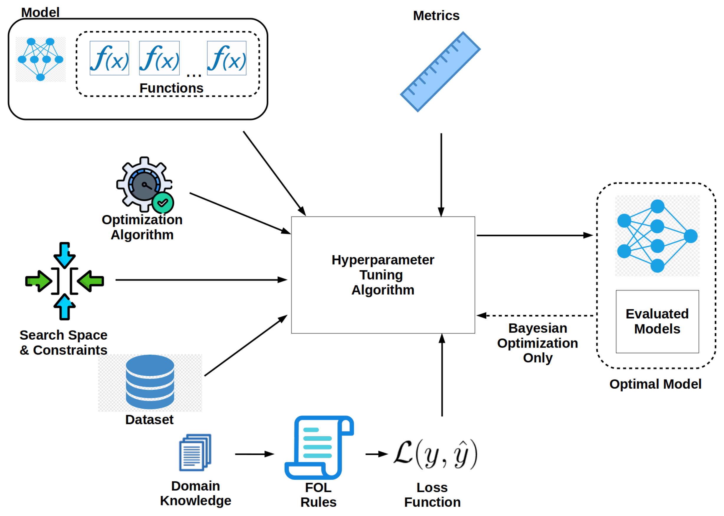
Our framework was written in Python version 3.11.6 primarily using PyTorch 2.0.1 and PyTorch Lightning 2.1.0 [45,46]. Meta’s Bayesian optimization package Ax version 0.3.4 was used for Bayesian optimization [47]. We created our models using PyTorch Lightning, whose predefined classes are easily extendable to any neural model. The code for our framework is available for download on GitHub at https://github.com/ihmn02/forest_ecology_neuro_symbolic_framework (accessed on 18 November 2024) and is released for general use under MIT licensing. The majority of our code was written using the object-oriented programming paradigm. The corresponding data used in each model is available from NEON at https://www.neonscience.org/data (accessed on 30 October 2024) and can be downloaded from Zenodo at https://zenodo.org/records/14194555 (accessed on 18 November 2024). A block diagram of the framework’s architecture is shown in Figure 1.

Figure 1.
Framework’s system overview.
3. User Workflow
We will touch upon the specifics of the framework as we go through an overview of the user workflow. There are four stages to the workflow: creating rules, modifying the original model and loss function, model tuning, and training and evaluation.
3.1. Creating Rules
First, the user must decide what rules they want to incorporate into the model. Each rule must be converted into an FOL statement, and each statement must be converted into an FOL object. In FOL, the simplest element of a statement is an atom. Atoms are composed of predicates or functions and their terms. Terms are the arguments of the functions or predicates. Predicates return only true or false, while functions can return any value within a specified range. We will build our atoms using functions. These functions, contained within the statements, may be networks from the deep learning model or defined by the user. Probabilistic FOL operators such as AND, OR, NOT, and IMPLIES are used to connect functions, forming a meaningful rule.
Probabilistic FOL operators are continuous and have a range of [0, 1] unlike normal binary operators, which are discrete [48]. Because the operators are continuous and differentiable, they do not break the backpropagation algorithm used to train the neural networks [37]. See [48] for an introduction to probabilistic FOL.
Starting with natural language, most concepts can be converted into FOL. The simplest and most common statements take the following form:
This formula reads as follows: for all x, P of x implies Q of x, where P and Q are functions of x. For example, suppose the user is training a species classification model on RGB and LiDAR data from a mature forest containing two species of trees—red maples and white pines. The user knows that in this forest, all red maples have a crown height of 40 meters or less, so any trees taller than 40 meters must be white pines. The user can write an FOL statement for this rule as follows:
where x is an RGB instance from the dataset with its corresponding CHM. and are functions, in this case, neural networks that predict a real number between 0 and 1 for a given instance from the dataset. A tree much taller than 40 m would produce a prediction near 1 and a tree less than 40 m would produce a prediction closer to 0. If the instance is white pine, the function should predict a value close to 1, otherwise, it should predict a value close to 0.
Atoms can be linked by operators. In probabilistic FOL, there are several implementations of operators, but in all cases, the operators are implemented as functions. In this work, we use the Łukasiewicz t-norm version of the operators given in Table 1 [49].

Table 1.
Łukasiewicz operators and their implementation.
The truthfulness of an FOL expression is then calculated by substituting the output from each function into the FOL operator and then evaluating the expression. The process of assigning values to the terms of an FOL expression is called grounding. A true expression will evaluate to 1 and a false expression to 0. An expression can have any value between 0 and 1. Using the Łukasiewicz t-norm, the example rule is evaluated as follows:
Each rule is assigned a real number that represents the importance of the rule.
Our framework provides templates for basic FOL expressions. These templates are classes that the user can modify to fit their needs using inheritance. There are templates for rules of the following forms: , , , , , and . The rule classes have methods for each FOL operation and an eval method to evaluate the rule. The atoms of the expression are the arguments of the eval method. The rule objects include a generic_interface method to simplify linking the model and the rule object. In the generic interface, the user should create variables that map the predictions from the model to named variables in the rule object. Table 2 lists the name of each class and its expression. Classes for new expressions can be added using inheritance.

Table 2.
Predefined expression classes and their corresponding FOL.
3.2. Modifying the Original Model and Loss Function
Assuming that the user has an existing deep learning model that they want to make neuro-symbolic, the next step involves model modification. Continuing with the example from Step 1, let us assume we have a classifier capable of identifying tree species from RGB images as our original model. We will call the RGB image and its corresponding label .
There are many ways to create neuro-symbolic models from vanilla deep neural networks; one of the most straightforward is semantic-based regularization. That is the method we use in this paper. As the name implies, SBR adds rules written as statements of FOL to the model’s loss function. See [36,50,51] for a more comprehensive discussion of SBR.
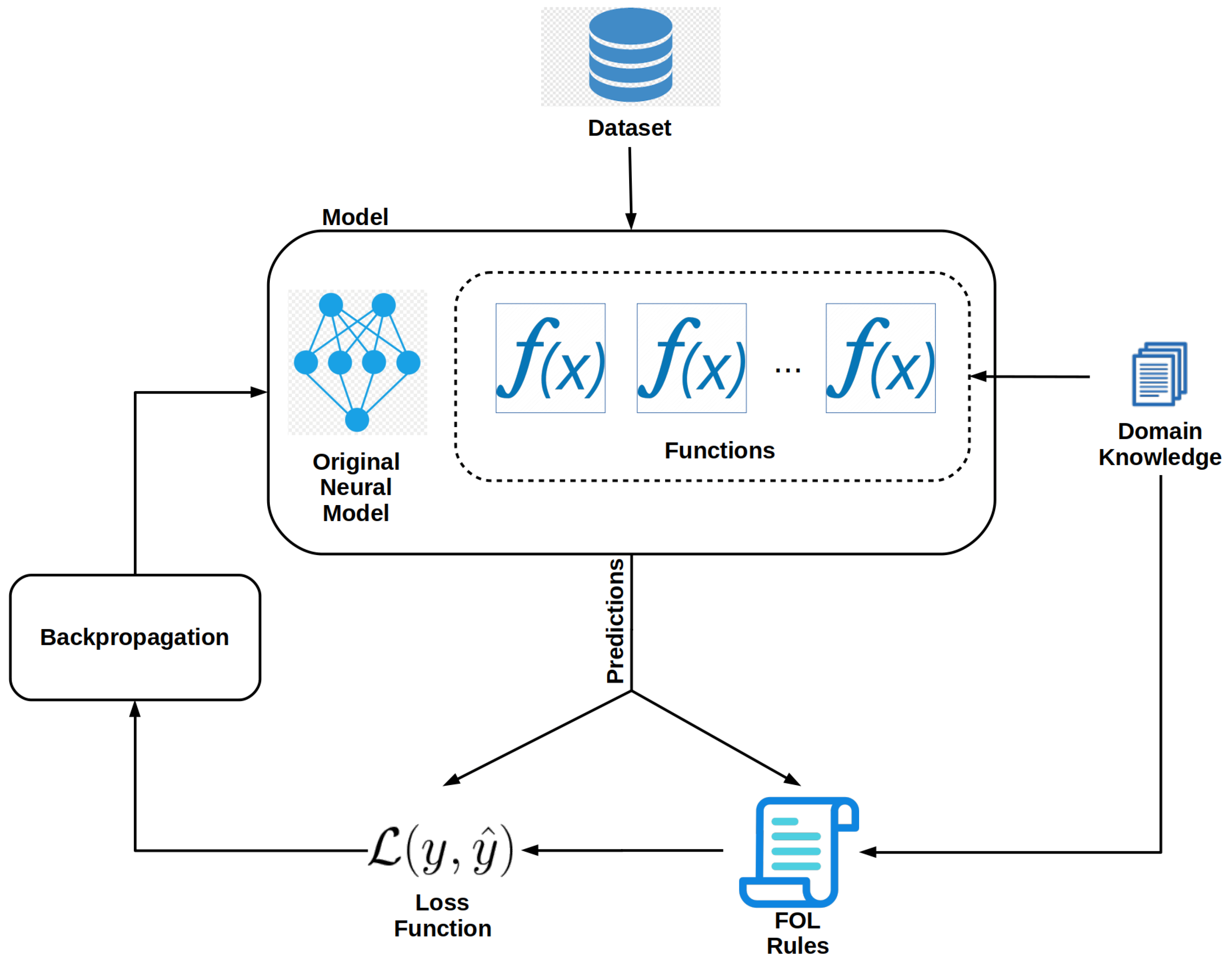
Functions that make up the atoms of an FOL expression must be added to the model. These functions can be learned or user-defined [36]. In this work, we use user-defined functions but learned functions can be readily used with our framework. Each new network is designed to perform a specific task such as identifying trees that have a crown height of greater than 40 m. The addition of the learned functions effectively turns the model into a multi-task learning deep neural network. Figure 2 shows a diagram of a modified model and the training process. In the diagram, functions are added to the original network, and their predictions are used in the FOL expressions. The user can arbitrarily add many functions. In the case of our toy example, the dataset would need to be augmented with the CHM model aligned with the RGB images. This can be done by appending a CHM raster of the same width and height to the RGB image as an additional layer.
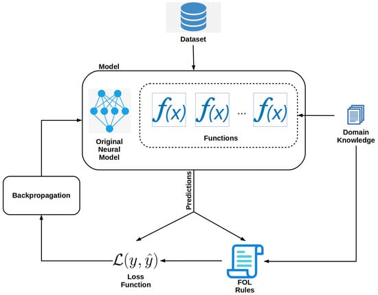
Figure 2.
Model modifications needed to create a neuro-symbolic model.
How new networks are added to the model depends on model implementation. In the code provided, we use the PyTorch Lightning LightningModule class as the backbone of each model. Then, new networks are added using PyTorch’s nn.Module class. A description of its use can be found in [52]. There are no restrictions on the architecture of the additional networks. However, the output of the final layer must be a real number between 0 and 1 or must be able to be decomposed into a real number between 0 and 1 if the output has more than one dimension.
New loss terms must be added to the original model’s loss function. Loss terms must be added for the new networks. A loss term must also be added to complete the SBR implementation. The additional term penalizes the model if it fails to make predictions that make all rules true. We’ll use the notation from [51]. The SBR loss term takes the following form:
where H is the number of rules, denotes the user-assigned importance of rule , denotes the average evaluation of rule h when grounded using the data in the training batch, and f denotes the set of functions comprising the following rules:
For our example, rule is as follows:
and x denotes the grounding of the argument for each function for all values in a training batch. The final loss function should have the following form:
where denotes the typical loss, which includes terms for loss from networks and regularization, and the summation term is the loss incurred from the SBR rules.
3.3. Model Tuning
Hyperparameter tuning is the selection of values for the model’s non-learned parameters. The values selected can have a heavy impact on the model’s predictive performance, training time, and other performance measurements. Once the model and loss function are updated, the hyperparameters can be tuned. The process is usually conducted on a validation set—a set of hold-out data separate from the test and training set. To begin the tuning process, the user must decide what variables to tune. Neural networks typically have many hyperparameters such as the learning rate, an L2 regularization constant, and the number of layers used in the network. Because the focus of this work involves the creation of neuro-symbolic models, we focus on the hyperparameters that relate to the rules, in our case . After a variable is selected, the user must define the upper and lower bounds of the search space. Selecting bounds is usually done through a combination of intuition and trial and error. Once the user decides on bounds for the search space, one or more metrics must be chosen to gauge the model’s performance as the search parameters are varied. Common metrics include F1, accuracy, and total loss. The user also selects an optimization algorithm such as the Adam optimizer or plain stochastic gradient descent. The optimizer selected will also be used during the training process. Searching through the parameter space is an iterative process. Each iteration is known as a trial. The user decides the number of trials to run prior to starting the hyperparameter tuning algorithm. Our framework includes three algorithms for hyperparameter tuning, random search, grid search, and Bayesian optimization. Random search randomly selects points within the search space with a uniform distribution. Random search is shown to provide good results, especially for high-dimensional search spaces, which require a great deal of time to train. Random search provides near-optimum results with as few as 60 trials [53].
Rather than picking random points within the search space, grid search searches the space systematically using an even spacing between search points. The granularity of the search is determined by the number of trials.
Unlike random search and grid search, Bayesian optimization is a closed-loop search algorithm; the results of previous trials are used to choose the next points for evaluation. The algorithm attempts to learn which areas of the search space are likely to provide optimum results. Bayesian optimization requires at least 50 trials or more to work well. As the volume of the search space grows, more trials are needed to produce good results. See [54] for a detailed explanation of Bayesian optimization.
After selecting the desired tuning parameters, the model is evaluated for the indicated number of trials. After the last trial, a sorted list of the chosen model parameters and their associated performance is printed in descending order and saved to a CSV file.
3.4. Training and Evaluation
The user can manually enter the best hyperparameters found in the previous step prior to training and testing the model on the test set.
4. Use Cases
4.1. Individual Tree Crown Delineation
We demonstrate the use of our framework for crown delineation using DeepForest, a popular open-source crown delineation model based on RetinaNet, a CNN [40,55]. Using our framework we will do the following:
- Create two rules.
- Modify the model and loss function to use SBR.
- Find optimum values for the rule lambdas.
- Evaluate the effectiveness of each rule.
We trained the model on data from Niwot Ridge (NIWO), an alpine forest in Colorado, USA. Niwot is located at a latitude of 40.05425º and a longitude of −105.58237º. Its mean annual precipitation is 1005 mm and the mean annual temperature is 0.3 °C. The site elevation ranges from 2975 m to 2583 m. The tree canopy cover varies from continuous at lower elevations and on south- and east-facing slopes, to open forests with isolated trees at higher elevations. Understory coverage is limited, especially at higher elevations. The mean canopy height is 0.2 m (all canopy height values listed here include bare ground, and the prevalence of bare ground at Niwot Ridge is why this value is so small). The dominant tree species are conifers, primarily lodgepole pine, subalpine fir, and Engelmann spruce [43,56].
4.1.1. Data
The data were collected in 2018 by the National Ecological Observatory Network (NEON). NEON is a program funded by the US federal government and is tasked with monitoring environmental health at over 80 sites across the continental United States, Alaska, and Puerto Rico [42]. Part of their mission is to monitor forest health, carbon fluxes, and biodiversity changes through field surveys and remote sensing. NEON annually overflies forests located at their sites during periods of peak greenness using their Airborne Observation Platform (AOP) [42]. The NEON AOP is an aircraft outfitted with RGB, hyperspectral (HSI), LiDAR, and GPS sensors. The HSI data have a resolution of 1 m and RGB imagery data have a resolution of 0.1 m. The canopy height model (CHM) data produced by the LiDAR sensor has a spatial resolution of 1 m2 per pixel. NEON’s hyperspectral data are atmospherically corrected and all data are orthorectified and aligned to a uniform spatial grid.
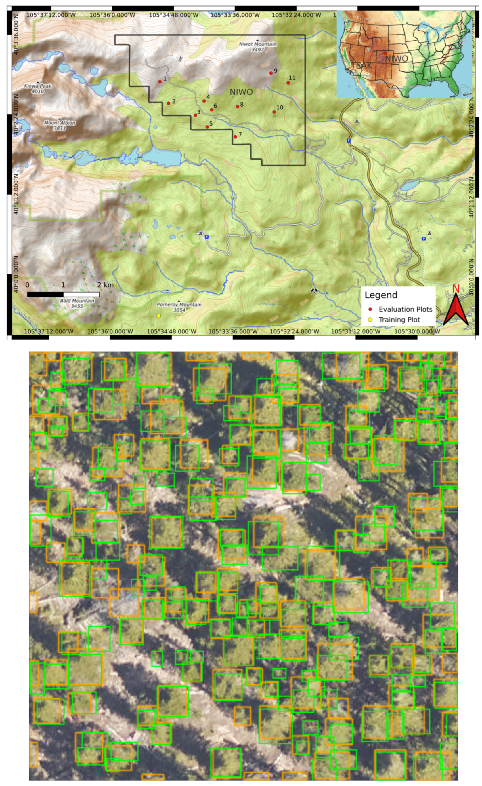
We trained our crown delineation model using a combination of RGB and CHM data. The original data were sourced from NEON’s L3 data products, specifically 1 km2 mosaicked tiles. We decomposed rasters larger than 500 pixels in any dimension down to 400 × 400 pixels or less rasters with 5% overlap. A map showing the geolocation of the training and evaluation plots used is shown in Figure 3.
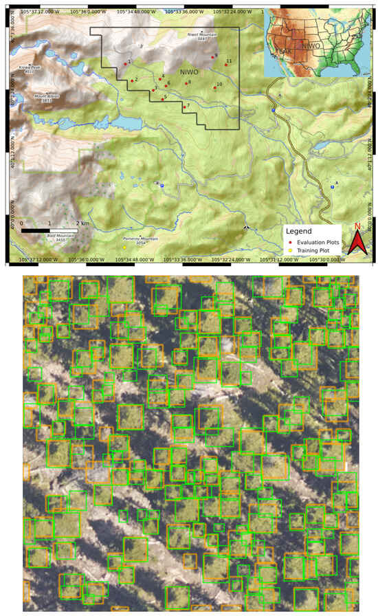
Figure 3.
(Top) A map of the geolocations of plots used in the training and test sets at Niwot. Red dots indicate the locations of plots used for the test set, while the yellow dot marks the location of the plot used for the training set. The black boundary outlines the extent of NEON’s sampling area for the NIWO site. (bottom) Ground truth and DeepForest predicted bounding boxes for plot number 8 at NIWO after training the model with optimal rule parameters found using random search. The ground truth bounding boxes are depicted in green, and the DeepForest predictions are in orange.
An example evaluation plot is shown in Figure 3 (bottom). Each evaluation plot is 400 × 400 pixels or has an area of 1600 m2. The number of trees per evaluation plot ranges from 5 to 292. The training plot is 2511 × 4132 pixels with an area of 103,975 m2. The plot has 12,412 trees. See [57,58] for a detailed description of the data collection and preparation methodology.
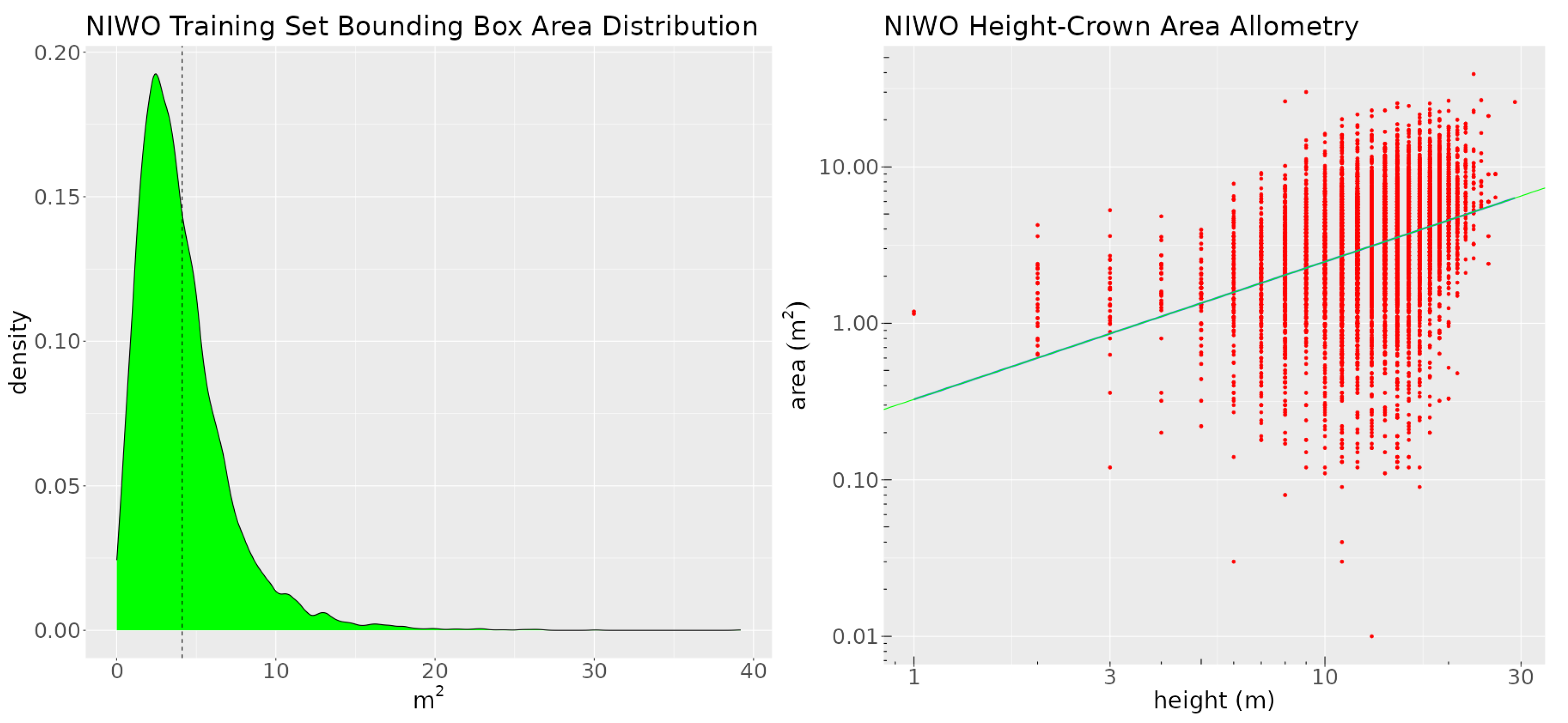
The dataset contains a single class—tree. We split the data into training, validation, and test sets. The sizes of these sets are 10,757, 1655, and 1624 annotations, respectively. The distribution of the crown area (derived from the crown delineations) and the height-crown area allometry (the relationship between each tree’s crown area and its height, derived from the canopy height model) are shown in Figure 4.

Figure 4.
The left image shows the crown area distribution of the training set at Niwot Ridge. The dashed black line is the mean of the distribution. The right image is a plot of the height-crown area allometry for the Niwot training set. The green line denotes the fitted log-linear height-crown function.
We will use the information contained in these graphs to craft two rules for the site. We appended the CHM rasters as a fourth layer to the RGB images. The training data were augmented using geometric transformations.
4.1.2. Creating Rules
DeepForest delineates crowns using rectangular bounding boxes. These bounding boxes are sometimes larger than the crowns of the trees they detect, which may reduce the performance of the model. We will create rules intended to reduce DeepForest’s tendency to use oversized bounding boxes. We will use two of the rules developed in [58]. As shown in Figure 4, the mean ITC area at Niwot is 400 pixels, which corresponds to approximately 4 m2. The distribution is right-skewed, with 60% of the crowns being smaller than the mean. Based on this observation, we formulated the following rule: a detected object is classified as a tree if and only if the area of its bounding box is less than 4 m2. Despite the use of if-and-only-if, the rule is not as strict as it sounds in natural language. We can control how strictly the rule is enforced by varying the value of the rule’s lambda. This allows us to use a simple rule like this even though we know that there are trees with crowns > 4 m2. We also create a second rule, similar to the first, more tightly related to how we think about limits on crown area biologically, by using the height-crown area allometry model shown in Figure 4. As described in [59,60], we fit a power function to map the height to the crown area for the trees at Niwot and use the CHM to predict the crown area given the crown height. We use the predicted crown area to create the following rule: a detected object is a tree if and only if its bounding box area is less than or equal to the area predicted by the crown height allometry model. We apply both rules at the same time and use the results of our evaluation to choose the better rule. In order to implement each rule, we create two user-defined functions. The first function quantifies how much the bounding box area for a detected object deviates from the site mean. If a bounding box is less than 400 pixels the function’s output tends toward 1. If the bounding box of a detected object is greater than 400 pixels, its output tends toward 0. We use the sigmoid function to ensure differentiability and write the function as follows:
where is DeepForest’s predictions for x, and is a function that calculates the area of a prediction’s bounding box. For Niwot, our fitted power function for the height-crown area allometry is as follows:
To create our second function, we substitute the site mean area with to give the following:
We use the function to extract the maximum value of the CHM for prediction . We rename our functions to make the FOL more intuitive. Let be . Let be . Let be . Using the functions, we can write our rules in FOL as follows:
and
4.1.3. Model and Loss Function
DeepForest is built from RetinaNet [40]. RetinaNet is a deep CNN with a feature pyramid network for scale invariance, a specialized loss function, and residual connections between layers. The network has 32.1 million learned parameters [55]. RetinaNet is well-suited for object detection. The network predictions include bounding box coordinates for detected objects as well as the object’s class. To complete the model, we add the additional terms to the loss function as described in Section 3.2. As in [58], we delay the application of the rules to the latter epochs of training to give the model time to learn purely from the dataset. We accomplish this by multiplying the rule loss by a function as follows:
where and are constants < 1, t denotes the training step number, and is a constant that controls at what steps the rules are applied. The loss function then becomes as follows:
where denotes the summation of all the loss terms, denotes the total standard loss, and denotes the sum of the loss from all rules. This method was chosen empirically to improve model performance [35].
4.1.4. Hyperparameter Tuning and Training
Let and be the hyperparameters associated with rules 1 and 2, respectively. We optimized the values of and to achieve the best F1 score on the validation set. We set the bounds for each to be between 0.01 and 9.0. Empirically, large values of tend to degrade model performance. All model hyperparameters are shown in Table 3.

Table 3.
Crown delineation model hyperparameters and species classification model hyperparameters for tuning.
To define F1 for an object detection model, first, we define the intersection over the union score or IoU. IoU is used as a measure of overlap between two bounding boxes. Given bounding box A and bounding box B, an IoU of 0 represents no overlap and an IoU of 1 represents full overlap. IoU is calculated as follows:
For a DeepForest prediction to be counted as a true positive (TP), the prediction must overlap a ground truth bounding box with an IoU of . Prediction bounding boxes that fail to meet this requirement are counted as false positives (FPs). If a ground truth bounding box does not have a matching prediction, it is counted as a false negative (FN). Using these definitions, we define precision as follows:
and recall as follows:
Then, F1 is as follows:
We tuned the model using three search algorithms: Bayesian optimization, grid search, and random search. We used the default settings for Bayesian optimization from the Ax package. We allowed 64 trials for each algorithm. Since model initialization produces variation in the results, we seeded the random number generator with 15 different seeds and reported the average of the results. The model was tuned and trained on one node of a high-performance computing cluster, using 16 GB of RAM, one NVIDIA A100 GPU, and one CPU.
4.1.5. Results
All three search algorithms improved the model’s performance over the non-neuro-symbolic model. The average change in F1 score for each model in comparison to the non-neuro-symbolic version of DeepForest is shown in Table 4. Bayesian optimization and grid search gave nearly identical results, improving F1 by approximately two F1 points. Random search gave the best result, improving model performance by 2.14 F1 points.

Table 4.
Average change in the test F1 compared to the non-neuro-symbolic model.
The bottom image in Figure 3 shows an example output of the model after training using optimal rule hyperparameters found using the random search algorithm. Ground truth bounding boxes are in green and the model’s predicted bounding boxes are in orange.
Figure 5 shows a density map of the points in the search space selected by each search algorithm. The figure highlights the differences in the search algorithms’ strategies. Bayesian optimization attempts to focus its search on areas of the plane that are likely to give optimum results, as can be seen by the high point density in the region near the axis of its graph. Grid search evenly distributes its points across the plane and random search chooses points at random, as reflected by the graph’s lack of structure.

Figure 5.
Contour plots of the points selected by each algorithm for all seeds.
Despite the differences in the search strategies, the rate of improvement as a function of trial number did not significantly vary between methods. As shown in Figure 6, after 29 trials, each method was within 0.5 points of the validation F1’s maximum range, suggesting that all the search algorithms were able to find optimum parameters with as few as 29 trials.
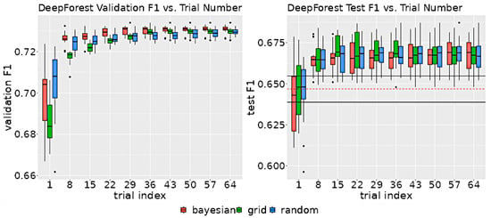
Figure 6.
The left graph displays the distribution of validation scores as a function of the number of trials for each search method. The right graph illustrates the distribution of test F1 scores, also as a function of the number of trials for each method. The test F1 score was determined by evaluating the model on the test set, using the hyperparameters associated with the highest validation score at the specified trial index. The black horizontal lines on the test F1 graph indicate the upper and lower 95% confidence intervals for non-neuro-symbolic DeepForest. The dashed red line denotes the mean test set F1 score of the non-neuro-symbolic model.
Figure 7 shows a plot of the validation F1 scores as a function of the rule lambdas. The plot indicates that optimum results are achieved when is near zero. This suggests that represents the more effective of the two rules tested.
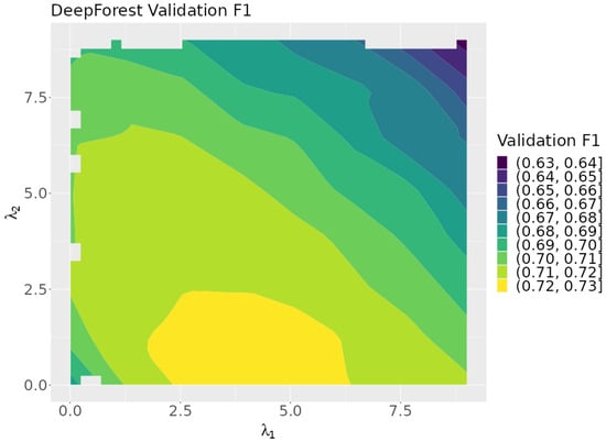
Figure 7.
A contour plot of the validation F1 scores over the search space.
5. Tree Species Classification
To demonstrate the use of our framework for a tree species classification use case, we conduct the following:
- Create two rules.
- Modify a tree species classification model and loss function for SBR.
- Find optimum values for the rule lambdas.
- Evaluate the effectiveness of each rule.
We use the model and data from [41] and two rules developed in [61]. The data are from TEAK, a mixed conifer forest in California USA close to the Nevada border. TEAK is located at a latitude of 37.00583° and a longitude of −119.00602°. It has a mean annual precipitation of 1223 mm and a mean annual temperature of 8 ºC. The average canopy height is 35 m. The elevation ranges from 2086 to 2734 m. The dominant tree species are red fir, white fir, Jeffrey pine, and lodgepole pine. Sixty-five percent of the study area is mixed conifer forest. The remaining area is covered by regions dominated by a single species, specifically red fir or lodgepole pine. Forest structure varies from closed-canopy forests to open stands with isolated trees. Understory density ranges from none at higher elevations to dense understory in some lower elevation areas. Citation [41] provides more information on the site.
5.1. Data
The remote sensing data were collected in 2017 by NEON. NEON surveys its sites annually during periods of peak greenness. Like the data used for crown delineation, the HSI data have a resolution of 1 m and RGB imagery data have a resolution of 0.1 m. The canopy height model produced from the LiDAR data has a spatial resolution of 1 m2 per pixel. The NEON remote sensing data were augmented with field survey data collected by the authors of [41] using sites established by [62]. NEON’s HSI data are atmospherically corrected and all data are orthorectified and aligned to a uniform spatial grid. See [41] for a more detailed summary of the data collection and preparation methodology.
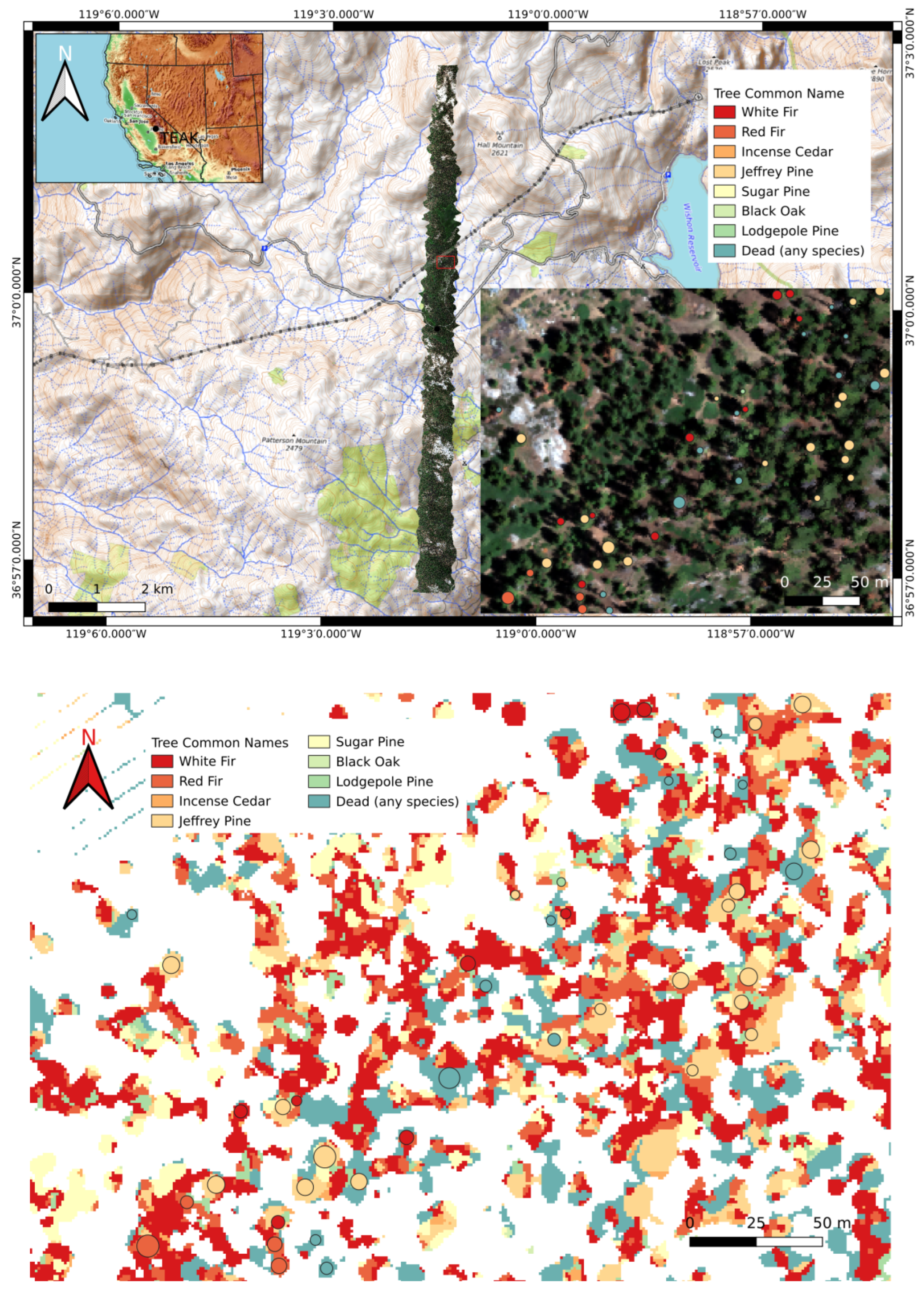
In this work, we used RGB and CHM data for species classification, although HSI data are more often used for this task. RGB data are more readily available outside of NEON sites, and the RGB-based classification is more prone to errors, allowing for a better demonstration of our methods. Nevertheless, our methods are applicable to HSI data as well. The dataset contains eight classes: white fir, red fir, incense cedar, Jeffrey pine, sugar pine, black oak, lodgepole pine, and dead. The dead category is composed of standing dead trees of any species. The top image in Figure 8 shows a map of TEAK and the bottom image shows a plot where tree species are identified.
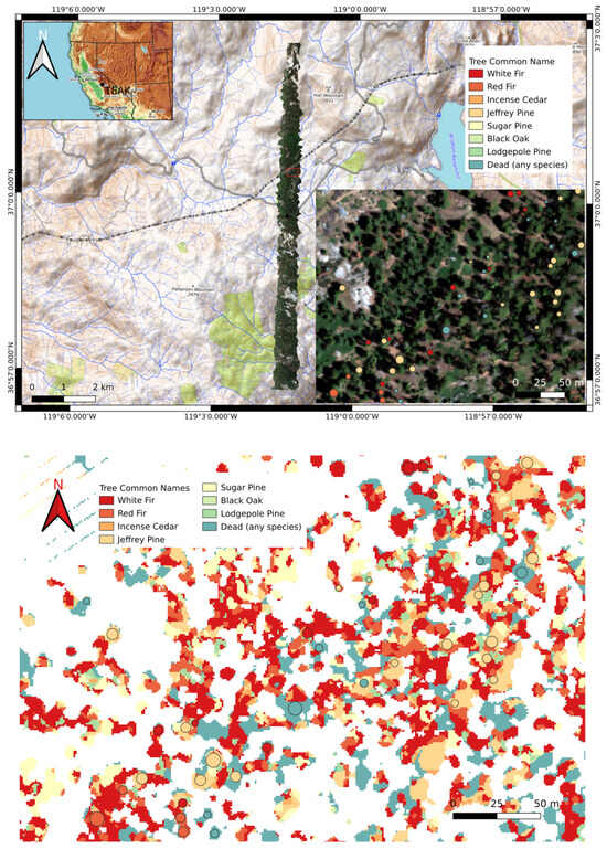
Figure 8.
(Top) A map of TEAK. The zoomed-in region in the lower right corner shows ground truth tree species labels. (bottom) Model predictions for the zoomed-in region above were generated using optimum hyperparameters found using the random search algorithm. Ground truth crown locations (from [41]) are indicated by circles. Colors within the circles are ground truth species identities.
Crowns from each tree were broken into patches of 15 × 15 pixels. Geometric transformation data augmentation was used to increase the size of the training set using the following transformations: horizontal flips, vertical flips, and 90-degree rotations. Table 5 shows the number of trees and pixel patches of each class.

Table 5.
Dataset tree crown and patch count by tree species.
We append the CHM raster to RGB images as a fourth layer. The CHM is removed prior to passing the data through the main network. Post data augmentation, we create a training set composed of 111,355 patches, a validation set of 12,373 patches, and a test set of 1796 patches. The test set patches were not augmented. Figure 9 shows the distribution of tree crown heights in the training set for each species. We will use this information to craft two rules.
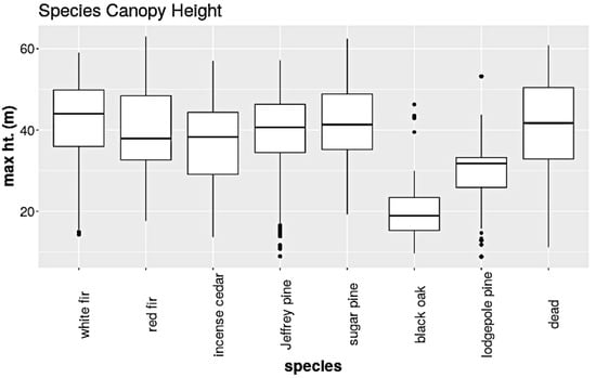
Figure 9.
The box and whisker plot of the crown height distribution for each species. Note that black oak and lodgepole pine are the shortest species.
5.2. Creating Rules
We will use the observed crown heights to help improve the model’s overall performance. We extend rules 1 and 2 from [61], which are based on the differences in crown height distributions. Rule 1 states that trees taller than 46.0 m are unlikely to be black oak. Rule 2 states that trees taller than 53.2 m are unlikely to be lodgepole pine. Note from the distributions that the majority of black oaks are less than 46 m in height and the majority of lodgepole pines are less than 53.2 m. We implement these rules by first creating our functions:
and
Both and are built on the sigmoid function, so both are differentiable. For , when the CHM values of x are less than 46.0 m, the output of the function tends toward 1, and when the values of x for the CHM are greater than 46 m, the output tends toward 0. We rename and to make our FOL more readable. Let be and let be . We then implement our rules in FOL as follows:
and
The functions and come from the original classifier whose function we will call . We use the components of the original classifier’s final prediction that correspond to the indices of the black oak and lodgepole pine classes respectively.
5.3. Model and Loss Function
The model comes from [41]. It is an eight-layer fully convolutional neural network with a softmax output layer. It has 684,000 learned parameters. We modify the loss function by adding a term for the rule loss as described in Section 2.
5.4. Hyperparameter Tuning and Training
The hyperparameters associated with rule 1 and rule 2, and , respectively, are the variables we tuned the model on. Table 3 shows all hyperparameter values used to tune the model. The choice of search space bounds was conducted through intuition. Large values for rule lambdas tended to worsen model performance. Model performance was found to vary with model initialization; therefore, we ran the experiment 10 times, each time initializing the random number generator with a different value and averaging the results. The scale variable was set arbitrarily to 1.0. We ran separate sets of 10 trials of 64 using all 3 search algorithms for comparison. When tuning for a production model, this need not be the case. We chose the validation macro F1 score to compare results across trials. We define F1, precision, and recall in Section 4.1.4, where TP is the number of true positives, FP denotes the number of false positives, and FN denotes the number of false negatives. We report the performance of the tuned model using the test set macro F1 score. The model was tuned and trained on one node of a high-performance computing cluster using 16 GB of RAM, 1 NVIDIA A100 GPU, and 1 CPU.
5.5. Results
As shown in Table 4, all three search methods found parameters that improved the model’s performance compared to the non-neuro-symbolic model. Again, the random search algorithm achieved the largest improvement with 3.02 F1 points. Bayesian optimization fared second best with 1.11 F1 points, and the grid search algorithm only found parameters that improved the model by 0.8 F1 points. The bottom image in Figure 8 shows the predicted species for the zoomed-in region at the top of the figure. The circles indicate ground truth labels.
Figure 10 shows density plots of the points selected in the search space by each algorithm. The Bayesian optimization algorithm focused its search heavily on the lower right corner of the search space. Grid search points were evenly distributed throughout the space. The random search algorithm points show no recognizable pattern.

Figure 10.
The density plots of the points selected by each search algorithm.
Figure 11 shows the distribution of the model validation set and test set F1 scores as a function of the number of trials. The median of the validation distribution for all 3 algorithms increases up to 8 trials and remains relatively flat after 43 trials.
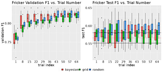
Figure 11.
The left graph shows the distribution of the validation F1 scores for the indicated number of trials for each search algorithm. The right graph shows the distribution of test F1 scores for the indicated number of trials. The hyperparameters selected for the test model were the ones corresponding to the highest validation F1 score up to the indicated trial. In the test graph, the two horizontal black lines indicate the 95% confidence intervals for non-neuro-symbolic test set F1 scores. The horizontal dashed red line indicates the mean of the non-neuro-symbolic model test set F1 scores.
The Bayesian optimization model improved at a faster rate than the other two algorithms. There was a great deal of overlap between the test set F1 scores for the non-neuro-symbolic model and the neuro-symbolic model due to the small improvement in performance from the rule implementation that is roughly of the same order as the model variance.
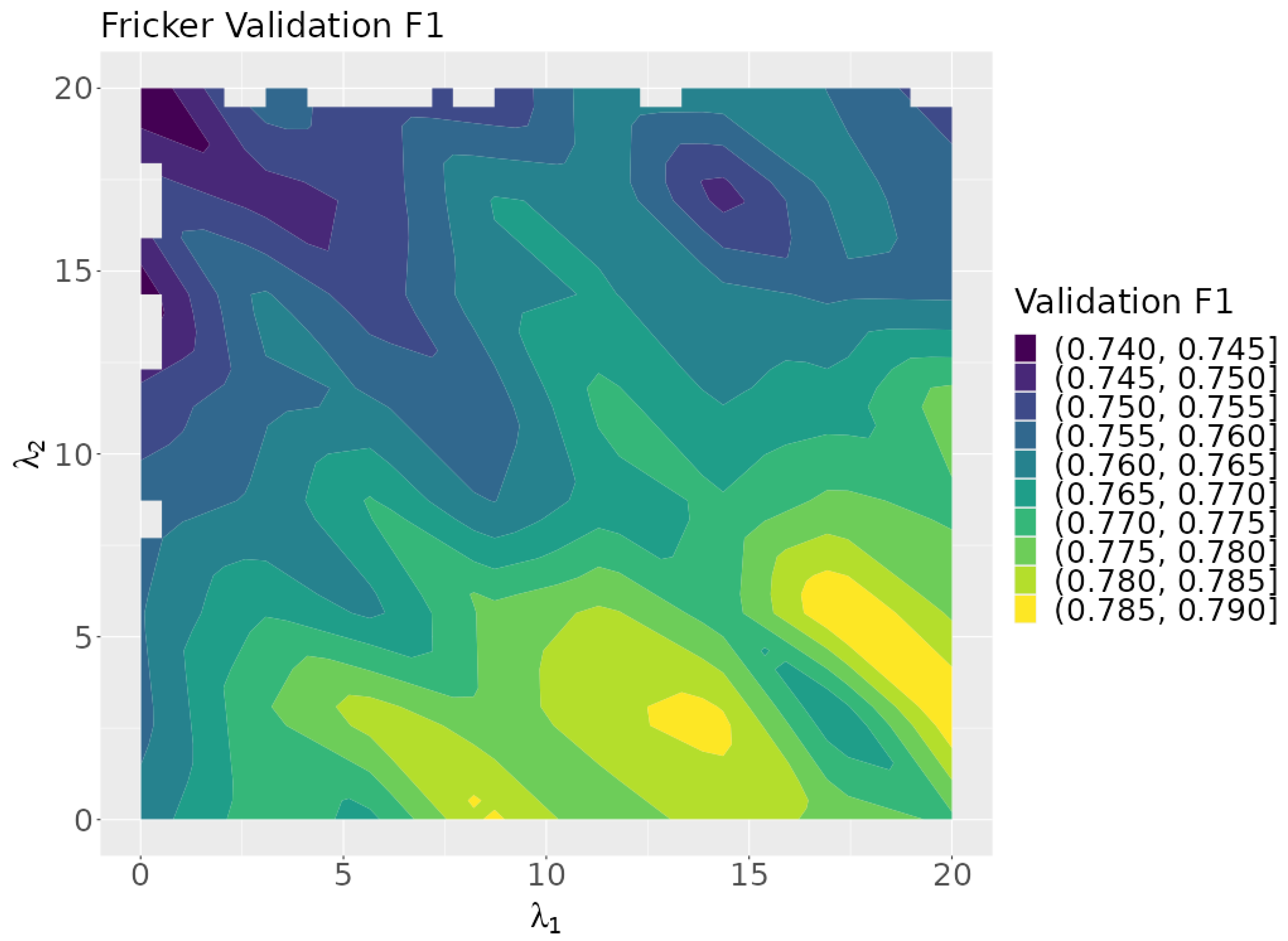
Figure 12 plots the neuro-symbolic model’s validation F1 scores over the rule lambda search space. Larger values correspond with higher validation scores, suggesting that rule 1 is more impactful than rule 2. This is surprising since rule 1 is for the black oak class, which has the fewest number of instances in the dataset. The highest validation scores are concentrated in the lower right corner of the search space, which corresponds to the area focused on by the Bayesian optimization algorithm.
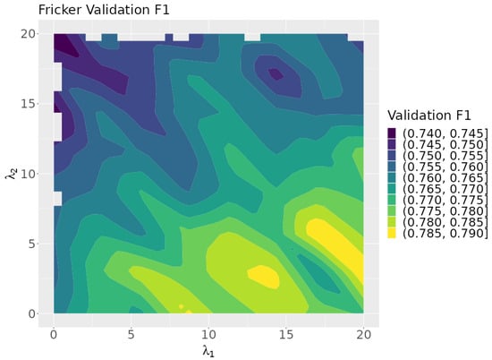
Figure 12.
Validation F1 as a function of and .
6. Discussion
We explored the application of our neuro-symbolic framework to crown delineation and species classification. The use of the neuro-symbolic framework increased the accuracy of both crown delineation and species classification over non-neuro-symbolic deep learning algorithms. The increase was modest but found for all four rules that were used. This indicates that knowledge about tree crown size and height-crown area allometry, translated into simple rules, can improve crown delineation from image data alone. In addition, simple formulations about the heights of co-occurring canopy species can improve species classification. Additional rules developed from ecological knowledge, such as which species are likely to co-occur together or at different elevations, may further enhance model performance and be tailored to local ecological contexts. Ecological knowledge about natural forests may be translated into FOL rules, although the benefit in classification accuracy of adding these rules needs to be tested more broadly across more forest types, including closed-canopy broadleaf forests. In addition, specific knowledge about management, such as planting spacing, could potentially generate useful rules in plantation forests. The four rules that we demonstrated cover the formulation that domain knowledge is likely to take when converted into FOL, using implication and if-and-only-if clauses. However, more complex rules may require more creativity on the part of the user to implement. Nevertheless, the tools needed to express more complex ideas are present within the framework.
Additionally, we demonstrated the use of three hyperparameter tuning algorithms to find optimal rule parameters. All three algorithms were able to find sets of parameters that improved the neuro-symbolic models’ performance over the baseline model. Parameters found by the random search algorithm outperformed those found with Bayesian optimization and the grid search algorithm for both models explored. No method was consistently more efficient than any other, which is surprising due to the closed-loop nature of the Bayesian optimization algorithm. Our results are partially in line with the findings of [53].
The conventional wisdom is that—like machine learning models—there is no best hyperparameter optimization method; each method has its pros and cons. Bayesian optimization is efficient in high-dimensional search spaces, but more complex than grid search and random search. Grid search is often only practical for small- or low-dimensional spaces. One of the greatest advantages of the random search algorithm is that it is easy to parallelize. In our example use cases, we only explored search spaces with two dimensions, which may not be a sufficiently powerful test to discriminate between the efficiencies of search methods, and we did not explore time complexity at all.
Neuro-symbolic models also hold promise in enabling model transferability across sites. Citation [58] showed that neuro-symbolic models (in this case, for crown delineation) can be fine-tuned to improve crown delineation at different sites. Some rules, such as constraining delineation based on the mean crown sizes per site, improved delineation scores at all sites. Other rules (constraining delineation based on height to crown allometries, as in this study) only improved delineation accuracy at some sites. As in the case of this study, levels of improvement are dependent on many factors, including crown and species characteristics, quality of data at each site, and other factors.
7. Conclusions
We showed that our framework applies to crown delineation and species classification models. We demonstrated the use of our neuro-symbolic framework and tested three of the most common automated hyperparameter tuning algorithms’ abilities to find optimal rule parameters. We provided a straightforward method for turning domain knowledge into a coded set of rules. The use of automated tuning allows the user to test multiple rules at once and determine which rule is better suited for a dataset. Manually tuning models is labor-intensive and more of an art than a science. Our framework provides an ad hoc method to convert deep learning models into more powerful neuro-symbolic models.
Neuro-symbolic models provide users with a way to ensure that their models learn concepts that may not be easily extracted from the training data due to factors such as data scarcity, noise, or other factors. Creative use of rules encoded from domain knowledge is a potential cure for some of the shortcomings of ML models used for crown delineation and species classification. It also provides a way to utilize ecological knowledge of sites and species characteristics to improve delineation and classification models.
Author Contributions
Conceptualization, D.Z.W. and I.H.; methodology, I.H., D.Z.W. and E.W.; software, I.H.; validation, I.H.; formal analysis, I.H.; investigation, I.H.; resources, D.Z.W.; data curation, B.W. and I.H.; writing—original draft preparation, I.H.; writing—review and editing, E.W., S.B. and D.Z.W.; visualization, I.H.; supervision, D.Z.W.; project administration, E.W.; funding acquisition, E.W., S.B. and D.Z.W. All authors have read and agreed to the published version of the manuscript.
Funding
This work was made possible by National Science Foundation (NSF) grant 1926542, USDA National Institute of Food and Agriculture McIntire Stennis project 1024612 to SAB, and USDA National Institute of Food and Agriculture, Hatch project FLA-WEC-005944 to EPW.
Data Availability Statement
The data presented in this study are available on Zenodo at https://zenodo.org/records/14194555 (accessed on 18 November 2024). These data were derived from the following resources available in the public domain: https://data.neonscience.org/data-products/explore (accessed on 30 October 2024).
Conflicts of Interest
The authors declare no conflicts of interest. The funders had no role in the design of the study; in the collection, analyses, or interpretation of data; in the writing of the manuscript; or in the decision to publish the results.
References
- Fassnacht, F.E.; White, J.C.; Wulder, M.A.; Næsset, E. Remote sensing in forestry: Current challenges, considerations and directions. For. Int. J. For. Res. 2024, 97, 11–37. [Google Scholar] [CrossRef]
- Kangas, A.; Astrup, R.; Breidenbach, J.; Fridman, J.; Gobakken, T.; Korhonen, K.T.; Maltamo, M.; Nilsson, M.; Nord-Larsen, T.; Næsset, E.; et al. Remote sensing and forest inventories in Nordic countries–roadmap for the future. Scand. J. For. Res. 2018, 33, 397–412. [Google Scholar] [CrossRef]
- Curran, P.J. Remote sensing of foliar chemistry. Remote Sens. Environ. 1989, 30, 271–278. [Google Scholar] [CrossRef]
- Singh, L.; Mutanga, O.; Mafongoya, P.; Peerbhay, K.; Crous, J. Hyperspectral remote sensing for foliar nutrient detection in forestry: A near-infrared perspective. Remote Sens. Appl. Soc. Environ. 2022, 25, 100676. [Google Scholar] [CrossRef]
- Chen, Q.; Laurin, G.V.; Battles, J.J.; Saah, D. Integration of airborne lidar and vegetation types derived from aerial photography for mapping aboveground live biomass. Remote Sens. Environ. 2012, 121, 108–117. [Google Scholar] [CrossRef]
- Ghiyamat, A.; Shafri, H.Z. A review on hyperspectral remote sensing for homogeneous and heterogeneous forest biodiversity assessment. Int. J. Remote Sens. 2010, 31, 1837–1856. [Google Scholar] [CrossRef]
- Marconi, S.; Graves, S.J.; Gong, D.; Nia, M.S.; Le Bras, M.; Dorr, B.J.; Fontana, P.; Gearhart, J.; Greenberg, C.; Harris, D.J.; et al. A data science challenge for converting airborne remote sensing data into ecological information. PeerJ 2019, 6, e5843. [Google Scholar] [CrossRef]
- Ke, Y.; Quackenbush, L.J. A review of methods for automatic individual tree-crown detection and delineation from passive remote sensing. Int. J. Remote Sens. 2011, 32, 4725–4747. [Google Scholar] [CrossRef]
- Quintano, C.; Fernández-Manso, A.; Shimabukuro, Y.E.; Pereira, G. Spectral unmixing. Int. J. Remote Sens. 2012, 33, 5307–5340. [Google Scholar] [CrossRef]
- Lévesque, J.; King, D.J. Spatial analysis of radiometric fractions from high-resolution multispectral imagery for modelling individual tree crown and forest canopy structure and health. Remote Sens. Environ. 2003, 84, 589–602. [Google Scholar] [CrossRef]
- Watt, M.S.; Pearse, G.D.; Dash, J.P.; Melia, N.; Leonardo, E.M.C. Application of remote sensing technologies to identify impacts of nutritional deficiencies on forests. ISPRS J. Photogramm. Remote Sens. 2019, 149, 226–241. [Google Scholar] [CrossRef]
- Martin, R.E.; Asner, G.P.; Francis, E.; Ambrose, A.; Baxter, W.; Das, A.J.; Vaughn, N.R.; Paz-Kagan, T.; Dawson, T.; Nydick, K.; et al. Remote measurement of canopy water content in giant sequoias (Sequoiadendron giganteum) during drought. For. Ecol. Manag. 2018, 419, 279–290. [Google Scholar] [CrossRef]
- Zhang, J.; Rivard, B.; Sánchez-Azofeifa, A.; Castro-Esau, K. Intra-and inter-class spectral variability of tropical tree species at La Selva, Costa Rica: Implications for species identification using HYDICE imagery. Remote Sens. Environ. 2006, 105, 129–141. [Google Scholar] [CrossRef]
- Clark, M.L.; Roberts, D.A.; Clark, D.B. Hyperspectral discrimination of tropical rain forest tree species at leaf to crown scales. Remote Sens. Environ. 2005, 96, 375–398. [Google Scholar] [CrossRef]
- Weinstein, B.G.; Marconi, S.; Graves, S.J.; Zare, A.; Singh, A.; Bohlman, S.A.; Magee, L.; Johnson, D.J.; Townsend, P.A.; White, E.P. Capturing long-tailed individual tree diversity using an airborne imaging and a multi-temporal hierarchical model. Remote Sens. Ecol. Conserv. 2023, 9, 656–670. [Google Scholar] [CrossRef]
- Qin, H.; Zhou, W.; Yao, Y.; Wang, W. Individual tree segmentation and tree species classification in subtropical broadleaf forests using UAV-based LiDAR, hyperspectral, and ultrahigh-resolution RGB data. Remote Sens. Environ. 2022, 280, 113143. [Google Scholar] [CrossRef]
- Alavipanah, S.K.; Karimi Firozjaei, M.; Sedighi, A.; Fathololoumi, S.; Zare Naghadehi, S.; Saleh, S.; Naghdizadegan, M.; Gomeh, Z.; Arsanjani, J.J.; Makki, M.; et al. The shadow effect on surface biophysical variables derived from remote sensing: A review. Land 2022, 11, 2025. [Google Scholar] [CrossRef]
- Shahriari Nia, M.; Wang, D.Z.; Bohlman, S.A.; Gader, P.; Graves, S.J.; Petrovic, M. Impact of atmospheric correction and image filtering on hyperspectral classification of tree species using support vector machine. J. Appl. Remote Sens. 2015, 9, 095990. [Google Scholar] [CrossRef]
- Leckie, D.G.; Walsworth, N.; Gougeon, F.A. Identifying tree crown delineation shapes and need for remediation on high resolution imagery using an evidence based approach. ISPRS J. Photogramm. Remote Sens. 2016, 114, 206–227. [Google Scholar] [CrossRef]
- Yu, K.; Hao, Z.; Post, C.J.; Mikhailova, E.A.; Lin, L.; Zhao, G.; Tian, S.; Liu, J. Comparison of classical methods and mask R-CNN for automatic tree detection and mapping using UAV imagery. Remote Sens. 2022, 14, 295. [Google Scholar] [CrossRef]
- Zhang, C.; Xia, K.; Feng, H.; Yang, Y.; Du, X. Tree species classification using deep learning and RGB optical images obtained by an unmanned aerial vehicle. J. For. Res. 2021, 32, 1879–1888. [Google Scholar] [CrossRef]
- Beloiu, M.; Heinzmann, L.; Rehush, N.; Gessler, A.; Griess, V.C. Individual tree-crown detection and species identification in heterogeneous forests using aerial RGB imagery and deep learning. Remote Sens. 2023, 15, 1463. [Google Scholar] [CrossRef]
- Sun, C.; Shrivastava, A.; Singh, S.; Gupta, A. Revisiting unreasonable effectiveness of data in deep learning era. In Proceedings of the IEEE International Conference on Computer Vision, Venice, Italy, 22–29 October 2017; pp. 843–852. [Google Scholar]
- Alzubaidi, L.; Bai, J.; Al-Sabaawi, A.; Santamaría, J.; Albahri, A.S.; Al-dabbagh, B.S.N.; Fadhel, M.A.; Manoufali, M.; Zhang, J.; Al-Timemy, A.H.; et al. A survey on deep learning tools dealing with data scarcity: Definitions, challenges, solutions, tips, and applications. J. Big Data 2023, 10, 46. [Google Scholar] [CrossRef]
- Zhao, H.; Morgenroth, J.; Pearse, G.; Schindler, J. A systematic review of individual tree crown detection and delineation with convolutional neural networks (CNN). Curr. For. Rep. 2023, 9, 149–170. [Google Scholar] [CrossRef]
- Zhao, X.; Wang, L.; Zhang, Y.; Han, X.; Deveci, M.; Parmar, M. A review of convolutional neural networks in computer vision. Artif. Intell. Rev. 2024, 57, 99. [Google Scholar] [CrossRef]
- Xu, F.; Uszkoreit, H.; Du, Y.; Fan, W.; Zhao, D.; Zhu, J. Explainable AI: A brief survey on history, research areas, approaches and challenges. In Proceedings of the CCF International Conference on Natural Language Processing and Chinese Computing, Dunhuang, China, 9–14 October 2019; Springer: Cham, Switzerland, 2019; pp. 563–574. [Google Scholar]
- Minh, D.; Wang, H.X.; Li, Y.F.; Nguyen, T.N. Explainable artificial intelligence: A comprehensive review. Artif. Intell. Rev. 2022, 55, 3503–3568. [Google Scholar] [CrossRef]
- Garcez, A.S.D.; Lamb, L.C.; Gabbay, D.M. Neural-Symbolic Cognitive Reasoning; Springer Science & Business Media: Berlin/Heidelberg, Germany, 2008. [Google Scholar]
- Hitzler, P.; Eberhart, A.; Ebrahimi, M.; Sarker, M.K.; Zhou, L. Neuro-symbolic approaches in artificial intelligence. Natl. Sci. Rev. 2022, 9, nwac035. [Google Scholar] [CrossRef]
- Giunchiglia, E.; Stoian, M.C.; Łukasiewicz, T. Deep learning with logical constraints. arXiv 2022, arXiv:2205.00523. [Google Scholar]
- Xu, H.; Qi, G.; Li, J.; Wang, M.; Xu, K.; Gao, H. Fine-grained Image Classification by Visual-Semantic Embedding. In Proceedings of the IJCAI, Stockholm, Sweden, 13–19 July 2018; pp. 1043–1049. [Google Scholar]
- Sumbul, G.; Cinbis, R.G.; Aksoy, S. Fine-grained object recognition and zero-shot learning in remote sensing imagery. IEEE Trans. Geosci. Remote Sens. 2017, 56, 770–779. [Google Scholar] [CrossRef]
- Seo, S.; Arik, S.; Yoon, J.; Zhang, X.; Sohn, K.; Pfister, T. Controlling Neural Networks with Rule Representations. Adv. Neural Inf. Process. Syst. 2021, 34, 11196–11207. [Google Scholar]
- Hu, Z.; Ma, X.; Liu, Z.; Hovy, E.; Xing, E. Harnessing deep neural networks with logic rules. arXiv 2016, arXiv:1603.06318. [Google Scholar]
- Diligenti, M.; Gori, M.; Sacca, C. Semantic-based regularization for learning and inference. Artif. Intell. 2017, 244, 143–165. [Google Scholar] [CrossRef]
- van Krieken, E.; Acar, E.; van Harmelen, F. Analyzing differentiable fuzzy logic operators. Artif. Intell. 2022, 302, 103602. [Google Scholar] [CrossRef]
- Probst, P.; Boulesteix, A.L.; Bischl, B. Tunability: Importance of hyperparameters of machine learning algorithms. J. Mach. Learn. Res. 2019, 20, 1–32. [Google Scholar]
- Yang, L.; Shami, A. On hyperparameter optimization of machine learning algorithms: Theory and practice. Neurocomputing 2020, 415, 295–316. [Google Scholar] [CrossRef]
- Weinstein, B.G.; Marconi, S.; Aubry-Kientz, M.; Vincent, G.; Senyondo, H.; White, E.P. DeepForest: A Python package for RGB deep learning tree crown delineation. Methods Ecol. Evol. 2020, 11, 1743–1751. [Google Scholar] [CrossRef]
- Fricker, G.A.; Ventura, J.D.; Wolf, J.A.; North, M.P.; Davis, F.W.; Franklin, J. A convolutional neural network classifier identifies tree species in mixed-conifer forest from hyperspectral imagery. Remote Sens. 2019, 11, 2326. [Google Scholar] [CrossRef]
- Kampe, T.U.; Johnson, B.R.; Kuester, M.A.; Keller, M. NEON: The first continental-scale ecological observatory with airborne remote sensing of vegetation canopy biochemistry and structure. J. Appl. Remote Sens. 2010, 4, 043510. [Google Scholar] [CrossRef]
- Niwot Ridge NEON. 2022. Available online: https://www.neonscience.org/field-sites/niwo (accessed on 30 October 2024).
- Teakettle Experimental Forest. 2022. Available online: https://www.fs.fed.us/psw/ef/teakettle/ (accessed on 1 January 2022).
- Ansel, J.; Yang, E.; He, H.; Gimelshein, N.; Jain, A.; Voznesensky, M.; Bao, B.; Bell, P.; Berard, D.; Burovski, E.; et al. Pytorch 2: Faster machine learning through dynamic python bytecode transformation and graph compilation. In Proceedings of the 29th ACM International Conference on Architectural Support for Programming Languages and Operating Systems, La Jolla, CA, USA, 27 April–1 May 2024; Volume 2, pp. 929–947. [Google Scholar]
- Falcon, W.; Borovec, J.; Wälchli, A.; Eggert, N.; Schock, J.; Jordan, J.; Skafte, N.; Bereznyuk, V.; Harris, E.; Murrell, T.; et al. PyTorchLightning/Pytorch-Lightning: 0.7. 6 Release; Zenodo: Geneva, Switzerland, 2020. [Google Scholar]
- Balandat, M.; Karrer, B.; Jiang, D.R.; Daulton, S.; Letham, B.; Wilson, A.G.; Bakshy, E. BoTorch: Bayesian Optimization in PyTorch. arXiv 2019, arXiv:1910.06403. [Google Scholar]
- Kimmig, A.; Bach, S.; Broecheler, M.; Huang, B.; Getoor, L. A short introduction to probabilistic soft logic. In Proceedings of the NIPS Workshop on Probabilistic Programming: Foundations and Applications, Lake Tahoe, NV, USA, 7–8 December 2012; pp. 1–4. [Google Scholar]
- Klement, E.P.; Mesiar, R.; Pap, E. Triangular Norms; Springer Science & Business Media: Berlin/Heidelberg, Germany, 2013; Volume 8. [Google Scholar]
- Diligenti, M.; Roychowdhury, S.; Gori, M. Integrating prior knowledge into deep learning. In Proceedings of the 2017 16th IEEE International Conference on Machine Learning and Applications (ICMLA), Cancun, Mexico, 18–21 December 2017; IEEE: Piscataway, NJ, USA, 2017; pp. 920–923. [Google Scholar]
- Roychowdhury, S.; Diligenti, M.; Gori, M. Regularizing deep networks with prior knowledge: A constraint-based approach. Knowl.-Based Syst. 2021, 222, 106989. [Google Scholar] [CrossRef]
- PyTorch 2.4 Documentation. 2024. Available online: https://pytorch.org/docs/stable/nn.html (accessed on 30 October 2024).
- Bergstra, J.; Bengio, Y. Random search for hyper-parameter optimization. J. Mach. Learn. Res. 2012, 13, 281–305. [Google Scholar]
- Frazier, P.I. A tutorial on Bayesian optimization. arXiv 2018, arXiv:1807.02811. [Google Scholar]
- Lin, T.Y.; Goyal, P.; Girshick, R.; He, K.; Dollár, P. Focal loss for dense object detection. In Proceedings of the IEEE International Conference on Computer Vision, Venice, Italy, 22–29 October 2017; pp. 2980–2988. [Google Scholar]
- Scholl, V.M.; Cattau, M.E.; Joseph, M.B.; Balch, J.K. Integrating National Ecological Observatory Network (NEON) airborne remote sensing and in-situ data for optimal tree species classification. Remote Sens. 2020, 12, 1414. [Google Scholar] [CrossRef]
- Weinstein, B.G.; Graves, S.J.; Marconi, S.; Singh, A.; Zare, A.; Stewart, D.; Bohlman, S.A.; White, E.P. A benchmark dataset for canopy crown detection and delineation in co-registered airborne RGB, LiDAR and hyperspectral imagery from the National Ecological Observation Network. PLoS Comput. Biol. 2021, 17, e1009180. [Google Scholar] [CrossRef]
- Harmon, I.; Marconi, S.; Weinstein, B.; Graves, S.; Wang, D.Z.; Zare, A.; Bohlman, S.; Singh, A.; White, E. Injecting domain knowledge into deep neural networks for tree crown delineation. IEEE Trans. Geosci. Remote Sens. 2022, 60, 4415419. [Google Scholar] [CrossRef]
- Jucker, T.; Caspersen, J.; Chave, J.; Antin, C.; Barbier, N.; Bongers, F.; Dalponte, M.; van Ewijk, K.Y.; Forrester, D.I.; Haeni, M.; et al. Allometric equations for integrating remote sensing imagery into forest monitoring programmes. Glob. Chang. Biol. 2017, 23, 177–190. [Google Scholar] [CrossRef] [PubMed]
- Hulshof, C.M.; Swenson, N.G.; Weiser, M.D. Tree height–diameter allometry across the United States. Ecol. Evol. 2015, 5, 1193–1204. [Google Scholar] [CrossRef]
- Harmon, I.; Marconi, S.; Weinstein, B.; Bai, Y.; Wang, D.Z.; White, E.; Bohlman, S. Improving Rare Tree Species Classification Using Domain Knowledge. IEEE Geosci. Remote Sens. Lett. 2023, 20, 8500305. [Google Scholar] [CrossRef]
- North, M.P. Vegetation and Ecological Characteristics of Mixed-Conifer and Red Fir Forests at the Teakettle Experimental Forest; US Department of Agriculture, Forest Service, Pacific Southwest Research Station: Washington, DC, USA, 2002; Volume 186.
Disclaimer/Publisher’s Note: The statements, opinions and data contained in all publications are solely those of the individual author(s) and contributor(s) and not of MDPI and/or the editor(s). MDPI and/or the editor(s) disclaim responsibility for any injury to people or property resulting from any ideas, methods, instructions or products referred to in the content. |
© 2024 by the authors. Licensee MDPI, Basel, Switzerland. This article is an open access article distributed under the terms and conditions of the Creative Commons Attribution (CC BY) license (https://creativecommons.org/licenses/by/4.0/).

