Review of Research Progress on Passive Direction-of-Arrival Tracking Technology for Underwater Targets

Abstract

Utilization of ocean resources and defense of national security heavily rely on underwater target tracking technology, which consequently holds significant strategic importance. The passive tracking technology for underwater target bearings, known for its extensive detection range, capability for long-term observation, and robust real-time capabilities, has emerged as a new focal point of research. This paper reviews the essential concepts, research developments, applications, and limitations of key technologies for passive underwater target bearing tracking, concentrating on three main areas: underwater target bearing estimation technology, target tracking technology, and comprehensive underwater target bearing tracking technology. Specifically, it discusses highly robust methods for tracking single or multiple underwater targets. Ultimately, this paper highlights the primary challenges currently facing research in this field and provides a perspective on future developments.

1. Introduction

The ocean is not only essential for human survival and sustainable development but also serves as a critical barrier for national security. As the global focus on exploiting marine resources increases, competition over maritime sovereignty and resource development has intensified within our country. Underwater target tracking technology is a critical area of research in marine science, with significant impacts on both military and civilian sectors. In military applications, this technology rapidly detects and monitors enemy ships, torpedoes, submarines, and underwater robots, thereby facilitating effective defense and counterattack strategies. It is a fundamental technology for protecting national interests and security. In the civilian realm, underwater target tracking supports search and rescue operations, the intelligent control of underwater robots, and the preservation of marine biological resources.

Direction-of-arrival (DOA) estimation and tracking for underwater targets is a crucial area in sonar signal processing [1,2,3]. Traditional DOA methods analyze the signals received by arrays in brief time segments and often overlook the kinematic properties of the targets [4,5,6,7,8]. This approach yields results that are independent within each estimation period. However, when targets move, the accuracy of these traditional methods suffers because they do not consider the dynamics of the target’s motion. To overcome this limitation, newer tracking technologies have been developed that integrate information about both the target’s movement and the measurements taken. These methods enhance traditional DOA estimation by including tracking filters that account for the spatial and temporal correlations of target positions. This strategy, known as continuous DOA estimation for underwater targets, allows for more precise and ongoing direction determination. In contrast to traditional approaches, DOA tracking methods utilize not just measurement data but also the kinematic characteristics of the target [9,10,11,12,13,14,15,16,17,18], leading to results that are both more robust and more accurate.

Due to the advantages of DOA tracking methods, substantial research has been carried out in this domain. These methods utilize signals received from arrays or DOA estimates as inputs for measurements. These inputs are integrated with kinematic models of the targets’ movements, allowing for continuous updates to the DOA within a Bayesian filtering framework [19]. When bearing angle measurements are derived using traditional DOA estimation methods, researchers have developed tracking algorithms that capitalize on the linear relationship between these measurements and the bearing angle, using Kalman filtering (KF) techniques [9,10,20,21,22]. In scenarios where signals from arrays are used as measurements, the relationship between the bearing angle and the measurements becomes nonlinear, resulting in complex measurement models. To address this challenge, several advanced nonlinear Bayesian-filtering-based tracking algorithms have been proposed, including extended Kalman filters (EKFs) [11,12,23], unscented Kalman filters (UKFs) [24,25], cubature Kalman filters (CKFs) [26,27], and particle filters (PFs) [28,29].

Tracking methods are generally suited for single-target scenarios. However, underwater DOA tracking often involves the tracking of multiple targets. Currently, the two primary approaches to multi-target tracking are traditional data association methods and random-finite-set-based methods. Data association methods work by linking measurements to specific targets, thus simplifying multi-target tracking into a sequence of single-target problems. However, these methods require significant computational resources [30,31,32,33]. Since the early 21st century, random-finite-set-based methods for multi-target tracking have evolved rapidly. These methods treat both the elements (targets) and their quantities as randomly distributed, simplifying the processing by treating all the target states and measurements collectively, without the need to link specific measurements to targets, thus reducing the computational demands [34,35]. First-order moment filtering, introduced by Mahler, also known as probability hypothesis density (PHD) filtering [36], typically lacks a straightforward solution. Vo et al. used the sequential Monte Carlo (SMC) method to implement PHD filtering [37], while Clark et al. utilized the Gaussian mixture (GM) model to enhance its practical application [38]. PHD filtering with the GM model requires linear models for both the kinematic and measurement aspects of targets. Alternatively, the SMC-based PHD filtering employs numerous particles to represent the target state distribution, accommodating nonlinear models, though at the cost of increased computational complexity due to the volume of particles. To refine this, Mahler introduced the concept of cardinality distribution within PHD filtering to better characterize the number of targets, leading to the development of the cardinalized probability hypothesis density (CPHD) filter [39,40]. Like PHD filtering, CPHD filtering also lacks a straightforward solution and depends on either the SMC method or the GM model for practical implementation [41]. With their computational efficiency, random-finite-set-based methods have overtaken data association techniques, prompting researchers to develop multi-target DOA tracking methods based on PHD and CPHD filters [13,14,15,16]. These methods process signals from arrays as measurements and rely heavily on SMC techniques due to the nonlinearity of the measurement model. However, the complexity of managing the high-dimensional signals and numerous particle states poses substantial computational challenges for current random-finite-set-based multi-target DOA tracking methods.

In real underwater DOA tracking scenarios, the unpredictable underwater environment can introduce uncertainty in the measurement noise. To address this issue, a method involving the estimation of the measurement noise covariance matrix (MNCM) was proposed. This method estimates the MNCM in real time and integrates it into the tracking process to reduce errors. The existing MNCM-based methods are categorized into two types: the Sage–Husa method and the variational Bayesian (VB) method. When the measurement noise is uncertain, the Sage–Husa algorithm adjusts the weight of poor measurements using reliable estimates from a long tracking time series. The VB method assumes that the prior probability density function (PDF) for the covariance matrix of the uncertain measurement noise is estimated alongside the tracking parameters. Both the Sage–Husa and VB methods have demonstrated strong performance in underwater DOA tracking [31,35]. However, the Sage–Husa online estimator relies on consistent historical estimates and measurements, while the VB method requires a precise assumption of the MNCM’s PDF. When poor measurements persist for a long time or when the MNCM’s PDF is hard to obtain, both the Sage–Husa and VB methods experience a decline in performance.

This paper systematically reviews the research progress in underwater target DOA tracking technology. The subsequent sections will cover the following topics: underwater target DOA estimation techniques, target tracking methods, underwater target DOA tracking, and highly robust underwater DOA tracking techniques. This paper aims to summarize the theoretical foundation and the current state of research on underwater target tracking technologies. In particular, the results of multiple sea trials are presented to demonstrate the superior performance of highly robust underwater DOA tracking techniques. Additionally, this paper discusses the key challenges in the field and outlines future development trends. The structure of this paper is illustrated in Figure 1.

2. Underwater Target Direction Estimation Using Passive Sonar Systems

2.1. Traditional Bearing Estimation Techniques

Passive acoustic target detection is a crucial application in marine exploration, which is primarily dependent on hydrophones and their arrays to capture the noise or signals emitted by targets. These signals may include submarine propeller noise, friction between the hull and water, and various mechanical vibrations [41]. By applying signal processing techniques, valuable information such as the target characteristics, direction, distance, and depth can be extracted. Since passive detection systems do not emit signals, they are difficult for targets to detect, offering a high level of stealth. Therefore, estimating the direction of targets using passive techniques holds significant strategic importance. Direction estimation algorithms analyze the signals received by arrays of sensors (hydrophones in the sonar field) to determine the target’s location. These algorithms are extensively used in underwater target detection [42,43,44,45]. They can be categorized into beamforming algorithms, subspace-based methods, and sparse signal processing algorithms.

Beamforming techniques involve applying a weighted vector to the signals received by sensor arrays, followed by a weighted summation to generate beam outputs that focus in a desired direction. By scanning different spatial directions, the target’s position is identified when the beam output reaches its maximum value. The most widely used beamforming algorithm is conventional beamforming (CBF). CBF uses an array manifold vector for weighting, which is characterized by its simplicity, ease of implementation, and robustness against environmental changes. However, due to the Rayleigh criterion, CBF has a broad main lobe and significant sidelobes, limiting its spatial resolution [46,47]. The minimum variance distortionless response (MVDR) beamforming technique is an adaptive method that excels in interference suppression. MVDR minimizes the array’s output power while ensuring undistorted signal transmission in the desired direction, thereby enhancing the resolution and interference rejection. However, MVDR’s performance is highly sensitive to errors in the array manifold.

Methods that exceed the Rayleigh resolution limit are known as super-resolution algorithms, with subspace-based methods being a prime example. These algorithms are categorized into two types: noise subspace methods [48] and signal subspace methods [49,50]. The multiple signal classification (MUSIC) algorithm, a prominent noise subspace method, achieves high-resolution direction estimation by exploiting the orthogonality between the array manifold vector and the noise subspace. The estimation of signal parameters via rotational invariance techniques (ESPRIT), a common signal subspace method, directly estimates the target’s location by leveraging the rotational invariance of the signal subspace [51,52,53,54]. ESPRIT requires less computation than MUSIC and does not involve searching for peaks in the spectrum. Subspace methods need prior knowledge of the number of targets to accurately distinguish between the signal and noise subspaces. When the number of targets is unknown, the Akaike information criterion (AIC) and the minimum description length (MDL) criterion are commonly used to estimate the number of targets [55,56]. However, the AIC does not consistently provide accurate estimates, leading to a higher likelihood of errors. While MDL provides more consistent estimates, its error likelihood increases under low signal-to-noise ratio conditions. Therefore, the accuracy of multiple signal subspace algorithms may be significantly compromised by incorrect target number estimation. Additionally, subspace decomposition algorithms require high signal-to-noise ratios and many data snapshots, and they struggle with handling coherent targets.

Sparse signal processing algorithms have recently emerged as effective methods for estimating target bearings. The core principle of these algorithms involves discretizing the spatial orientations and distributing the signals over a limited set of scanned bearings, with the non-signal bearings set to zero. Since the spatial distribution models of target bearings often exhibit sparse characteristics [57], this sparsity can be leveraged to enhance the accuracy of bearing estimation. Sparse signal processing includes techniques for sparse signal reconstruction [58], sparse covariance fitting [6,59,60], and methods utilizing irregular or non-user-defined parameters. Both sparse signal reconstruction and sparse covariance fitting require preset regularization parameters, which can be challenging to determine [61]. In contrast, non-regularized parameter algorithms [62,63,64] do not rely on joint minimization; instead, they employ a maximum likelihood estimation approach. This approach derives the parameters for signal power spectrum estimation at grid points based on the relationship between the sampled and expected signal model covariances [65], eliminating the need for regularization parameters.

2.2. Discussion

The three traditional bearing estimation algorithms discussed are widely applied across various scenarios. While effective in many cases, their performance is limited when estimating maneuvering targets as they treat estimates as temporally independent and do not account for the kinematic characteristics of the target. Therefore, to address this issue, tracking filtering techniques that integrate target motion and measurement information are introduced to achieve robust and accurate continuous bearing estimation.

3. Target Tracking Techniques

Target tracking is a specialized type of estimation problem. It involves defining the state of a target as a vector of the parameters to be estimated, such as the position and velocity. The process of estimating the target’s state from noisy measurements is referred to as target tracking.

3.1. Tracking Filter Model

To facilitate tracking, it is essential to establish a mathematical model. Initially, a model is employed to represent the measurement errors using probability distributions to quantify inaccuracies in the measurement data. Subsequently, the motion of the target is modeled. A simple example is the constant velocity model, where probability distributions are assigned to the target’s initial position and velocity at time t = 0. Assuming the initial position and velocity are known, the entire trajectory of the target can be predicted. More broadly, the motion model of the target is a stochastic process that probabilistically describes how the target moves through the state space.

The motion and measurement models of a target are formulated as follows:

$$\left\{\begin{array}{l}{x}_k=f\left(x_{k-1}\right)+w_k\hfill \\ z_k=h\left(x_{k-1}\right)+v_k\hfill \end{array}\right.$$

(1)

where $x_k$ represents the target state at time k, $f\left(\cdot \right)$ denotes the state transition function, $w_k$ is the process noise, $z_k$ signifies the measurements, $h\left(\cdot \right)$ is the measurement function, and $v_k$ refers to the measurement noise.

When the state transition function and measurement function are linear, the tracking model is expressed as:

$$\left\{\begin{array}{l}{x}_k=F{x}_{k-1}+w_k\hfill \\ z_k=H{x}_{k-1}h+v_k\hfill \end{array}\right.$$

(2)

where $F$ represents the state transition matrix, and $H$ denotes the measurement matrix.

3.2. Bayesian Filtering for Tracking

Traditional DOA methods often overlook the motion characteristics of the target. However, Bayesian-filtering-based DOA tracking leverages the continuous nature of target trajectories, improving the estimation robustness and accuracy by integrating both current and past measurements. Therefore, researching target bearing tracking methods is crucial for improving the robustness of underwater target location estimates. Before exploring bearing tracking, a thorough study of target tracking algorithms is essential. Target tracking is a unique type of estimation problem. It defines the target’s state as a vector of the parameters (such as the position, velocity, and angular bearings, including their derivatives in bearing tracking) to be estimated from noisy measurements.

The Kalman filter, introduced in 1960 by Hungarian-American mathematician R.E. Kalman [66], is the most renowned and widely used method for tracking. It is especially applicable when the target motion is modeled as Markovian and Gaussian processes. In a Gaussian process, the target state’s distribution at any given time is Gaussian, and its multivariate distribution over any finite interval is also Gaussian. Besides these assumptions, the Kalman filter requires that measurements of the target state at any time be linear functions with additive measurement errors. Furthermore, it assumes that the measurement errors are independent of the target state at any time and of each other, known as the linear Gaussian assumptions.

Under these conditions, the posterior distribution of the target state at any time is Gaussian. A Gaussian distribution is characterized by its mean and covariance. Kalman filtering offers an efficient recursive method for calculating the mean and covariance of the Gaussian posterior distribution of the target state at any moment, based on the known measurements and the prior’s mean and covariance. Each Kalman filter computation only requires the prior estimation data and current measurement data. Under these conditions, the solution’s mean minimizes the expected mean square error between the estimated and actual target states and maximizes the posterior estimate. Under linear Gaussian conditions, the Kalman filter provides an optimal estimation solution in these terms, yielding the posterior distribution of the target state and its mean. If the Gaussian assumptions are relaxed while retaining the linearity and the independence of the errors, Kalman filtering can still offer optimal estimation when the target state is a linear function of the measurements. Here, “optimal” means minimizing the expected mean square error.

When linear Gaussian assumptions do not hold, various extensions and modifications can be made to the Kalman filter. For nonlinear measurements of the target state or nonlinear motion equations, the extended Kalman filter (EKF) method [67,68,69,70,71,72], which uses linear approximations to replace nonlinear equations, can be employed. Widely used in both academia and engineering, the EKF linearizes the measurement points to the first order. With small sensor sampling intervals, the EKF provides accurate and reliable estimates of the parameters in nonlinear systems.

Despite significant achievements in engineering applications, the EKF can suffer from reduced estimation accuracy and an increased computational load in high-dimensional systems or at low sampling rates due to its first-order linear approximations and Jacobian matrix computations. Moreover, with increasing system nonlinearity, the EKF may face challenges in terms of the estimation accuracy and robustness [73]. To address this, the unscented Kalman filter (UKF) was developed [74,75]. Unlike the EKF’s linearization method, the UKF uses the unscented transform (UT) to handle nonlinear systems, achieving an accuracy comparable to that of a second-order Taylor expansion linearization [76]. The UKF avoids computing Jacobian matrices, making it particularly effective for high-dimensional or non-differentiable nonlinear systems. Additionally, the cubature Kalman filter (CKF) samples the state vector based on spherical radial cubature rules, creating cubature points with equal weights, and approximates the state estimates of nonlinear Gaussian systems through nonlinear transfer functions.

Like the EKF, UKF, and CKF, the traditional KF assumes that both process and measurement noises follow a Gaussian distribution. When disturbances are colored noise, relying solely on the mean and variance of the Gaussian model can degrade tracking performance [77]. The EKF and UKF approximate nonlinear models within the linear framework of the KF, which inherently introduces errors. To overcome these limitations, the particle filter (PF) method, also known as the SMC method, was proposed by Doucet and others [78]. The PF represents the target distribution through a set of particles and continuously estimates the target state by transferring and updating these particles. The development of the PF traces back to the original Monte Carlo method (MCM) introduced by Metropolis and others [79], and the sequential important sampling (SIS) method improved by Hammersley and others [80], though the improved SIS faced issues with particle degradation and was not widely recognized due to the computational limitations at the time. Not until the 1990s did Gordon and others introduce a resampling technique [81], which, aided by advances in computing technology, has made the sequential important resampling (SIR)-based particle filter (SIR-PF) algorithm one of the most active methods [82,83] for tracking filters today.

3.3. Multi-Target Tracking

In the field of target tracking, simultaneously tracking multiple targets is common. The most intuitive approach to multi-target tracking involves correlating each measurement with a target, effectively reducing the multi-target problem to a single-target one, which is then addressed using single-target tracking methods. This is the essence of the data association approach. Currently, the typical data association methods include nearest neighbor (NN), probabilistic data association (PDA), joint probabilistic data association (JPDA), classic assignment algorithms, and multiple hypothesis tracking (MHT), among others.

The NN [84,85] method, the earliest data association algorithm, statistically associates the closest valid echoes with the predicted position of the tracked target. However, this method can generate numerous false associations in dense target environments or in the presence of interference. In 1975, Bar-Shalom introduced the PDA, which calculates the association probabilities for each candidate echo with the target, ultimately using a weighted sum of these probabilities as the target’s effective measurement. This method, requiring the calculation of the association probabilities for all the possible measurements [86,87], can be computationally expensive and challenging to implement in real time in dense target scenarios. In 1980, Bar-Shalom introduced the concept of “clusters” and proposed the JPDA, which does not rely on prior information about targets and clutter. A cluster is defined as the largest set of overlapping tracking gates, with targets grouped according to different clusters. Each cluster has a corresponding binary association matrix from which the permutations of valid echoes and clutter, along with all the joint events, are derived, and association probabilities are calculated using a joint likelihood function. However, as the number of targets and valid echoes increases, the computational complexity of this algorithm grows exponentially. To overcome this limitation, several scholars have made specific modifications, proposing various sub-optimal forms of the JPDA algorithm [88,89,90,91] to adapt to different application scenarios, such as the extended nearest neighbor PDA, coupled PDA, integrated joint PDA [92], and comprehensive joint PDA [93]. Kirubarajan introduced a new multi-dimensional SD assignment algorithm [94,95], breaking the one-to-one assignment limitation and treating typical data association algorithms such as nearest neighbor, joint probabilistic data association, and multiple hypotheses as multi-dimensional assignment problems. This involves analyzing the assumptions of measurement–track associations and their probabilities over a certain time depth and estimating the target states based on specific criteria. The multi-dimensional assignment data association issue is fundamentally an optimization problem under specific constraints. D.B. Reid [96] introduced MHT, which calculates the posterior probabilities of each hypothesis and either discards those with low probabilities or merges similar hypotheses to confirm the associations between measurements and targets. However, the exhaustive computation of MHT grows exponentially, potentially leading to computational overload. Thus, search restrictions are necessary in practical applications. MHT largely depends on prior information such as the number of targets already being tracked, the number of false alarms, new targets, and the density of false targets.

In summary, the multi-target tracking methods discussed rely on extending single-target tracking methods through data association, but they do not provide a clear mathematical model for estimating the number of targets. When the number of targets is high, the complex association steps can lead to combinatorial explosions, significantly impacting the application of data association methods in engineering. To mitigate these issues, multi-target tracking methods based on random finite sets (RFSs) have rapidly developed since the beginning of this century. An RFS refers to a set where both the elements and the number of elements are randomly distributed, and the order of elements within the set is irrelevant. Multi-target tracking methods based on RFSs treat the states of multiple targets and their measurements as random finite sets, assuming that changes in the number of targets follow a Poisson point process model, as do the measurement sets. This formulation addresses the fundamental problem of multi-target tracking: estimating the number of targets and the state of each target. Computational methods based on random sets solve the dual problem of estimating the number of targets and their states from measurement sets, offering more rigorous mathematical principles, higher theoretical accuracy, and significantly reducing the computational demands by eliminating the need to establish the direct associations between measurements and targets [34].

At the end of the last century, Mahler first introduced the concept of “first-order moment filtering”, known as PHD filtering [36]. This method estimates the state of targets by propagating the first-order moment of the probability density of the target states, thus laying the foundation for multi-target tracking technology based on RFSs. However, PHD filtering does not generally have a closed-form solution. Clark and others, assuming linear Gaussian models for target kinematics and measurement, utilized a Gaussian mixture (GM) model to represent the PHD, proposing the GM-PHD filter, which effectively facilitated practical multi-target tracking applications [38]. Vo and colleagues further developed the sequential Monte Carlo probability hypothesis density (SMC-PHD) filter, employing particle filtering techniques for multi-target tracking in nonlinear models [37]. However, due to the use of particle filtering, the SMC-PHD filter requires significant computational resources. Subsequently, Mahler enhanced PHD filtering by introducing the cardinality distribution to more accurately describe the distribution of target numbers, proposing the CPHD filter [40], thereby improving the accuracy of the target quantity estimation and tracking performance. Similar to PHD filtering, CPHD also lacks a general closed-form solution and is typically implemented using SMC methods or GM models [97,98,99].

Differing from the iterative transfer of statistical moments in PHD/CPHD filters, in 2007, Mahler introduced the multi-Bernoulli filter, which adopts a parametric approximation approach. It assumes that the posterior multi-target probability density is composed of several Bernoulli distributions, each characterized by the probability of an existing potential target and its state distribution. Propagating these parameter sets of Bernoulli distributions facilitates multi-target Bayesian filtering. The computational complexity of the multi-Bernoulli filter is comparable to that of the PHD filter [100]. Vo and others identified an overestimation issue of target numbers in the multi-Bernoulli filter. To address this, they proposed the cardinality balanced multi-target multi-Bernoulli (CBMeMBer) filter, which integrates higher-moment information on the target number distribution. This filter has been implemented using particle filtering and Gaussian mixtures [101]. The convergence of the particle filtering implementation of CBMeMBer has been analyzed in the literature [102].

In multi-target tracking, when the data association is clear, the detection probabilities are high, and the false alarm rates are low, all the methods achieve similar tracking results. However, significant differences in tracking performance emerge among algorithms in challenging scenarios.

In [103], a double-target crossing example illustrates the differences in tracking results between the NN, PDA, and JPDA filters. With the NN algorithm, after crossing, the two trajectories tend to follow the measurements of one target, resulting in larger estimation errors for the other target. In contrast, the PDA algorithm uses measurements from both targets to update the filter under uncertainty, producing a compromise estimate between the two target positions due to the close probability of two measurements during the crossing. The JPDA algorithm outperforms the NN and PDA in such scenarios by building global association hypotheses, ensuring each measurement is allocated to, at most, one trajectory. During crossings, due to uncertain associations, the JPDA returns a higher estimation error covariance; however, once the ambiguity is resolved, the trajectory’s estimation error covariance decreases, allowing the JPDA to provide accurate trajectory estimates.

In scenarios with numerous targets and high false alarm rates, data association methods face the problem of combinatorial explosion. Therefore, multi-target tracking is conducted using random-finite-set-based methods like PHD filtering and CPHD filtering implemented with SMC and GM to enhance the tracking accuracy and computational efficiency. A weakness of the PHD filter is the unstable estimation of target numbers [104] caused by approximating the multi-target distribution to its first moment. Erdinc et al. [104] demonstrated the small memory effect on the target count in a single-target scenario with missed detections. Even with a high detection probability, a single missed detection can cause a rapid drop in the estimated target count; if the target is detected after multiple misses, the estimated number may suddenly jump from near zero to one. In [105], Mählisch and others proposed a heuristic approach, using a constant gain filter after each measurement update to smooth the total weight of the PHD, achieving stable cardinality estimation.

Despite the unstable cardinality estimation, PHD filters are widely used in various scenarios. Their popularity primarily stems from the significantly lower computational complexity compared to filters like the JPDA or MHT. Because PHD filters do not require an explicit association between the trajectories and measurements, their computational complexity is only O(mn), where m is the number of measurements and n is the number of targets.

Similar to PHD filters, CPHD filters can be implemented using sequential Monte Carlo methods [100] or Gaussian mixture models [97]. The computational complexity of CPHD filters is O(m³n), which is cubic in terms of the number of measurements m, compared to the linear relationship in PHD filters. CPHD filters provide more accurate and stable cardinality estimates than PHD filters because they estimate both the first-order multi-target moment and the cardinality distribution, while PHD filters assume that the multi-target posterior distribution follows a Poisson distribution, leading to larger standard deviations in cardinality estimates.

In [106], Fränken and colleagues observed a phenomenon known as “spooky action at a distance” or “spooky effect” in CPHD filters. This is illustrated in [107] in a linear Gaussian example, where two separate targets were involved with one not detected at k = 7 and the other at k = 13, and a detection probability of pD = 0.98. In [107] Figure 3.3 displays the Gaussian component weights of a single trajectory and their total sum. The miss of one target caused an increase in the detected target’s weight. The spooky effect arises when local target count estimates are combined with the global cardinality distribution. In [106], a temporary solution was proposed to eliminate this effect by using separate CPHD filters for each cluster of trajectories. In PHD filters, since only the intensity function is estimated, there is no long-range effect. Inaccuracies in the false alarm rate directly affect the cardinality estimation in CPHD filters, leading to erroneous cardinality estimates.

Compared to PHD and CPHD filters, the CBMeMBer filter’s main advantage is its representation of each target through a Bernoulli distribution, facilitating intuitive and straightforward trajectory estimation. Particularly in the SMC implementations of PHD and CPHD filters, trajectory estimation is more challenging due to the high computational cost and error-prone clustering algorithms. Another advantage of the CBMeMBer filter is its ability to estimate the existence probability of individual targets, which is crucial in applications like anti-submarine operations.

Similar to PHD filters, the computational complexity of the CBMeMBer filter is linear in terms of the number of measurements and targets. While PHD and CPHD filters are widely used, CBMeMBer filters are less commonly applied in underwater settings. In [108], a robust multi-Bernoulli filter was introduced that can also estimate the clutter density and detection probability. Furthermore, ref. [109] introduced an adaptive birth distribution for the CBMeMBer filter, similar to the adaptive birth intensity of PHD and CPHD filters, focusing this distribution around measurements far from existing tracks. Ref. [110] proposed extensions to the CBMeMBer filter to support various motion models.

One possible reason for choosing PHD and CPHD filters over CBMeMBer filters is the latter’s issues in low signal-to-noise ratio environments. Specifically, in high-clutter scenarios, CBMeMBer filters tend to overestimate the number of targets due to the assumptions made during the filter update steps.

Table 1. Fundamental attributes of multi-target tracking algorithms.

Type	Type of Multi-Target Filter	Reference	Accuracy	Computational Complexity
Data Association	NN	[84,85]	Medium Low High	$O\left(mn\right)$
	PDA	[86,87]	Low	$O\left(mn\right)$
	JPDA	[88,89,90,91]	Medium	$O\left(m^n\right)$
	MHT	[96]	High	$O\left(m^n\right)$
RFS	PHD	[36,37,38]	Low	$O\left(mn\right)$
	CPHD	[40,97,98,99]	Medium	$O\left(m^{3}n\right)$
	CBMeMBer	[100,101]	Medium	$O\left(mn\right)$

summarizes the features and fundamental properties of various multi-target tracking algorithms. The classic RFS multi-target filters have the advantage of not requiring complex “measurement-track” data associations, making them easy to implement and suitable for complex scenarios with dense interference and challenging associations. In these settings, data-association-based tracking algorithms often fail due to “combinatorial explosion”. A drawback is the unordered nature of the elements within the finite set, meaning RFS filters only perform the state “filtering” process and cannot provide track identification information to distinguish different targets or form temporally continuous tracks.

3.4. Discussion

In Bayesian filtering for tracking, the KF, established as a powerful linear system estimator under Gaussian noise assumptions, serves as the foundation. It effectively processes measurements and their errors linearly and independently, maintaining the state’s Gaussian characteristics. However, the limitations of the KF in nonlinear systems prompted the development of the EKF, which incorporates first-order Taylor expansions to linearize nonlinear equations, thus broadening the applicability of the KF to more complex scenarios. Despite the EKF’s contributions, its reliance on linear approximations and Jacobian matrices can lead to decreased accuracy and increased computational demands, particularly in high-dimensional or rapidly changing systems. This led to the introduction of the UKF, which uses the UTto capture higher-order nonlinearities without the computational overhead of Jacobian calculations. Similarly, the CKF enhances this approach by using spherical radial cubature rules to estimate the state of nonlinear Gaussian systems, providing another robust alternative for handling complex dynamics. Parallel to these developments, the PF or sequential Monte Carlo methods represent a significant shift by using a set of particles to represent the distribution of states, allowing for more accurate state estimation in nonlinear and non-Gaussian environments. This method marks a significant departure from Gaussian assumptions, addressing scenarios where traditional Kalman-based filters might underperform due to model inaccuracies or assumption violations.

In the field of multi-target tracking, various data association and RFS filters exhibit distinct advantages and disadvantages tailored to diverse tracking scenarios and the complexity of target distributions. The NN algorithm is valued for its simplicity and low computational complexity, yet it struggles with erroneous associations in cluttered or densely populated environments, leading to decreased tracking accuracy. In scenarios with multiple potential associations, the NN algorithm fails to effectively resolve uncertainties between the measurements and trajectories. The PDA filter stably tracks individual targets amidst measurement uncertainties, false alarms, and missed detections. However, it is confined to single-target scenarios and is ineffective for multi-target tracking, limiting its applicability in complex applications. The JPDA filter excels in multi-target tracking, effectively mitigating issues of track confusion. However, its computational complexity increases exponentially with the number of targets and measurements, constraining its feasibility for real-time applications. Approximation methods are necessary to reduce computational demands and enhance efficiency. The MHT algorithm performs optimally in managing the appearance, disappearance, and maneuvering of targets, being particularly suited to complex environments. However, its high computational complexity and resource-intensive implementation somewhat limit its practical deployment.

Renowned for its high computational efficiency, the PHD filter is well suited for real-time tracking with varying target numbers. However, the performance of the PHD filter heavily depends on the correct choice of particle weights, with improper selection significantly reducing the tracking accuracy. In scenarios with many targets or high clutter, the PHD filter may inaccurately estimate the number of targets, only estimating the first-order moment of the multi-target distribution. Additionally, extracting individual target trajectories requires extra clustering algorithms, increasing the computational complexity and uncertainty. The CPHD [111] filter offers more accurate target count estimates, particularly excelling in cluttered environments, compared to the PHD filter. Nonetheless, its computational complexity, proportional to the cube of the number of measurements, restricts its widespread use in real-time applications. Additionally, missed detections of one target can impact the estimates of others, necessitating extra measures to mitigate this effect. Like the PHD filter, the performance of the CPHD [112] filter also depends on the correct choice of weights, with any errors in weight selection affecting the tracking accuracy. The CBMeMBer filter directly extracts individual target trajectories and existence probabilities using a Bernoulli distribution, with the moderate computational complexity facilitating intuitive trajectory extraction. However, it may overestimate the number of targets in scenarios with high false alarm rates or low detection probabilities. Compared to PHD and CPHD filters, the CBMeMBer filter is less commonly used in practice and research, with the filter performance equally dependent on accurate weight and parameter settings.

In fact, since the introduction of the generalized labeled multi-Bernoulli (GLMB) filter by Vo et al. [113,114], it has become a key research focus in the field of multi-target tracking. The core advantage of the GLMB filter [115,116,117,118] lies in its ability to estimate both the target states and the identities simultaneously. By incorporating label information, it effectively addresses the target identity maintenance problem, overcoming the limitations of traditional methods in handling target count variations and associations, accurately handling dynamic changes within the target set and interactions between targets, particularly in complex environments such as high-density and occlusion scenarios, where they demonstrate superior tracking accuracy. Additionally, they are capable of providing continuous track estimates. However, the GLMB filter [119] has certain limitations, primarily related to its high computational complexity. To address this, Reuter et al. [120] introduced an approximate algorithm using the labeled multi-Bernoulli (LMB) filter. This approach improves the computational efficiency by approximating the multi-target posterior error, but at the cost of reduced accuracy. Additionally, the existence of one track can affect the association probabilities of other tracks, leading to poorer performance when the number of targets is large. Nevertheless, the LMB [121,122,123] RFS remains an effective method for multi-target tracking. In contrast, the GLMB filter, by introducing multiple components and assumptions (as discussed in the literature referenced on the cover), can more accurately represent the statistical dependencies between tracks, thereby avoiding the approximation errors that may arise in the LMB method. However, in passive underwater target tracking scenarios, due to the unique properties of passive sonar, the underwater clutter is minimal and the number of targets is typically low. In such cases, the LMB algorithm may be more suitable than the GLMB [124] for underwater environments. Nevertheless, research on GLMB- and LMB-based multi-target tracking algorithms in passive underwater target tracking remains limited and will not be discussed further in this paper.

4. Underwater Target Bearing Passive Tracking Technology

Building on the principles of target tracking theory, this approach models changes in target bearings and bearing measurements to effectively track the target bearings. Given the advantages of DOA tracking methods, there have been studies focused on these techniques. Some researchers have employed a two-step technique, using Bayesian-filter-based DOA tracking as a post-processing step following DOA estimation [9,10]. This straightforward approach, which is easy to implement in engineering, treats the bearing estimates obtained from DOA estimation as measurement inputs for DOA tracking. Since the relationship between the measurements and the target bearings is linear, meaning the measurement model is linear, these algorithms utilize the Kalman filter (KF) [19,125] to design DOA tracking techniques. However, due to the two-step process of DOA estimation followed by tracking, these methods have lower computational efficiency. Moreover, by neglecting the kinematic information of the target, errors introduced during the DOA estimation step accumulate during the KF tracking step. To avoid these issues and improve the utilization of the information in received data, some researchers perform DOA tracking using raw measurements from array signals. However, as the measurement model is nonlinear, the DOA tracking process becomes more complex and requires the use of nonlinear filtering methods for implementation. This section is divided into three parts based on the current state of research in target bearing tracking: models of underwater target bearing motion and observation, the current research on underwater target bearing tracking, and robust methods for underwater target bearing tracking.

4.1. Underwater Target Bearing Motion Model and Observation Model

The foundation of underwater target tracking algorithm research is the construction of a target tracking system model. For achieving high-precision underwater target tracking, it is crucial to establish an accurate and appropriate tracking system model. Typically, underwater target tracking system models are represented by motion equations and measurement equations that incorporate deviations.

4.1.1. Target Motion Model

The random, complex, and diverse nature of underwater environments, coupled with the high maneuverability of underwater targets, can lead to inaccuracies in motion models, reducing the tracking performance and potentially resulting in target loss. When constructing underwater motion models, it is essential that they accurately and comprehensively reflect the actual movement characteristics of underwater targets while facilitating mathematical calculations to ensure effective real-time tracking. Motion models can be categorized into two main types based on the number of models used: single model and multi-model. A single model describes the target’s motion state using only one type, such as constant velocity (CV), constant acceleration (CA), or coordinated turn (CT) models [126]. Additional models include time-correlated models (Singer model) [127], semi-Markov models based on Markov processes [128], current statistical (CS) models based on modified Rayleigh–Markov processes [129], and jerk models that incorporate acceleration derivatives [130]. While these models can describe motion states to some extent, they often struggle to accurately capture the complex dynamics of highly maneuverable underwater targets. To address these issues, the concept of multi-models has been introduced. Multi-model approaches combine various motion models to represent the multiple possible movement patterns of a target, enhancing the tracking performance for maneuverable targets. Currently, one of the most widely used multi-model methods is the interacting multiple model (IMM) algorithm proposed by Blom et al. in 1988 [131].

The IMM method employs Markov chains to describe the transition probabilities between models, enabling accurate estimation of complex target motion states through interaction and switching among multiple models, thereby improving the tracking robustness and accuracy. This method is suitable for tracking maneuverable targets and theoretically provides optimal estimates of target motion states when using a complete set of models. However, existing motion models are primarily designed for terrestrial targets and fail to accurately represent the motion characteristics of underwater targets when applied directly due to environmental influences. Therefore, there is an urgent need to develop motion models specifically tailored to the characteristics of underwater targets. Current research is limited. For example, Jian Gong proposed an adaptive Gaussian model for maneuvering targets in [132], which effectively describes the motion states of underwater maneuvering targets. Additionally, ref. [133] introduced a cubature Kalman filter (CKF) based on the IMM to improve the tracking accuracy, while ref. [134] combined particle filtering with the IMM for underwater target tracking, and ref. [135] reduced the tracking errors during maneuvers by introducing support vector machines. However, current studies have not adequately considered the impact of underwater environments on motion states. Acoustic factors significantly affect the propagation of sound waves, leading to measurement model errors and reduced tracking accuracy [136]. Consequently, when designing measurement models, it is crucial to account for the effects of acoustic propagation models and environmental noise. In response to variations in the sound speed, ref. [137] proposed a measurement model based on the isovelocity, which, while suitable for cooperative targets, is complex and requires known target depth information. Meanwhile, ref. [138] introduced correction parameters to enhance the accuracy of measurement models. However, these studies have not addressed the impact of current-induced shifts in node positions on measurement information. Therefore, examining the influence of node mobility on measurement models is a crucial area of research. In summary, due to the complexity of underwater environments and acoustic propagation methods, traditional motion and measurement modeling approaches are no longer suitable. The tracking performance of underwater targets highly relies on the precise description of marine environments and the accurate construction of motion and measurement models, necessitating a comprehensive analysis of underwater target characteristics and the environment for achieving high-precision tracking.

4.1.2. Measurement Model

In underwater target bearing tracking, based on the method of utilizing sonar array signals, there are two types of measurement models: one uses the array-received signals directly as measurements, and the other processes the array-received signals using traditional DOA estimation methods. The following presents two measurement models.

(1) Array-received signal measurement model

Considering a narrow-band signal emitted by the target with frequency f, amplitude a, and phase ${\varphi }_0$, the target’s radiated signal at time k is given by:

$$s(k)=\alpha \exp (j(2\pi fkT+{\varphi }_0))$$

(3)

At time k, a P-element hydrophone array receives the transmitted signal as specified in (3). Assuming the target is in the far field and the arriving signal is a plane wave with sound speed c, the measurement at time k can be expressed as:

$$z_k=h_k(x_k)+v_k=\mathrm{real}(A({\theta }_k)s(k))+v_k$$

(4)

where $h_k(x_k)$ represents a nonlinear function, $A({\theta }_k)$ denotes the array manifold, and $v_k$ is the Gaussian measurement noise.

(2) Bearing measurement

The bearing measurement at time k uses the estimated target bearing angle obtained from traditional DOA estimation methods, which includes inherent errors. This measurement $z_k$ at time k can be expressed as:

$$z_k=H_k{x}_k+v_k$$

(5)

where $H_k$ denotes the measurement matrix $H_k=[1,0,0]$, and $v_k$ represents the errors from the DOA estimation results, modeled as zero-mean Gaussian measurement noise with variance ${\sigma }_{r,k}^2$.

4.2. Underwater Target Bearing Tracking

4.2.1. Single Target Bearing Tracking

As mentioned earlier, the current research on target bearing tracking algorithms is divided into two categories: two-step methods using results from traditional DOA estimation methods as measurements and methods using direct array-received signals as measurements.

For the two-step method utilizing traditional DOA estimation results as measurements, Liao and Zhang et al. [139] developed a subspace-based DOA estimation and tracking method, creating a joint estimation algorithm for DOA and mutual coupling matrices, and applied the Kalman filter (KF) for DOA tracking. Under the assumption of a Gaussian model, Gao and Li et al. [140] introduced a maximum a posteriori-based DOA tracking method, which transforms the target state update process into a joint optimization problem, updating both the target signal and the DOA during the KF step. This method was validated through simulations that demonstrated its accuracy and robustness. For the two-step method using array-received signals as measurements, Kong et al. applied the extended Kalman filter (EKF) to develop a target bearing tracking method based on array-received signals, effectively tracking target bearings [141]. Orton et al. formulated the likelihood function for array-received signal measurements relative to the target bearing, using particle filtering to enhance the target bearing tracking accuracy, though it required extensive computations due to the large number of particles [28]. Cevher and McClellan [142] incorporated an acceleration component into the classic constant velocity model for DOA tracking using array flow patterns, utilizing an independent partition particle filter (IPPF) to track multiple maneuvering targets. This approach improved the tracking performance by leveraging the instantaneous frequency of the target signal. Cevher and Velmurugan [143] advanced a particle-filtering-based multi-target DOA tracking method that handles false alarms and data loss, employing track-before-detect (TBD) procedures for effective target initialization, achieving high tracking accuracy.

Using an EKF-based target bearing tracking algorithm as an example, the underwater target bearing tracking algorithm is presented as follows.

• Algorithm 1: EKF Target Bearing Tracking Algorithm

Based on the kinematic model of target bearing, the one-step prediction of state estimation ${\widehat{X}}_{k|k-1}$ is calculated as follows:

$${\widehat{X}}_{k|k-1}=F_{k|k-1}{\widehat{X}}_{k-1}$$

(6)

where $F_{k|k-1}$ represents the state transition matrix and the state estimation ${\widehat{X}}_{k-1}$ at time k.

The one-step prediction of the estimation error covariance matrix $P_{k|k-1}$ is represented as follows:

$$P_{k|k-1}=F_{k|k-1}{P}_{k-1}{F_{k|k-1}}^T+G_k{Q}_k{G_k}^T$$

(7)

where $P_{k-1}$ is the mean square error matrix at time k − 1, $G_k$ is the noise driving matrix, and $Q_k$ is the process noise variance.

Subsequently, by utilizing the measurement model, the Kalman filter gain is calculated to adjust the one-step state prediction and estimation error covariance matrix. Considering the measurement model, the Kalman filter gain $K_k$ is then expressed as per the EKF scheme:

$$K_k=P_{k|k-1}{H_k}^T{\left(H_k{P}_{k|k-1}{H}_k^T+R_k\right)}^{-1}$$

(8)

where $H_k$ is the first-order Taylor expansion of the nonlinear measurement model, i.e., the Jacobian matrix $h\left({\widehat{X}}_{k|k-1}\right)$, and $R_k$ is the covariance matrix of the uncertain measurement noise.

Subsequently, to obtain the bearing estimation ${\widehat{X}}_{k|k-1}$, the one-step prediction of the state is adjusted using the measurements at time k and the Kalman filter gain $K_k$.Therefore, the state estimation ${\widehat{X}}_{k|k-1}$ at time k is expressed as follows:

$${\widehat{X}}_k={\widehat{X}}_{k|k-1}+K_k\left(Z_k-h\left({\widehat{X}}_{k|k-1}\right)\right)$$

(9)

where $h\left({\widehat{X}}_{k|k-1}\right)$ is the measurement function, and $Z_k$ denotes the measurement at time k − 1.

The one-step prediction of the error covariance matrix is also corrected by $K_k$:

$$P_k=\left(I-K_k{H}_k\right)P_{k|k-1}$$

(10)

where $P_k$ represents the estimated error covariance matrix at time k.

Once the initial state estimation ${\widehat{X}}_0$ and the initial error covariance matrix $P_0$ are provided, the bearing estimation at time k can be recursively obtained using Equations (6)–(10) based on the measurements at time k.

4.2.2. Multi-Target Bearing Tracking

Both data-association-based and random-finite-set-based multi-target tracking algorithms assume that each measurement contains information from, at most, one target. The linear Gaussian model, which uses DOA estimation results as measurements, clearly aligns with this assumption. However, models using array-received signals, which contain bearing information for all the targets, do not meet this assumption.

In scenarios with few targets, high detection probability, and few false alarms, using traditional DOA results as measurements under the linear Gaussian model assumption allows effective target bearing tracking using data association methods such as NN, MHT, and JPDA. When there are many targets and numerous false alarms, as previously discussed, data association methods face the issue of combinatorial explosion. Therefore, employing random-finite-set-based multi-target tracking methods like PHD and CPHD filters, implemented using SMC and GM, enhances the tracking precision and computational efficiency.

In research on multi-target bearing tracking using array-received signals as measurements, researchers have developed methods based on the random finite set theory. Due to the assumption that each measurement contains, at most, one target’s information, it is necessary to implement superposition-model-based random finite set multi-target tracking within the framework of SMC [144]. Saucan and Chonavel [13,14] introduced a method for multi-target DOA tracking using phased array observation data. This method employs a new marked Poisson point process (MPPP) model, treating the target signals as markers, circumventing the process of sampling from high-dimensional posteriors, and derives an adaptive DOA-estimating PHD filter, significantly enhancing the computational efficiency. Saucan and Chonavel [15] also proposed an enhanced auxiliary particle CPHD filtering and clustering method, which diverges from traditional methods by processing both existing and newly born particles with auxiliary steps, initializing new particles using adaptive importance distributions, and validating the method’s performance through simulation experiments and sonar data. Masnadi-Shirazi and Rao [16] developed a superposition-model-based DOA tracking method that defines the target’s likelihood distribution as a random matrix following a complex Wishart distribution, derived filtering update equations using the Wishart distribution, and implemented it in the form of an auxiliary particle filter.

Given the high measurement dimension of array-received signals and the substantial computation of particle states required by the SMC method, such multi-target bearing tracking methods demand extensive computational resources. To achieve underwater multi-target bearing tracking with lower computational demands, Zhang et al. used the results from traditional DOA estimation methods as measurements, established a random finite set model for multiple target states and measurements, and based on this, derived an underwater multi-target bearing tracking method using CPHD filtering, achieving high computational efficiency.

Using the GM-based CPHD filtering bearing tracking algorithm as an example, the underwater target bearing tracking algorithm is presented as follows.

• Algorithm 2: GM-CPHD Filtering Bearing Tracking Algorithm

CPHD filtering performs multi-target tracking by recursively computing the probability hypothesis density representing the target state distribution and the cardinality distribution representing the number of targets. Under the assumption of a linear Gaussian mixture multi-target model, a closed-form solution for CPHD filtering can be provided, where each component of the Gaussian mixture model represents the state of a target.

Assuming that the cardinality distribution $p_{k-1}\left(n\right)$ and the probability hypothesis density $v_{k-1}\left(x\right)$ at time step k − 1 are known, and $v_{k-1}\left(x\right)$ conforms to the Gaussian mixture model:

$$v_{k-1}\left(x\right)={\displaystyle \sum _{i=1}^{J_{k-1}}{w}_{k-1}^{\left(i\right)}}N\left(x_k;m_{k-1}^{\left(i\right)},P_{k-1}^{\left(i\right)}\right)$$

(11)

where $w_{k-1}^{\left(i\right)}$ represents the weights, $N(\cdot ;m,P)$ is a Gaussian distribution with mean m and covariance matrix P, and $m_{k-1}^{\left(i\right)}$ and $P_{k-1}^{\left(i\right)}$, respectively, represent the target state estimate and the mean square error matrix.

The CPHD filtering at time step k is divided into two steps, prediction and update, as follows.

Prediction

Given the cardinality distribution $p_{k-1}\left(n\right)$ at time step k − 1, the predicted cardinality distribution is calculated as:

$$p_{k|k-1}\left(n\right)={\displaystyle \sum _{j=0}^n{p}_{\Gamma ,k}\left(n-j\right){\displaystyle \sum _{l=j}^{\infty }{C}_j^l{p}_{k-1}\left(l\right)p_{s,k}^j{\left(1-p_{s,k}\right)}^{l-j}}}$$

(12)

where $C_j^l$ is the combination number of choosing l elements from j distinct elements, $C_j^l=l!/\left(j!\left(l-j\right)!\right)$, $p_{\Gamma ,k}\left(\cdot \right)$ is the birth cardinality distributions at time k, and $p_{s,k}$ is the target survival probability.

Given the probability hypothesis density $v_{k-1}\left(x\right)$ at time step k − 1, the predicted probability hypothesis density $v_{k-1}\left(x\right)$ is:

$$v_{k|k-1}\left(x\right)=v_{S,k|k-1}\left(x\right)+{\gamma }_k\left(x\right)$$

(13)

where $v_{S,k|k-1}\left(x\right)$ and ${\gamma }_k\left(x\right)$ represent the probability hypothesis densities of surviving and newly born targets, respectively. Expression $v_{S,k|k-1}\left(x\right)$ is:

$$v_{s,k|k-1}\left(x\right)=p_{s,k}{\displaystyle \sum _{j=1}^{J_{k-1}}{w}_{k-1}^{\left(j\right)}}N\left(x;m_{s,k|k-1}^{\left(j\right)},P_{s,k|k-1}^{\left(j\right)}\right)$$

(14)

The expressions for the predicted state $m_{s,k|k-1}^{\left(i\right)}$ and the predicted mean square error $P_{s,k|k-1}^{\left(i\right)}$ of the surviving targets are as follows:

$$m_{s,k|k-1}^{\left(j\right)}=F_{k-1}{m}_{k-1}^{\left(j\right)}$$

(15)

$$P_{s,k|k-1}^{\left(j\right)}=G_k{\sigma }_q^2{G}_k^T+F_{k-1}{P}_{k-1}^{\left(j\right)}{F}_{k-1}^T$$

(16)

The probability hypothesis density ${\gamma }_k\left(x\right)$ of the newly born targets also conforms to a Gaussian mixture model:

$${\gamma }_k\left(x\right)={\displaystyle \sum _{i=1}^{J_{\gamma ,k}}{w}_{\gamma ,k}^{\left(i\right)}}N\left(x;m_{\gamma ,k}^{\left(i\right)},P_{\gamma ,k}^{\left(i\right)}\right)$$

(17)

Based on Equations (13), (14) and (17), the predicted probability hypothesis density $v_{k|k-1}\left(x\right)$ can be represented as a Gaussian mixture model as follows:

$$v_{k|k-1}\left(x\right)={\displaystyle \sum _{i=1}^{J_{k|k-1}}{w}_{k|k-1}^{\left(i\right)}N\left(x;m_{k|k-1}^{\left(i\right)},P_{k|k-1}^{\left(i\right)}\right)}$$

(18)

where $w_{k|k-1}^{\left(i\right)}$ represents the weights, while $m_{k|k-1}^{\left(i\right)}$ and $P_{k|k-1}^{\left(i\right)}$ are the predicted state estimates and the predicted mean square error matrices, respectively.

Update

Using the measurements $Z_k$ at time step k, update $p_{k|k-1}\left(n\right)$ and $v_{k|k-1}\left(x\right)$ to obtain the cardinality distribution $p_k\left(n\right)$ and probability hypothesis density $v_k\left(x\right)$ at time k as follows:

$$p_k\left(n\right)={\displaystyle \frac{{\Psi }_k^0\left[w_{k|k-1},Z_k\right]\left(n\right)p_{k|k-1}\left(n\right)}{〈{\Psi }_k^0\left[w_{k|k-1},Z_k\right],p_{k|k-1}〉}}$$

(19)

$$\begin{array}{l}{v}_k\left(x\right)={\displaystyle \frac{〈{\Psi }_k^1\left[w_{k|k-1},Z_k\right],p_{k|k-1}〉}{〈{\Psi }_k^0\left[w_{k|k-1},Z_k\right],p_{k|k-1}〉}}\left(1-p_{D,k}\right)v_{k|k-1}\left(x\right)\\ \hspace{1em}\hspace{1em}\hspace{1em}+{\displaystyle \sum _{z\in Z_k}{\displaystyle \sum _{j=1}^{J_{k|k-1}}{w}_k^{\left(j\right)}\left(z\right)N\left(x;m_k^{\left(j\right)},P_k^{\left(j\right)}\right)}}\end{array}$$

(20)

where $〈\alpha ,\beta 〉$ represents the inner product, that is, $〈\alpha ,\beta 〉={\displaystyle {\sum }_{l=1}^L{\alpha }_l}{\beta }_l$ ($\alpha =\left[{\alpha }_1,{\alpha }_2,\dots ,{\alpha }_L\right]$, $\beta =\left[{\beta }_1,{\beta }_2,\dots ,{\beta }_L\right]$), and $p_{D,k}$ is the detection probability.

$${\Psi }_k^u\left[w,Z\right]\left(n\right)={\displaystyle \sum _{j=0}^{\min \left(\left|Z\right|,n\right)}\left(\left|Z\right|-j\right)p_{K,k}}\left(\left|Z\right|-j\right)A_{j+u}^n{\displaystyle \frac{{\left(1-p_{D,k}\right)}^{n-\left(j+u\right)}}{{〈1,w〉}^{j+u}}}{e}_j\left({\Lambda }_k\left(w,Z\right)\right)$$

(21)

$${\Lambda }_{k,z}\left(x\right)=\left\{{\displaystyle \frac{〈1,{\kappa }_k〉}{{\kappa }_k\left(z\right)}}{p}_{D,k}{w}^T{q}_k\left(z\right):z\in Z\right\}$$

(22)

$$w_{k|k-1}={\left[w_{k|k-1}^{\left(1\right)},\dots ,w_{k|k-1}^{\left(J_{k|k-1}\right)}\right]}^T$$

(23)

$$q_k\left(z\right)={\left[q_k^{\left(1\right)}\left(z\right),\dots ,q_k^{\left(J_{k|k-1}\right)}\left(z\right)\right]}^T$$

(24)

$$q_k^{\left(j\right)}\left(z\right)=N\left(z;{\eta }_{k|k-1}^{\left(j\right)},S_{k|k-1}^{\left(j\right)}\right)$$

(25)

$${\eta }_{k|k-1}^{\left(j\right)}=H_k{m}_{k|k-1}^{\left(j\right)}$$

(26)

$$S_{k|k-1}^{\left(j\right)}=H_k{P}_{k|k-1}^{\left(j\right)}{H}_k^T+{\sigma }_{r,k}^2$$

(27)

$$w_k^{\left(j\right)}\left(z\right)=p_{D,k}{w}_{k|k-1}^{\left(j\right)}{q}_k^{\left(j\right)}\left(z\right){\displaystyle \frac{〈{\Psi }_k^1\left[w_{k|k-1},Z_k\backslash \left\{z\right\}\right],p_{k|k-1}〉}{〈{\Psi }_k^0\left[w_{k|k-1},Z_k\right],p_{k|k-1}〉}}{\displaystyle \frac{〈1,{\kappa }_k〉}{{\kappa }_k\left(z\right)}}$$

(28)

$$m_k^{\left(j\right)}\left(z\right)=m_{k|k-1}^{\left(j\right)}+K_k^{\left(j\right)}\left(z-{\eta }_{k|k-1}^{\left(j\right)}\right)$$

(29)

$$P_k^{\left(j\right)}=\left[I-K_k^{\left(j\right)}{H}_k\right]P_{k|k-1}^{\left(j\right)}$$

(30)

$$K_k^{\left(j\right)}=P_{k|k-1}^{\left(j\right)}{H}_k^T{\left[S_{k|k-1}^{\left(j\right)}\right]}^{-1}$$

(31)

where $e_j\left(\cdot \right)$ represents the j-th order elementary symmetric function, $e_j(Z)={\displaystyle \sum _{S\subseteq Z,\left|S\right|=j}}\left({\displaystyle \prod _{\zeta \in S}}\zeta \right)$, $e_0(Z)=1$, and $A_j^l$ are the permutation numbers for choosing l elements from j distinct elements, and $A_j^l=l!/\left(l-j\right)!$, $Z_k\backslash \left\{z\right\}$ denote the set $Z_k$ after discarding element $z$.

Finally, components with too low weights are pruned, components with identical distributions are merged, and the number of components is limited. The updated probability hypothesis density $v_k\left(x\right)$ at time step k is represented as a Gaussian mixture model as follows:

$$v_k\left(x\right)={\displaystyle \sum _{i=1}^{J_k}{w}_k^{\left(i\right)}N\left(x;m_k^{\left(i\right)},P_k^{\left(i\right)}\right)}$$

(32)

where $w_k^{\left(i\right)}$ represents the weights, while $m_k^{\left(i\right)}$ and $P_k^{\left(i\right)}$ are the target state estimates and the mean square error matrices at time step k, respectively.

The maximum value of the cardinality distribution $p_k\left(n\right)$ corresponds to the estimated number of targets ${\widehat{N}}_k$. In the probability hypothesis density $v_{k|k-1}\left(x\right)$, the ${\widehat{N}}_k$ components with the highest weights correspond to the target state estimates $m_k^{\left(i\right)}$. The first item of the state estimate vector represents the target bearing tracking result. By incorporating $p_k\left(n\right)$ and $v_k\left(x\right)$ into the next time step, the target state can be recursively estimated using CPHD filtering, thereby achieving target bearing tracking.

4.3. Discussion

This section outlines the motion models for underwater targets, the reception model for passive sonar signals, and the algorithmic frameworks for tracking both single and multiple targets. Research on passive underwater target tracking algorithms has made significant strides in both single and multiple target contexts. The methods range from a two-step approach using traditional DOA estimation results as measurements to a holistic tracking approach that directly uses the array reception signals as measurements, each with its own set of advantages and limitations.

5. High-Robustness Adaptive Underwater Target Tracking

In real-world underwater tracking scenarios, unpredictable measurement noise is introduced by the unknown environment. Therefore, it is crucial to achieve robust and accurate underwater target tracking under conditions of uncertain measurement noise. However, as most existing tracking methods assume that measurement noise follows a specific stochastic process, their performance tends to degrade in real-world underwater environments where the noise is uncertain. To address the uncertainty of measurement noise in underwater DOA tracking, the covariance matrix of the measurement noise is proposed to be estimated and updated within the tracking filter algorithm.

5.1. Adaptive Filtering and Tracking

To address the uncertainty in terms of noise, researchers have proposed various adaptive Kalman filters based on different algorithms to effectively estimate the statistical properties of noise. The most common adaptive Kalman filtering methods include Sage–Husa adaptive Kalman filtering, innovation-based adaptive Kalman filtering, multi-model adaptive Kalman filtering, variational Bayesian adaptive Kalman filtering, and expectation-maximization-based adaptive Kalman filtering. These methods adjust the filter parameters dynamically to adapt to changes in the noise characteristics, thereby enhancing the filtering performance.

The Sage–Husa adaptive Kalman filter (SHAKF) is a covariance matching method that uses the maximum a posteriori (MAP) criteria to optimally estimate noise’s statistical parameters, allowing for recursive estimation of noise parameters [145]. Although the SHAKF is effective in practical applications, it does not strictly guarantee that the estimated noise covariance matrix will converge to the true value. Furthermore, the estimated noise covariance matrix may lose its semi-positive definiteness or positive definiteness, potentially causing divergence issues in the filtering process [146].

The innovation-based adaptive Kalman filter (IAKF) employs a maximum likelihood approach to estimate noise’s statistical parameters, based on the assumption that the innovation sequence in a Kalman filter follows a Gaussian white noise process [147]. However, the IAKF is mainly derived heuristically and lacks strong theoretical support to guarantee the convergence of the noise covariance matrix estimation. Additionally, the IAKF requires a large data window to produce reliable estimates, limiting its applicability in scenarios where the noise covariance matrix changes rapidly [148].

The multi-model adaptive Kalman filter (MMAKF) is an approximate Bayesian method designed to handle model uncertainty by running multiple Kalman filters with different models simultaneously [149]. To address the issue of unknown noise covariance matrices, this method selects multiple noise covariance matrices and runs a standard Kalman filter for each, with the final adaptive state estimate being derived through weighted combinations of their estimated error covariance matrices. When a sufficient number of covariance matrices are chosen, the MMAKF provides excellent state estimation accuracy and is numerically more stable than the SHAKF and IAKF. However, the MMAKF has high computational complexity since it requires running multiple Kalman filters in parallel. Its performance also depends heavily on the pre-selected noise covariance matrices. If the true noise covariance matrix is within the selected range, the MMAKF performs well, but if there is significant deviation, its performance may degrade.

To enhance the accuracy of adaptive Kalman filters, the variational Bayesian adaptive Kalman filter (VB-AKF) has been introduced. This method uses an inverse gamma distribution as the prior for the diagonal elements of the measurement noise covariance matrix. Employing the standard VB framework, it approximates the joint posterior probability density function (PDF) of these diagonal elements and the state vector. This technique facilitates online joint estimation of both the diagonal elements of the measurement noise covariance matrix and the state vector [150]. However, the adaptive filtering method detailed in [151] is limited to scenarios where the measurement noise covariance matrix is diagonal, restricting its practical application. In real-world settings, measurement noise often shows correlations between dimensions, leading to a non-diagonal covariance matrix, which traditional methods struggle to manage. To overcome this challenge, [152] introduced an improved adaptive Kalman filter that employs the inverse Wishart distribution to model the measurement noise covariance matrix. This method allows for estimating non-diagonal covariance matrices, thus broadening the VB-AKF’s applicability to more complex systems and environments. Additionally, the VB-AKF methods outlined in [150,151] not only provide point estimates but also offer the posterior distribution of the measurement noise covariance matrix, enhancing further statistical analysis. During the estimation process, the VB-AKF method integrates both the state estimation and the state error covariance matrix. By combining these two pieces of information, the VB-AKF achieves a more precise estimation of the measurement noise covariance matrix, thereby improving the filter’s performance in dynamic and uncertain environments.

However, the adaptive filtering methods proposed in references [150,151] are only effective when the measurement noise covariance matrix is unknown or inaccurate, while the system noise covariance matrix is assumed to be known. If the system noise covariance matrix is unknown or imprecise, the performance of these methods significantly declines because they rely on precise knowledge of the system noise covariance matrix. Although the VB method can estimate unknown system and measurement noise covariance matrices, its use is restricted to the offline estimation of constant noise covariance matrices [152,153,154]. Designing adaptive Kalman filters for systems with unknown or imprecise noise statistics remains a significant challenge in academia. This difficulty arises primarily because accurately estimating the system noise covariance matrix from a very small data window is extremely challenging. System noise statistics may fluctuate over time, making it difficult to capture their dynamic changes within short time intervals. Furthermore, inaccurate estimation of the noise covariance matrix can significantly deteriorate the filter performance, and in some cases, may even cause the filter to diverge. Therefore, there is an urgent need to explore innovative adaptive Kalman filters from new perspectives to address the challenges posed by time-varying and uncertain system and measurement noise covariance matrices.

To address these issues, Huang Yulong et al. proposed the expectation maximization adaptive Kalman filter (EM-AKF) [152,155], which estimates the noise covariance matrix within a maximum likelihood (ML) framework. Building on the VB approach [150], Sarkka and Nummenmaa [150], as well as Hartikainen [151], assumed that the noise covariance matrix follows an inverse Wishart distribution. They applied the VB iterative method to estimate the noise covariance matrix, leading to the development of the variational Bayesian adaptive Kalman filter (VB-AKF). Huang et al. [156] further assumed that the mean square error matrix also follows an inverse Wishart distribution and jointly estimated it along with the noise covariance matrix to enhance the performance of VB-AKF. Current studies demonstrate that the VB-AKF exhibits high accuracy and stability [157,158,159,160]. However, due to the iterative nature of the VB method, the VB-AKF becomes computationally intensive for high-dimensional systems.

5.2. Robust Underwater Target Bearing Tracking Based on Adaptive Filtering for Online Noise Estimation

From the current state of research on adaptive filtering, it is evident that various adaptive filtering methods have been developed to address target tracking under noise uncertainty. These methods have achieved robust tracking under uncertain noise conditions, and the research framework is now quite mature. However, most of these methods focus on position tracking in uncertain noise environments and are primarily applied to active detection methods in radar systems.

In the field of underwater target bearing tracking, researchers such as Yang, Hou, Zhang, and others have explored robust algorithms that accommodate uncertain measurement noise from unknown underwater environments. In these cases, Zhang et al. employed array-received signals for measurements. They developed a target bearing tracking algorithm using the EKF and integrated the Sage–Husa algorithm to estimate noise statistics online, which were then incorporated into the EKF to enhance the tracking under uncertain noise conditions [12]. Similarly, Hou et al. utilized array-received signals to introduce the variational Bayesian adaptive extended Kalman filter (VB-AEKF) [158]. This method uses the variational Bayesian iterative technique to adaptively estimate the noise covariance matrix, improving the robustness of underwater target bearing tracking. Recognizing that the initial parameter accuracy impacts the tracking algorithm’s convergence speed, they employed machine learning to optimize these parameters, thereby accelerating the convergence. However, the iterative nature of the VB method and the significant nonlinearity of the measurement model increase the computational demands of the VB-AEKF. Zhang et al. addressed this by analyzing the computational intensity of the VB-AEKF and proposing a mathematically optimized, faster VB-AEKF algorithm to reduce the computational load [161]. Extending their work to multi-target tracking, Zhang et al. initially developed a method based on CPHD filtering. They further adapted the online noise estimation techniques from the Sage–Husa and variational Bayesian methods to multi-target situations, leading to the development of robust underwater multi-target bearing tracking methods, specifically SH-CPHD [162] and VB-CPHD [161] filtering.

(1)

Robust Underwater Target Bearing Tracking Based on the Improved Sage–Husa Algorithm

By using an improved Sage–Husa online estimator to estimate the measurement noise covariance matrix (MNCM), a robust DOA tracking method based on the extended Kalman filter (EKF) is derived. This method is known as the Sage–Husa adaptive extended Kalman filter (SH-AEKF). When the measurement noise is uncertain, the Sage–Husa online noise estimator adjusts the measurement weights based on long-term tracking data. When the measurement quality deteriorates, the weight assigned to poor measurements is reduced, allowing the current estimate of the measurement noise covariance matrix to rely more on historically reliable estimates. The expression for the Sage–Husa online noise estimator is as follows.

The classical Sage–Husa method was originally designed for systems with stable noise, where the noise covariance matrix remains constant. In the classical Sage–Husa method, under the assumption of stable noise, each data point at a tracking moment contributes equally to the estimation of the noise covariance matrix. However, for systems with uncertain noise, it is more important to focus on the latest data rather than information from previous moments. Therefore, an improved Sage–Husa method is used in the literature to estimate the measurement noise covariance matrix. This improved method introduces a weighting factor, giving greater emphasis to the most recent information in the estimation of the measurement noise covariance matrix. The method for estimating measurement noise variance using the improved Sage–Husa approach is as follows:

$${\widehat{\sigma }}_{r,k}^2=\left(1-d_k\right){\sigma }_{r,k-1}^2+d_k\left({\tilde{z}}_k{\tilde{z}}_k^T-H_k{P}_{k|k-1}{H}_k^T\right)$$

(33)

where ${\widehat{\sigma }}_{r,k}^2$ represents the measurement noise covariance matrix at time k estimated using the improved SH method, ${\tilde{z}}_k=z_k-H_k{\widehat{x}}_{k|k-1}$, ${\widehat{x}}_{k|k-1}$ represent the predicted target states, $z_k$ represents the measurement at time k, and $H_k$ represents the Jacobian matrix, and the weighting factor $d_k$ is:

$$d_k=(1-b)/(1-b^k)$$

(34)

where b is the forgetting factor, $0<b<1$, typically chosen to be close to 1.

Using the aforementioned improved Sage–Husa algorithm for online noise statistics estimation, the Sage–Husa adaptive EKF (SH-AEKF) for underwater single-target bearing tracking [12] and the Sage–Husa adaptive CPHD filter (SH-CPHD) for underwater multi-target bearing tracking [162] were proposed, achieving robust single/multi-target underwater DOA tracking under uncertain measurement noise conditions.

However, the Sage–Husa online estimator is an empirical algorithm without a solid mathematical foundation, which cannot guarantee convergence and heavily depends on reliable historical estimates and measurements.

(2)

Robust Underwater Target Bearing Tracking Based on Variational Bayesian Method

To overcome the limitations of the Sage–Husa technique, Bayesian inference, specifically the VB robust tracking method, has been proposed and applied in various studies. The VB technique assumes that the covariance matrix of uncertain measurement noise follows an inverse Wishart distribution and simultaneously minimizes the Kullback–Leibler divergence (KLD) between posterior probability density functions (PDFs). This method estimates both the tracking parameters and other relevant parameters of interest. Unlike the Sage–Husa method, the VB robust tracking technique is based on rigorous mathematical foundations and, if the prior PDF is appropriately set, can ensure algorithm convergence, thus enhancing the robustness of the target tracking algorithm. The principle of VB iterative estimation for jointly estimating the target bearing and measurement noise is as follows.

Under the standard EKF framework, it is assumed that the one-step prediction probability density function (PDF) $p(x_k|z_{1:k-1})$ and the likelihood PDF $p(z_k|x_k)$ follow a Gaussian distribution as follows:

$$p(x_k|z_{1:k-1},P_{k|k-1})=\mathrm{N}(x_k;{\widehat{x}}_{k|k-1},P_{k|k-1})$$

(35)

$$p(z_k|x_k,R_k)=\mathrm{N}(z_k;h(x_k),R_k)$$

(36)

where $\mathrm{N}(\cdot ;\mu ,\Sigma )$ represents the PDF of a Gaussian distribution with mean μ and covariance matrix Σ, and $h(x_k)$ is the nonlinear measurement function. ${\widehat{x}}_{k|k-1}$ and $P_{k|k-1}$ represent the predicted state and the predicted mean square error matrix, respectively, with the expressions given as:

$${\widehat{x}}_{k|k-1}=F_{k|k-1}{\widehat{x}}_{k-1|k-1}$$

(37)

$$P_{k|k-1}=F_{k|k-1}{P}_{k-1|k-1}{F}_{k|k-1}^{\mathrm{T}}+Q_{k-1}$$

(38)

where ${\widehat{x}}_{k-1|k-1}$ and $P_{k-1|k-1}$ represent the state estimate and the mean square error matrix at time $k-1$, respectively.

First, to infer $x_k$ and $R_k$, a conjugate prior distribution for the uncertain measurement noise covariance $R_k$ must be chosen, as a conjugate distribution ensures that the prior and posterior distributions have the same functional form. In Bayesian theory, the inverse Wishart distribution is typically used as the conjugate prior for the covariance matrix of a Gaussian distribution with a known mean. Since $R_k$ is the covariance matrix of a Gaussian distribution, the prior distribution is chosen as the inverse Wishart (IW) distribution $p(R_k|z_{1:k-1})$, that is:

$$p(R_k|z_{1:k-1})=\mathrm{IW}(R_k;{\widehat{u}}_{k|k-1},{\widehat{U}}_{k|k-1})$$

(39)

In the formula, $\mathrm{IW}(\cdot ;\lambda ,\Psi )$ represents the PDF of an IW distribution with degrees of freedom λ and inverse scale matrix Ψ (see [144]); and ${\widehat{u}}_{k|k-1}$ and ${\widehat{U}}_{k|k-1}$ represent the degrees of freedom and inverse scale matrix for $p(R_k|z_{1:k-1})$, respectively.

The posterior distribution $p(R_{k-1}|z_{1:k-1})$ also follows an inverse Wishart distribution as follows:

$$p(R_{k-1}|z_{1:k-1})=\mathrm{IW}(R_{k-1};{\widehat{u}}_{k-1|k-1},{\widehat{U}}_{k-1|k-1})$$

(40)

Considering that the measurement noise covariance matrix changes slowly, the approximate posterior from the previous moment is passed through a forgetting factor. To ensure that $p(R_k|z_{1:k-1})$ follows the IW distribution given by Equation (39), the prior degrees of freedom ${\widehat{u}}_{k|k-1}$ and prior inverse scale matrix ${\widehat{U}}_{k|k-1}$ are provided as follows [136]:

$${\widehat{u}}_{k\mid k-1}=\rho ({\widehat{u}}_{k-1\mid k-1}-n-1)+n+1$$

(41)

$${\widehat{U}}_{k\mid k-1}=\rho {\widehat{U}}_{k-1\mid k-1}$$

(42)

In the formula, n represents the order of the measurement noise covariance matrix $R_k$.

According to variational Bayesian approximation theory, the joint posterior PDF of state $x_k$ and measurement noise covariance matrix $R_k$ is approximated as:

$$p(x_k,R_k\mid z_{1:k})\approx q(x_k)q(R_k)$$

(43)

where $q(x_k)$ and $q(R_k)$ represent the approximate posterior PDFs of $x_k$ and $R_k$, respectively. The variational Bayesian approximation is achieved by minimizing the Kullback–Leibler divergence (KLD) between the true joint distribution $p(x_k,R_k\mid z_{1:k})$ and the approximate distribution $q(x_k)q(R_k)$, as follows:

$$\left\{q(x_k),q(R_k)\right\}=\arg \min \mathrm{KLD}(q(x_k)q(R_k)\parallel p(x_k,R_k\mid z_{1:k}))$$

(44)

where $\mathrm{KLD}(q(x)\parallel p(x))$ represents the KLD between $q(x)$ and $p(x)$:

$$\mathrm{KLD}(q(x)\parallel p(x))={\displaystyle \int q(x)\log \frac{q(x)}{p(x)}dx}$$

(45)

The optimal solution of Equation (45) satisfies the following formula:

$$\log q(x_k)={\mathrm{E}}_{R_k}\left[\log p\left(x_k,R_k,z_{1:k}\right)\right]+c_x$$

(46)

$$\log q(R_k)={\mathrm{E}}_{x_k}\left[\log p\left(x_k,R_k,z_{1:k}\right)\right]+c_R$$

(47)

where ${\mathrm{E}}_{x_k}[\cdot ]$ and ${\mathrm{E}}_{R_k}[\cdot ]$ represent the expectations of $x_k$ and $R_k$, respectively, and $c_x$ represents the constant of $c_R$ with respect to $x_k$ and $R_k$.

Since the variational parameters $q(x_k)$ and $q(R_k)$ are coupled, a fixed-point iteration process is used to solve Equations (46) and (47). Specifically, in the $i+1$th iteration, the posterior PDF $q^{\left(i\right)}(R_k)$ is used to update the approximate posterior PDF $q(x_k)$ to $q^{\left(i+1\right)}(x_k)$, and the posterior $q^{\left(i\right)}(x_k)$ is used to update $q(R_k)$ to $q^{\left(i+1\right)}(R_k)$.

According to Equations (34), (35) and (39), the joint PDF is represented as:

$$\begin{array}{c}p\left(x_k,R_k,z_{1:k}\right)\hfill \\ =p\left(z_k|x_k,R_k\right)p\left(x_k|z_{1:k-1}\right)p\left(R_k|z_{1:k-1}\right)p\left(z_{1:k-1}\right)\hfill \\ =\mathrm{N}\left(z_k;h\left(x_k\right),R_k\right)\mathrm{N}\left(x_k;{\widehat{x}}_{k|k-1},P_{k|k-1}\right)\times \mathrm{IW}\left(R_k;{\widehat{u}}_{k|k-1},{\widehat{U}}_{k|k-1}\right)p\left(z_{1:k-1}\right)\hfill \end{array}$$

(48)

UPDATE $x_k$

The posterior $q^{(i+1)}(x_k|z_{1:k-1})$ is updated according to the extended Kalman filter equations as follows:

$$q^{(i+1)}\left(x_k|z_{1:k-1}\right)=\mathrm{N}\left(x_k;{\widehat{x}}_{k|k}^{(i+1)},{\widehat{P}}_{k|k}^{(i+1)}\right)$$

(49)

The mean ${\widehat{x}}_{k|k}^{(i+1)}$ and covariance matrix ${\widehat{P}}_{k|k}^{(i+1)}$ are given by the following equations:

$${\mathit{K}}_k^{(i+1)}={\mathit{P}}_{k|k-1}{\left({\mathit{H}}_k^{(i)}\right)}^{\mathrm{T}}{\left({\mathit{H}}_k^{(i)}{\mathit{P}}_{k|k-1}{\left({\mathit{H}}_k^{(i)}\right)}^{\mathrm{T}}+{\widehat{\mathit{R}}}_k^{(i)}\right)}^{-1}$$

(50)

$${\widehat{\mathit{x}}}_{k|k}^{(i+1)}={\widehat{\mathit{x}}}_{k|k-1}+{\mathit{K}}_k^{(i+1)}\left(z_k-h\left({\widehat{\mathit{x}}}_{k|k-1}\right)\right)$$

(51)

$${\mathit{P}}_{k|k}^{(i+1)}={\mathit{P}}_{k|k-1}-{\mathit{K}}_k^{(i+1)}{\mathit{H}}_k^{(i)}{\mathit{P}}_{k|k-1}$$

(52)

where $h(x_k)$ is the measurement function, and $H_k^{(i)}$ is its Jacobian matrix, represented as:

$${\mathit{H}}_k^{(i)}={\displaystyle \frac{\partial h\left({\widehat{\mathit{x}}}_{k|k}^{(i)}\right)}{\partial {\widehat{\mathit{x}}}_{k|k}^{(i)}}}=\left[{\displaystyle \frac{\partial h\left({\widehat{\mathit{x}}}_{k|k}^{(i)}\right)}{\partial {\widehat{\mathit{\theta }}}_{k|k}^{(i)}}},0\right]={\left[\begin{array}{l}{h}_1^{\prime },h_2^{\prime }\cdots h_P^{\prime }\\ 0, 0,\cdots ,0\end{array}\right]}^{\mathrm{T}}$$

(53)

The elements of the matrix $h_p^{\prime }$ ($p=1,2,\dots ,P$) are represented as:

$$h_p^{\prime }=-2\pi fr/c\sin \left({\widehat{\theta }}_{k|k}^{(i)}-2\pi p/P\right)\mathrm{real}\left(j{A}_p\left({\widehat{\theta }}_{k|k}^{(i)}\right){\widehat{s}}_k^{(i)}\right)$$

(54)

where ${\widehat{s}}_k^{(i)}$ represents the estimated value of the signal, which can be obtained using the maximum likelihood method [121]:

$${\widehat{s}}_k^{(i)}={\left(A^{\mathrm{H}}\left({\theta }_{k|k}^{(i)}\right)A\left({\theta }_{k|k}^{(i)}\right)\right)}^{-1}{A}^{\mathrm{H}}\left({\theta }_{k|k}^{(i)}\right)\mathrm{Hilbert}\left(z\left(k\right)\right)$$

(55)

where $A({\theta }_{k|k}^{(i)})$ represents the array manifold vector, and ${(\cdot )}^{\mathrm{H}}$ and $\mathrm{Hilbert}(\cdot )$ denote the conjugate transpose and the Hilbert transform, respectively.

Based on the newly obtained state estimate ${\widehat{x}}_{k|k}^{(i)}$ and the mean square error matrix $P_{k|k}^{(i)}$, a more accurate nonlinear measurement function approximation $h(x_k)$ [44] can be obtained by linearizing around the intermediate state estimate ${\widehat{x}}_{k|k}^{(i)}$:

$$h\left(x_k\right)=h\left({\widehat{x}}_{k|k}^{(i)}\right)+H_k^{(i)}\left(x_k-{\widehat{x}}_{k|k}^{(i)}\right)$$

(56)

It should be noted that when calculating the measurement function $h({\widehat{x}}_{k|k}^{(i)})$ with the equation, the estimated value of the signal ${\widehat{s}}_{k|k}^{(i)}(k)$ is used instead of the true estimated value, which upgrades Equation (56) to:

$${\widehat{\mathit{x}}}_{k|k}^{(i+1)}={\widehat{\mathit{x}}}_{k|k-1}+{\mathit{K}}_k^{(i+1)}\left(z_k-h\left({\widehat{\mathit{x}}}_{k|k}^{(i)}\right)-H_k^{(i)}\left({\widehat{\mathit{x}}}_{k|k-1}-{\widehat{\mathit{x}}}_{k|k}^{(i)}\right)\right)$$

(57)

UPDATE $R_k$

According to Equation (48), $\log q^{\left(i\right)}(R_k)$ is given by the following equation:

$$\begin{array}{c} \log q^{(i+1)}\left(R_k\right)\hfill \\ =-0.5\left(n+{\widehat{u}}_{k|k-1}+2\right)\log \left|R_k\right|-0.5\mathrm{tr}\left({\widehat{U}}_{k|k-1}{R}_k^{-1}\right)\hfill \\ -0.5{\left(z_k-h\left(x_k\right)\right)}^{\mathrm{T}}{R}_k^{-1}\left(z_k-h\left(x_k\right)\right)+c_R\hfill \\ =-0.5\left(n+{\widehat{u}}_{k|k-1}+2\right)\log \left|R_k\right|-0.5\mathrm{tr}\left(\left(B_k^{(i)}+{\widehat{U}}_{k|k-1}\right)R_k^{-1}\right)+c_R\hfill \end{array}$$

(58)

where:

$$B_k^{(i)}={\mathrm{E}}^{\left(i\right)}\left[\left(z_k-h\left(x_k\right)\right){\left(z_k-h\left(x_k\right)\right)}^{\mathrm{T}}\right]$$

(59)

Similar to Equation (56), $h\left(x_k\right)$ is linearized as:

$$h\left(x_k\right)=h\left({\widehat{x}}_{k|k}^{(i+1)}\right)+H_k^{(i+1)}\left(x_k-{\widehat{x}}_{k|k}^{(i+1)}\right)$$

(60)

where $H_k^{(i+1)}$ is the Jacobian matrix of the measurement function $h(x_k)$ at ${\widehat{x}}_{k|k}^{(i+1)}$, and substituting ${\widehat{x}}_{k|k}^{(i+1)}$ into Equation (60) yields $H_k^{(i+1)}$.

By substituting Equation (60) into Equation (59), it is possible to get:

$$\begin{array}{c} B_k^{(i)}\hfill \\ ={\mathrm{E}}^{\left(i\right)}\left[\left(z_k-h\left(x_k\right)\right){\left(z_k-h\left(x_k\right)\right)}^{\mathrm{T}}\right]\hfill \\ ={\mathrm{E}}^{\left(i\right)}\left[\left(z_k-h\left({\widehat{x}}_{k|k}^{(i)}\right)-H_k^{(i)}\left(x_k-{\widehat{x}}_{k|k}^{(i)}\right)\right)\right.\left.\times {\left(z_k-h\left({\widehat{x}}_{k|k}^{(i)}\right)-H_k^{(i)}\left(x_k-{\widehat{x}}_{k|k}^{(i)}\right)\right)}^{\mathrm{T}}\right]\hfill \\ =\left(z_k-h\left({\widehat{x}}_{k|k}^{(i)}\right)\right){\left(z_k-h\left({\widehat{x}}_{k|k}^{(i)}\right)\right)}^{\mathrm{T}}+H_k^{(i)}{\mathrm{E}}^{\left(i\right)}\left[\left(x_k-{\widehat{x}}_{k|k}^{(i)}\right){\left(x_k-{\widehat{x}}_{k|k}^{(i)}\right)}^{\mathrm{T}}\right]H_k^{\mathrm{T}}\hfill \\ =\left(z_k-h\left({\widehat{x}}_{k|k}^{(i)}\right)\right){\left(z_k-h\left({\widehat{x}}_{k|k}^{(i)}\right)\right)}^{\mathrm{T}}+H_k^{(i)}{P}_{k|k}^{(i)}{H}_k^{\mathrm{T}}\hfill \end{array}$$

(61)

From Equation (58), $q^{(i+1)}(R_k)$ is updated as follows:

$$q^{(i+1)}\left(R_k\right)=\mathrm{IW}\left(R_k;{\widehat{u}}_k^{(i+1)},{\widehat{U}}_k^{(i+1)}\right)$$

(62)

The degrees of freedom ${\widehat{u}}_k^{(i+1)}$ and the inverse scale matrix ${\widehat{U}}_k^{(i+1)}$:

$${\widehat{u}}_k^{(i+1)}={\widehat{u}}_{k\mid k-1}+1$$

(63)

$${\widehat{U}}_k^{(i+1)}=B_k^{(i)}+{\widehat{U}}_{k\mid k-1}$$

(64)

Therefore, according to Equation (48), $\log q^{\left(i\right)}(x_k)$ is:

$$\begin{array}{c} \log q^{(i+1)}\left(x_k\right)=-0.5{\left(z_k-h\left(x_k\right)\right)}^{\mathrm{T}}{\mathrm{E}}^{(i+1)}\left[R_k^{-1}\right]\left(z_k-h\left(x_k\right)\right)\\ \hspace{1em}\hspace{1em}\hspace{1em}\hspace{1em}\hspace{1em} -0.5{\left(x_k-{\widehat{x}}_{k|k-1}\right)}^{\mathrm{T}}{P}_{k|k-1}^{-1}\left(x_k-{\widehat{x}}_{k|k-1}\right)+c_x\end{array}$$

(65)

where ${\mathrm{E}}^{(i+1)}[R_k^{-1}]$ is:

$${\mathrm{E}}^{(i+1)}\left[R_k^{-1}\right]=\left({\widehat{u}}_k^{(i+1)}-m-1\right){\left({\widehat{U}}_k^{(i+1)}\right)}^{-1}$$

(66)

The definition of the one-step prediction PDF $p^{(i+1)}\left(z_k|x_k\right)$ in the i + 1th iteration is modified as:

$$p^{(i+1)}\left(z_k|x_k\right)=\mathrm{N}\left(z_k;H_k{x}_k,{\widehat{R}}_k^{(i+1)}\right)$$

(67)

where the corrected measurement noise covariance matrix ${\widehat{R}}_k^{(i+1)}$ is:

$${\widehat{R}}_k^{(i+1)}={\left\{{\mathrm{E}}^{(i+1)}\left[R_k^{-1}\right]\right\}}^{-1}={\widehat{U}}_k^{(i+1)}/\left({\widehat{u}}_k^{(i+1)}-m-1\right)$$

(68)

Finally, after N fixed-point iterations, the variational approximation of the posterior PDF is as follows:

$$q\left(x_k\right)\approx q^{(N)}\left(x_k\right)=\mathrm{N}\left(x_k;{\widehat{x}}_{k|k}^{(N)},P_{k|k}^{(N)}\right)=\mathrm{N}\left(x_k;{\widehat{x}}_{k|k},P_{k|k}\right)$$

(69)

$$q\left(R_k\right)\approx q^{(N)}\left(R_k\right)=\mathrm{IW}\left(R_k;{\widehat{u}}_k^{(N)},{\widehat{U}}_k^{(N)}\right)=\mathrm{IW}\left(R_k;{\widehat{u}}_{k\mid k},{\widehat{U}}_{k\mid k}\right)$$

(70)

Using the aforementioned variational Bayesian method for online noise statistics estimation, the variational Bayesian adaptive EKF (VB-AEKF) for underwater single-target bearing tracking [158] and the variational Bayesian adaptive CPHD filter (VB-CPHD) for multi-target bearing tracking [163] were proposed, achieving robust single/multi-target underwater DOA tracking under uncertain measurement noise conditions.

5.3. Overview of Sea Trial Experimental Data for Robust Underwater DOA Tracking Algorithms

This section provides an overview of the sea trial experimental data for robust underwater target bearing tracking algorithms that estimate noise using the Sage–Husa algorithm and the variational Bayesian method, highlighting the superior performance of these tracking algorithms. The tracking results for both single and multiple underwater targets are presented in this section.

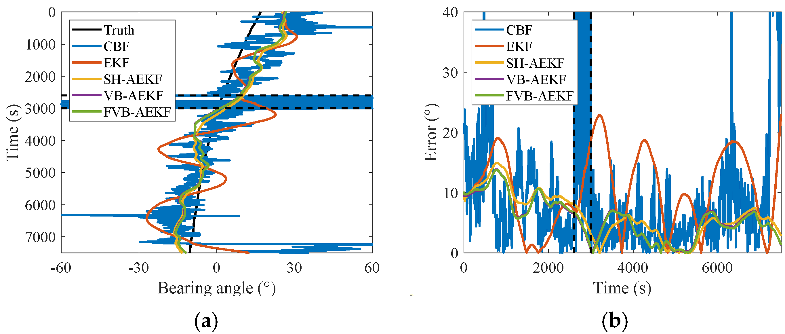
5.3.1. Sea Trial Data Processing for Single Underwater Target Bearing Tracking

The results of applying the CBF, EKF, SH-AEKF, VB-AEKF, and FVB-AEKF to process acoustic experimental data from the South China Sea in July 2021 are presented. The target was a ship emitting continuous acoustic signals while in motion, and the signals were received by a uniform circular array mounted on a moored buoy system. Since the experimental data had a relatively high signal-to-noise ratio (SNR) and small variations in measurement noise power, a segment of high-power noise was added to the original measurement data between 2600 s and 3000 s to test the robustness of the underwater target bearing tracking methods under uncertain measurement noise. The results are shown in Figure 2a,b and

Table 2. Average bearing estimation error (ABEE) of the CBF, EKF, SH-AEKF, VB-AEKF, and FVB-AEKF.

Method	CBF	EKF	SH-AEKF	VB-AEKF	FVB-AEKF
ABEE/(°)	19.9	12.2	7.3	6.5	6.5

. The black dashed lines in Figure 2a,b indicate the start and end times of the added noise. In Figure 2a, two dashed lines can be seen. The upper dashed line marks the start of the noise addition at 2600 s, while the lower one indicates the end at 3000 s. The figure demonstrates that during this period, the CBF estimation results show significant oscillations, indicating divergence. Similarly, in Figure 2b, the left dashed line indicates the start of the noise addition, and the right one marks its end. The region between the dashed lines illustrates the error data after noise was added. Due to the significant oscillations in the CBF estimates during this interval, the errors at each time step show considerable fluctuations, resulting in a distinct blue band in the figure.

Figure 2a,b illustrate that all the trajectories derived from raw experimental data fluctuate around the true trajectory due to underwater environmental noise. Figure 2a,b and Table 2 demonstrate that the VB-AEKF and FVB-AEKF offer the most accurate tracking among all the methods tested. The reason is that the VB-AEKF and FVB-AEKF not only use the kinematic model of the underwater target to predict its bearing angle but also accurately estimate the MNCM (model noise covariance matrix). The SH-AEKF shows lower tracking precision than the VB-AEKF and FVB-AEKF, as the VB iteration process provides a more accurate MNCM than the Sage–Husa algorithm. Trajectories obtained via the EKF exhibit greater fluctuations compared to those from the SH-AEKF, VB-AEKF, and FVB-AEKF due to the mismatch between the assumed stationary MNCM and the actual non-stationary MNCM. The CBF-based DOA estimation leads to the largest trajectory errors because it disregards the kinematic information of the underwater target.

Trajectories derived from the noise-added data in Figure 2a,b confirm similar conclusions as those mentioned above. Furthermore, even after adding noise, the VB-AEKF and FVB-AEKF still provide robust tracking, while the performance of the EKF- and CBF-based DOA estimations significantly deteriorates. The performance of the SH-AEKF is also slightly affected by noise, though it remains less precise than the VB-AEKF and FVB-AEKF. The ABEE derived from the noise-added data presented in Table 2 once again highlights the superior precision of the VB-AEKF and FVB-AEKF.

The runtime per time step for DOA estimation based on the CBF, including the methods of the EKF, VB-AEKF, and FVB-AEKF, is shown in

Table 3. Runtime per time step for the CBF, EKF, SH-AEKF, VB-AEKF, and FVB-AEKF.

Date	Runing Time/(ms)
	CBF	EKF	SH-AEKF	VB-AEKF	FVB-AEKF
Raw data	1.12	0.11	0.13	0.70	0.34
Data with noise	1.08	0.11	0.14	0.75	0.35

. In both the processing of the raw data and data with added noise, the runtime of the FVB-EKF is half that of the VB-AEKF. This further demonstrates that the FVB-EKF offers greater computational efficiency than the VB-EKF, with negligible performance loss when substituting the FVB-EKF for the VB-AEKF. The EKF and SH-AEKF require less time than the FVB-EKF but yield DOA trajectories with larger errors. Consequently, the FVB-AEKF demonstrates advantages in both robustness and accuracy.

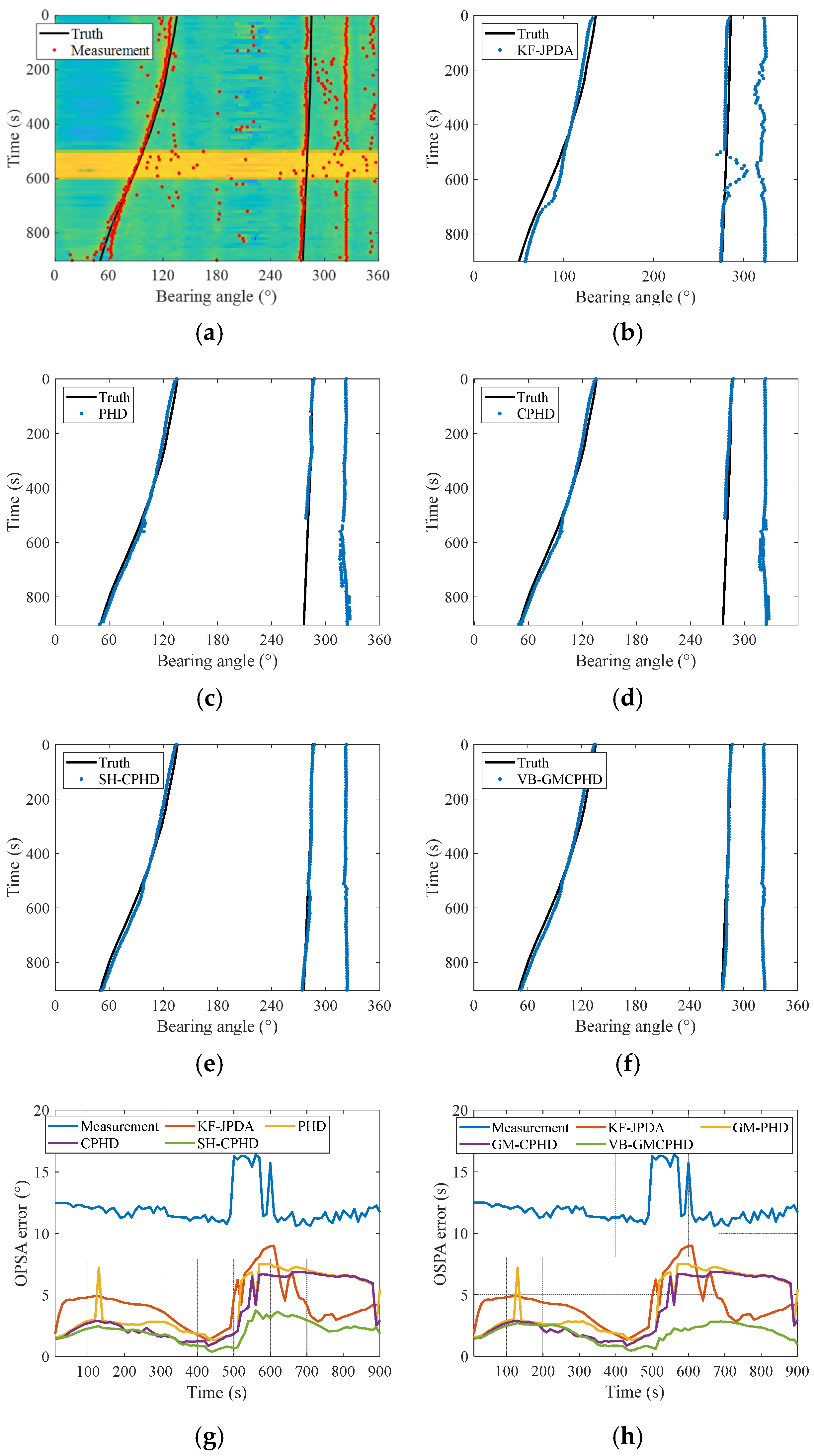
5.3.2. Processing of Experimental Data from Underwater Multi-Target Bearing Tracking Sea Trial

The following presents the results of applying various filtering methods—MVDR, KF-JPDA, PHD filter, CPHD filter, SH-CPHD filter, and VB-CPHD filter—to process data from the publicly available SWellEx96 dataset, focusing on the S59 event recorded by the northern horizontal line array. This experiment aims to track the bearing angle of three simultaneous targets. The original experimental data had a high signal-to-noise ratio (SNR) and minimal variation in the measurement noise power. To evaluate the robustness of underwater target bearing angle tracking methods under uncertain measurement noise conditions, we introduced a segment of high-power ocean environmental noise to increase the bearing angle measurement noise. The first step in the processing was using the MVDR method to estimate the target bearing angles every 10 s. These estimates included missed detections and false alarms. Figure 3a shows the bearing angle time history as a 3D color map in the background, while the target bearing angle measurements are indicated by red dots in the same figure. The bearing angle tracking results, based on these measurements, are illustrated in Figure 3b–f. The tracking performance, represented by the optimal sub-pattern assignment (OSPA) error, is depicted in Figure 3g,h. The average OSPA error and average runtime per tracking step are summarized in

Table 4. Average OSPA error and average runtime per tracking step for the KF-JPDA, PHD filter, CPHD filter, and SH-CPHD filter when processing experimental data with added noise.

	KF-JPDA	PHD	CPHD	SH-CPHD	VB-CPHD
Average OSPA Error (°)	4.26	4.22	3.71	2.06	1.97
Average Running Time (ms)	4.25	0.72	0.86	0.90	1.79

.

From Figure 3a, it can be observed that, due to the impact of marine environmental noise, the deviation of the bearing angle measurements from the true value is larger between 500 s and 600 s, resulting in increased false alarms and missed detections. From Figure 3b–h, the OSPA error of the bearing angle measurements significantly increases between 500 s and 600 s under noise influence. When the measurement noise variance is stable from 0 to 500 s, the KF-JPDA, PHD filter, and CPHD filter all achieve stable tracking of the three targets’ bearing angle. However, when the measurement noise variance increases between 500 s and 600 s, the discrepancy between the assumed constant noise variance and the increased true value in the KF-JPDA, PHD filter, and CPHD filter leads to inaccurate calculation of the Kalman filter gain. Consequently, tracking deviations or even track losses occur, leading to increased OSPA errors. In contrast, the OSPA error of the SH-CPHD filter’s robust multi-target bearing angle tracking method is significantly smaller than that of the other three tracking methods. This is because the SH-CPHD filter can estimate the measurement noise variance in real time during tracking, which makes the calculated Kalman filter gain more accurate. Therefore, the increase in noise variance has almost no effect on its tracking results, eliminating the impact of uncertain noise from the marine environment on the tracking performance and achieving robust underwater target bearing angle tracking. The VB-CPHD filter achieves the smallest OSPA error among all the methods for robust multi-target bearing angle tracking. This is because the VB-CPHD filter can estimate the measurement noise variance in real time based on a rigorous mathematical foundation and reasonable prior PDFs. Therefore, the Kalman filter gain calculated using these estimates is more accurate, rendering it nearly unaffected by changes in the measurement noise variance, thus ensuring robust underwater target bearing angle tracking under uncertain measurement noise. From Table 4, it can be seen that the VB-CPHD has a lower average OSPA error, but the improvement compared to the SH-CPHD is limited. Moreover, due to its reliance on a rigorous mathematical basis, the VB-CPHD significantly increases the computational load, with a computation time almost double that of the SH-CPHD. Therefore, the SH-CPHD and VB-CPHD are suitable for different application scenarios: the SH-CPHD is more appropriate in real-time scenarios with reliable historical measurements, while the VB-CPHD is better suited for situations requiring higher estimation accuracy.

5.4. Discussion

In single-target tracking scenarios, passive tracking—unlike active sonar or radar—does not produce clutter from stationary, silent objects. Even if clutter-generating objects are present, signal filtering based on the target’s frequency characteristics can further reduce the interference [140]. In such scenarios, without the complication of overlapping models, the array’s received signals can be treated as measurement signals, enhancing the accuracy of DOA estimates.

In multi-target tracking, passive tracking significantly reduces the clutter, but overlapping models in multi-target scenarios make effective separation challenging. The strategy begins with estimating the azimuth using DOA algorithms based on the target’s frequency characteristics, followed by filtering through multi-target tracking algorithms that incorporate kinematic features. Recent studies, such as those cited in reference [88], have shown that auxiliary features can significantly enhance the tracking accuracy by enabling passive sensors to quickly initiate and effectively track multiple non-cooperative targets. Compared to other methods, the featured approach offers advantages in terms of low energy consumption and minimal exposure across various settings, resulting in more accurate tracking. Another method outlined in reference [98] uses feature-assisted measurement partitioning algorithms to obtain efficient and accurate underwater measurements, improving the accuracy of tracking unknown targets.

6. Conclusions

In response to the urgent need for maritime environmental security, significant research has been conducted on passive underwater target bearing tracking technology, utilizing passive detection nodes as the hardware system. By integrating multi-source acoustic information, this approach offers benefits such as extensive coverage, prolonged observation periods, and real-time data fusion. It is an effective method for enhancing underwater target detection capabilities and represents a key direction in the development of acoustic target detection technologies in the marine environment. This paper provides a comprehensive review of the latest passive underwater target bearing tracking technologies. It details underwater target bearing estimation techniques and tracking technologies based on passive sonar platforms, focusing on methods, models, and robust adaptive tracking approaches. Additionally, it summarizes some results from sea trials. Although global research on underwater target bearing tracking has yielded preliminary results, more intensive and deeper investigations are still required. While this review may not be exhaustive, it aims to provide valuable references for interested readers.

References

1. Hou, X.; Qiao, G.; Zhou, J.; Yang, Y. Adaptive tracking algorithm for underwater maneuvering target based on vector dual quaternions. J. Harbin Eng. Univ. 2020, 41, 1444–1449, 1463. [Google Scholar]
2. Hou, X.; Yang, L.; Yang, Y.; Zhou, J.; Qiao, G. Bearing-only underwater uncooperative target tracking for non-Gaussian environment using fast particle filter. IET Radar Sonar Nav. 2022, 16, 501–514. [Google Scholar] [CrossRef]
3. Hou, X.; Zhou, J.; Yang, Y.; Yang, L.; Qiao, G. 3D underwater uncooperative target tracking for a time-varying non-Gaussian environment by distributed passive underwater buoys. Entropy 2021, 23, 902. [Google Scholar] [CrossRef] [PubMed]
4. Yang, L.; Yang, Y.; Wang, Y.; Zhuo, J. Direction-of-arrival estimation of a modified sparse asymptotic minimum variance approach. Acta Acust. 2016, 41, 465–476. [Google Scholar]
5. Yao, L.; Liu, X.; Cao, J.; Wang, S.; Zhang, D.; Wang, Y. Weighted beamspace direction-of-arrival estimation based on subarrays. Acta Acust. 2020, 45, 497–505. [Google Scholar]
6. Yang, Y.; Zhang, Y.; Yang, L. Wideband sparse spatial spectrum estimation using matrix filter with nulling in a strong interference environment. J. Acoust. Soc. Am. 2018, 143, 3891–3898. [Google Scholar] [CrossRef]
7. Yan, F.; Jin, M.; Qiao, X. Low-complexity DOA estimation based on compressed MUSIC and its performance analysis. IEEE Trans. Signal Process. 2013, 61, 1915–1930. [Google Scholar] [CrossRef]
8. Cao, R.; Liu, B.; Gao, F.; Zhang, X. A low-complex one-snapshot DOA estimation algorithm with massive ULA. IEEE Commun. Lett. 2017, 21, 1071–1074. [Google Scholar] [CrossRef]
9. Yan, H.; Fan, H.H. Signal-selective DOA tracking for wideband cyclostationary sources. IEEE Trans. Signal Process. 2007, 55, 2007–2015. [Google Scholar] [CrossRef]
10. Chen, W.; Zhang, W.; Wu, Y.; Chen, T.; Hu, Z. Joint algorithm based on interference suppression and Kalman filter for bearing-only weak target robust tracking. IEEE Access 2019, 7, 131653–131662. [Google Scholar] [CrossRef]
11. El-Hawary, F.; Jing, Y. Robust regression-based EKF for tracking underwater targets. IEEE J. Ocean. Eng. 1995, 20, 31–41. [Google Scholar] [CrossRef]
12. Zhang, B.; Hou, X.; Yang, Y. Robust underwater direction-of-arrival tracking with uncertain environmental disturbances using a uniform circular hydrophone array. J. Acoust. Soc. Am. 2022, 151, 4101–4113. [Google Scholar] [CrossRef] [PubMed]
13. Saucan, A.A.; Chonavel, T.; Sintes, C.; Le Caillec, J.M. Marked Poisson point process PHD filter for DOA tracking. In Proceedings of the 2015 23rd European Signal Processing Conference (EUSIPCO), Nice, France, 31 August–4 September 2015; pp. 2621–2625. [Google Scholar]
14. Saucan, A.A.; Chonavel, T.; Sintes, C.; Le Caillec, J.-M. Track before detect DOA tracking of extended targets with marked Poisson point processes. In Proceedings of the 2015 18th International Conference on Information Fusion (Fusion), Washington, DC, USA, 6–9 July 2015; pp. 754–760. [Google Scholar]
15. Saucan, A.A.; Chonavel, T.; Sintes, C.; Le Caillec, J.M. CPHD-DOA tracking of multiple extended sonar targets in impulsive environments. IEEE Trans. Signal Process. 2016, 64, 1147–1160. [Google Scholar] [CrossRef]
16. Masnadi-Shirazi, A.; Rao, B.D. A covariance-based superpositional CPHD filter for multisource DOA tracking. IEEE Trans. Signal Process. 2017, 66, 309–323. [Google Scholar] [CrossRef]
17. Li, G.; Wei, P.; Li, Y.; Chen, Y. A labeled multi-Bernoulli filter for multisource DOA tracking. In Proceedings of the 2019 International Conference on Control, Automation and Information Sciences (ICCAIS), Chengdu, China, 23–26 October 2019; pp. 1–6. [Google Scholar]
18. Zhao, J.; Gui, R.; Dong, X. A new measurement association mapping strategy for DOA tracking. Digit. Signal Process. 2021, 118, 103228. [Google Scholar] [CrossRef]
19. Yardim, C.; Michalopoulou, Z.H.; Gerstoft, P. An overview of sequential Bayesian filtering in ocean acoustics. IEEE J. Ocean. Eng. 2011, 36, 71–89. [Google Scholar] [CrossRef]
20. Qin, Y.; Zhang, H.; Wang, S. Principles of Kalman Filtering and Integrated Navigation, 3rd ed.; Northwestern Polytechnical University Press: Xi’an, China, 2015; pp. 33–35. [Google Scholar]
21. Guo, X.; Ge, F.; Guo, L. Improved adaptive Kalman filtering and its application in acoustic maneuvering target tracking. Acta Acust. 2011, 36, 611–618. [Google Scholar]
22. Sun, X.; Li, R.; Hu, P. A tracking filter method of active sonar subject to unknown target maneuvering. Acta Acust. 2016, 41, 371–378. [Google Scholar]
23. Hu, Y.; Sun, J. Study of underwater passive motion target analysis (TMA) in revised extended Kalman filter. Acta Acust. 2002, 27, 449–454. [Google Scholar]
24. Koteswara Rao, S.; Raja Rajeswari, K.; Lingamurty, K.S. Unscented Kalman filter with application to bearings-only target tracking. IETE J. Res. 2009, 55, 63–67. [Google Scholar]
25. Wang, P.; Liu, Y. Underwater target tracking algorithm based on improved adaptive IMM-UKF. J. Electron. Inf. Technol. 2022, 44, 1999–2005. [Google Scholar]
26. Leong, P.H.; Arulampalam, S.; Lamahewa, T.A.; Abhayapala, T.D. A Gaussian-sum based cubature Kalman filter for bearings-only tracking. IEEE T. Aero. Elec. Sys. 2013, 49, 1161–1176. [Google Scholar] [CrossRef]
27. Shi, G.; Yan, S.; Hao, C.; Hou, C.; Liu, Y. Target tracking algorithm for underwater ranges-only long baseline system with incomplete measurements. Acta Acust. 2019, 44, 480–490. [Google Scholar]
28. Orton, M.; Fitzgerald, W. A Bayesian approach to tracking multiple targets using sensor arrays and particle filters. IEEE Trans. Signal Process. 2002, 50, 216–223. [Google Scholar] [CrossRef]
29. Jin, S.; Li, Y.; Huang, H. A unified method for underwater multi-target bearing detection and tracking. Acta Acust. 2019, 44, 503–512. [Google Scholar]
30. Qiu, W.; Li, L.; Lei, P.; Wang, Z. Multiple targets tracking by using probability data association and cubature Kalman filter. In Proceedings of the 2018 10th International Conference on Wireless Communications and Signal Processing (WCSP), Hangzhou, China, 18–20 October 2018; pp. 1–5. [Google Scholar]
31. Li, X.; Willett, P.; Baum, M.; Baum, M.; Li, Y. PMHT approach for underwater bearing-only multisensory-multitarget tracking in clutter. IEEE J. Ocean. Eng. 2016, 41, 831–839. [Google Scholar] [CrossRef]
32. Xie, Z.; Jiang, C.; Wu, J.; Fang, Z.; Li, J. Method of multi-platform cooperative localization and tracking for underwater targets. Acta Acust. 2021, 46, 1028–1038. [Google Scholar]
33. Li, X.; Li, Y.; Lu, X.; Zhao, C.; Yu, J. Underwater bearing-only multitarget tracking in dense clutter environment based on PMHT. J. Northwestern Polytech. Univ. 2020, 38, 359–365. [Google Scholar] [CrossRef]
34. Yang, F.; Wang, Y.-Q.; Liang, Y.; Pan, Q. A survey of PHD filter based multi-target tracking. Acta Autom. Sin. 2013, 39, 1944–1956. [Google Scholar] [CrossRef]
35. Wang, X.; Han, C.; Lian, F. Research and latest developments on target tracking methods based on random finite sets. J. Eng. Math. 2012, 29, 567–578. [Google Scholar]
36. Mahler, R.P.S. Multitarget Bayes filtering via first-order multitarget moments. IEEE Trans. Aerosp. Electron. Syst. 2003, 39, 1152–1178. [Google Scholar] [CrossRef]
37. Vo, B.N.; Singh, S.; Doucet, A. Sequential Monte Carlo methods for multitarget filtering with random finite sets. IEEE Trans. Aerosp. Electron. Syst. 2005, 41, 1224–1245. [Google Scholar]
38. Clark, D.E.; Panta, K.; Vo, B.N. The GM-PHD filter multiple target tracker. In Proceedings of the 2006 9th International Conference on Information Fusion, Florence, Italy, 10–13 July 2006; pp. 1–8. [Google Scholar]
39. Mahler, R. A theory of PHD filters of higher order in target number. Proc. SPIE 2006, 6235, 193–204. [Google Scholar]
40. Mahler, R. PHD filters of higher order in target number. IEEE Trans. Aerosp. Electron. Syst. 2007, 43, 1523–1543. [Google Scholar] [CrossRef]
41. Yang, Y. Research on Sonar Beamforming and High-Resolution Direction Estimation Technology in Beam Domain. Ph.D. Thesis, Northwestern Polytechnical University, Xi’an, China, 2002. [Google Scholar]
42. Lee, J.H.; Park, Y.; Gerstoft, P. Compressive frequency-difference direction-of-arrival estimation. J. Acoust. Soc. Am. 2023, 154, 141–151. [Google Scholar] [CrossRef] [PubMed]
43. Cong, J.; Wang, X.; Huang, M.; Wan, L. Robust DOA estimation method for MIMO radar via deep neural networks. IEEE Sens. J. 2020, 21, 7498–7507. [Google Scholar] [CrossRef]
44. Cheng, Z.; Liao, B. QoS-aware hybrid beamforming and DOA estimation in multi-carrier dual-function radar-communication systems. IEEE J. Sel. Areas Commun. 2022, 40, 1890–1905. [Google Scholar] [CrossRef]
45. Yu, Y.; Mei, J.; Zhai, C.; Hui, J.; Hui, J. Sea trial researches on the measurements of passive source space distribution imaging and positioning. Acta Acust. 2009, 34, 103–109. [Google Scholar]
46. Yang, Y.; Yang, L.; Tang, J.; Feng, J. Sonar System Beamforming and Accurate Target Direction Estimation; Harbin Engineering University Press: Harbin, China, 2018. [Google Scholar]
47. Douglass, A.S.; Song, H.C.; Dowling, D.R. Performance comparisons of frequency-difference and conventional beamforming. J. Acoust. Soc. Am. 2017, 142, 1663–1673. [Google Scholar] [CrossRef]
48. Schmidt, R. Multiple emitter location and signal parameter estimation. IEEE Trans. Antennas Propag. 1986, 34, 276–280. [Google Scholar] [CrossRef]
49. Roy, R.; Paulraj, A.; Kailath, T. ESPRIT--A subspace rotation approach to estimation of parameters of cisoids in noise. IEEE Trans. Acoust. Speech Signal Process. 1986, 34, 1340–1342. [Google Scholar] [CrossRef]
50. Roy, R.; Kailath, T. ESPRIT-estimation of signal parameters via rotational invariance techniques. IEEE Trans. Acoust. Speech Signal Process. 1989, 37, 984–995. [Google Scholar] [CrossRef]
51. Dogan, M.C.; Mendel, J.M. Applications of cumulants to array processing. I. aperture extension and array calibration. IEEE Trans. Signal Process. 1995, 43, 1200–1216. [Google Scholar] [CrossRef]
52. Chevalier, P.; Ferréol, A.; Albera, L. High-resolution direction finding from higher order statistics: The 2rmq-MUSIC algorithm. IEEE Trans. Signal Process. 2006, 54, 2986–2997. [Google Scholar] [CrossRef]
53. Gonen, E.; Mendel, J.M.; Dogan, M.C. Applications of cumulants to array processing. IV. Direction finding in coherent signals case. IEEE Trans. Signal Process. 1997, 45, 2265–2276. [Google Scholar] [CrossRef]
54. Zeng, W.J.; Li, X.L. High-resolution multiple wideband and nonstationary source localization with unknown number of sources. IEEE Trans. Signal Process. 2010, 58, 3125–3136. [Google Scholar] [CrossRef]
55. Bush, D.; Xiang, N. A model-based Bayesian framework for sound source enumeration and direction of arrival estimation using a coprime microphone array. J. Acoust. Soc. Am. 2018, 143, 3934–3945. [Google Scholar] [CrossRef]
56. Madadi, Z.; Anand, G.V.; Premkumar, A.B. Three-dimensional localization of multiple acoustic sources in shallow ocean with non-Gaussian noise. Digit. Signal Process. 2014, 32, 85–99. [Google Scholar] [CrossRef]
57. Padois, T.; Berry, A. Orthogonal matching pursuit applied to the deconvolution approach for the mapping of acoustic sources inverse problem. J. Acoust. Soc. Am. 2015, 138, 3678–3685. [Google Scholar] [CrossRef]
58. Chen, T.; Wu, H.; Liu, L. A joint Doppler frequency shift and DOA estimation algorithm based on sparse representations for collocated TDM-MIMO radar. J. Appl. Math. 2014, 2014, 1–9. [Google Scholar]
59. Markopoulos, P.P.; Tsagkarakis, N.; Pados, D.A.; Karystinos, G.N. Direction-of-arrival estimation by L1-norm principal components. In Proceedings of the 2016 IEEE International Symposium on Phased Array Systems and Technology (PAST), Waltham, MA, USA, 18–21 October 2016; IEEE: Piscataway, NJ, USA, 2016; pp. 1–6. [Google Scholar]
60. Zheng, J.; Kaveh, M. Sparse spatial spectral estimation: A covariance fitting algorithm, performance and regularization. IEEE Trans. Signal Process. 2013, 61, 2767–2777. [Google Scholar] [CrossRef]
61. Xenaki, A.; Gerstoft, P.; Mosegaard, K. Compressive beamforming. J. Acoust. Soc. Am. 2014, 136, 260–271. [Google Scholar] [CrossRef] [PubMed]
62. Stoica, P.; Babu, P.; Li, J. SPICE: A sparse covariance-based estimation method for array processing. IEEE Trans. Signal Process. 2010, 59, 629–638. [Google Scholar] [CrossRef]
63. Stoica, P.; Babu, P.; Li, J. New method of sparse parameter estimation in separable models and its use for spectral analysis of irregularly sampled data. IEEE Trans. Signal Process. 2010, 59, 35–47. [Google Scholar] [CrossRef]
64. Yang, Z.; Xie, L.; Zhang, C. A discretization-free sparse and parametric approach for linear array signal processing. IEEE Trans. Signal Process. 2014, 62, 4959–4973. [Google Scholar] [CrossRef]
65. Abeida, H.; Zhang, Q.; Li, J.; Merabtine, N. Iterative sparse asymptotic minimum variance based approaches for array processing. IEEE Trans. Signal Process. 2012, 61, 933–944. [Google Scholar] [CrossRef]
66. Kalman, R.E. A new approach to linear filtering and prediction problems. J. Basic Eng. 1960, 82, 35–46. [Google Scholar] [CrossRef]
67. Crassidis, J.L.; Junkins, J.L. Optimal Estimation of Dynamic Systems, 2nd ed.; Chapman & Hall/CRC: Boca Raton, FL, USA, 2015; Volume 51, p. 591. [Google Scholar]
68. Senne, K. Review of Stochastic Processes and Filtering Theory-Andrew H. Jazwinski. IEEE Trans. Autom. Control 1972, 17, 752–753. [Google Scholar] [CrossRef]
69. Schmidt, S.F. The Kalman filter-Its recognition and development for aerospace applications. J. Guid. Control Dyn. 2012, 4, 4–7. [Google Scholar] [CrossRef]
70. Liu, C.; Zhou, Z.; Fu, X. Attitude determination for MAVs using a Kalman filter. Tsinghua Sci. Technol. 2008, 13, 593–597. [Google Scholar] [CrossRef]
71. Murrell, J.W. Precision attitude determination for multimission spacecraft. In Proceedings of the AIAA, Palo Alto, CA, USA, 7 August–9 August 1978. [Google Scholar]
72. Lefferts, E.; Markley, F.; Shuster, M.D. Kalman filtering for spacecraft attitude estimation. J. Guid. Control Dyn. 1982, 5, 417–429. [Google Scholar] [CrossRef]
73. Crassidis, J.L.; Markley, F.L.; Cheng, Y. Survey of nonlinear attitude estimation methods. J. Guid. Control Dyn. 2007, 30, 12–28. [Google Scholar] [CrossRef]
74. Julier, S.J.; Uhlmann, J.K.; Durrantwhyte, H.F. A new approach for filtering nonlinear systems. In Proceedings of the Advances in Computing and Communications, Seattle, WA, USA, 21–23 June 1995; pp. 1628–1632. [Google Scholar]
75. Julier, S.J.; Uhlmann, J.K. New extension of the Kalman filter to nonlinear systems. In Signal Processing, Sensor Fusion, and Target Recognition VI; International Society for Optics and Photonics: Bellingham, WA, USA, 1997. [Google Scholar]
76. Julier, S.J.; Uhlmann, J.K.; Durrantwhyte, H.F. A new method for the nonlinear transformation of means and covariances in filters and estimators. IEEE Trans. Autom. Control 2000, 45, 477–482. [Google Scholar] [CrossRef]
77. Romanenko, A.; Castro, J.A.A.M. The unscented filter as an alternative to the EKF for nonlinear state estimation: A simulation case study. Comput. Chem. Eng. 2004, 28, 347–355. [Google Scholar] [CrossRef]
78. Doucet, A. An introduction to sequential Monte Carlo methods. Seq. Monte Carlo Methods Pract. 2001, 18, 3–14. [Google Scholar]
79. Metropolis, N.; Rosenbluth, A.W.; Rosenbluth, M.N.; Teller, A.H.; Teller, E. Equation of state calculations by fast computing machines. J. Chem. Phys. 1953, 21, 1087–1092. [Google Scholar] [CrossRef]
80. Hammersley, J.M.; Morton, K.W. Poor man’s Monte Carlo. J. R. Stat. Soc. Ser. B Methodol. 1954, 16, 23–38. [Google Scholar] [CrossRef]
81. Gordon, N.J.; Salmond, D.J.; Smith, A.F.M. Novel approach to nonlinear/non-Gaussian Bayesian state estimation. IEE Proc. F-Radar Signal Process. IET 1993, 140, 107–113. [Google Scholar] [CrossRef]
82. Pitt, M.K.; Shephard, N. Filtering via simulation: Auxiliary particle filters. J. Am. Stat. Assoc. 1999, 94, 590–599. [Google Scholar] [CrossRef]
83. Wang, H. Improved extend Kalman particle filter based on Markov chain Monte Carlo for nonlinear state estimation. In Proceedings of the 2012 2nd International Conference on Uncertainty Reasoning and Knowledge Engineering (URKE), Jakarta, Indonesia, 14–15 August 2012; IEEE: Piscataway, NJ, USA, 2012; pp. 281–285. [Google Scholar]
84. Bar-Shalom, Y.; Fortmann, T.E.; Cable, P.G. Tracking and Data Association. J. Acoust. Soc. Am. 1990, 87, 918–919. [Google Scholar] [CrossRef]
85. Blackman, S. Design and Analysis of Modern Tracking Systems; Artech House: New York, NY, USA, 1999. [Google Scholar]
86. Bar-Shalom, Y. Multi-Target Multi-Sensor Tracking: Principles and Techniques; YBS Publishing: Storrs, CT, USA, 1995. [Google Scholar]
87. Bar-Shalom, Y.; Tse, E. Tracking in a cluttered environment with probabilistic data association. Automatica 1975, 11, 451–460. [Google Scholar] [CrossRef]
88. Tian, Y.; Liu, M.; Zhang, S.; Zheng, R.; Fan, Z. Feature-Aided Passive Tracking of Noncooperative Multiple Targets Based on the Underwater Sensor Networks. IEEE Internet Things J. 2023, 10, 4579–4591. [Google Scholar] [CrossRef]
89. Baser, E.; Bilik, I. Modified unscented particle filter using variance reduction factor. In Proceedings of the Radar Conference, Arlington, VI, USA, 10–14 May 2010; IEEE: Piscataway, NJ, USA, 2010; pp. 893–898. [Google Scholar]
90. Chen, J.; Leung, H.; Lo, T.; Litva, J.; Blanchette, M. A modified probabilistic data association filter in a real clutter environment. IEEE Trans. Aerosp. Electron. Syst. 1996, 32, 300–313. [Google Scholar] [CrossRef]
91. Roecker, J.A. A class of near-optimal JPDA algorithms. IEEE Trans. Aerosp. Electron. Syst. 1994, 30, 504–510. [Google Scholar] [CrossRef]
92. Musicki, D.; Evans, R. Joint integrated probabilistic data association: JIPDA. IEEE Trans. Aerosp. Electron. Syst. 2004, 40, 1093–1099. [Google Scholar] [CrossRef]
93. Zhu, Z. Iterated joint probabilistic data association. In Proceedings of the CIE International Conference of Radar, Beijing, China, 8–10 October 1996; pp. 434–438. [Google Scholar]
94. Deb, S.; Yeddanapudi, M.; Pattipati, K.; Bar-Shalom, Y. A generalized S-D assignment algorithm for multisensor-multitarget state estimation. IEEE Trans. Aerosp. Electron. Syst. 1997, 33, 523–538. [Google Scholar]
95. Lin, L.; Bar-Shalom, Y.; Kirubarajan, T. New assignment-based data association for tracking move-stop-move targets. IEEE Trans. Aerosp. Electron. Syst. 2004, 40, 714–725. [Google Scholar] [CrossRef]
96. Reid, D.B. An algorithm for tracking multiple targets. IEEE Trans. Autom. Control 1979, 24, 843–854. [Google Scholar] [CrossRef]
97. Vo, B.T.; Vo, B.N.; Cantoni, A. Analytic implementations of the cardinalized probability hypothesis density filter. IEEE Trans. Signal Process. 2007, 55, 3553–3567. [Google Scholar] [CrossRef]
98. Tian, Y.; Liu, M.; Zhang, S.; Zheng, R.; Dong, S.; Liu, Z. Underwater Target Tracking Based on the Feature-Aided GM-PHD Method. IEEE Trans. Instrum. Meas. 2024, 73, 5500412. [Google Scholar] [CrossRef]
99. Zhou, T.; Wang, Y.; Zhang, L.; Chen, B.; Yu, X. Underwater Multitarget Tracking Method Based on Threshold Segmentation. IEEE J. Ocean. Eng. 2023, 48, 1255–1269. [Google Scholar] [CrossRef]
100. Mahler, R. Statistical Multisource-Multitarget Information Fusion; Artech House: Norwood, MA, USA, 2007. [Google Scholar]
101. Vo, B.T.; Vo, B.N.; Cantoni, A. The cardinality balanced multi-target multi-Bernoulli filter and its implementations. IEEE Trans. Signal Process. 2009, 57, 409–423. [Google Scholar]
102. Feng, L.; Chen, L.; Han, C.; Chen, H. Convergence analysis for the SMC-MeMBer and SMC-CBMeMBer filters. J. Appl. Math. 2012, 3, 701–708. [Google Scholar]
103. Bar-Shalom, Y.; Willett, P.K.; Tian, X. Tracking and Data Fusion; YBS Publishing: Storrs, CT, USA, 2011. [Google Scholar]
104. Erdinc, O.; Willett, P.; Bar-Shalom, Y. Probability hypothesis density filter for multitarget multisensor tracking. In Proceedings of the 8th International Conference on Information Fusion, Philadelphia, PA, USA, 27 June–1 July 2005; pp. 1–8. [Google Scholar]
105. Mählisch, M.; Schweiger, R.; Ritter, W.; Dietmayer, K. Multisensor vehicle tracking with the probability hypothesis density filter. In Proceedings of the 9th International Conference on Information Fusion, Florence, Italy, 10–13 July 2006; pp. 1–8. [Google Scholar]
106. Fränken, D.; Schmidt, M.; Ulmke, M. “Spooky action at a distanc” in the cardinalized probability hypothesis density filter. IEEE Trans. Aerosp. Electron. Syst. 2009, 45, 1657–1664. [Google Scholar] [CrossRef]
107. Reuter, S. Multi-object tracking using random finite sets. Diss. Universität Ulm 2014. [Google Scholar]
108. Vo, B.-T.; Vo, B.-N.; Hoseinnezhad, R.; Mahler, R. Robust multiBernoulli filtering. IEEE J. Sel. Top. Signal Process. 2013, 7, 399–409. [Google Scholar] [CrossRef]
109. Reuter, S.; Meissner, D.; Wilking, B.; Dietmayer, K. Cardinality balanced multi-target multi-Bernoulli filtering using adaptive birth distributions. In Proceedings of the 16th International Conference on Information Fusion, Istanbul, Turkey 9–12 July 2013; pp. 1608–1615. [Google Scholar]
110. Dunne, D.; Kirubarajan, T. Multiple model multi-Bernoulli filters for manoeuvering targets. IEEE Trans. Aerosp. Electron. Syst. 2013, 49, 2679–2692. [Google Scholar] [CrossRef]
111. Shen, X.; Song, Z.; Fan, H.; Hu, Q. A general cardinalized probability hypothesis density filter. EURASIP J. Adv. Signal Process. 2022, 2022, 94. [Google Scholar] [CrossRef]
112. García-Fernández, Á.F.; Svensson, L. Trajectory PHD and CPHD filters. IEEE Trans. Signal Process. 2019, 67, 5702–5714. [Google Scholar] [CrossRef]
113. Vo, B.T.; Vo, B.N. Labeled random finite sets and multi-object conjugate priors. IEEE Trans. Signal Process. 2013, 61, 3460–3475. [Google Scholar] [CrossRef]
114. Papi, F.; Vo, B.N.; Vo, B.T.; Fantacci, C.; Beard, M. Generalized labeled multi-Bernoulli approximation of multi-object densities. IEEE Trans. Signal Process. 2015, 63, 5487–5497. [Google Scholar] [CrossRef]
115. Dong, X.; Zhao, J.; Sun, M.; Zhang, X.; Wang, Y. A Modified δ-Generalized Labeled Multi-Bernoulli Filtering for Multi-Source DOA Tracking with Coprime Array. IEEE Trans. Wireless Commun. 2023, 22, 9424–9437. [Google Scholar] [CrossRef]
116. Cai, H.; Houssineau, J.; Jones, B.A.; Jah, M.; Zhang, J. Possibility Generalized Labeled Multi-Bernoulli Filter for Multitarget Tracking Under Epistemic Uncertainty. IEEE Trans. Aerosp. Electron. Syst. 2023, 59, 1312–1326. [Google Scholar]
117. Lee, J.Y.; Shim, C.; Van Nguyen, H.; Nguyen, T.T.D.; Choi, H.; Kim, Y. Label Space Partition Selection for Multi-Object Tracking Using Two-Layer Partitioning. In Proceedings of the 2023 12th International Conference on Control, Automation and Information Sciences (ICCAIS), Hanoi, Vietnam, 27–29 November 2023; IEEE: Piscataway, NJ, USA, 2023. [Google Scholar]
118. Do, C.-T.; Nguyen, T.T.D.; Moratuwage, D.; Shim, C.; Chung, Y.D. Multi-object tracking with an adaptive generalized labeled multi-Bernoulli filter. Signal Process. 2022, 196, 108532. [Google Scholar] [CrossRef]
119. Shim, C.; Vo, B.-T.; Vo, B.-N.; Ong, J.; Moratuwage, D. Linear complexity Gibbs sampling for generalized labeled multi-Bernoulli filtering. IEEE Trans. Signal Process. 2023, 71, 1981–1994. [Google Scholar] [CrossRef]
120. Reuter, S.; Vo, B.T.; Vo, B.N.; Dietmayer, K. The Labeled multi Bernoulli filter. IEEE Trans. Signal Process. 2014, 62, 3246–3260. [Google Scholar] [CrossRef]
121. Nguyen, H.V.; Nguyen, T.T.D.; Shim, C.; Anuar, M. The Smooth Trajectory Estimator for LMB Filters. In Proceedings of the 2023 12th International Conference on Control, Automation and Information Sciences (ICCAIS), Hanoi, Vietnam, 27–29 November 2023; pp. 115–120. [Google Scholar]
122. Li, G.; Battistelli, G.; Chisci, L.; Gao, L.; Wei, P. Distributed Joint Detection, Tracking, and Classification via Labeled Multi-Bernoulli Filtering. IEEE Trans. Cybernet. 2024, 54, 1429–1441. [Google Scholar]
123. Li, G.; Li, G.; He, Y. Distributed Multiple Resolvable Group Targets Tracking Based on Hypergraph Matching. IEEE Sens. J. 2023, 23, 9669–9676. [Google Scholar]
124. Uney, M.; Stinco, P.; Dreo, R.; Micheli, M.; De Magistris, G.; Tesei, A. Passive Sensor Fusion and Tracking in Underwater Surveillance with the GLMB model. In Proceedings of the 2022 25th International Conference on Information Fusion (FUSION), Linköping, Sweden, 4–7 July 2022; pp. 1–8. [Google Scholar]
125. Mohinder, S.G. Kalman Filtering: Theory and Practice Using MATLAB; Angus, P.A., Ed.; Wiley: Hoboken, NJ, USA, 2001; pp. 133–144. [Google Scholar]
126. Zhou, H.; Jing, Z.; Wang, P. Maneuvering Target Tracking; National Defense Industry Press: Beijing, China, 1991; pp. 12–13. [Google Scholar]
127. Singer, R.A. Estimating optimal tracking performance for manned maneuvering targets. IEEE Trans. Aerosp. Electron. Syst. 1970, AES-6, 473–483. [Google Scholar] [CrossRef]
128. Moose, R.L. An adaptive state estimation solution to the maneuvering target problem. IEEE Trans. Autom. Control 1975, 20, 359–362. [Google Scholar] [CrossRef]
129. Zhou, H. Statistical Model of “Current” Maneuvering Target and Adaptive Tracking Algorithm. Aeronaut. Astronaut. Sin. 1983, 4, 72–86. [Google Scholar]
130. Mehrotra, K.; Mahapatra, P.R. A jerk model for tracking highly maneuvering targets. IEEE Trans. Aerosp. Electron. Syst. 1997, 33, 1094–1105. [Google Scholar] [CrossRef]
131. Blom, H.A.P.; Bar-Shalom, Y. The interacting multiple model algorithm for systems with Markovian switching coefficients. IEEE Trans. Autom. Control 1988, 33, 780–783. [Google Scholar] [CrossRef]
132. Dang, J. Underwater Multi-Target Tracking Theory; Northwestern Polytechnical University Press: Xi’an, China, 2009; p. 38. [Google Scholar]
133. Xu, J.; Xu, M.; Zhou, X. The bearing only target tracking of UUV based on cubature Kalman filter with noise estimator. In Proceedings of the 2017 36th Chinese Control Conference, Dalian, China, 26–28 July 2017; pp. 5288–5293. [Google Scholar]
134. Wang, X.; Xu, M.X.; Wang, H.B.; Wu, Y. Combination of interacting multiple models with the particle filter for three-dimensional target tracking in underwater wireless sensor networks. Math. Probl. Eng. 2012, 2012, 1–16. [Google Scholar] [CrossRef]
135. Zhang, J.X.; Liu, M.Q.; Fan, Z. Classify motion model via SVM to track underwater maneuvering target. In Proceedings of the 2019 IEEE International Conference on Signal Processing Communications and Computing, Dalian, China, 20–22 September 2019; pp. 1–6. [Google Scholar]
136. He, C.F.; Wang, Y.Y.; Chen, C.L.; Guan, X.P. Target localization for a distributed SIMO sonar with an isogradient sound speed profile. IEEE Access 2018, 6, 29770–29783. [Google Scholar] [CrossRef]
137. Ramezani, H.; Jamali-Rad, H.; Leus, G. Target localization and tracking for an isogradient sound speed profile. IEEE Trans. Signal Process. 2013, 61, 1434–1446. [Google Scholar] [CrossRef]
138. Zhang, D. Research on Self-Organizing Target Tracking Algorithm Based on Underwater Wireless Sensor Networks. Ph.D. Thesis, Zhejiang University, Hangzhou, China, 2019. [Google Scholar]
139. Liao, B.; Zhang, Z.G.; Chan, S.C. DOA estimation and tracking of ULAs with mutual coupling. IEEE Trans. Aerosp. Electron. Syst. 2012, 48, 891–905. [Google Scholar] [CrossRef]
140. Gao, X.; Li, X.; Jason, F.; Dai, W. A sequential Bayesian algorithm for DOA tracking in time-varying environments. Chin. J. Electron. 2015, 24, 140–145. [Google Scholar] [CrossRef]
141. Kong, D.; Chun, J. A fast DOA tracking algorithm based on the extended Kalman filter. In Proceedings of the IEEE 2000 National Aerospace and Electronics Conference, Dayton, OH, USA, 10–12 October 2000; pp. 235–238. [Google Scholar]
142. Cevher, V.; McClellan, J.H. General direction-of-arrival tracking with acoustic nodes. IEEE Trans. Signal Process. 2004, 53, 1–12. [Google Scholar] [CrossRef]
143. Cevher, V.; Velmurugan, R.; McClellan, J.H. Acoustic multitarget tracking using direction-of-arrival batches. IEEE Trans. Signal Process. 2007, 55, 2810–2825. [Google Scholar] [CrossRef]
144. Nannuru, S.; Coates, M.; Mahler, R. Computationally-tractable approximate PHD and CPHD filters for superpositional sensors. IEEE J. Sel. Top. Signal Process. 2013, 7, 410–420. [Google Scholar] [CrossRef]
145. Gao, X.; You, D.; Katayama, S. Seam tracking monitoring based on adaptive Kalman filter embedded elman neural network during high-power fiber laser welding. IEEE Trans. Ind. Electron. 2012, 59, 4315–4325. [Google Scholar] [CrossRef]
146. Mehra, R. Approaches to adaptive filtering. IEEE Trans. Automat. Control 1972, 17, 693–698. [Google Scholar] [CrossRef]
147. Mohamed, H.; Schwarz, K.P. Adaptive Kalman filtering for INS/GPS. J. Geod. 1999, 73, 193–203. [Google Scholar] [CrossRef]
148. Karasalo, M.; Hu, X.M. An optimization approach to adaptive Kalman filtering. Automatica 2011, 47, 1785–1793. [Google Scholar] [CrossRef]
149. Li, X.R.; Bar-Shalom, Y. A recursive multiple model approach to noise identification. IEEE Trans. Aerosp. Electron. Syst. 1994, 30, 671–684. [Google Scholar] [CrossRef]
150. Sarkka, S.; Nummenmaa, A. Recursive noise adaptive Kalman filtering by variational Bayesian approximations. IEEE Trans. Automat. Control 2009, 54, 596–600. [Google Scholar] [CrossRef]
151. Hartikainen, S.S.J. Variational Bayesian adaptation of noise covariance in nonlinear Kalman filtering. arXiv 2013, arXiv:1302.0681. [Google Scholar]
152. Huang, D.; Leung, H.; Naser, E.S. Expectation maximization-based GPS/INS integration for land-vehicle navigation. IEEE Trans. Aerosp. Electron. Syst. 2007, 43, 1168–1177. [Google Scholar] [CrossRef]
153. Bavdekar, V.A.; Deshpande, A.P.; Patwardhan, S.C. Identification of process and measurement noise covariance for state and parameter estimation using extended Kalman filter. J. Process Control 2011, 21, 585–601. [Google Scholar] [CrossRef]
154. Ardeshiri, T.; Ozkan, E.; Orguner, U.; Gustafsson, F. Approximate Bayesian smoothing with unknown process and measurement noise covariances. IEEE Signal Process. Lett. 2015, 22, 2450–2454. [Google Scholar] [CrossRef]
155. Huang, Y.; Zhang, Y.; Xu, B.; Wu, Z.; Chambers, J.A. A new adaptive extended Kalman filter for cooperative localization. IEEE Trans. Aerosp. Electron. Syst. 2017, 54, 353–368. [Google Scholar] [CrossRef]
156. Huang, Y.; Zhang, Y.; Wu, Z.; Li, N.; Chambers, J. A novel adaptive Kalman filter with inaccurate process and measurement noise covariance matrices. IEEE Trans. Autom. Control 2017, 63, 594–601. [Google Scholar] [CrossRef]
157. Xu, G.; Huang, Y.; Gao, Z.; Zhang, Y. A computationally efficient variational adaptive Kalman filter for transfer alignment. IEEE Sens. J. 2020, 20, 13682–13693. [Google Scholar] [CrossRef]
158. Hou, X.; Qiao, Y.; Zhang, B.; Yang, Y. Robust underwater direction-of-arrival tracking based on variational Bayesian extended Kalman filter. JASA Express Lett. 2023, 3, 014801. [Google Scholar] [CrossRef] [PubMed]
159. Ye, Z.; Xiang, L.; Xu, X. DOA estimation with circular array via spatial averaging algorithm. IEEE Antenn. Wirel. Propag. Lett. 2007, 6, 74–76. [Google Scholar] [CrossRef]
160. Hao, Y.; Zou, N.; Qiu, L.; Li, C.; Wang, Y.; Liang, G. Spatial rotation-based direction-of-arrival estimation for uniform circular hydrophone array. Appl. Acoust. 2021, 178, 107945. [Google Scholar] [CrossRef]
161. Zhang, B.; Hou, X.; Yang, Y. A fast variational Bayesian adaptive extended Kalman filter for robust underwater direction-of-arrival tracking. IEEE Sens. J. 2023, 23, 14709–14720. [Google Scholar] [CrossRef]
162. Zhang, B.; Yang, Y.; Hou, X. Robust underwater multi-target direction-of-arrival tracking with uncertain measurement noise. Acta Acust. 2023, 48, 605–617. [Google Scholar]
163. Zhang, B.; Hou, X.; Yang, Y. Variational Bayesian cardinalized probability hypothesis density filter for robust underwater multi-target DOA tracking with uncertain measurement noise. Front. Phys. 2023, 11, 1142400. [Google Scholar]
Figure 1. Logical diagram of various parts of the article.
Remotesensing 16 04511 g001
Figure 2. Experimental results of DOA estimation based on the CBF, EKF, SH-AEKF, VB-AEKF, and FVB-AEKF. (a) Trajectories obtained using noise-added data, and (b) bearing estimation error (BEE) obtained using noise-added data.
Remotesensing 16 04511 g002
Figure 3. The target bearing measurements and the target bearing tracking results and OSPA error for the KF-JPDA, PHD filter, CPHD filter, and SH-CPHD filter when processing experimental data with added noise. (a) Target bearing measurements, (b) KF-JPDA target bearing tracking results, (c) PHD filter target bearing tracking results, (d) CPHD filter target bearing tracking results, (e) SH-CPHD filter target bearing tracking results, (g) VB-CPHD filter target bearing tracking results, (h) SH-CPHD OSPA error in target bearing tracking results, and (f) SH-CPHD OSPA error in target bearing tracking results.
Remotesensing 16 04511 g003