Abstract
Terrestrial laser scanning (TLS) provides highly detailed 3D information of forest environments but is limited to small spatial scales, as data collection is time consuming compared to other remote sensing techniques. Furthermore, TLS data collection is heavily dependent on wind conditions, as the movement of trees negatively impacts the acquired data. Hardware advancements resulting in faster data acquisition times have the potential to be valuable in upscaling efforts but might impact overall data quality. In this study, we investigated the impact of the pulse repetition rate (PRR), or pulse frequency, which is the number of laser pulses emitted per second by the scanner. Increasing the PRR reduces the scan time required for a single scan but decreases the power (amplitude) of the emitted laser pulses commensurately. This trade-off could potentially impact the quality of the acquired data. We used a RIEGL VZ400i laser scanner to test the impact of different PRR settings on the point cloud quality and derived tree structural metrics from individual tree point clouds (diameter, tree height, crown projected area) as well as quantitative structure models (total branch length, tree volume). We investigated this impact across five field plots of different forest complexity and canopy density for three different PRR settings (300, 600 and 1200 kHz). The scan time for a single scan was 180, 90 and 45 s for 300, 600 and 1200 kHz, respectively. Differences among the raw acquired scans from different PRR replicates were largely removed by several necessary data processing steps, notably the removal of uncertain points with a low reflectance attribute. We found strong agreement between the individual tree structural metrics derived from each of the PRR replicates, independent of the forest complexity. This was the case for both point cloud-based metrics and those derived from quantitative structural models (QSMs). The results demonstrate that the PRR in high-end TLS instruments can be increased for data collection with negligible impact on a selection of derived structural metrics that are commonly used in the context of aboveground biomass estimation.
1. Introduction
Aboveground biomass (AGB) is crucial in the context of global carbon budgets as well as ecosystem monitoring [1]. Therefore, the need to accurately and consistently estimate AGB on a global scale has driven the development of Earth Observation (EO) missions for this purpose. These and future EO missions could reduce uncertainties about global carbon stocks and fluxes, but they depend on accurate and independent ground-based estimates of AGB for both the calibration of the EO methods and the validation of the resulting products [2]. However, ground-based AGB estimates are difficult to measure via traditional forestry methods and require destructive sampling for the calibration of the allometric models, which is an impractical, time-consuming and expensive process. Moreover, these costs scale with tree size and, thus, larger trees are less often sampled in reference data [3].
Advancements in laser scanning hardware and processing algorithms have enabled the collection of three-dimensional in situ data for forest structures [4]. By combining terrestrial laser scanning (TLS) with quantitative structure models (QSMs), a type of geometric model that reconstructs trees by fitting cylinders to point cloud data, a non-destructive estimate of tree volume, can be made. These tree volume estimates can then be used to derive AGB estimates by multiplying tree volume by wood density. This method to derive AGB estimates from TLS data has been benchmarked against destructive measurements [5,6,7,8]. Most of these studies used leaf-on data and reported a small overestimation (5–10%) of TLS-derived AGB compared to the destructively sampled reference. However, Gonzalez de Tanago et al. [7] reported a small underestimation (−3.7%) for tropical trees across Peru, Guyana and Indonesia. In any case, the reported biases were smaller compared to the biases from allometric models, for which underestimations up to 36.6% have been reported [5]. Therefore, TLS has been identified as an important component of accurate calibration and validation data for EO-derived AGB [9].
Despite the advantages compared to destructive measurements, TLS is still a relatively time-consuming measurement technique, which requires multiple different positions to obtain sufficient viewpoints. The survey of a 1 ha plot can typically take several days [10], depending on terrain and forest complexity, as the scanner needs to be moved between positions manually by the operator. Furthermore, TLS data collection is also heavily weather-dependent, as both wind and rain can impact the data negatively. Rain can damage the TLS equipment, add noise to the data and impact leaf and branch angles in the tree, due to the added weight of the water. Wind, on the other hand, can have a major negative impact by causing a “ghosting effect” in the point clouds, due to moving branches, which can introduce errors in tree volume estimates. Therefore, planning a TLS fieldwork campaign can be challenging, and the duration of a campaign can fluctuate significantly, depending on the weather conditions.
Over the last decade, newer TLS instrument models on the market have included improved hardware and software that enable the user to collect and register data faster, reducing both total scanning and processing time. These advancements could provide major benefits and time gains for TLS campaigns in forest environments, but the performance assessments are often made against TLS core user (build environment) cases, so it is often uncertain how these settings might affect data quality in a forest context, with more complex structures and environmental influences. One potential way to increase scanning speed is by increasing the pulse repetition rate (PRR), which represents the number of laser pulses that are emitted each second by the scanning device. Increasing the PRR will reduce the time needed to emit the same amount of laser pulses (i.e., increase the scanning frequency) and, thus, decrease the required scan time for a given amount of laser pulses. This decrease in scan time is a major advantage during a TLS campaign, for the reasons outlined above. There is a direct time gain, which scales linearly with the PRR increase. If the PRR is doubled, the scan time is halved. In addition to the direct time gain, shorter scan times also improve the ability to capture the often limited time windows of low wind conditions or avoid gusts while scanning. This is invaluable in the field, especially in wind-prone regions.
However, there is a trade-off between the PRR and other scanning characteristics. In TLS systems that operate using a multi-facet rotating mirror, laser pulses are generated by a fixed laser beam that is emitted into a rotating mirror, which then scatters a range of pulses into the environment. Increasing the PRR can thus be achieved by increasing the rotation speed of the mirror [11]. However, since the power of the source laser beam remains constant, the amplitude of each individual emitted laser pulse will decrease when the PRR is increased. This means that the individual pulses carry less energy (i.e., reduced amplitude of the outgoing laser pulse) and the signal-to-noise ratio of the returning pulses will be lower. Consequently, it requires less energy loss for a laser pulse to fall below the detection threshold, which can affect the penetration capacity through foliage. This effect is inversely linear, meaning that doubling the PRR will halve the energy (amplitude) of the outgoing laser pulses (personal communication with RIEGL). Furthermore, the PRR also affects the distance over which pulses can be resolved unambiguously, referred to as the unambiguous range. Beyond this unambiguous range, so-called multiple-time-around echoes introduce uncertainty as to which return belongs to which emitted pulse. Such echoes occur when the time for a pulse to reach a target at a certain distance and return to the scanner becomes longer than the time in between two consecutive pulses. The shorter the time between each pulse, the shorter that distance becomes and, thus, the unambiguous range decreases as the PRR increases. In a forest environment, observed ranges are usually relatively low, as 99% of the data has been found to be collected within the first 31 m to 109 m from the scanner, depending on the complexity of the forest [12]. As long as the nominal unambiguous range of a TLS device at a certain PRR exceeds those observed ranges, the decrease of the unambiguous range should not be a limitation in forest applications. Finally, the increase in scanning frequency might affect the distribution of scanner specific point attributes, such as reflectance or deviation. These attributes are used to remove noise points in raw point clouds [13], so strong shifts in the distributions of these point attributes could, thus, result in the removal of points with different quality levels.
While the technical implications (specifications are provided by the manufacturer) of an increased PRR are relatively well known (minimum, maximum and unambiguous ranges, as well as return number), the impact on the resulting point clouds in vegetated environments and any product derived from them is not well understood. In this study, we investigated the impact of three different PRRs (300, 600 and 1200 kHz) on the point clouds of forests with different structural complexity. Although the impact of an increased PRR is theoretically minimal for a typical forest AGB configuration, we understood that the complex scene could result in secondary effects of the PRR on the distribution of the points and their attributes in a single scan. We looked at the level of individual tree point clouds and investigated the differences in the structural tree metrics derived from each PRR replicate. The results demonstrate the effect of the PRR on several tree structural metrics that are commonly used to derive biomass estimates, either directly or as an input for biomass allometries. The results will enable better-informed decisions in regards to scanning frequencies in future TLS campaigns, leading to more efficient use of critical resources to collect forest point cloud data.
2. Materials and Methods
2.1. Equipment
The results from this study are based on the data from a RIEGL VZ400i scanner (RIEGL Laser Measurement Systems GmbH, Horn, Austria) [11]. This is a time-of-flight scanner that sends out infrared (1550 nm) laser pulses, using a multi-facet rotating mirror. The field of view of the device is 100° along the zenith and 360° along the azimuth. The exit beam diameter is 7 mm and the beam divergence is 0.35 mrad. The scanner has four different PRR settings: 100 kHz, 300 kHz, 600 kHz and 1200 kHz, each impacting other scanner performance metrics (Table 1). In this study, only the latter three PRR settings were evaluated, as the scan duration at 100 kHz becomes prohibitively long, hindering the ability to ensure minimal wind effects. The specifications for the minimum, maximum and unambiguous ranges for the different PRRs are also reproduced in Table 1. For ∼0.2, typical of vegetation reflectance, the most limited maximum range for 1200 kHz exceeded the nominal ranges seen in previous studies [12], suggesting that for typical forest applications this technical limitation is not a limiting factor. The same scanner model and scanning settings were used for all data acquisition, in order to keep all conditions constant, except for the PRR, and to ensure data comparability.

Table 1.
Specifications per pulse repetition rate (PRR), as listed by the manufacturer of the RIEGL VZ400i (datasheet RIEGL VZ-400i).
2.2. Data Collection
The data were collected in four forest plots, each representing different forest compositions (Figure 1, Table 2). The temperate deciduous forest plot was scanned in both leaf-off and leaf-on conditions. At each site, a square plot was laid out, consisting of 16 different scan locations. These scan locations were spaced on a 10 × 10 m or 15 × 15 m grid, depending on the canopy density and forest structural complexity [10], covering an area of 30 × 30 m or 45 × 45 m, respectively. A 10 × 10 m grid was chosen for both the tropical and conifer plot, because more occluding elements, such as understory vegetation and dense canopies, were expected in these plots, whereas a 15 × 15 m grid was used in the temperate and Eucalyptus plots. A fixed angular sampling resolution of 0.04° was used.

Figure 1.
Overview of the different terrestrial laser scanning (TLS) sites, using pictures captured from the scanner. Left to right: BEoff, BEon, AUS, GAB, UK.

Table 2.
Overview of the different plots, their forest types and data collection details.
At each scan location, the scanner was securely mounted on a surveying tripod. Because the zenith angle range of the instrument was limited to between 30° and 130°, an additional scan was captured at each sampling location, with the instrument tilted at 90° to sample the full sphere. Firstly, three scans were taken in the upright position, keeping all scanner settings the same except for the pulse repetition rate (PRR) at 300 kHz, 600 kHz and 1200 kHz. After these three upright scans, the instrument was tilted 90°, and scans with PRR 300 kHz, 600 kHz and 1200 kHz were captured. This resulted in three versions of the plot scale data, one for each different PRR setting. From here on, these three versions will be referred to as PRR replicates.
At the fixed 0.04° angular resolution, the scan time for a single scan at a PRR of 300 kHz was 3 min. For the higher PRR settings, the scan duration decreased linearly, resulting in a scan time of 1 min 30 s and 45 s for 600 kHz and 1200 kHz, respectively.
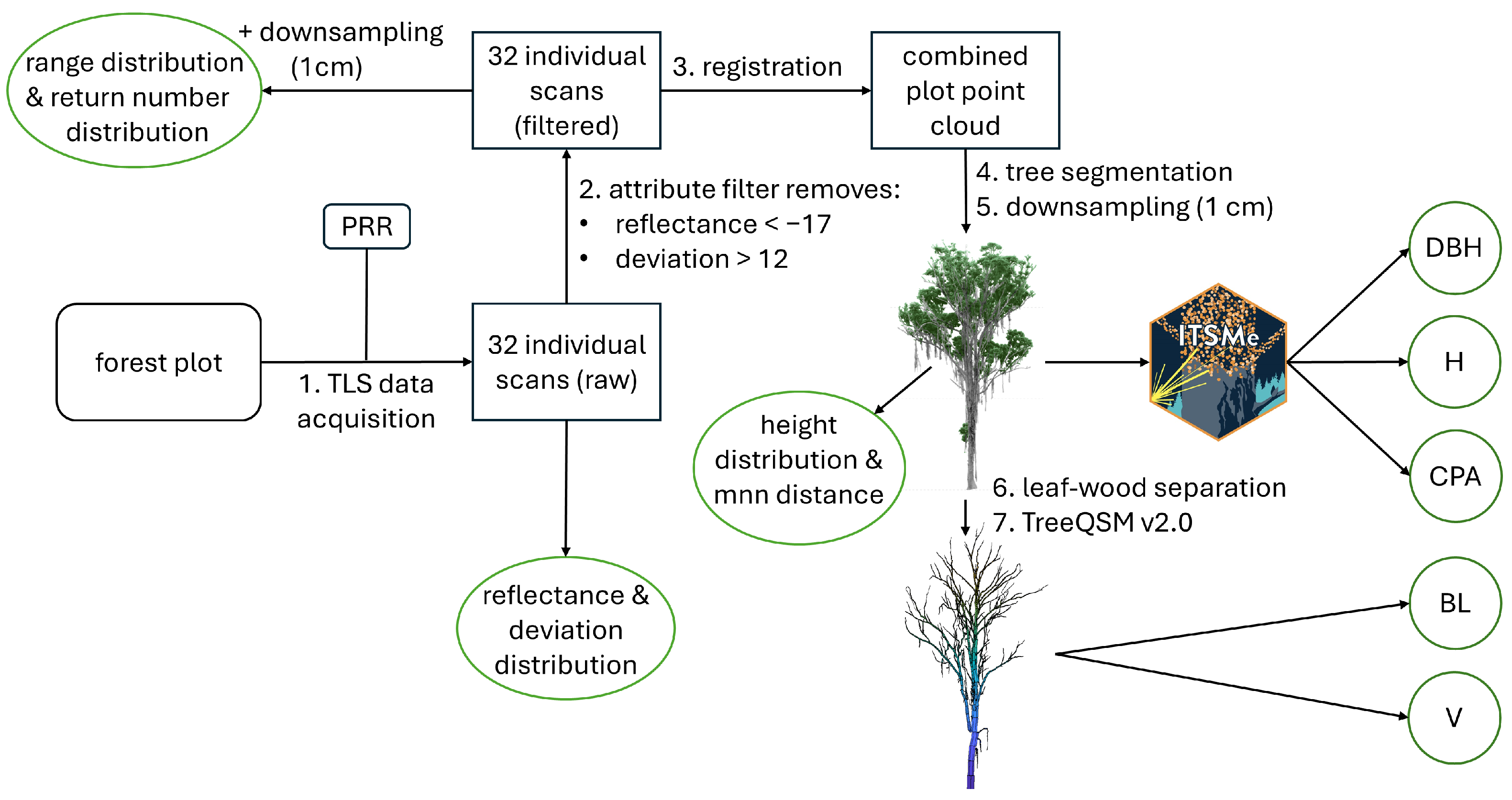
After the raw data were collected, an identical processing workflow was followed on every PRR replicate of every forest plot, to investigate possible impacts of the PRR on the data (Figure 2).
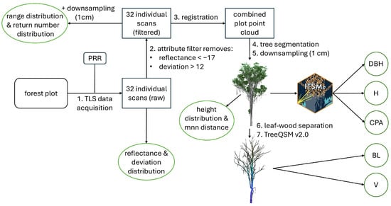
Figure 2.
Flowchart of the processing workflow that was followed to process the data from every PRR replicate (300, 600 and 1200 kHz) of each forest plot (BEoff, BEon, AUS, GAB, UK). Along the processing chain, the outputs that were compared among the different PRR replicates are indicated (green circles). On the level of individual scans, the differences in four point attribute distributions among the PRR replicates were investigated: reflectance, deviation, range and return number. The differences in the reflectance and deviation attributes were assessed on the raw collected scans, whereas the range and return number distributions were assessed for the data after a noise-filtering step (based on reflectance and deviation). After this, the individual scans were co-registered and individual tree point clouds were segmented from the resulting plot point clouds. The segmented point clouds were then used to investigate differences among the PRR replicates on the level of individual trees, looking at both the point distribution and sparsity along the tree height as well as the derived tree structural metrics. The extracted tree structural metrics were diameter at breast height (DBH), tree height (H), crown projected area (CPA), branch length (BL) and total tree volume (V).
2.3. Impact of PRR on Single Scans
Reflectance and pulse shape deviation were considered as two attributes of interest, to assess the impact of the PRR on the distribution of the point attributes in the raw data from a single scan, as these were used to filter noise out of the raw data [13]. The reflectance attribute depicts the apparent reflection of the target hit and can be used to filter noise points with low backscattered energy. The pulse shape deviation attribute reflects the change in the pulse shape of a return and can be used to remove points that might originate from merged return pulses from several intersected surfaces [6]. Pulse shape deviation is a unitless attribute. The same scan location was selected in every plot, and the distributions of both attributes were calculated for every scan that was taken on that location (six scans in total, one for every PRR in both up and tilt positions). The analyses were done in R v4.3.0 [14], using the data.table v1.14.8 package [15].
After this initial step, the single-scan point clouds were filtered by reflectance and deviation. Because no major differences between the PRR replicates were found in the overall trends of the distributions of both reflectance and deviation, similar cut-off thresholds as those previously used in the literature were selected. All points with reflectance lower than −17 dB or deviation higher than 12 were removed [13]. We elected to remove these points before further analysis, because we were most interested in the effect of the PRR on points that would be kept in practical applications. Two other point attributes were then investigated: the range distribution of the remaining points from the scanner and the number of returns. The range distribution was plotted for each PRR replicate.
Next, the point clouds were downsampled in CloudCompare v2.12.4. [16], using the spatial subsampling function with the minimal space between points set to 1 cm. This function divides the point cloud in an octree and picks a point in every cube, so that every point is minimally 1 cm apart. Downsampling is a common step in the processing of point cloud data, as it significantly reduces the amount of redundant points, which facilitates further analysis, and it leads to more uniform point densities across the cloud [17,18]. After downsampling, both the range distribution and number of returns were investigated once more.
2.4. Impact of PRR on Individual Tree Point Clouds
Next, the impact of different PRR settings at individual-tree level was investigated. The respective, filtered scans from every plot were co-registered in the scanner manufacturer’s RiSCAN PRO v2.18 software, to create a combined point cloud of each plot in every PRR replicate. A selection of the individual trees in each of the PRR replicates was then manually segmented for every plot. In total, 80 trees were selected for segmenting from across all the forest plots. The trees were semi-randomly selected, aiming to represent the range of tree sizes in the plot. Manual segmentation was chosen over (semi-)automated algorithms [19,20], to ensure the highest segmentation quality and avoid apparent differences due to segmentation errors. The resulting individual tree point clouds were then downsampled, using the spatial subsampling CloudCompare command at 1 cm, identical to the single scans in Section 2.3.
2.4.1. Point Distribution and Occlusion in Individual Trees
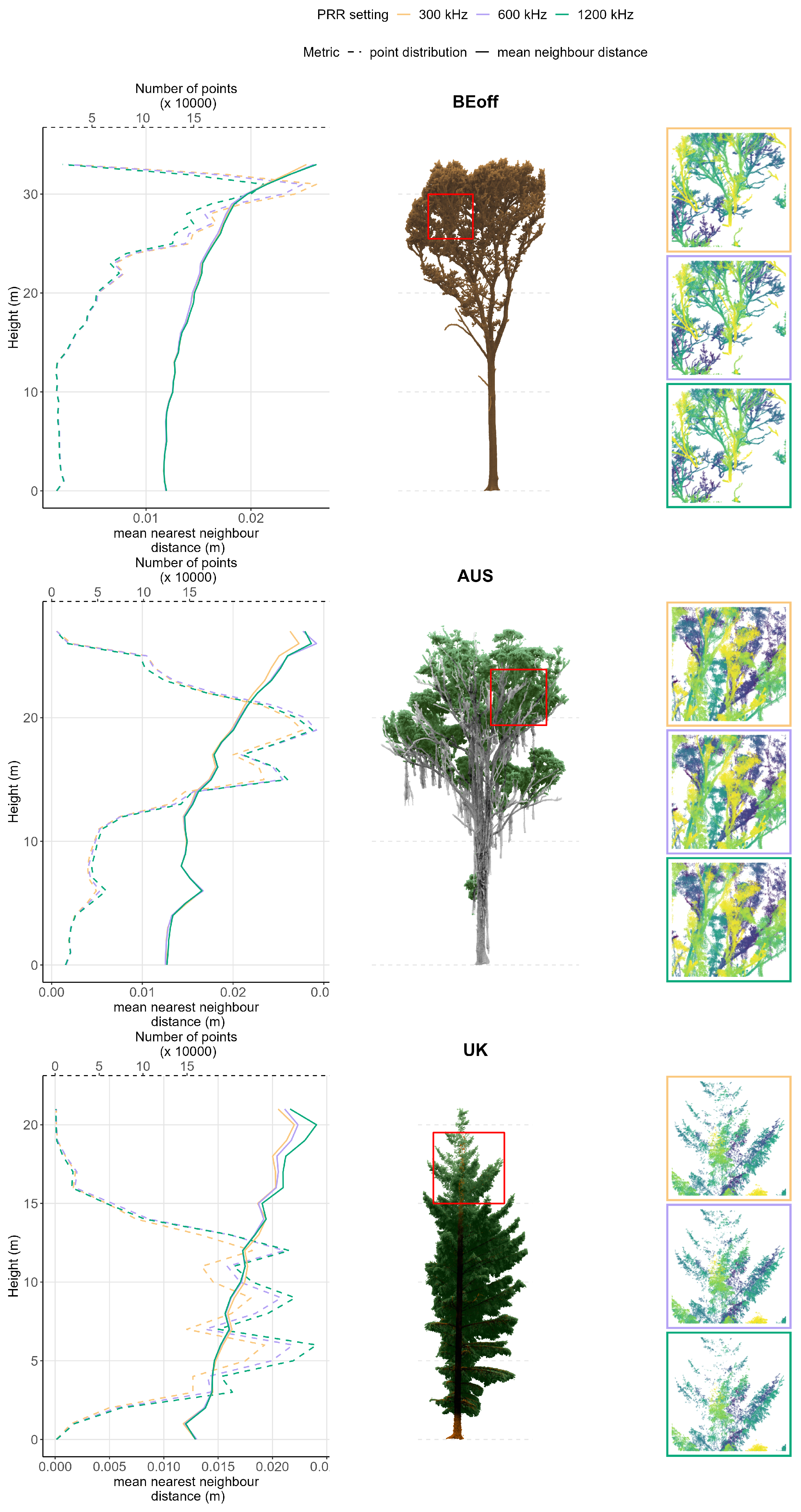
The impact of the PRR on the level of occlusion and overall point distribution in the individual tree point clouds was assessed both visually and quantitatively. A visual comparison among the PRR replicates from a selection of the largest trees in each plot was made first, to check for noticeable changes in canopy occlusion. After this, the differences in point density and/or occlusion levels among the different PRR replicates was also quantitatively assessed, using two metrics across the tree height. The first metric was simply the total number of points in each 1 m height bin. The second metric was the mean nearest neighbour distance and was calculated by averaging the mean distance to the four nearest neighbours for every point in a given height bin, similar to the metric used by Wilkes et al. [10]. Both metrics were calculated in R, using the lidR v4.0.4 package [21,22]. The mean nearest neighbour distance was calculated using the point_metrics function in this package.
2.4.2. Point Cloud Metrics
Three structural metrics were derived directly from the tree point clouds and evaluated among the different PRR replicates: diameter at breast height (DBH), tree height (H) and crown projected area (CPA). These three metrics were calculated using the ITSMe v1.0.1 R package [23]. The level of agreement between the metric values of the different PRR replicates was then assessed, using the concordance correlation coefficient (CCC). The CCC demonstrates how many data from two methods deviate from the line of perfect concordance (the 45° line on a square scatterplot) and ranges between 1 (perfect concordance) and −1 (perfect discordance) [24]. The CCC was calculated using the CCC function in the R package DescTools v0.99.50 [25].
2.4.3. Quantitative Structural Models
Finally, quantitative structural models (QSMs) were constructed for each PRR replicate of all the segmented trees. A leaf–wood separation was first needed, to isolate the woody elements within the tree point cloud (all plots except BEoff), which has been reported to improve QSM-based volume estimates [26]. This was done using a graph-based leaf–wood separation that purely used the xyz information of the tree point clouds [27]. Finally, the tree point clouds were downsampled further to 2.6 cm, to match with the TreeQSM workflows that had been benchmarked [18]. QSMs were then constructed, using a TreeQSM v2.0 workflow [5] for every PRR replicate of each segmented tree in every plot. This workflow built upon [28] and fitted cylinders to the segmented points clouds. A parameter optimization was needed to construct representative QSMs, and this optimization was conducted individually for every tree and every PRR replicate. Two metrics were then derived from the QSMs: the branch length (BL) and the total tree volume (V). Due to high occlusion in the UK conifer plot, large sections of the tree stems were occluded in the canopy of this plot, and it was elected not to construct QSMs for the trees in this plot.
3. Results
3.1. Impact of PRR on Single Scans
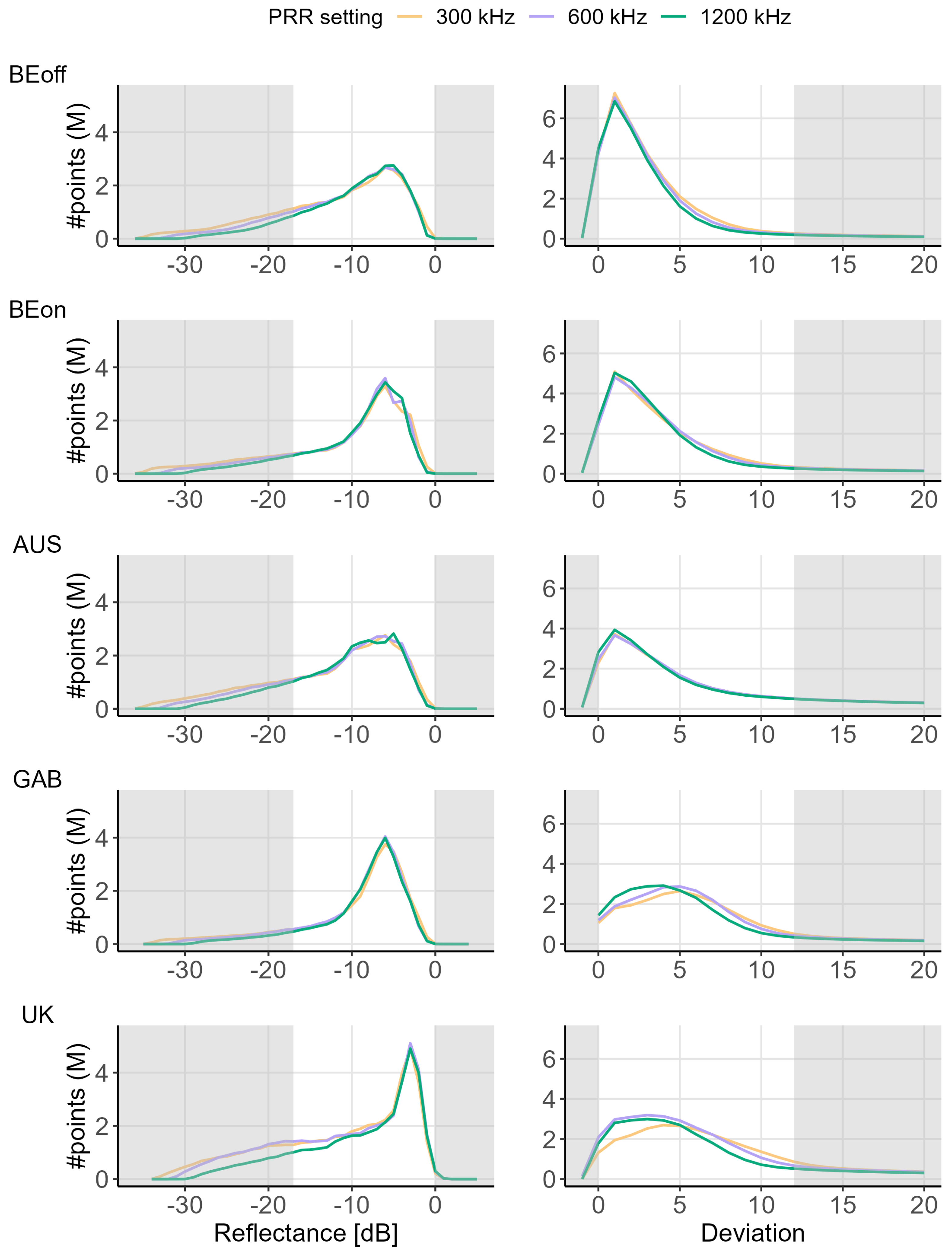
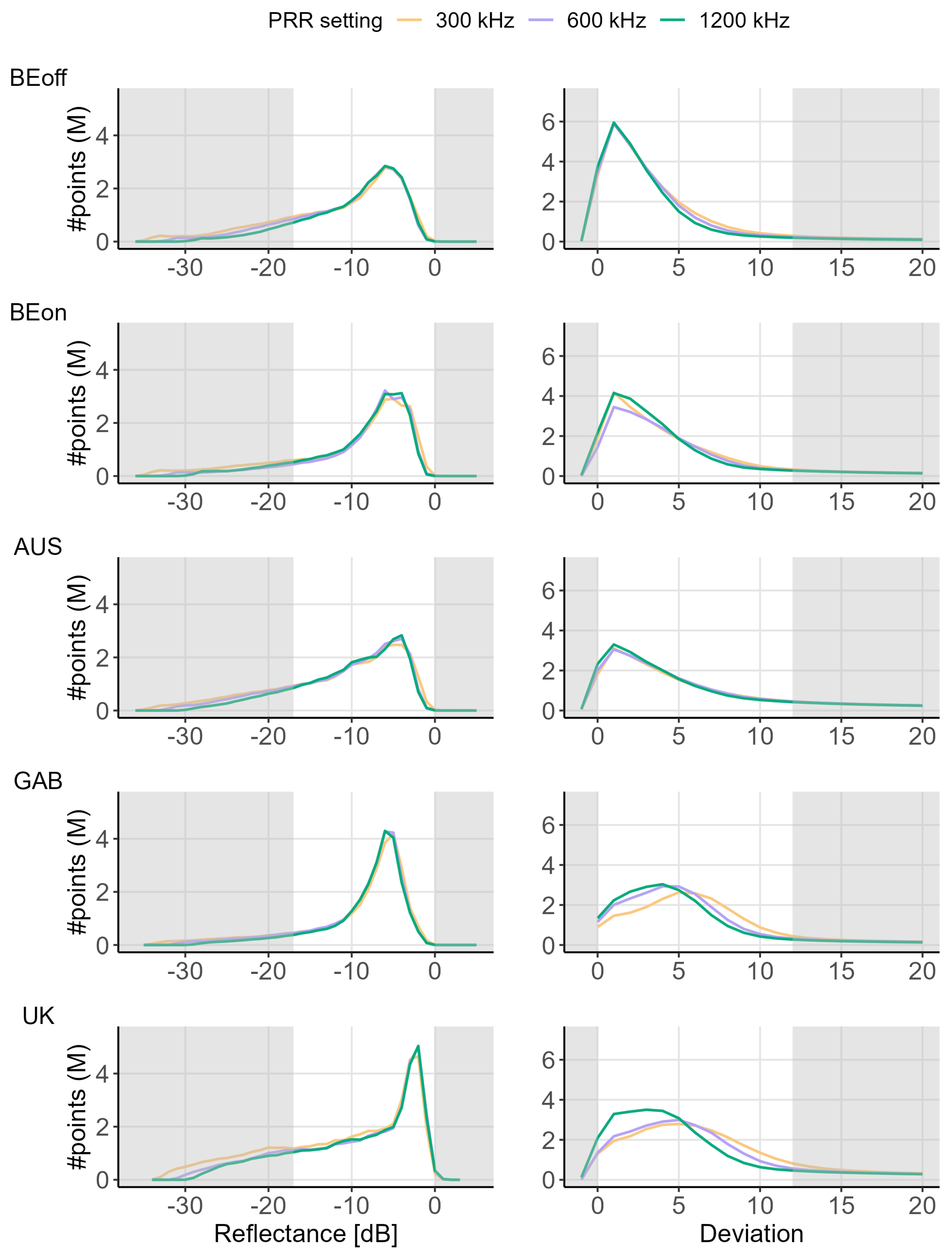
The overall trends in the distribution of reflectance and deviation in the raw data from a scan were found to be largely the same across the PRR replicates, although some small differences were still observed (Figure 3). For the GAB and UK plots, we observed sharper reflectance peaks but wider deviation peaks compared to the other plots. In the plots with wider deviation peaks, there were also small shifts in the locations of the peaks, with peaks from the higher PRR replicates located at slightly lower deviation values. Similar distributions were found for the tilt scans from the same locations (Appendix A Figure A1).
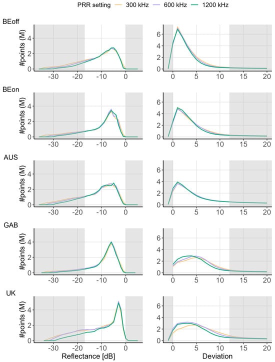
Figure 3.
Overview of the reflectance and deviation distributions in the raw data collected from the same single upright scan position with different pulse repetition rate (PRR) settings (top to bottom: BEoff, BEon, AUS, GAB, UK). The distributions show the number of points (millions) across the reflectance and distribution ranges. The grey bands indicate the areas from the distributions that were filtered out in the processing steps to remove high uncertainty points.
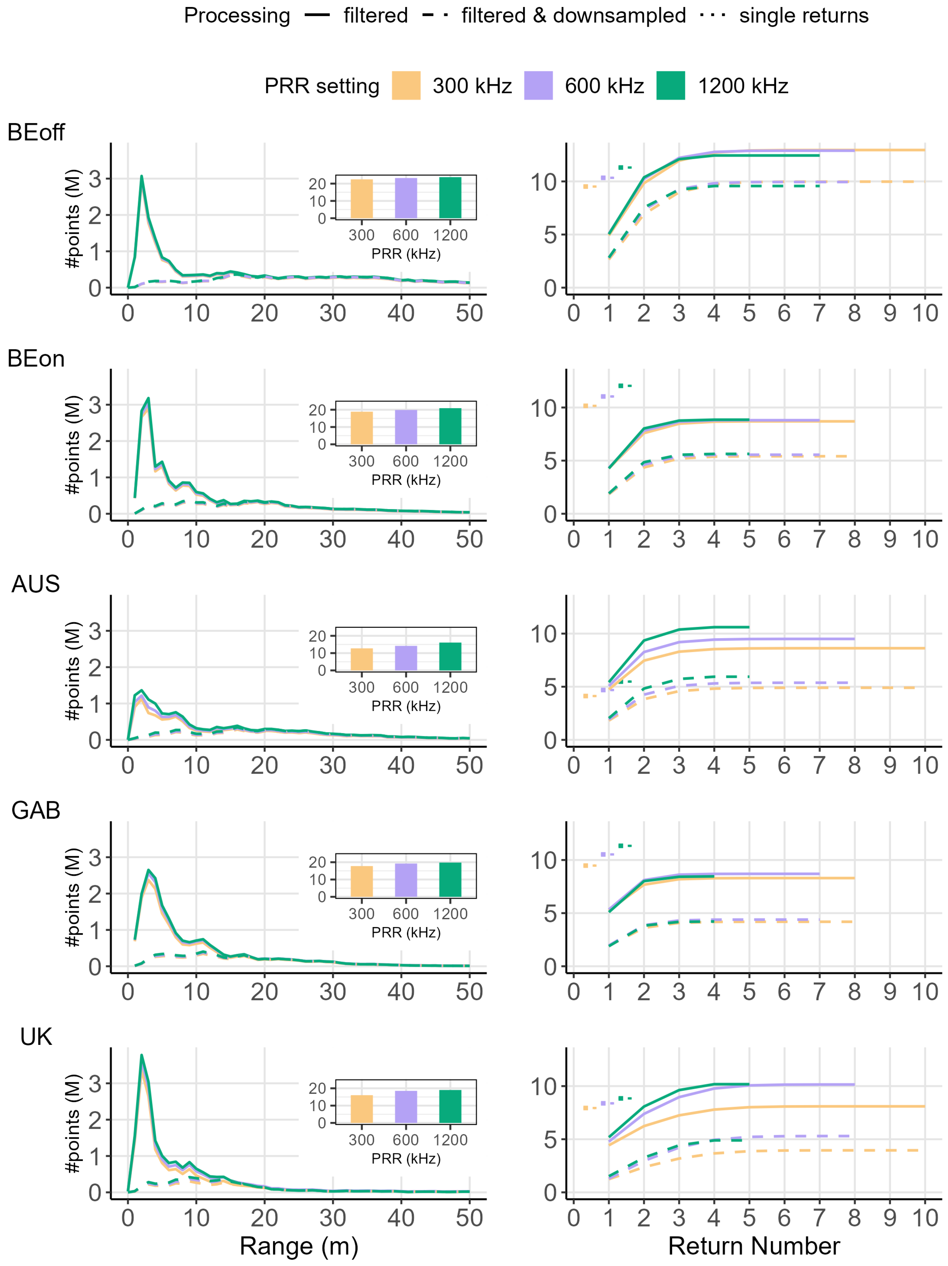
After the filtering step based on reflectance (<−17 dB) and deviation (>12), the distributions of two other metrics were investigated: the range from the scanner (m) and the return number (Figure 4). We observed that more raw returns were acquired for higher PRR replicates across the distributions. [Note: the increase in scan speed with PRR should emit the same number of pulses in each configuration.] For the range distribution, this effect was most noticeable in the first 20 m from the scanner. The biggest differences in raw returns found in the range distributions were among the replicates in the AUS plot. Furthermore, it clearly stood out that scans from higher PRR replicates consistently had a higher amount of first (single) return points compared to 300 kHz. In the BEoff plot, the difference in number of points was the smallest, indicating that the increase in points might be related to the presence of leaves. The AUS data showed the largest differences in return number between all the PRR replicates, whereas the difference between the 600 and 1200 kHz replicates tended to be lower in the other plots. The 300 and 600 kHz replicates had a significantly higher number of single returns compared to 1200 kHz, in agreement with the specifications of the manufacturer. While the amount of points at these higher return numbers was small compared to the total amount of points in a scan, they might be relevant in the context of occlusion.
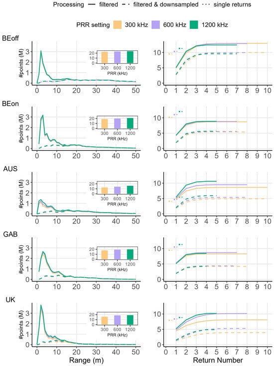
Figure 4.
Overview of the differences in the amount of remaining points in a single scan among the different pulse repetition rate replicates (PRR; 300, 600 and 1200 kHz) after the attribute filter step (top to bottom: BEoff, BEon, AUS, GAB, UK). The left side of the figure shows the amount of points in function of the range from the scanner, whereas the right side shows the number of points in each return number class (e.g., return number class 2 indicates the second hit from a laser beam). Both y-axes show the number of points in millions. The bar chart on the range plots indicates the total number of points in every PRR replicate. The return number graphs show the cumulative distribution of the points in function of the return number of the points. Thus, this shows the contribution of each consequent return number class on the total amount of points. This distribution is shown for both the filtered and the filtered + downsampled point clouds. At return number 1, the amount of single returns (no further hits) is indicated separately through the dotted lines.
The downsampling process thinned the point cloud, reducing the amount of points in all the forest types by up to 50%, which can be seen on the cumulative return number point distributions (Figure 4). The high peak in the first 10 m of the range distributions was completely removed after the downsampling step, removing much of the PRR-dependent differences seen in the raw range distribution (dashed versus full lines in Figure 4) below 15 m. Generally, above 15 m range the downsampling criteria were not met, so the point cloud remained unchanged. The patterns observed in the cumulative return number distributions generally remained similar before and after downsampling (the right panels in Figure 4), indicating that these patterns were likely related to spatial differences in points and not to point density differences (point density was largely evened out by the downsampling).
3.2. Impact of PRR on Individual Tree Point Clouds
3.2.1. Visual Occlusion and Point Density
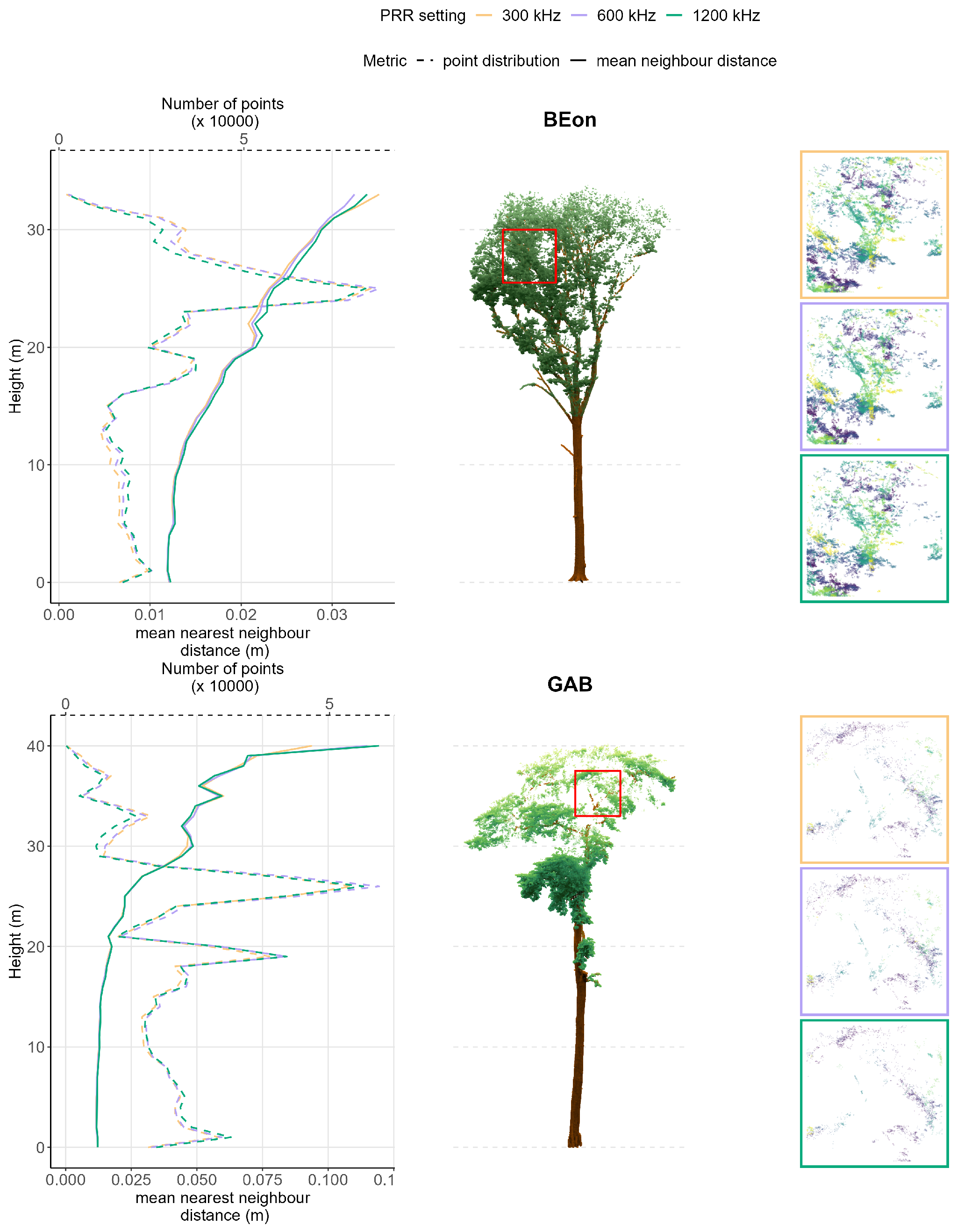
After these pre-processing steps, most individual tree point clouds from the different PRR replicates were nearly indistinguishable through visual inspection. The exceptions to this were the canopies in the point clouds from larger trees in forest plots with more complex understory vegetation and the dense canopies, mainly the BEon and GAB plot (Figure 5). In these canopies, a relatively high level of occlusion was present, due to occlusion from the understory, even in the 300 kHz PRR replicate. However, the occlusion was noticeably exacerbated in the higher PRR replicates in a way that allowed visual distinction among them. At lower heights, there was no noticeable increase in occlusion, independent of the vegetation complexity. The mean nearest neighbour distances consistently remained similar among the PRR replicates across the entire height range of the trees. The distributions of points across tree height reflected the visual observations that were made, as a noticeable decrease in the number of points in the canopies of certain large trees from higher PRR replicates was found, especially at 1200 kHz (left panel, Figure 5):
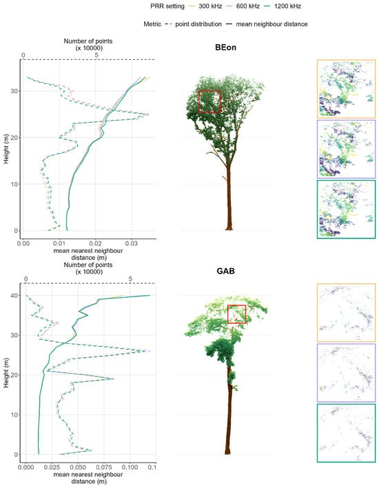
Figure 5.
Detailed overview of the final tree point cloud for the tallest tree in both the Beon and GAB plots. These are the tree point clouds after filtering, segmentation and 1 cm downsampling. The tree point clouds are plotted in the middle panel for visual reference. The left panel shows the distribution of the amount of points in the tree point cloud (dashed lines) as well as the mean nearest neighbour (four closest neighbours) distance (solid lines) in function of the height. The right panel shows a zoomed-in subset of a 5 m × 5 m × 5 m voxel from the tree canopies in each of the PRR replicates, to visually assess the occlusion impact of the PRR. The points in the zoomed-in subsets are coloured using the x-values (axis perpendicular to the plane), to better display depth. Overviews of the tallest trees from the other plots can be found in Appendix A Figure A2.
3.2.2. Individual Tree Metrics
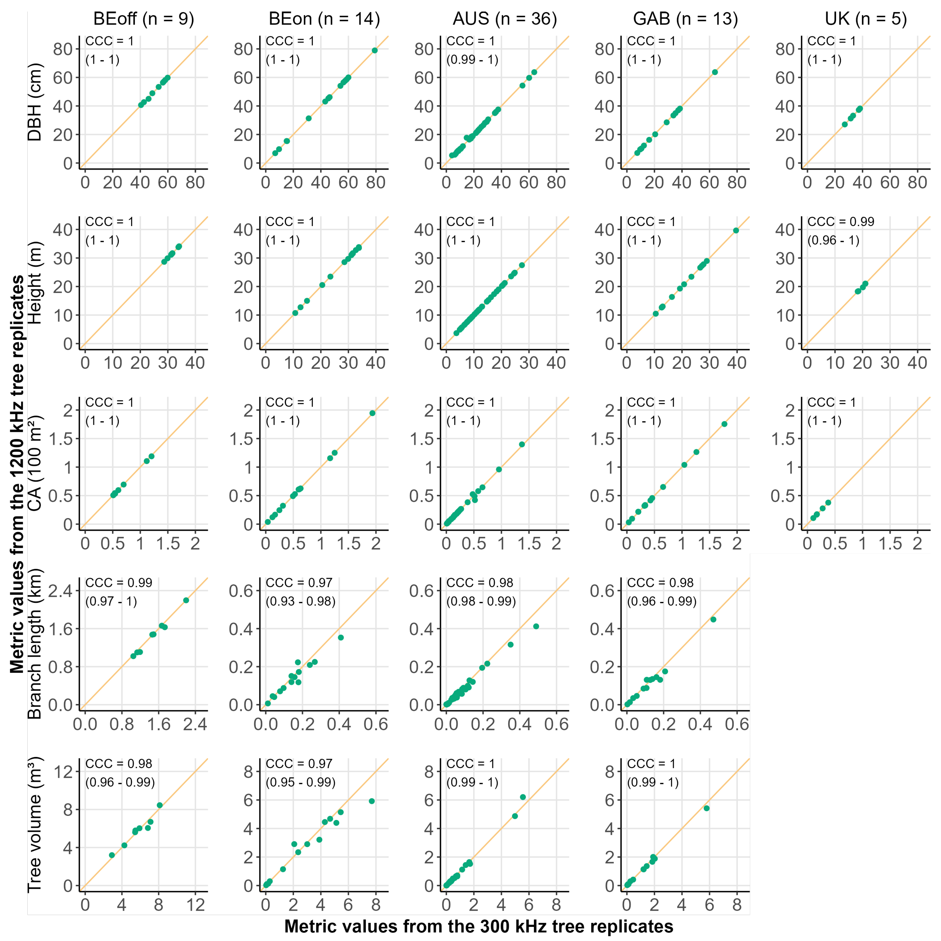
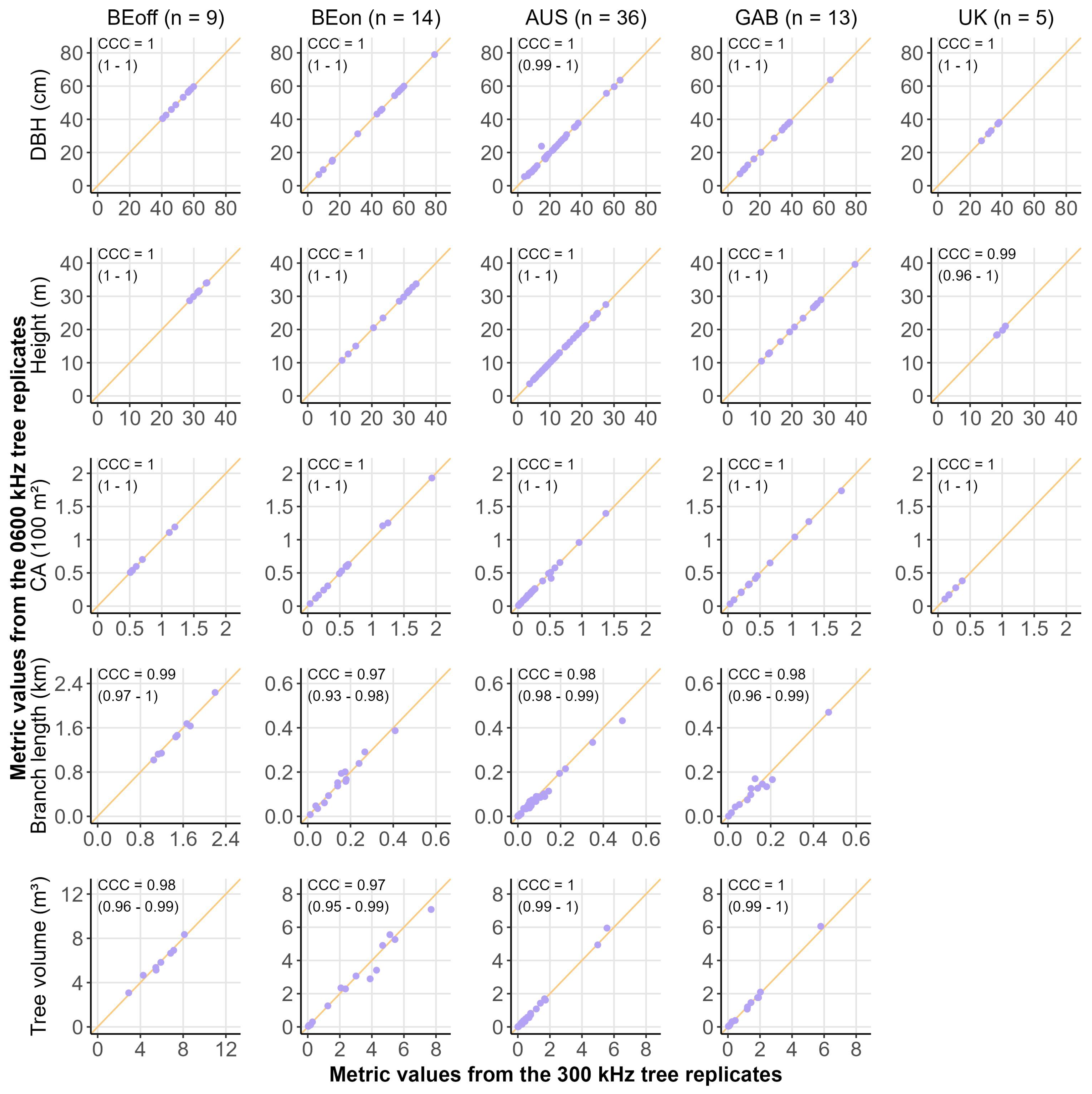
A resolute agreement was found between the structural metrics derived from all the PRR replicates (Figure 6). For all the selected metrics and across all the sampled forest types, a concordance correlation coefficient (CCC) higher than 0.96 was found between the replicates. For all metrics derived from the point clouds, the CCC values approached 1 when compared to both 600 kHz and 1200 kHz, indicating near-perfect agreement among all the PRR replicates. There was slightly more variability in the QSM-based metrics, but the agreement between the replicates remained very high (CCC confidence intervals ranging between 0.93 and 1). QSM-based metrics were not derived for the UK plot, due to high occlusion levels at all PRRs, preventing the construction of representative QSMs.
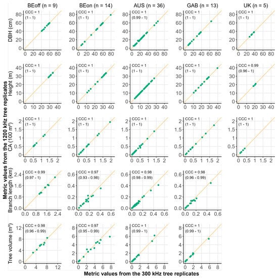
Figure 6.
Overview of the individual tree metrics for all plots; values extracted from the 300 kHz replicate are plotted as a reference versus the values from the 1200 kHz PRR replicate. The overview of the 300 kHz replicate metrics versus the 600 kHz replicate values can be found in Appendix A Figure A3. The plots are ordered in rows per structural metric (diameter at breast height DBH [cm], tree height H [m], crown projected area CPA [m2]), branch length BL [km] and total tree volume V [m3], respectively) and in columns per plot (BEoff, BEon, AUS, GAB, UK, respectively). The orange diagonal 1:1 line is plotted on every subplot. The concordance correlation coefficient (CCC) and its 95% confidence interval CI is given on every subplot, to demonstrate the agreement between the metric values from the 300 and 1200 kHz replicates.
4. Discussion
For the purpose of comparing the different PRR replicates, we used the 300 kHz data as a reference, since this setting has been most often used, historically [3,6]. However, it is important to note that this does not mean that the results from the 300 kHz replicate should be seen as the definitive best values. It is possible that data from higher PRR replicates can produce more accurate results in certain applications. For instance, it could be argued that a shorter scan time could lead to less co-registration errors, which, in turn, would improve the resulting QSMs. However, it is best practice to scan in no-to-minimal wind conditions, in order to ensure the quality of the 300 kHz replicate data as a benchmark. Overall, a quantitative assessment of wind impact on point cloud data is hard to achieve, and it is, to our understanding, also missing in the general literature of TLS in vegetated ecosystems.
We observed stark differences among the distributions of both reflectance and deviation within the different plots, but a relatively high similarity among the PRR replicates in each plot. The difference in the distributions among the plots appeared to be related to the forest structure and, more specifically, the canopy density and the presence of small objects (finer than beam diameter). The presence of such elements creates a high-scattering environment, with a high number of partial hits and reflections, which broadens the deviation peak.
The range data for the forest types sampled in this study had very low returns beyond 50 m, well within the maximum (or ambiguous) range for the PRRs used. The measurement configuration, driven by the sampling grid and occlusion considerations within the forest environment, inherently limited the mean target distance.
We found a high level of agreement among the structural metrics derived directly from the point clouds from the different PRR replicates (CCC values = 1). Within the QSM-derived structural metrics, the variation was larger but the results were still highly similar (CCC confidence intervals ranging between 0.93 and 1). The higher variability was expected, as the QSM process introduces a certain level of randomness [28] and also occurs when creating multiple QSM iterations using the exact same point cloud input.
The strong similarity among the structural metrics derived from each PRR replicate followed from the strong similarity in the respective point clouds. The various filtering and downscaling processing steps that were applied to the point cloud data throughout the workflow generally reduced the discrepancies in the point clouds between the PRR replicates. In these processing steps, the sections of the data where the PRR appeared to be having the largest impact were often removed, thus streamlining the PRR replicates. For example, relatively large differences between the PRR replicates can be observed in the reflectance distributions of the raw scan point clouds between −35 to −10 dB (Figure 3), most of which fell below the applied reflectance filter of −17 dB. The abovementioned filtering steps are standard practice in the processing of TLS point clouds, and the similarity in the point cloud replicates after filtering thus highlights the minimal impact of the PRR setting on the final point cloud quality in practical applications. Furthermore, the instances of visual increases in occlusion that we did find occurred inside the crowns within the dense canopies and were often foliage points. Due to the need for leaf removal before the QSM process, these areas of increased occlusion tend to be removed. The graph-based leaf–wood separation method [27] that was used in this study is also relatively conservative in its classification (personal observations during data processing), so the smallest branches are often classified as leaves and removed. It is in these smallest branches that the PRR would have the greatest effect, as we can see from the occlusion effects in the large trees. On the other hand, these smallest branches contribute the least to the overall tree volume and biomass, so their removal should have minimal effects on the total biomass estimates. Moreover, previous studies have found that the smallest branches in the upper canopy are often low quality [29] and can lead to an overestimation of tree volume from QSMs [6].
This study investigated the effect of the PRR on a selection of commonly derived single tree structure metrics, such as tree height or tree volume, often used in the context of aboveground biomass estimations. While we have demonstrated negligible effects on our selection of structural metrics within this context, we have not shown to what degree this applies to other types of applications. Within dense vegetation and tall tree canopies, some increased occlusion effects do occur at higher PRR settings. TLS data are commonly used in many other areas as well, such as the calculation of vegetation indices related to gap fraction [18,30], or radiative transfer modelling [31]. In the context of such applications, the effects of the higher PRR settings might have a more profound impact on the results.
Finally, our results demonstrate the general short-comings of TLS in certain forest types, due to occlusion. This was particularly the case for the dense conifer site in the UK, where we can see significant-to-drastic occlusion effects from as early as 10 m into the canopy. Beyond 10–12 m, stem points were virtually absent in most of the conifers, preventing the usage of QSMs beyond this point. This was true for all the PRR replicates, even the 300 kHz one, which we hypothesised was going to perform best in this type of location with high vegetation densities. This was unavoidable, due to the ground-based point of view of the TLS instrument. However, this work demonstrates high similarity in acquired data scanned using different PRRs, which suggests higher PRR settings can be used with minimal impact on derived tree structural metrics. The data collection time that can thus be saved by increasing the PRR creates opportunities to reduce the general occlusion issues associated with TLS. The time gain can, for instance, be used to increase the amount of scan locations in a fieldwork campaign. Combining higher PRR with higher angular scan resolutions is the subject of further ongoing work and has the potential to reduce occlusion in the upper parts of the canopy. A higher angular resolution means more outgoing laser pulses, and, therefore, an increased probability of high-quality (generally, pulses where the whole pulse footprint is hitting the target) and less occluded data in the upper canopy. However, an increase in angular resolution would increase scanning time again. It is, therefore, important to define clearly what is expected from the point cloud data, to make well-informed decisions before undertaking the fieldwork.
5. Conclusions
The results of this study demonstrate a high level of agreement among tree structural metrics derived from different PRR (laser pulse frequency) replicates in all plots, which indicates that higher PRRs can be used with little impact on the resulting point clouds, independently of the forest complexity. A potential check on the likelihood of a detrimental effect would be in the range data and whether it sits within the minimum to maximum/unambiguous range of the sensor. We have demonstrated that any PRR-induced effects on the point clouds are generally negated in the standard processing and have negligible effects on structural metrics derived at the tree level, including for metrics derived from QSMs, such as branch length and volume. The latter is especially promising in the context of AGB monitoring and the collection of TLS data on larger scales as calibration and validation AGB data in the context of EO missions. Using higher PRR settings would allow field crews to collect TLS data at higher speeds and, thus, potentially enable larger-scale campaigns. Perhaps even more importantly, it would enable TLS operators to more effectively capture the time windows of low wind conditions and, therefore, improve overall data quality. This would reduce the weather dependence of TLS data collection and create more certainty around data collection in wind-prone regions. The direct time gain of using a higher PRR could also be used to explore new scanning protocols to improve overall occlusion levels in TLS data, which presents an issue in many forest environments, regardless of the PRR, without impeding on the total duration of fieldwork campaigns. Such new protocols could include increasing the amount of scans acquired for a given area or changing other scanner settings, such as the angular resolution, which were previously undesired because of their impact on scan duration. Finally, it is important to note that the conclusions of this study largely apply to a selection of individual tree structural metrics that were chosen in the context of AGB estimation. Some slight differences between PRR replicates were found, specifically in areas that are already heavily occluded or contain a high number of scattering elements. This could potentially impact other types of TLS-derived metrics that were not tested in this study, so it remains good practice to consider the goals of the data collection when increasing the PRR.
Author Contributions
Conceptualization: T.E.V., K.C., H.V., A.B., M.D. and J.N.; methodology: T.E.V., K.C. and M.D.; software: T.E.V.; formal analysis: T.E.V.; investigation: T.E.V., K.C., B.D., L.T. and M.D.; resources: K.C. and A.B.; writing—original draft preparation: T.E.V.; writing—review and editing: all authors; visualization: T.E.V. and B.D.; supervision: K.C., H.V., J.N. and L.T.; project administration: K.C.; funding acquisition: K.C. All authors have read and agreed to the published version of the manuscript.
Funding
T.E.V. and data collection of the conifer stand in the UK was funded through the Climate Solutions Exchange’s BEAMS (Biocarbon Europe: Advancing Measurement Standards) project (www.csxcarbon.com). K.C. was funded by the European Union (ERC-2021-STG Grant agreement No. 101039795). The views and opinions expressed are, however, those of the author(s) only and do not necessarily reflect those of the European Union or the European Research Council Executive Agency. Neither the European Union nor the granting authority can be held responsible for them. The TLS data from Gabon were acquired with support from Innovate UK (project number 10004871).
Data Availability Statement
TLS data (individual tree point clouds and QSMs) and scripts (analysis and figures) are available at https://doi.org/10.5281/zenodo.10671784. The TLS data for the UK plot can be made available on request.
Acknowledgments
We thank TERN (Australia’s Terrestrial Ecosystem Research Network) for providing the infrastructure of the Cumberland Plain SuperSite. We thank Paul Green (NPL) for their useful suggestions and comments on the manuscript.
Conflicts of Interest
Authors Andrew Burt and Miro Demol were employed by the company Sylvera Ltd. The remaining authors declare that the research was conducted in the absence of any commercial or financial relationships that could be construed as a potential conflict of interest.
Abbreviations
The following abbreviations are used in this manuscript:
| TLS | terrestrial laser scanning |
| AGB | aboveground biomass |
| PRR | pulse repetition rate |
| QSM | quantitative structure model |
| EO | Earth Observation |
| DBH | diameter at breast height |
| H | tree height |
| CPA | crown projected area |
| V | total tree volume |
| BL | branch length |
| CCC | concordance correlation coefficient |
Appendix A
Appendix A.1
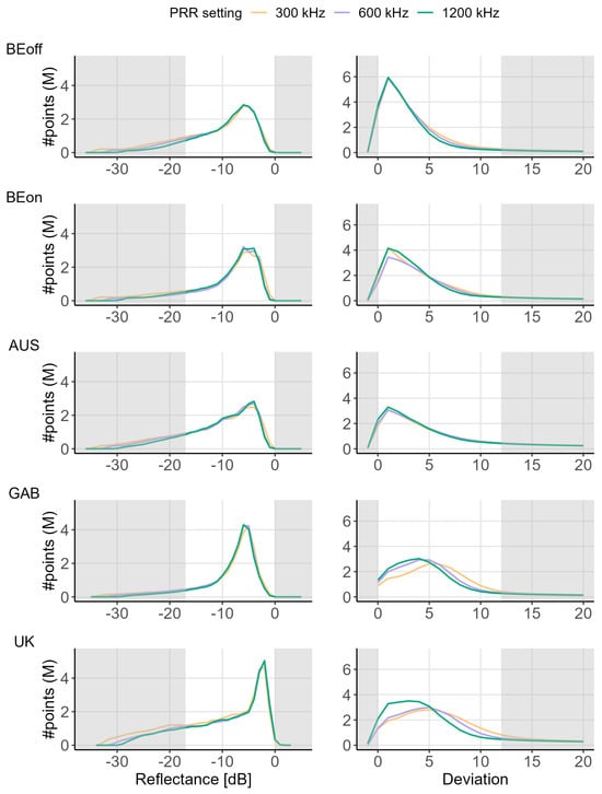
Figure A1.
Overview of the reflectance and deviation distributions in the raw data of a single tilt scan with different PRR settings. These are the tilt scans from the same scan locations as the upright scans from Figure 1 in Section 3.1. The deviation values are cut off at 20, but the values continue until 500+. The grey bands indicate the areas from the distributions that were filtered out in the processing, to remove high-uncertainty points.
Appendix A.2

Figure A2.
Detailed overview of the tallest tree in the BEoff, AUS and UK plot. The tree point clouds are plotted in the middle panel for visual reference. The left panel shows the distribution of the amount of points in the tree point cloud (dashed lines) as well as the mean nearest neighbour (four closest neighbours) distance (solid lines) in function of the height. The right panel shows a zoomed-in subset of a 5 m × 5 m × 5 m voxel from the tree canopy in each of the PRR replicates, to visually assess the occlusion impact of the PRR. The points in the zoomed-in subsets are coloured using the x-values (axis perpendicular to the plane), to better display depth.
Appendix A.3
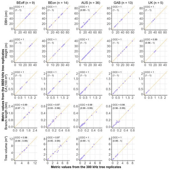
Figure A3.
Overview of the individual tree metrics for all plots; values extracted from the 300 kHz replicate are plotted as a reference versus the values from the 600 kHz PRR replicate, in the same way as Figure 5. The plots are ordered in rows per structural metric (DBH (m), H (m), CPA (m2), BL (m) and V (m3), respectively) and in columns per plot (BEoff, BEon, AUS, GAB, UK, respectively). The orange diagonal 1:1 line is plotted on every subplot. The concordance correlation coefficient (CCC) and its 95% confidence interval CI is given on every subplot, to demonstrate the agreement between the metric values from the 300 and 600 kHz replicates.
References
- Herold, M.; Carter, S.; Avitabile, V.; Espejo, A.B.; Jonckheere, I.; Lucas, R.; McRoberts, R.E.; Næsset, E.; Nightingale, J.; Petersen, R.; et al. The role and need for space-based forest biomass-related measurements in environmental management and policy. Surv. Geophys. 2019, 40, 757–778. [Google Scholar] [CrossRef]
- Disney, M.; Burt, A.; Calders, K.; Schaaf, C.; Stovall, A. Innovations in Ground and Airborne Technologies as Reference and for Training and Validation: Terrestrial Laser Scanning (TLS). Surv. Geophys. 2019, 40, 937–958. [Google Scholar] [CrossRef]
- Calders, K.; Verbeeck, H.; Burt, A.; Origo, N.; Nightingale, J.; Malhi, Y.; Wilkes, P.; Raumonen, P.; Bunce, R.G.H.; Disney, M. Laser scanning reveals potential underestimation of biomass carbon in temperate forest. Ecol. Solut. Evid. 2022, 3, e12197. [Google Scholar] [CrossRef]
- Calders, K.; Adams, J.; Armston, J.; Bartholomeus, H.; Bauwens, S.; Bentley, L.P.; Chave, J.; Danson, F.M.; Demol, M.; Disney, M.; et al. Terrestrial laser scanning in forest ecology: Expanding the horizon. Remote Sens. Environ. 2020, 251, 112102. [Google Scholar] [CrossRef]
- Calders, K.; Newnham, G.; Burt, A.; Murphy, S.; Raumonen, P.; Herold, M.; Culvenor, D.; Avitabile, V.; Disney, M.; Armston, J.; et al. Nondestructive estimates of above-ground biomass using terrestrial laser scanning. Methods Ecol. Evol. 2015, 6, 198–208. [Google Scholar] [CrossRef]
- Demol, M.; Wilkes, P.; Raumonen, P.; Krishna Moorthy Parvathi, S.; Calders, K.; Gielen, B.; Verbeeck, H. Volumetric overestimation of small branches in 3D reconstructions of Fraxinus excelsior. Silva Fenn. 2022, 56, 1. [Google Scholar] [CrossRef]
- Gonzalez de Tanago, J.; Lau, A.; Bartholomeus, H.; Herold, M.; Avitabile, V.; Raumonen, P.; Martius, C.; Goodman, R.C.; Disney, M.; Manuri, S.; et al. Estimation of above-ground biomass of large tropical trees with terrestrial LiDAR. Methods Ecol. Evol. 2018, 9, 223–234. [Google Scholar] [CrossRef]
- Momo Takoudjou, S.; Ploton, P.; Sonké, B.; Hackenberg, J.; Griffon, S.; de Coligny, F.; Kamdem, N.G.; Libalah, M.; Mofack, G.I.; Le Moguédec, G.; et al. Using terrestrial laser scanning data to estimate large tropical trees biomass and calibrate allometric models: A comparison with traditional destructive approach. Methods Ecol. Evol. 2018, 9, 905–916. [Google Scholar] [CrossRef]
- Duncanson, L.; Armston, J.; Disney, M.; Avitabile, V.; Barbier, N.; Calders, K.; Carter, S.; Chave, J.; Herold, M.; MacBean, N.; et al. Aboveground Woody Biomass Product Validation Good Practices Protocol, Version 1.0. 2021. Available online: https://lpvs.gsfc.nasa.gov/PDF/CEOS_WGCV_LPV_Biomass_Protocol_2021_V1.0.pdf (accessed on 2 December 2024).
- Wilkes, P.; Lau, A.; Disney, M.; Calders, K.; Burt, A.; Gonzalez de Tanago, J.; Bartholomeus, H.; Brede, B.; Herold, M. Data acquisition considerations for Terrestrial Laser Scanning of forest plots. Remote Sens. Environ. 2017, 196, 140–153. [Google Scholar] [CrossRef]
- RIEGL Laser Measurement Systems GmbH. 3D Terrestrial Laser Scanning System RIEGL VZ-i Series. Data Sheet, RIEGL VZ-400i, 2024/09/02. Available online: http://www.riegl.com/uploads/tx_pxpriegldownloads/RIEGL_VZ-400i_Datasheet_2024-09-02.pdf (accessed on 2 December 2024).
- Calders, K.; Armston, J.; Newnham, G.; Herold, M.; Goodwin, N. Implications of sensor configuration and topography on vertical plant profiles derived from terrestrial LiDAR. Agric. For. Meteorol. 2014, 194, 104–117. [Google Scholar] [CrossRef]
- Calders, K.; Disney, M.I.; Armston, J.; Burt, A.; Brede, B.; Origo, N.; Muir, J.; Nightingale, J. Evaluation of the Range Accuracy and the Radiometric Calibration of Multiple Terrestrial Laser Scanning Instruments for Data Interoperability. IEEE Trans. Geosci. Remote Sens. 2017, 55, 2716–2724. [Google Scholar] [CrossRef]
- Team, R.C. R: A Language and Environment for Statistical Computing; R Foundation for Statistical Computing: Vienna, Austria, 2013; Available online: http://www.R-project.org/ (accessed on 2 December 2024).
- Dowle, M.; Srinivasan, A. data.table: Extension of ‘data.frame’; 2023. Available online: https://rdrr.io/cran/data.table/ (accessed on 2 December 2024).
- CloudCompare. CloudCompare. 2022. Available online: https://www.cloudcompare.org/ (accessed on 2 December 2024).
- Burt, A.; Disney, M.; Calders, K. Extracting individual trees from lidar point clouds using treeseg. Methods Ecol. Evol. 2019, 10, 438–445. [Google Scholar] [CrossRef]
- Calders, K.; Origo, N.; Burt, A.; Disney, M.; Nightingale, J.; Raumonen, P.; Åkerblom, M.; Malhi, Y.; Lewis, P. Realistic Forest Stand Reconstruction from Terrestrial LiDAR for Radiative Transfer Modelling. Remote Sens. 2018, 10, 933. [Google Scholar] [CrossRef]
- Lowe, T.; Pinskier, J. Tree Reconstruction Using Topology Optimisation. Remote Sens. 2023, 15, 172. [Google Scholar] [CrossRef]
- Wilkes, P.; Disney, M.; Armston, J.; Bartholomeus, H.; Bentley, L.; Brede, B.; Burt, A.; Calders, K.; Chavana-Bryant, C.; Clewley, D.; et al. TLS2trees: A scalable tree segmentation pipeline for TLS data. Methods Ecol. Evol. 2023, 14, 3083–3099. [Google Scholar] [CrossRef]
- Roussel, J.R.; Auty, D.; Coops, N.C.; Tompalski, P.; Goodbody, T.R.; Meador, A.S.; Bourdon, J.F.; De Boissieu, F.; Achim, A. lidR: An R package for analysis of Airborne Laser Scanning (ALS) data. Remote Sens. Environ. 2020, 251, 112061. [Google Scholar] [CrossRef]
- Roussel, J.R.; Auty, D. Airborne LiDAR Data Manipulation and Visualization for Forestry Applications, R Package Version 3.1.2. 2021. Available online: https://github.com/r-lidar/lidR (accessed on 2 December 2024).
- Terryn, L.; Calders, K.; Åkerblom, M.; Bartholomeus, H.; Disney, M.; Levick, S.; Origo, N.; Raumonen, P.; Verbeeck, H. Analysing individual 3D tree structure using the R package ITSMe. Methods Ecol. Evol. 2023, 14, 231–241. [Google Scholar] [CrossRef]
- Lin, L.I.K. A Concordance Correlation Coefficient to Evaluate Reproducibility. Biometrics 1989, 45, 255–268. [Google Scholar] [CrossRef]
- Signorell, A. DescTools: Tools for Descriptive Statistics. 2023. Available online: https://cran.r-project.org/web/packages/DescTools/index.html (accessed on 2 December 2024).
- Burt, A.; Boni Vicari, M.; da Costa, A.C.L.; Coughlin, I.; Meir, P.; Rowland, L.; Disney, M. New insights into large tropical tree mass and structure from direct harvest and terrestrial lidar. R. Soc. Open Sci. 2021, 8, 201458. [Google Scholar] [CrossRef]
- Tian, Z.; Li, S. Graph-Based Leaf–Wood Separation Method for Individual Trees Using Terrestrial Lidar Point Clouds. IEEE Trans. Geosci. Remote Sens. 2022, 60, 1–11. [Google Scholar] [CrossRef]
- Raumonen, P.; Kaasalainen, M.; Åkerblom, M.; Kaasalainen, S.; Kaartinen, H.; Vastaranta, M.; Holopainen, M.; Disney, M.; Lewis, P. Fast Automatic Precision Tree Models from Terrestrial Laser Scanner Data. Remote Sens. 2013, 5, 491–520. [Google Scholar] [CrossRef]
- Abegg, M.; Boesch, R.; Schaepman, M.E.; Morsdorf, F. Impact of Beam Diameter and Scanning Approach on Point Cloud Quality of Terrestrial Laser Scanning in Forests. IEEE Trans. Geosci. Remote Sens. 2021, 59, 8153–8167. [Google Scholar] [CrossRef]
- Schraik, D.; Wang, D.; Hovi, A.; Rautiainen, M. Quantifying stand-level clumping of boreal, hemiboreal and temperate European forest stands using terrestrial laser scanning. Agric. For. Meteorol. 2023, 339, 109564. [Google Scholar] [CrossRef]
- Liu, C.; Calders, K.; Meunier, F.; Gastellu-Etchegorry, J.P.; Nightingale, J.; Disney, M.; Origo, N.; Woodgate, W.; Verbeeck, H. Implications of 3D Forest Stand Reconstruction Methods for Radiative Transfer Modeling: A Case Study in the Temperate Deciduous Forest. J. Geophys. Res. Atmos. 2022, 127, e2021JD036175. [Google Scholar] [CrossRef]
Disclaimer/Publisher’s Note: The statements, opinions and data contained in all publications are solely those of the individual author(s) and contributor(s) and not of MDPI and/or the editor(s). MDPI and/or the editor(s) disclaim responsibility for any injury to people or property resulting from any ideas, methods, instructions or products referred to in the content. |
© 2024 by the authors. Licensee MDPI, Basel, Switzerland. This article is an open access article distributed under the terms and conditions of the Creative Commons Attribution (CC BY) license (https://creativecommons.org/licenses/by/4.0/).


