Shallow Water Bathymetry Inversion Based on Machine Learning Using ICESat-2 and Sentinel-2 Data

Abstract

Shallow water bathymetry is essential for maritime navigation, environmental monitoring, and coastal management. While traditional methods such as sonar and airborne LiDAR provide high accuracy, their high cost and time-consuming nature limit their application in remote and sensitive areas. Satellite remote sensing offers a cost-effective and rapid alternative for large-scale bathymetric inversion, but it still relies on significant in situ data to establish a mapping relationship between spectral data and water depth. The ICESat-2 satellite, with its photon-counting LiDAR, presents a promising solution for acquiring bathymetric data in shallow coastal regions. This study proposes a rapid bathymetric inversion method based on ICESat-2 and Sentinel-2 data, integrating spectral information, the Forel-Ule Index (FUI) for water color, and spatial location data (normalized X and Y coordinates and polar coordinates). An automated script for extracting bathymetric photons in shallow water regions is provided, aiming to facilitate the use of ICESat-2 data by researchers. Multiple machine learning models were applied to invert bathymetry in the Dongsha Islands, and their performance was compared. The results show that the XG-CID and RF-CID models achieved the highest inversion accuracies, 93% and 94%, respectively, with the XG-CID model performing best in the range from −10 m to 0 m and the RF-CID model excelling in the range from −15 m to −10 m.

1. Introduction

Shallow bays and areas around islands and reefs are hotspots for human marine activities, and information on bathymetry is crucial for the study of these shallow seas. With the growth of the ocean economy and the increasing demand for the exploitation of resources such as fisheries, oil and gas, and marine tourism, knowledge of bathymetry is essential for safe navigation, harbor planning, and fishery resource assessments. These areas are also often important components of ecosystems, such as coral reefs and seagrass beds, and accurate bathymetric data can help to study their distribution and growth [1,2]. In addition, changes in bathymetry are closely linked to climate change, with rising sea levels due to global warming raising concerns about coastline retreat. Monitoring changes in bathymetry can also help to predict the extent of natural disasters such as tsunamis and hurricanes, supporting the mitigation of potential damage. The in-depth study of bathymetric information in shallow waters has significant scientific, economic, and social value [3,4,5].

Traditional shallow water bathymetric methods are divided into five main categories. (1) Sonar echo sounding techniques based on shipboard systems: These include single-beam echo sounding (SBES [6]) and multibeam echo sounding (MBES [7,8]). The former has a small coverage and low spatial resolution, while the latter provides detailed underwater topography through complete insonification of the area. (2) Bathymetry using airborne LiDAR data from non-imaging active remote sensing and satellite radar altimetry (e.g., SEASAT altimetry), with the former obtaining accurate measured depths in near-shore waters and the latter being suitable for only coarse, large-scale monitoring of seafloor topography changes. (3) Synthetic Aperture Radar (SAR) based on imaging active remote sensing for bathymetric inversion: When extracting seafloor features, this technique only identifies features with wavelengths similar to those of the local swell. If there is a large gap between the scale of the seabed topographic features and the wavelength of the waves, the effectiveness of the SAR technique will be limited [3]. (4) Bathymetric techniques based on imaging passive remote sensing: The use of satellite remote sensing images to establish bathymetric inversion models is divided into statistical and physics-based methods. Physics-based methods usually have higher accuracy, but need to consider complex optical properties; statistics-based methods analyze the relationship between spectral properties and depth through regression [9,10,11,12,13,14,15,16]. (5) Bathymetric inversion based on photogrammetry: This technique uses high-resolution satellite or airborne imagery to extract submerged features through advanced photogrammetric techniques. By applying stereo-matching and disparity estimation, this method reconstructs three-dimensional underwater topography. However, accurate refraction correction is essential for precise bathymetric data, and the technique is primarily applicable to shallow and ultra-shallow waters with depths up to 10 m [17,18,19,20,21]. Sonar and airborne LiDAR bathymetry are expensive and have limitations in remote and sensitive areas that are difficult to reach by ships and drones [22]. Photogrammetry can achieve high-resolution shallow water topography, but its depth capability is limited (typically up to 10 m). Satellite bathymetry allows for fast and cost-effective large-scale bathymetric inversion.

The research of satellite-derived empirical-based bathymetry (SDB) can be traced back to the 1970s and 1980s, when Polcyn et al. [23,24,25] proposed the SDB algorithm based on the band ratio, which gradually enabled the estimation of shallow water depths up to 5 m. Lyzenga et al. [26,27,28] simplified the classical radiative transfer equation to establish a quantitative relationship between the surface radiant energy and the water depth, thus simplifying the multispectral bathymetric inversion model and successfully estimated the water depth up to 15 m. Subsequently, Lyzenga et al. [29] proposed a multi-band linear model to correct optical attenuation and bottom reflection changes by log-transforming the blue and green band radiance combinations to improve the bathymetry accuracy, and Stumpf et al. [30] proposed an empirical ratio formula with only two unknown parameters, improving upon previous bathymetry inversion models. Experimental results demonstrated that the dual-band ratio model not only requires fewer parameters, but also performs well for low bottom depths and low reflectivity conditions. This model has become one of the classical approaches and forms the basis for many current studies. In recent years, scholars have made significant progress on the basis of these classical models. Pacheco et al. [31] improved the linear transformation algorithm of Lyzenga and inverted the nearshore SDB maps from Landsat 8 imagery. Hedley et al. [32] compared the ability of Sentinel-2 and Landsat 8 imagery in shallow water bathymetry and seabed mapping. With the development of machine learning technology, many researchers applied it to bathymetric inversion. Sandidge et al. [33] proposed a BP neural network for bathymetric inversion for the first time, and the effect exceeded traditional linear regression. Manessa et al. [34] used the random forest algorithm to carry out the bathymetric inversion of shallow coral reefs based on WorldView-2 imagery. Wang L et al. [35] used IKONOS-2 imagery and airborne LiDAR samples to implement bathymetric inversion by support vector machine model, while Wang Y et al. [5] improved the inversion accuracy by integrating spectral and spatial features through multilayer perceptron. Leng Z et al. [36] used the GRU deep learning model to carry out segmented bathymetric inversion of turbidity in Liaodong Bay. Ji X et al. [9] proposed an adaptive empirical method for different substrate types based on WorldView-2 imagery and multibeam echo sounding, airborne laser bathymetry (ALB) system. Knudby A et al. [12] compared five SDB models and discussed the importance of local neighborhood information for optimizing the effectiveness of bathymetric inversion. These studies have promoted the continuous development and application of SDB field, but satellite bathymetry still needs a large amount of in situ measured data to construct the mapping relationship between spectra and depth.

ICESat-2 (Ice, Cloud, and land Elevation Satellite 2) [22,37,38,39,40,41] was launched in September 2018 with the first on-board photon-counting lidar system, known as ATLAS (Advanced Topographic Laser Altimeter System). As a novel source of a priori bathymetry data, it makes up for the shortcomings of traditional satellite bathymetry that requires a large amount of measured data, and has been widely used in the field of Satellite-Derived Bathymetry (SDB) in recent years. Parrish et al. [42] successfully achieved 40 m bathymetry in clear waters using ICESat-2 data. Hsu H J et al. [43] combined ICESat-2 and Sentinel-2 data to achieve shallow water bathymetry of six islands in the South China Sea based on a semi-empirical model [30]. Chen Y et al. [44] proposed a photon-counting LIDAR bathymetry method based on adaptive variable ellipsoid filtering (AVEBM) and verified the accuracy in Yongle Atoll and Chilianyu Archipelago. Xie C et al. [45] applied the density clustering algorithm (DBSCAN) to remove noise from ICESat-2 raw photons and combined them with Sentinel-2 data to perform bathymetric inversion, demonstrating the potential of combining data from multiple sources. Peng K et al. [46] proposed a physically assisted convolutional neural network (PACNN) model based on convolutional neural networks (CNNs) by linking Sentinel-2 and ICESat-2 data for shallow water bathymetry. Guo X et al. [47] performed bathymetric inversion by integrating ICESat-2 and Sentinel-2 data using a BP neural network model, which effectively enhanced the bathymetric inversion results. Xie C et al. [11] fused ICESat-2 and Sentinel-2 data and incorporated a radiative transfer-based model into a convolutional neural network (CNN) for bathymetric inversion, significantly improving inversion accuracy and further validating the effectiveness of multi-source data fusion.

This study aims to propose a simple and convenient method for shallow water depth inversion based on satellite datasets, enhancing the performance of the water depth inversion model through the integration of various types of information. First, the feasibility of applying ICESat-2 data in shallow water bathymetry is explored and improved. To this end, we developed a fully automated script capable of extracting water depth photons, where users only need to define the study area and select high-quality ICESat-2 data tracks and dates. Second, this study uses the information from the red, green, and blue bands of Sentinel-2 data as spectral feature information, the Forel-Ule index (FUI) [48,49,50] as water color information, and normalized latitude and longitude coordinates, along with polar coordinates, as spatial information. These are combined with the extracted ICESat-2 water depth point data to train the traditional Stumpf model, Polynomial Regression model, Random Forest model, Gradient Boosting model, and XGBoost model for water depth inversion. Through a comprehensive analysis of the accuracy and applicability of each model in shallow water bathymetry, this study provides new perspectives and methodologies for the effective application of ICESat-2 and Sentinel-2 data in shallow water depth inversion.

2. Materials and Methods

2.1. Study Area and Data

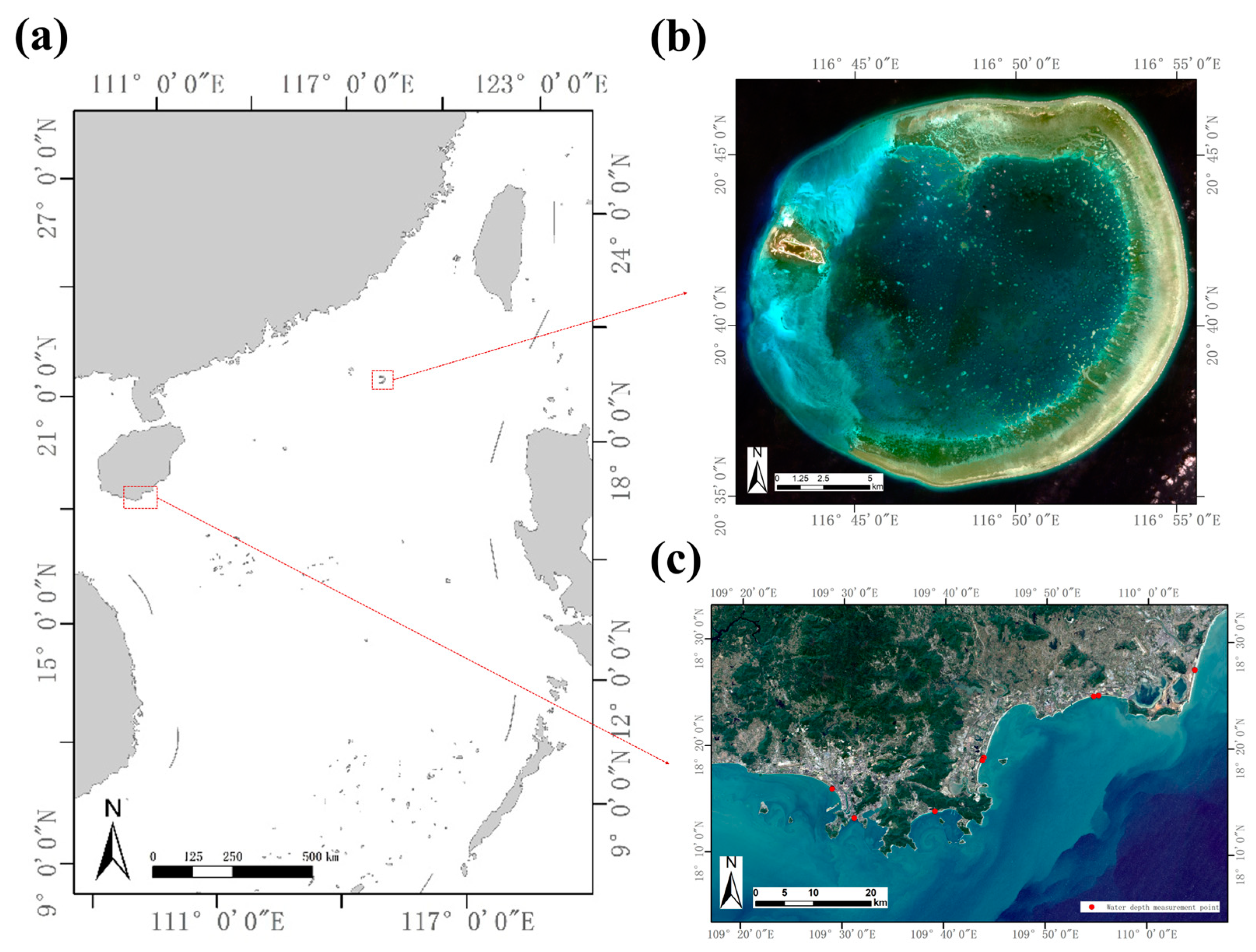
2.1.1. Study Area and In Situ Bathymetric Data

The first study area is located in the shallow coastal regions of Clearwater Bay, Haitang Bay, and Yalong Bay (Lingshui-Sanya Bay) in Hainan Province, China, situated in the southeastern part of the province within a low-latitude coastal zone, as shown in Figure 1a. The in situ data consist of 24 bathymetric points collected in 2020, which are used to evaluate the bathymetric capability of ICESat-2 data. The locations of these measurement points are indicated by red dots in Figure 1c.

The second study area is located in the Dongsha Islands (Figure 1b), a group of islands and reefs in the northern part of the South China Sea. It consists of 11 coral reefs and 35 islands with a total area of about 0.57 km². The Dongsha Islands are the furthest group of islands in the South China Sea from Hainan, about 350 km from Hainan Island and about 460 km from the Leizhou Peninsula in Guangdong Province. These islands consist mainly of coral reefs and sandy islands with low reliefs and small islands. The natural environment of the Dongsha Islands remains relatively pristine, with a well-preserved ecosystem. Covering a total sea area of approximately 5000 km², the Dongsha Islands feature a comprehensive topography that includes unique natural formations such as reef flats, lagoons, sandbars, shoals, channels, and islands, making it a quintessential example of an atoll landform.

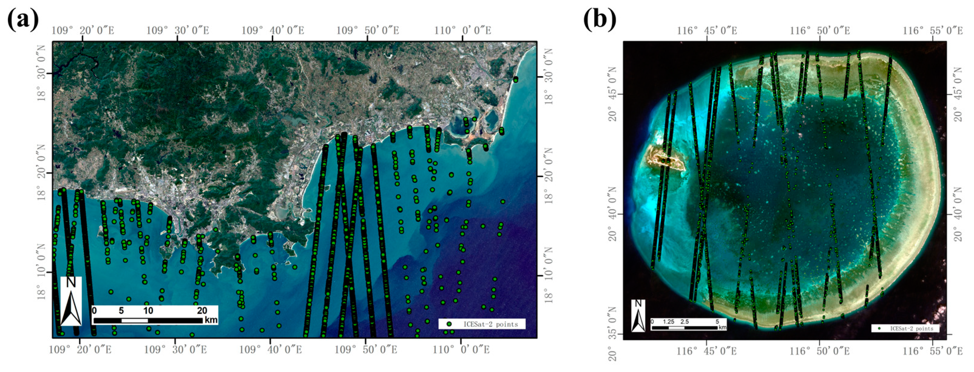
2.1.2. ICESat-2 Data

ICESat-2 (Ice, Cloud, and Land Elevation Satellite-2) is an Earth observation satellite launched by NASA in September 2018, designed to accurately measure changes in surface elevation through laser altimetry to support global environmental monitoring and climate change research. ICESat-2 carries the Advanced Topographic Laser Altimeter System (ATLAS), one of the most advanced laser altimeters in Earth’s orbit to date. ICESat-2’s primary mission includes assessing volumetric changes in the polar ice caps in order to establish an active monitoring system related to sea level change and ocean circulation impacts. In addition, ICESat-2 is used to measure global vegetation characteristics, land topography, and the backscattering properties of molecules, clouds, and aerosols in the atmosphere. These data are critical to understanding global change and supporting environmental protection [51,52,53,54,55,56,57,58]. The ATLAS uses six laser beams divided into three pairs, each consisting of a strong beam and a weak beam. The strong beam has four times the energy of the weak beam, a design that helps to obtain stable data under varying albedo conditions. The distance between each pair of laser pulses is 90 m, while the distance between each pair and the next is 3.3 km. This spatial configuration strikes a balance between high-resolution sampling and wide area coverage, enabling ICESat-2 to capture detailed altimetry data across diverse global surfaces with improved accuracy.

ICESat-2 provides a variety of data products, and the Level 2 data of ICESat-2, ATL03 (Global Geopositioning Photonics Data), was used in this study (as shown in

Table 1. Data table of ICESat-2 and Sentinel-2 in the study area.

Site	Lingshui-Sanya Bay	Dongsha Islands
Latitude	18°3.84′N–18°33.3′N	20°34.75′N–20°47.20′N
Longitude	109°17.1′E–110°7.8′E	116°41.34′E–116°55.61′E
ICESat-2 Data	ATL03_20200130213819_05370607_006_01 ATL03_20200427052044_04840701_006_02 ATL03_20200430171804_05370707_006_02 ATL03_20200530034826_09870701_006_01 ATL03_20200727010031_04840801_006_01 ATL03_20200828232813_09870801_006_01 ATL03_20200901112535_10400807_006_02 ATL03_20200930100134_00950907_006_02 ATL03_20210502234906_05981107_006_01 ATL03_20210524103607_09261101_006_01 ATL03_20210524103607_09261101_006_01 ATL03_20220624154329_00421601_006_01 ATL03_20220628034053_00951607_006_01 ATL03_20220829004446_10401607_006_01	ATL03_20190129144159_04910207_006_02 ATL03_20190730060118_04910407_006_02 ATL03_20191021135212_03770501_006_02 ATL03_20191029014115_04910507_006_01 ATL03_20200420051144_03770701_006_02 ATL03_20200427170047_04910707_006_02
Sentinel-2 Data	S2A_MSIL2A_20201203T031109_N0500_R075_T49QCA_20230303T030821	S2A_MSIL2A_20240222T023721_N0510_R089_T50QMH_20240222T061746

). The ATL03 dataset consists of all the raw photon data recorded in six different trajectories (three strong beams and three weak beams), each with unique latitude, longitude, and elevation angles based on the WGS84 ellipsoidal datum with unique latitude, longitude, and elevation angles. The dataset is corrected for atmospheric delays, solid tides, and systematic pointing biases, but does not correct for bathymetric errors such as water surface fluctuations, tilted surfaces, and water column effects. Although the ATL03 dataset provides detailed photon data, due to the high sensitivity of the detector, the data contain a large number of noise photons, especially in the daytime solar background. In order to distinguish between signal and noise photons, the ATL03 dataset introduces a ‘confidence’ parameter ranging from 0 to 4, where the higher the confidence, the more likely the photon is a signal. However, due to attenuation and scattering effects in the water column, the distributions of signal and noise photons are different from those in the atmosphere, resulting in poor performance of the confidence parameter in undersea signal photon detection [42]. Therefore, this study proposes a density-based signal detection algorithm to filter the photons and identify the water depth signal photons.

2.1.3. Sentinel-2 Data

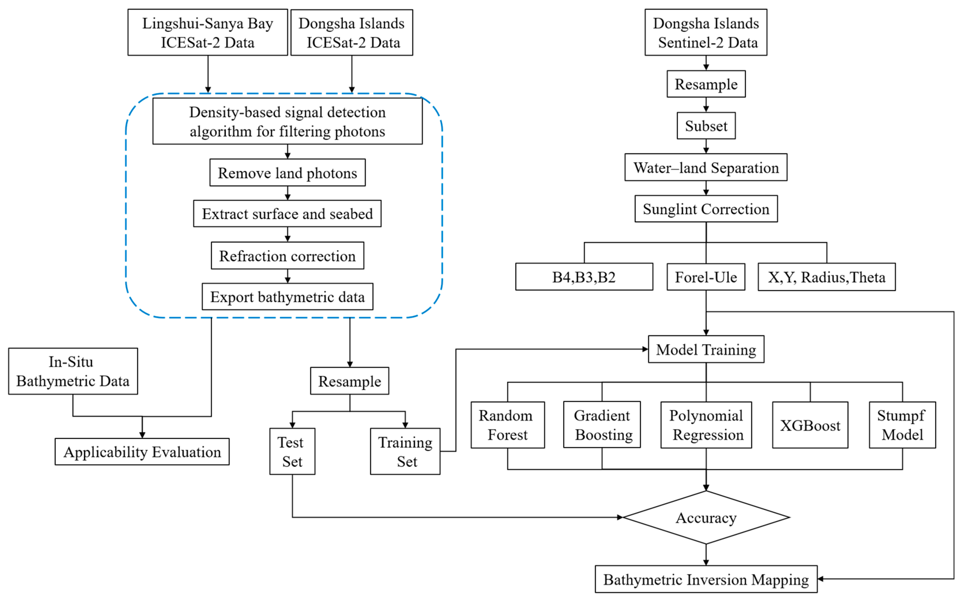
Sentinel-2 [59] is a key satellite in the European Space Agency’s (ESA) Copernicus program, designed to monitor the Earth’s surface through high-resolution optical imaging. The Sentinel-2 satellites, comprising Sentinel-2A and Sentinel-2B, were launched in June 2015 and March 2017, respectively. Sentinel-2’s L2A-level data are radiometrically calibrated and atmospherically corrected surface reflectance images specifically designed for detailed surface analyses. The L2A class data are processed from the original Level-1C data (geometrically corrected orthophotos). It is characterized by high spatial resolution and multi-spectral coverage. Sentinel-2 L2A level data provides resolutions of 10, 20, and 60 m. The resolution varies by band, with the 10-meter resolution band being suitable for detailed surface analysis. Coverage of 13 spectral bands, ranging from visible to near-infrared (VNIR) and short-wave infrared (SWIR), provides rich spectral information to support a wide range of applications.

The Sentinel-2 L2A level data for this study was obtained from the European Space Agency’s (ESA) Copernicus Open Access Hub. The data are projected using the UTM/WGS84 (Universal Transverse Mercator/World Geodetic System 84) projection, which facilitates its use in conjunction with other Geographic Information System (GIS) data (data table shown in Table 1).

2.2. Methodology

The main work of this study involves the following aspects: First, bathymetric measured data from Lingshui-Sanya Bay, as well as ICESat-2 data and Sentinel-2 images from both Lingshui-Sanya Bay and Dongsha Islands, were obtained. Second, Sentinel-2 images of the two study areas were preprocessed, and ICESat-2 bathymetric photon signals were extracted using a fully automated script. In the Lingshui-Sanya Bay area, ICESat-2 bathymetric photon data were matched with measured bathymetric data in terms of coordinates to evaluate the feasibility of ICESat-2 data for bathymetric applications. Subsequently, ICESat-2 bathymetric photon data from Dongsha Islands were resampled to a 10 m resolution and matched with Sentinel-2 images to obtain the red, green, and blue band reflectance values of the ICESat-2 bathymetric points. Additionally, the dataset was augmented with the FUI to represent water color information and spatial information, including normalized latitude and longitude coordinates as well as polar coordinates (radius and angle). Using this comprehensive dataset, the Stumpf model, Polynomial Regression model, Random Forest model, Gradient Boosting model, and XGBoost model were trained to invert the bathymetry of the Dongsha Islands. Finally, the accuracy and applicability of each model were comparatively evaluated. Figure 2 illustrates the technical workflow of this study.

2.2.1. Lingshui-Sanya Bay Measured Data Acquisition

On 15–16 August 2020, our team carried out a field collection of seawater depths in Lingshui-Sanya Bay. This study used the bathymetric rod method, which measures the distance from the seafloor to the water surface by inserting a bathymetric rod vertically into the seawater and measuring the distance from the seafloor to the water surface through the scale marked on the rod. The bathymetric rod detection method is widely used in marine scientific research because of its simplicity and practicality. We used this method to detect a total of 24 discrete points of seawater bathymetry data in Lingshui-Sanya Bay, and tidally corrected the measured data by checking the tide tables of the harbors near the measured points, as shown in

Table 2. In situ bathymetry data sheet.

Longitude	Latitude	Distance from Shore (m)	Measured Water Depth (m)	Tide-Corrected Water Depth (m)	Time
110.07672	18.45667	23.7	0.1	0.5	11:49
110.07676	18.45665	27.4	0.6	1	11:49
110.07686	18.45660	39.1	1.1	1.5	11:52
109.91875	18.41580	57.8	0.1	1.02	16:50
109.91877	18.41569	70.5	0.46	1.38	16:50
109.91878	18.41562	78.1	1.1	2.02	16:53
109.91078	18.41475	85.8	0.1	1.02	17:12
109.91079	18.41464	97.5	0.4	1.32	17:13
109.91082	18.41454	109.4	1.1	2.02	17:15
109.73072	18.31802	11.8	0.1	0.78	18:24
109.73077	18.31799	18.9	0.4	1.08	18:25
109.73118	18.31777	67.4	1.1	1.78	18:30
109.72836	18.31361	32.1	0.1	0.78	18:41
109.72848	18.31354	46.1	0.4	1.08	18:42
109.72884	18.31329	93.2	1.1	1.78	18:47
109.65143	18.23303	15.2	0.1	0	10:17
109.65143	18.23300	18.5	0.5	0.4	10:18
109.65144	18.23284	36.4	1	0.9	10:22
109.51883	18.22201	15.8	0.1	0.97	14:24
109.51884	18.22172	48.2	0.3	1.17	14:25
109.51886	18.22095	133.9	0.9	1.77	14:32
109.48227	18.26732	40.2	0.1	1.01	15:07
109.48217	18.26719	57.2	0.4	1.31	15:08
109.48197	18.26691	95.5	1	1.91	15:13

.

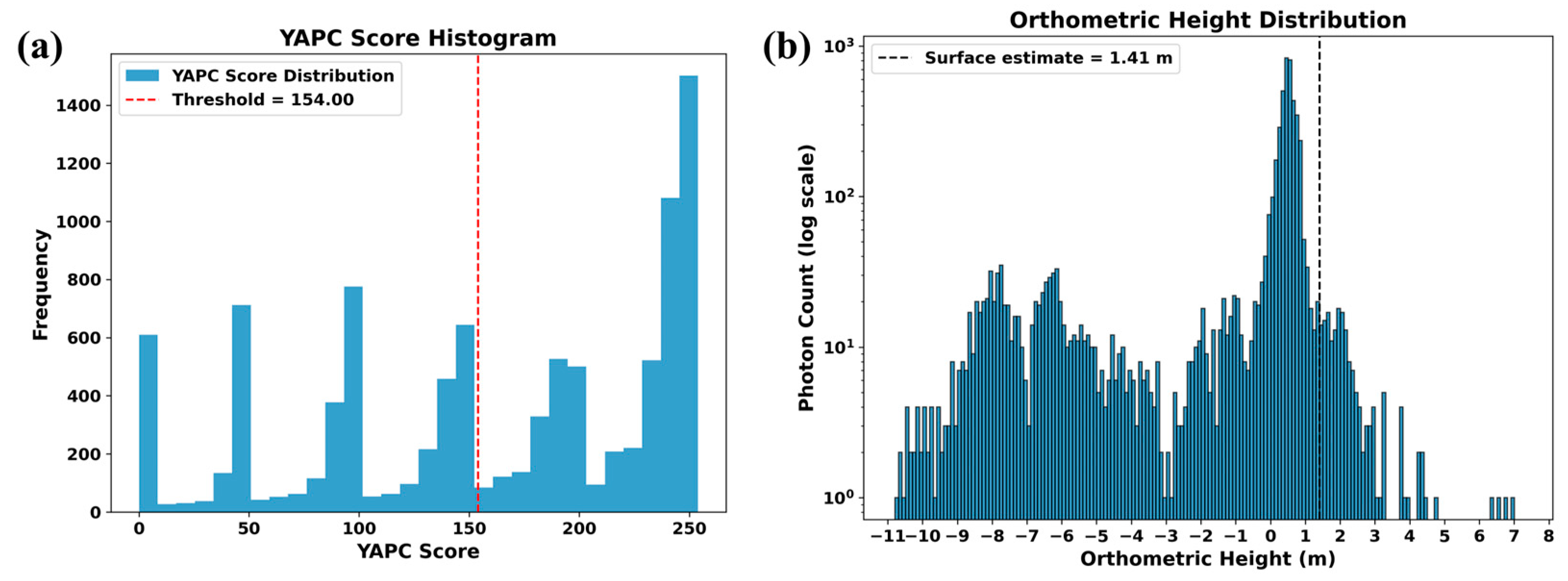
2.2.2. ICESat-2 Data Preprocessing

Our main objective was to extract the bathymetric photon signals from ICESat-2 satellites and compare them with the measured data of Sanya Bay, and then to evaluate the accuracy and reliability of the extraction method of ICESat-2 data bathymetric photon signals used in this study, taking into account the hydrographic characteristics of Sanya Bay. The specific data processing steps include data acquisition, signal filtering, land photon removal, water surface and seafloor extraction, refraction correction, and the exportation of bathymetric data, as shown in the blue box in Figure 2.

In this study, we referred to the methodology provided by the 2023 ICESat-2 Hackweek (https://icesat-2-2023.hackweek.io/tutorials/bathymetry/bathymetry_tutorial.html (accessed on 24 February 2024)) [60] to write a script that automatically extracts water depths in batch based on the date and orbit number of ICESat-2 data within the study area. Before running the script, we just needed to determine the study area extent and filter out the orbits and dates with good data quality. Using OpenAltimetry ICESat-2 Webpage (https://openaltimetry.earthdatacloud.nasa.gov/data/icesat2/ (accessed on 24 February 2024)), we could select the region of interest. By modifying the date and orbit number, we could select photon data orbits with good quality, density, and regular point clouds. By inputting the selected orbit, date, and the latitude and longitude of the study area into the script and running it, the water depth signal photons for the study area were automatically filtered. The following describes the main workflow and theoretical methods of the script.

Our study utilized the Python library “Sliderule” and an EarthData account to download the ATL03 data corresponding to specific latitude, longitude, date, and orbit numbers of the study area. ICESat-2, equipped with a laser altimeter system, conducts high-precision measurements of the Earth’s surface, generating point cloud data that include ground and water surface elevations. To ensure that the ICESat-2 orbital data acquired covers the target area’s laser detection information, we employed the distribution preview feature of the ATL08 dataset to identify orbits that potentially contain high-quality signals. After the data was downloaded, we proceeded with the filtering of photon signals. The ATL03 product provided by ICESat-2, along with the “Sliderule” tool, encompasses a variety of photon signal measurement and processing techniques. In this study, we utilized the YAPC (Yet Another Photon Classifier) algorithm, which was developed by NASA researchers [61]. The YAPC algorithm is a density-based signal detection method that identifies valid signals by analyzing the spatial distribution of photon signals. Compared to traditional photon classification approaches, YAPC exhibits heightened sensitivity to environmental variations, enabling it to adapt more accurately to the characteristics of diverse water bodies. Utilizing the YAPC algorithm, we filtered and identified effective photon signals. Taking the processing of ATL03_20190129144159_04910207_006_02 data as an example, Figure 3a presents a photon signal density confidence map based on the YAPC algorithm, illustrating the spatial distribution of photon signals along the track. Different colors in the figure represent photon signals of varying density levels, with signals of higher confidence indicated by more prominent colors. To determine the minimum threshold for valid signals, we employed the Otsu [62] thresholding method for automatic acquisition (Figure 4a). Photons with YAPC signal scores above this threshold are considered valid signals. Subsequently, we excluded land photons from the valid signals. To achieve this, we constructed a histogram to tally the frequency of photon occurrences across various height intervals, ranging from −50 m to 50 m with a step size of 0.1 m. By identifying the height value with the highest frequency in the histogram (i.e., the most common photon height), we estimated the water surface height. To account for the effects of waves or surface undulations, we added a 1 m buffer to this height. The vertical black line in Figure 4b represents the estimated water surface height; photons above this height were considered land photons and were removed, while valid photons below this height were classified as water area photons (Figure 3b). Building on this foundation, we extracted the water surface and seafloor from the remaining water area photons. We performed binning on the spatial distribution of photon signals, setting the resolution along the track to 20 m. Based on the distribution of photon density, we adaptively adjusted the height resolution and generated a two-dimensional histogram. The binning operation aimed to divide the photon data into multiple intervals along both the height and track dimensions, facilitating the analysis of photon height distribution characteristics. To enhance the detection of signal peaks, we applied adaptive filtering to the generated two-dimensional histogram. The filtering strength was dynamically adjusted based on local variance to smooth the signal and reduce the impact of noise, thereby highlighting the main peaks of the signal. Subsequently, based on the peak values of each waveform, we assumed that the topmost return signal represents the water surface. After removing the water surface peak, we selected the prominent peak as an indicator of seafloor depth, extracting water surface and seafloor return information from the photon height histogram. After acquiring the water surface and seabed depth, we proceeded with refraction correction based on the research outcomes of Parrish et al. [42] in 2019, which effectively enhances the precision of bathymetric measurements. Subsequently, we iteratively traversed each waveform, extracted the water surface and seabed information, applied refraction correction (Figure 5), calculated the water depth, and compiled the ICESat-2 bathymetric signal extraction results for the area.

Suitability assessment of processed ICESat-2 bathymetric data. The bathymetric performance of the ICESat-2 satellite data were evaluated by matching and comparing with the existing Lingshui-Sanya Bay bathymetry data. Firstly, the bathymetric real measurements were coordinate-matched with the extracted Lingshui-Sanya Bay ICESat-2 bathymetry data. For each measured point, the K Nearest Neighbours algorithm (KNN) was used to find the five nearest ICESat-2 data points, and the difference in bathymetry between these points and the measured points was computed, using the Root Mean Squared Error (RMSE), MeanDepthDiff, Variance of Depth Difference (VarDepthDiff), and Mean Squared Error (MSE) to quantify the differences to assess the consistency and error of the data. Additionally, the average distance to the five nearest ICESat-2 points was calculated to further assess the spatial distribution and proximity of the ICESat-2 points relative to the measured locations.

2.2.3. Sentinel-2 Image Preprocessing

Pre-processing the Sentinel-2 L2A data was an important step in constructing models for remote sensing analyses. Although the L2A data have been atmospherically corrected to generate surface reflectance data, there are still some necessary preprocessing steps before specific analyses can be performed.

Sentinel-2 L2A data were acquired from the Copernicus Open Access Hub (https://dataspace.copernicus.eu/ (accessed on 24 February 2024)), selecting high-quality imagery with minimal cloud cover. After resampling to 10 m resolution using SNAP, the images were cropped to the study area. Water bodies were extracted using a mask based on the near-infrared band (B8) with the formula (If B8 > 0.05, then NaN, else 1) [63]. Sunglint correction [64] was applied using the Deglint processor in the Sen2Cor plugin to reduce surface reflections, enhancing water body analysis accuracy.

Finally, consistency between ICESat-2 bathymetric data and Sentinel-2 imagery was ensured. To achieve spatial consistency, the ICESat-2 bathymetric data points were first mapped to the nearest grid cell in a 10 m resolution raster coordinate system. Data cleaning was then performed to ensure consistency: each RGB combination was checked against its corresponding depth value to ensure a unique depth value for each RGB combination. Additionally, it was verified that each depth value corresponded to a unique RGB combination, preventing the association of a single depth value with multiple RGB combinations. This process ensured that each raster cell was associated with only one depth value, providing a consistent data foundation for subsequent analysis.

2.2.4. Bathymetric Inversion Model for the Dongsha Islands

With the development of satellite remote sensing technology, bathymetric inversion using satellite images has become a fast and economical alternative to traditional bathymetry. Machine learning algorithms are good at learning complex nonlinear relationships from large amounts of data, which can significantly improve the accuracy of bathymetric inversion. This section describes the use of four machine learning methods, Random Forest, Gradient Boosting, XGBoost, and Polynomial regression, to train bathymetric inversion models based on spectral feature information, water body color information, and spatial location data. The performance of these models is compared with the improved logarithmic band ratio algorithm proposed by Stumpf et al. [30] in 2003 to explore the application of machine learning in satellite-derived bathymetry.

Creation of a Comprehensive Information Dataset

In the previous section, we obtained the ICESat-2 bathymetric dataset after data consistency processing. The ICESat-2 bathymetric points were matched with Sentinel-2 imagery, and the reflectance values of the red, green, and blue bands corresponding to each bathymetric point were extracted. These reflectance values were used as spectral feature information.

The Forel-Ule Index (FUI) is a classic index used to characterize the color of water bodies, primarily assessing the optical properties and water quality. In this study, we adopted the FUI algorithm developed by Van der Woerd H. J. and Wernand M. R. in 2018 for Sentinel-2 imagery [48], using the obtained FUI values as water color information.

Previous studies [5,65] have shown that incorporating spatial location information can improve the accuracy of bathymetric inversion using machine learning. However, these studies typically considered only the X and Y coordinates of the pixels, without accounting for polar coordinates. Polar coordinates provide additional spatial features, such as distance and angle, which are more sensitive to areas with non-uniform data distribution. In this study, spatial location information was enhanced by introducing polar coordinates alongside the traditional normalized pixel coordinates (X, Y). Specifically, for each pixel’s normalized coordinates, the distance (R) and angle (θ) from the bottom left corner of the image were calculated.

The integrated dataset includes the three aforementioned components of feature information. Before model training, data standardization [Equation (1)] was applied to address potential issues arising from discrepancies in the scale and range of different features. Without standardization, features with larger numerical ranges could dominate the training process, overshadowing other important variables. Additionally, significant differences in feature scales could impede the convergence of gradient-based optimization algorithms, ultimately reducing training efficiency. This standardization ensured consistent value ranges across the different features, thereby improving the training performance and predictive accuracy of the model.

$$X_{\mathrm{standardized}}={\displaystyle \frac{X-\mu }{\sigma }}$$

(1)

where $X$ is the original data, $\mu$ is the mean of the feature, $\sigma$ is the standard deviation of the feature, and $X_{\mathrm{standardized}}$ is the standardized data. Through this standardization process, the data distribution is adjusted to a normal distribution with a mean of 0 and a standard deviation of 1.

Model Training

In this study, we use the integrated information as features and the ICESat-2 depth values as labels for model training. The dataset is divided into 80% for training and 20% for testing. During the hyperparameter optimization process, we employ the FLAML framework for automated tuning. In this process, FLAML defines a hyperparameter space for each model and utilizes a Bayesian optimization algorithm to search for the optimal combination of hyperparameters. At each step of Bayesian optimization, FLAML evaluates the performance of each hyperparameter combination using ten-fold cross-validation. Specifically, we partition the 80% training data into 10 subsets, using 9 subsets for training and 1 subset for validation, repeating this process 10 times to comprehensively assess the model’s performance. This method allows us to calculate performance metrics for each hyperparameter combination, including Root Mean Square Error (RMSE), Mean Absolute Error (MAE), R² score, and Explained Variance Score. The mean and standard deviation of these metrics demonstrate the stability of the model across different folds and help us assess its fitting ability and predictive performance. After hyperparameter optimization, FLAML returns the best hyperparameter configuration, and, based on this configuration, the final model is trained on the entire training set to maximize performance. The five models used in this study are described in detail below:

(1) Random Forest algorithm: Random Forest [66] is an integrated learning algorithm that performs classification and regression tasks by constructing multiple decision trees and combining their predictions. Its core idea is to use diversity by randomly sampling data with replacement to obtain a training subset and randomly selecting some of the features when training each decision tree, so as to introduce diversity and reduce the risk of overfitting. In the regression task, it gives the final prediction by taking the average value [Equation (2)]. Random Forest has the advantages of high prediction accuracy, resistance to overfitting, handling high-dimensional data, and strong robustness to noise and outliers.

$$\widehat{y}={\displaystyle \frac{1}{B}}{\displaystyle \sum _{b=1}^B{h}_b\left(x\right)}$$

(2)

where $\widehat{y}$ is the predicted value obtained by averaging the predictions from $B$ decision trees, $h_b\left(x\right)$ is the prediction function of the b-th tree for the input data, and $B$ is the total number of decision trees in the random forest model. The summation ${\displaystyle \sum _{b=1}^B}$ indicates the accumulation of the prediction results from all $B$ trees, and dividing by $B$ gives the average prediction, which is the final predicted value $\widehat{y}$.

(2) Gradient Boosting algorithm: Gradient Boosting [67] is a commonly used machine learning method for classification and regression tasks. It constructs a high-performance predictive model by iteratively combining multiple weak learners, typically decision trees. The algorithm starts with an initial model to predict the target variable [Equation (3)]. Then, new weak learners are trained to fit the residuals of the current model [Equations (4) and (5)], progressively optimizing the model’s performance. The predictions of the new learner are weighted and added to the current model to form the updated model [Equation (6)]. This process aims to minimize the loss function, using gradient descent to guide each optimization step. The final model is the weighted sum of multiple weak learners.

$$F_0\left(x\right)=\arg \underset{\gamma }{\min }{\displaystyle \sum _{i=1}^{N}L\left(y_i,\gamma \right)}$$

(3)

where $F_0\left(x\right)$ is the initial model obtained by minimizing the loss function $L$ over all samples, $L\left(y_i,\gamma \right)$ is the loss function that measures the difference between the predicted value $\gamma$ and the actual value $y_i$, and $\gamma$ is the parameter of the initial model that we aim to optimize. The summation ${\displaystyle \sum _{i=1}^N}$ indicates the accumulation of the loss over all $N$ samples, and the argument of the minimum $\arg \underset{\gamma }{\min }$ tells us the value of $\gamma$ that minimizes this total loss.

$$r_{im}=-{\left[{\displaystyle \frac{\partial L\left(y_i,F\left(x_i\right)\right)}{\partial F\left(x_i\right)}}\right]}_{F\left(x\right)=F_{m-1}\left(x\right)}$$

(4)

where $r_{im}$ is the residual for the i-th observation at the m-th iteration of the Gradient Boosting algorithm. The true value for the i-th observation is denoted by $y_i$. The predicted value generated by the model for the i-th observation is represented by $F\left(x_i\right)$. The model’s predictions at the end of the (m − 1)-th iteration for all observations are given by $F_{m-1}\left(x_i\right)$. The partial derivative $\left[{\displaystyle \frac{\partial L\left(y_i,F\left(x_i\right)\right)}{\partial F\left(x_i\right)}}\right]$ is the rate at which the loss function L changes with respect to the predicted value $F\left(x_i\right)$, evaluated at the current model $F_{m-1}\left(x_i\right)$. The residual $r_{im}$ is calculated as the negative of this partial derivative and is used to guide the training of the next weak learner in the Gradient Boosting process.

$$h_m\left(x\right)=\arg \underset{h}{\min }{{\displaystyle \sum _{i=1}^N\left(r_{im}-h\left(x_i\right)\right)}}^2$$

(5)

where $h_m\left(x\right)$ is the weak learner function that is being optimized during the m-th iteration of the Gradient Boosting algorithm. The goal is to find a function $h$ that minimizes the sum of the squared differences between the residuals $r_{im}$ and the predictions of the weak learner $h\left(x_i\right)$ across all $N$ training samples. The residual $r_{im}$ represents the difference between the true value $y_i$ and the prediction of the model from the previous iteration $F_{m-1}\left(x_i\right)$. The notation $\arg \underset{h}{\min }$ indicates that we are looking for the function h (a weak learner, typically a decision tree) that results in the smallest possible sum of squared errors.

$$F_m\left(x\right)=F_{m-1}\left(x\right)+v\cdot h_m\left(x\right)$$

(6)

where $F_m\left(x\right)$ represents the predictive model function after the m-th iteration of the Gradient Boosting algorithm. This updated model is obtained by adding the contribution of the newly trained weak learner $h_m\left(x\right)$, scaled by the learning rate, to the predictive function from the previous iteration $F_{m-1}\left(x_i\right)$. The weak learner $h_m\left(x\right)$ is typically a decision tree that has been optimized to predict the residuals from the previous iteration. The learning rate $v$ is a hyperparameter that controls the impact of each weak learner on the final prediction.

(3) Polynomial Regression algorithm: Polynomial Regression is an extended regression analysis method for modeling nonlinear relationships between dependent variables and multiple independent variables. Unlike multivariate linear regression, Polynomial Regression captures complex patterns in the data by introducing higher-order and interaction terms for the independent variables. The core idea is to use polynomial functions to describe the relationship between dependent and independent variables [Equation (7)]. To balance the model’s expressive power and generalization, we select a second-order polynomial as the model form. This choice effectively captures nonlinear relationships while reducing model complexity to mitigate the risk of overfitting.

$$y={\beta }_0+{\displaystyle \sum _{i=1}^n{\beta }_i{x}_i}+{\displaystyle \sum _{i=1}^n{\displaystyle \sum _{j=1}^n{\beta }_{ij}{x}_i{x}_j+\epsilon }}$$

(7)

where $y$ is the dependent variable, ${\beta }_0$ is the intercept, ${\beta }_i$ is the coefficient for the independent variable $x_i$, ${\beta }_{ij}$ is the coefficient for the interaction term between the independent variables $x_i$ and $x_j$, and $\epsilon$ is the error term.

(4) XGBoost algorithm: XGBoost [68] (Extreme Gradient Boosting) is an efficient machine learning algorithm widely used for classification and regression tasks. It enhances traditional gradient boosting methods through several key optimizations aimed at improving model performance and computational efficiency. XGBoost introduces L1 and L2 regularization to control model complexity and reduce overfitting, and utilizes second-order gradient information (Hessian matrix) to accelerate convergence and improve precision. The algorithm supports column sampling and optimized tree splitting, which randomly selects feature subsets to train decision trees, thereby increasing computational efficiency and mitigating overfitting. Parallelization is also employed to speed up the training process, making XGBoost particularly effective for large datasets. These optimizations lead to significant improvements in both model performance and training speed compared to traditional Gradient Boosting algorithms.

(5) Stumpf logarithmic band ratio algorithm: The improved logarithmic band ratio algorithm proposed by Stumpf et al. [30] is widely used in satellite bathymetric inversion (SDB). The method is based on the differential absorption and scattering properties of various wavelengths of light in the water column. In general, short-wavelength blue light penetrates deeper, while long-wavelength green light penetrates shallower. However, this relationship can vary depending on water quality, such as turbidity and other factors. In clear shallow water areas, the reflectance ratio between blue and green wavelengths changes with increasing depth. This nonlinear relationship is linearized by applying a logarithmic transformation to the reflectance of each band, enabling the development of a mathematical model to describe water depth. The model’s constant parameters can be determined through regression analysis of known depth data.

$$Z=m_1{\displaystyle \frac{\ln \left(n{R}_{rs}\left({\lambda }_i\right)\right)}{\ln \left(n{R}_{rs}\left({\lambda }_j\right)\right)}}-m_0$$

(8)

where $Z$ represents the water depth, $R_{rs}\left({\lambda }_i\right)$ and $R_{rs}\left({\lambda }_j\right)$ are the reflectances of the respective bands $i$ and $j$, and $m_1$ and $m_0$ are the constants derived from the regression analysis of calibration data. The constant m₁ is used to scale the ratio of the band reflectances to the water depth, while m₀ represents the offset at a depth of 0 m ($Z=0$). The variable $n$ is a predetermined fixed value that ranges between 500 and 1500, ensuring that the logarithmic ratio is always positive and varies linearly with depth.

3. Results

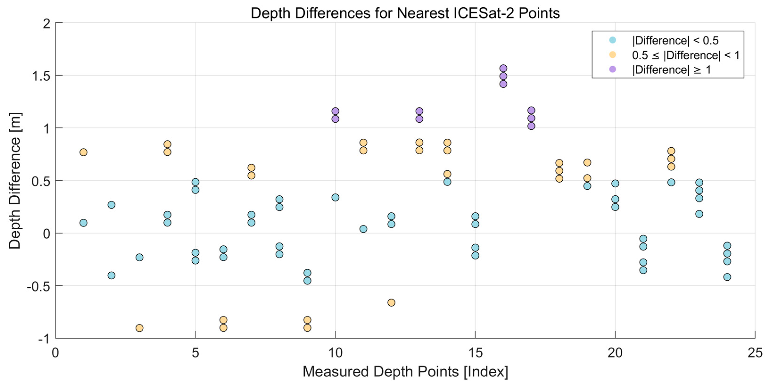
3.1. ICESat-2 Bathymetric Photon Extraction Results and Bathymetric Performance Evaluation

The ICESat-2 bathymetric photon data of Lingshui-Sanya Bay and Dongsha Islands were extracted using the fully automated bathymetric photon extraction algorithm constructed in this study (shown in Figure 6). Among them, 11,144 ICESat-2 bathymetry points were extracted from Lingshui-Sanya Bay and 10,581 bathymetry points were extracted from Dongsha Islands. In order to evaluate the accuracy of the ICESat-2 bathymetry data, we coordinate-matched the measured bathymetry data of Lingshui-Sanya Bay with the ICESat-2 bathymetry data. During the matching process, the K Nearest Neighbour (KNN) algorithm was used to search for the five nearest ICESat-2 bathymetry points around each measured point. The average distance to the five nearest ICESat-2 points from each measured point was calculated to be 38.88 m. Using this method, we obtained a total of 120 data pairs and calculated the depth difference of each pair. In order to show the data differences more intuitively, different colors were used to classify the data points according to the absolute value of the depth differences, and a difference distribution map (shown in Figure 7) was drawn to visualize the error distribution between the measured bathymetry and the ICESat-2 bathymetry. The statistical analysis results are shown in

Table 3. Comparison of ICESat-2 bathymetry data with in situ measurements.

MeasuredPointIndex	MeanDepthDiff (m)	VarDepthDiff (m)	MSE (m)	RMSE (m)
1	0.50	0.14	0.36	0.60
2	0.00	0.14	0.11	0.33
3	−0.50	0.14	0.36	0.60
4	0.55	0.14	0.41	0.64
5	0.19	0.14	0.15	0.39
6	−0.45	0.14	0.32	0.57
7	0.40	0.06	0.20	0.45
8	0.10	0.06	0.06	0.24
9	−0.60	0.06	0.41	0.64
10	0.98	0.13	1.06	1.03
11	0.68	0.13	0.57	0.75
12	−0.02	0.13	0.10	0.32
13	0.94	0.03	0.90	0.95
14	0.64	0.03	0.43	0.65
15	−0.06	0.03	0.03	0.17
16	1.49	0.00	2.23	1.49
17	1.09	0.00	1.19	1.09
18	0.59	0.00	0.35	0.59
19	0.52	0.01	0.28	0.53
20	0.32	0.01	0.11	0.33
21	−0.22	0.02	0.06	0.24
22	0.62	0.02	0.39	0.63
23	0.32	0.02	0.11	0.34
24	−0.28	0.02	0.09	0.31
ALL	0.32	0.33	0.43	0.65

, where MeanDepthDiff represents the mean depth difference and VarDepthDiff represents the variance of depth differences. Overall, the ICESat-2 bathymetry data are slightly higher compared to the measured data, and the fluctuation of the bathymetry difference is small, the error is more stable, and all of them are within the acceptable range. This indicates that ICESat-2 data can obtain high-precision shallow water bathymetry data, which has good potential for bathymetric applications.

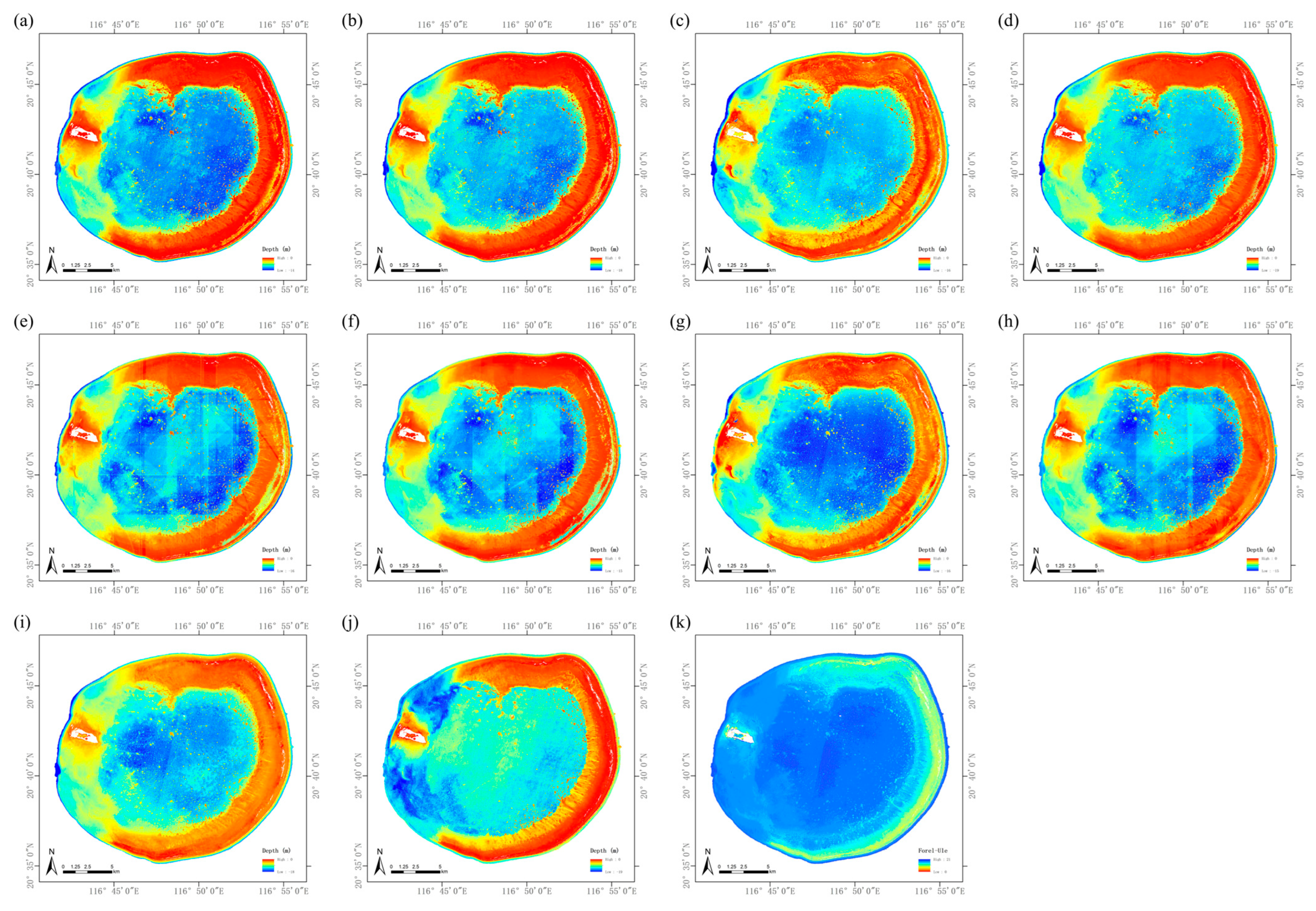
3.2. Bathymetric Inversion Based on Sentinel-2 Data

Through the preprocessing of Sentinel-2 imagery over the Dongsha Islands (Figure 1), we extracted the spectral characteristics of the region and performed data consistency processing, ultimately obtaining 9562 ICESat-2 bathymetry points. Using the computed FUI (shown in Figure 8k), we extracted the corresponding FUI values for the ICESat-2 bathymetry points and calculated the spatial information for each bathymetry point. Based on these data, we constructed a comprehensive information dataset and used it for model training. The trained model was then applied to perform bathymetry inversion for the Dongsha Islands (Figure 8). The inversion results from all machine learning models exhibited similar overall trends and were consistent with previous bathymetry inversion results for this region [43,69]. Therefore, our automated script for extracting ICESat-2 bathymetry points demonstrates good feasibility in shallow, clear-water areas, providing effective support for rapid bathymetric inversion.

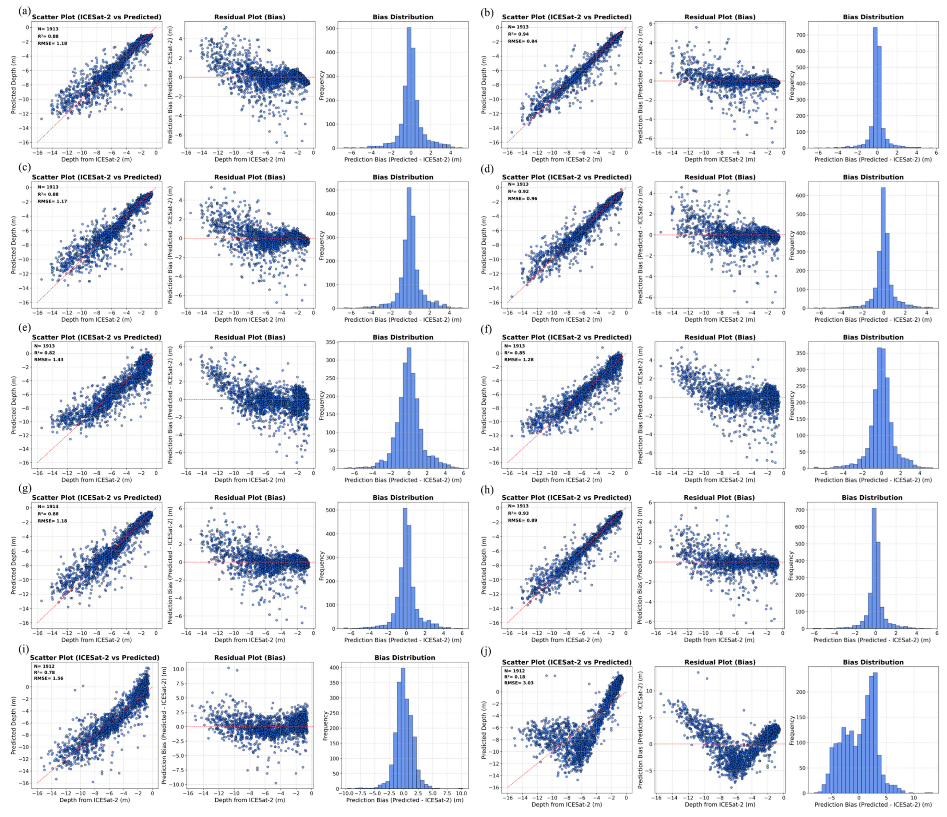
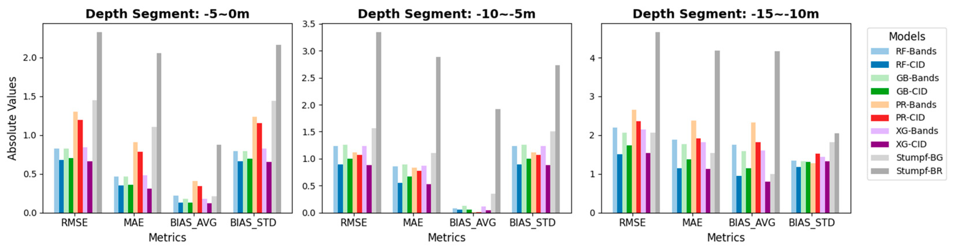
3.3. Evaluation of Model Accuracy

The trained models were evaluated on a 20% test set to assess their generalization. Scatter plots comparing predicted water depth with ICESat-2 depth values were generated to visually demonstrate the model’s prediction performance (as shown in Figure 9). Additionally, the R² and RMSE for each model were calculated on the test set to quantify the correlation between the predicted and true values, providing further validation of the model’s performance. The results indicate that the bathymetric inversion models using integrated features significantly improved R² and reduced RMSE compared to models with single features. When only spectral information was used as the input feature, the prediction performance of Random Forest, Gradient Boosting, and XGBoost models was similar. However, after incorporating water color information and spatial data, the Random Forest model performed the best, achieving an R² of 0.94 and an RMSE of 0.84 m.

4. Discussion

4.1. The Rationality of Feature Selection

In this study, we selected spectral information, spatial data (including normalized X and Y coordinates, as well as polar coordinates), and water color information (Forel-Ule Index, FUI) as model features. Spectral information is the core variable for bathymetric inversion, as water depth directly influences the absorption and scattering properties of light within the water column. Despite minimal changes in water quality within the study area, FUI, as a proxy for water color, provides complementary optical features. In clear waters, FUI assists in capturing subtle optical characteristics of the water, thereby enhancing the model’s ability to detect depth-related variations. The inclusion of spatial information, particularly normalized X and Y coordinates and polar coordinates, effectively captures spatial patterns in bathymetric distribution. The use of polar coordinates simplifies spatial calculations and improves the model’s ability to learn depth variations. By integrating these features, the model comprehensively accounts for optical, spatial, and water-related characteristics, ultimately improving the accuracy of bathymetric inversion and enhancing model performance in clear water environments.

4.2. Model Evaluation

To further evaluate the predictive performance of the models, residual and bias distribution plots were generated (as shown in Figure 9). Statistical analysis was performed for three depth ranges: from −5 m to 0 m, from −10 m to −5 m, and from −15 m to −10 m. The root mean square error (RMSE), mean absolute error (MAE), bias average (BIAS_AVG), and bias standard deviation (BIAS_STD) for each depth range were calculated (as shown in

Table 4. Statistics for different depth bands for different models.

Model	Segment	N	RMSE	MAE	BIAS_AVG	BIAS_STD
RF-Bands	−5~0 m	1006	0.82	0.46	−0.22	0.79
	−10~−5 m	727	1.23	0.86	−0.08	1.23
	−15~−10 m	179	2.20	1.88	1.75	1.34
GB-Bands	−5~0 m	1006	0.82	0.46	−0.18	0.79
	−10~−5 m	727	1.26	0.89	−0.12	1.26
	−15~−10 m	179	2.07	1.77	1.58	1.33
PR-Bands	−5~0 m	1006	1.30	0.91	−0.41	1.23
	−10~−5 m	727	1.12	0.83	−0.01	1.12
	−15~−10 m	179	2.65	2.37	2.32	1.28
XG-Bands	−5~0 m	1006	0.84	0.48	−0.18	0.82
	−10~−5 m	727	1.23	0.87	−0.11	1.23
	−15~−10 m	179	2.15	1.81	1.60	1.43
RF-CID	−5~0 m	1006	0.68	0.35	−0.13	0.66
	−10~−5 m	727	0.89	0.55	−0.05	0.89
	−15~−10 m	179	1.51	1.15	0.94	1.18
GB-CID	−5~0 m	1006	0.70	0.36	−0.13	0.69
	−10~−5 m	727	1.00	0.67	−0.05	1.00
	−15~−10 m	179	1.74	1.37	1.15	1.31
PR-CID	−5~0 m	1006	1.19	0.78	−0.34	1.15
	−10~−5 m	727	1.07	0.77	−0.01	1.07
	−15~−10 m	179	2.36	1.91	1.81	1.52
XG-CID	−5~0 m	1006	0.66	0.31	−0.12	0.65
	−10~−5 m	727	0.88	0.53	−0.04	0.88
	−15~−10 m	179	1.54	1.12	0.79	1.32
Stumpf-BG	−5~0 m	998	1.45	1.10	0.21	1.44
	−10~−5 m	737	1.56	1.10	−0.35	1.51
	−15~−10 m	175	2.06	1.54	0.99	1.81
Stumpf-BR	−5~0 m	998	2.32	2.05	0.87	2.16
	−10~−5 m	737	3.34	2.89	−1.92	2.73
	−15~−10 m	175	4.65	4.18	4.17	2.05

). Additionally, bar charts of the performance evaluation metrics for each model across different depth ranges were plotted (as shown in Figure 10) to provide a comprehensive comparison of model performance at various depth intervals. RMSE and MAE reflect the predictive accuracy of the models, with lower values indicating smaller prediction errors within the depth ranges. BIAS_AVG and BIAS_STD reveal the bias in model predictions, with a lower BIAS_AVG indicating predictions closer to the true water depths and a smaller BIAS_STD suggesting higher stability in the model’s performance across different depth ranges.

The analysis indicates that incorporating comprehensive information as input features improves model accuracy across all depth intervals. In the range from −15 m to −10 m, prediction errors were significantly reduced, suggesting that the inclusion of comprehensive information enhances the accuracy of predictions for the deeper segments of the shallow water zone (from −15 m to −10 m). The XGBoost model with Comprehensive Information (XG-CID) as input features performed best across all depth intervals, especially in the range from −10 m to 0 m, where both RMSE and MAE remained low. The Random Forest model with Comprehensive Information (RF-CID) inputs followed closely, demonstrating stable performance across all depth intervals, particularly maintaining strong predictive capability in the range from −15 m to −10 m.

However, in the range from −15 m to −10 m, all models exhibited systematic positive bias, with prediction errors generally exceeding 1 m. This bias is likely related to the sparse data in this depth range. The ICESat-2 data in this region is relatively sparse, which limits the model’s ability to accurately capture the complex variation in water depth, leading to an overestimation of the water depth and resulting in positive bias.

Furthermore, to gain deeper insights into the contribution of each feature to the model’s predictions, we employed SHAP (Shapley Additive Explanations) plots to analyze the impact of each feature on the model’s outputs across different depth intervals. SHAP values were calculated for each feature, highlighting their importance in the model’s predictions for various depth ranges (Figure 11). The results indicate that spectral information contributed the most to the model’s depth predictions. Despite the relatively minor changes in water quality, the Forel-Ule Index (FUI), which represents water color, played a significant role in capturing the optical properties of the water. Additionally, spatial information also contributed to the model’s predictions. Through these analyses, we gained a clearer understanding of the model’s behavior, which provides a basis for further optimization.

4.3. Limitations and Directions for Improvement

Due to practical limitations, the in situ water depth data in Lingshui-Sanya Bay in this study reached a maximum depth of only 2 m. This depth restriction hindered a more in-depth analysis of the script’s ability to extract water depth photons in deeper waters, and as a result, a comprehensive validation of the script’s performance in deeper regions was not possible. However, the water depth inversion results obtained in this study align with previous experimental findings, indicating that the water depth photon extraction script can still effectively provide water depth information in shallow areas, thus offering a convenient tool for water depth inversion in shallow waters. It is worth noting that the portability of this script requires further investigation, particularly in regions with complex water characteristics, which will be a key focus for future research improvements. Further validation of ICESat-2’s performance in deeper waters will require more extensive and deeper in situ data.

Additionally, ICESat-2 faces certain technical limitations in ultra-shallow water areas, particularly in regions where the water depth is less than 2 m. Due to the similarity between the water surface and seabed echo signals, the lidar system struggles to effectively distinguish between the reflections from the water surface and the seabed, thereby affecting depth measurement accuracy. Consequently, the depth accuracy of ICESat-2 in this depth range is relatively low, limiting its application potential in ultra-shallow water zones.

Furthermore, the water depth photon data provided by ICESat-2 has relatively low spatial resolution, leading to data sparsity and uneven distribution in certain areas. The discontinuity of the data may impact the accuracy of water depth inversion, especially in regions where water body characteristics are complex or data are sparse. Future research could optimize the inversion process by improving data fusion methods, integrating additional high-resolution remote sensing data, and considering factors such as water depth spatial distribution and water body environments. This could enhance the accuracy and applicability of the model.

5. Conclusions

This study proposes a rapid bathymetric inversion method based on ICESat-2 and Sentinel-2 data, integrating spectral information, the Forel-Ule Index (FUI) as water color information, and spatial location data (normalized X and Y coordinates and polar coordinates). Building upon previous work, an automated script for extracting bathymetric photon data was developed, enabling users to easily obtain the required photon data by simply inputting the study area, photon orbit number, and date. This aims to facilitate the use of ICESat-2 data for a wider range of researchers.

Although the in situ water depth data in Sanya Bay only reached 2 m, the bathymetric inversion results for the Dongsha Islands in this study are consistent with previous research, validating the script’s effectiveness in shallow water regions. The performance evaluation of several machine learning models showed that the XGBoost model with comprehensive input features (XG-CID) performed best across all depth intervals, particularly in the range from −10 m to 0 m, where its prediction accuracy was especially notable. The Random Forest model with comprehensive input features (RF-CID) also demonstrated strong predictive capability in the range from −15 m to −10 m.

Through SHAP analysis, this study enhanced the model’s interpretability, visually illustrating the influence of each feature on the predictions across different depth intervals. Spectral information contributed the most to the depth predictions, while FUI and spatial data also played a significant role in improving prediction accuracy.

Future research will focus on improving the extraction of bathymetric photons, incorporating higher-resolution remote sensing data, and considering additional factors such as spatial distribution of water depths and water body environment to further enhance the accuracy and applicability of the model.

References

1. Wang, Y.; He, X.; Bai, Y.; Wang, D.; Zhu, Q.; Gong, F.; Yang, D.; Li, T. Satellite retrieval of benthic reflectance by combining lidar and passive high-resolution imagery: Case-I water. Remote Sens. Environ. 2022, 272, 112955. [Google Scholar] [CrossRef]
2. da Silveira, C.B.L.; Strenzel, G.M.R.; Maida, M.; Araujo, T.C.M.; Ferreira, B.P. Multiresolution Satellite-Derived Bathymetry in Shallow Coral Reefs: Improving Linear Algorithms with Geographical Analysis. J. Coast. Res. 2020, 36, 1247–1265. [Google Scholar] [CrossRef]
3. Kutser, T.; Hedley, J.; Giardino, C.; Roelfsema, C.; Brando, V.E. Remote sensing of shallow waters—A 50 year retrospective and future directions. Remote Sens. Environ. 2020, 240, 111619. [Google Scholar] [CrossRef]
4. Ma, S.; Tao, Z.; Yang, X.; Yu, Y.; Zhou, X.; Li, Z. Bathymetry Retrieval from Hyperspectral Remote Sensing Data in Optical-Shallow Water. Ieee Trans. Geosci. Remote Sens. 2014, 52, 1205–1212. [Google Scholar] [CrossRef]
5. Wang, Y.; Zhou, X.; Li, C.; Chen, Y.; Yang, L. Bathymetry Model Based on Spectral and Spatial Multifeatures of Remote Sensing Image. Ieee Geosci. Remote Sens. Lett. 2020, 17, 37–41. [Google Scholar] [CrossRef]
6. Kulbacki, A.; Lubczonek, J.; Zaniewicz, G. Acquisition of Bathymetry for Inland Shallow and Ultra-Shallow Water Bodies Using PlanetScope Satellite Imagery. Remote Sens. 2024, 16, 3165. [Google Scholar] [CrossRef]
7. Bannari, A.; Kadhem, G. MBES-CARIS Data Validation for Bathymetric Mapping of ShallowWater in the Kingdom of Bahrain on the Arabian Gulf. Remote Sens. 2017, 9, 385. [Google Scholar] [CrossRef]
8. Costa, B.M.; Battista, T.A.; Pittman, S.J. Comparative evaluation of airborne LiDAR and ship-based multibeam SoNAR bathymetry and intensity for mapping coral reef ecosystems. Remote Sens. Environ. 2009, 113, 1082–1100. [Google Scholar] [CrossRef]
9. Ji, X.; Ma, Y.; Zhang, J.; Xu, W.; Wang, Y. A Sub-Bottom Type Adaption-Based Empirical Approach for Coastal Bathymetry Mapping Using Multispectral Satellite Imagery. Remote Sens. 2023, 15, 3570. [Google Scholar] [CrossRef]
10. Ashphaq, M.; Srivastava, P.K.; Mitra, D. Review of near-shore satellite derived bathymetry: Classification and account of five decades of coastal bathymetry research. J. Ocean Eng. Sci. 2021, 6, 340–359. [Google Scholar] [CrossRef]
11. Xie, C.; Chen, P.; Zhang, S.; Huang, H. Nearshore Bathymetry from ICESat-2 LiDAR and Sentinel-2 Imagery Datasets Using Physics-Informed CNN. Remote Sens. 2024, 16, 511. [Google Scholar] [CrossRef]
12. Knudby, A.; Richardson, G. Incorporation of neighborhood information improves performance of SDB models. Remote Sens. Appl. -Soc. Environ. 2023, 32, 101033. [Google Scholar] [CrossRef]
13. He, C.L.; Jiang, Q.G.; Wang, P. An Improved Physics-Based Dual-Band Model for Satellite-Derived Bathymetry Using SuperDove Imagery. Remote Sens. 2024, 16, 3801. [Google Scholar] [CrossRef]
14. Klotz, A.N.; Almar, R.; Quenet, Y.; Bergsma, E.W.J.; Youssefi, D.; Artigues, S.; Rascle, N.; Sy, B.A.; Ndour, A. Nearshore satellite-derived bathymetry from a single-pass satellite video: Improvements from adaptive correlation window size and modulation transfer function. Remote Sens. Environ. 2024, 315, 114411. [Google Scholar] [CrossRef]
15. Richardson, G.; Foreman, N.; Knudby, A.; Wu, Y.L.; Lin, Y.W. Global deep learning model for delineation of optically shallow and optically deep water in Sentinel-2 imagery. Remote Sens. Environ. 2024, 311, 114302. [Google Scholar] [CrossRef]
16. Wu, Z.Q.; Zhao, Y.C.; Wu, S.L.; Chen, H.D.; Song, C.H.; Mao, Z.H.; Shen, W. Satellite-Derived Bathymetry Using a Fast Feature Cascade Learning Model in Turbid Coastal Waters. J. Remote Sens. 2024, 4. [Google Scholar] [CrossRef]
17. Dietrich, J.T. Bathymetric Structure-from-Motion: Extracting shallow stream bathymetry from multi-view stereo photogrammetry. Earth Surf. Process. Landf. 2017, 42, 355–364. [Google Scholar] [CrossRef]
18. Lubczonek, J.; Kazimierski, W.; Zaniewicz, G.; Lacka, M. Methodology for Combining Data Acquired by Unmanned Surface and Aerial Vehicles to Create Digital Bathymetric Models in Shallow and Ultra-Shallow Waters. Remote Sens. 2022, 14, 105. [Google Scholar] [CrossRef]
19. Hodúl, M.; Chénier, R.; Faucher, M.A.; Ahola, R.; Knudby, A.; Bird, S. Photogrammetric Bathymetry for the Canadian Arctic. Mar. Geod. 2020, 43, 23–43. [Google Scholar] [CrossRef]
20. Del Savio, A.A.; Torres, A.L.; Olivera, M.A.V.; Rojas, S.R.L.; Ibarra, G.T.U.; Neckel, A. Using UAVs and Photogrammetry in Bathymetric Surveys in Shallow Waters. Appl. Sci. 2023, 13, 3420. [Google Scholar] [CrossRef]
21. Bandini, F.; Sunding, T.P.; Linde, J.; Smith, O.; Jensen, I.K.; Köppl, C.J.; Butts, M.; Bauer-Gottwein, P. Unmanned Aerial System (UAS) observations of water surface elevation in a small stream: Comparison of radar altimetry, LIDAR and photogrammetry techniques. Remote Sens. Environ. 2020, 237, 111487. [Google Scholar] [CrossRef]
22. Ma, Y.; Xu, N.; Liu, Z.; Yang, B.; Yang, F.; Wang, X.H.; Li, S. Satellite-derived bathymetry using the ICESat-2 lidar and Sentinel-2 imagery datasets. Remote Sens. Environ. 2020, 250, 112047. [Google Scholar] [CrossRef]
23. Polcyn, F.C.; Rollin, R.A. Remote sensing techniques for the location and measurement of shallow-water features. Available online: https://deepblue.lib.umich.edu/handle/2027.42/7114 (accessed on 6 June 2024).
24. Polcyn, F.C.; Brown, W.L.; Sattinger, I.J. The Measurement of Water Depth by Remote Sensing Techniques. Available online: https://agris.fao.org/search/en/providers/122415/records/647368ca53aa8c89630d65ca (accessed on 6 June 2024).
25. Polcyn, F.C. Calculations of water depth from ERTS-MSS data. Available online: https://ntrs.nasa.gov/citations/19730019626 (accessed on 6 June 2024).
26. Lyzenga, D.R. Passive remote sensing techniques for mapping water depth and bottom features. Appl. Opt. 1978, 17, 379–383. [Google Scholar] [CrossRef]
27. Lyzenga, D.R. Remote sensing of bottom reflectance and water attenuation parameters in shallow water using aircraft and Landsat data. Int. J. Remote Sens. 1981, 2, 71–82. [Google Scholar] [CrossRef]
28. Lyzenga, D.R. Shallow-water bathymetry using combined lidar and passive multispectral scanner data. Int. J. Remote Sens. 1985, 6, 115–125. [Google Scholar] [CrossRef]
29. Lyzenga, D.R.; Malinas, N.P.; Tanis, F.J. Multispectral bathymetry using a simple physically based algorithm. IEEE Trans. Geosci. Remote Sens. 2006, 44, 2251–2259. [Google Scholar] [CrossRef]
30. Stumpf, R.P.; Holderied, K.; Sinclair, M. Determination of water depth with high-resolution satellite imagery over variable bottom types. Limnol. Oceanogr. 2003, 48. [Google Scholar] [CrossRef]
31. Pacheco, A.; Horta, J.; Loureiro, C.; Ferreira, Ó. Retrieval of nearshore bathymetry from Landsat 8 images: A tool for coastal monitoring in shallow waters. Remote Sens. Environ. 2015, 159, 102–116. [Google Scholar] [CrossRef]
32. Hedley, J.D.; Roelfsema, C.; Brando, V.; Giardino, C.; Kutser, T.; Phinn, S.; Mumby, P.J.; Barrilero, O.; Laporte, J.; Koetz, B. Coral reef applications of Sentinel-2: Coverage, characteristics, bathymetry and benthic mapping with comparison to Landsat 8. Remote Sens. Environ. 2018, 216, 598–614. [Google Scholar] [CrossRef]
33. Sandidge, J.; Holyer, R.J. Coastal bathymetry from hyperspectral observations of water radiance. Remote Sens. Environ. 1998, 65, 341–352. [Google Scholar] [CrossRef]
34. Manessa, M.D.M.; Kanno, A.; Sekine, M.; Haidar, M.; Yamamoto, K.; Imai, T.; Higuchi, T. Satellite-Derived Bathymetry Using Random Forest Algorithm and Worldview-2 Imagery. Geoplanning J. Geomat. Plan. 2016, 3, 117–126. [Google Scholar] [CrossRef]
35. Wang, L.; Liu, H.; Su, H.; Wang, J. Bathymetry retrieval from optical images with spatially distributed support vector machines. Giscience Remote Sens. 2019, 56, 323–337. [Google Scholar] [CrossRef]
36. Leng, Z.; Zhang, J.; Ma, Y.; Zhang, J. Underwater Topography Inversion in Liaodong Shoal Based on GRU Deep Learning Model. Remote. Sens. 2020, 12, 4068. [Google Scholar] [CrossRef]
37. Neumann, T.A.; Martino, A.J.; Markus, T.; Bae, S.; Bock, M.R.; Brenner, A.C.; Brunt, K.M.; Cavanaugh, J.; Fernandes, S.T.; Hancock, D.W.; et al. The Ice, Cloud, and Land Elevation Satellite-2 mission: A global geolocated photon product derived from the Advanced Topographic Laser Altimeter System. Remote Sens. Environ. 2019, 233, 111325. [Google Scholar] [CrossRef]
38. Markus, T.; Neumann, T.; Martino, A.; Abdalati, W.; Brunt, K.; Csatho, B.; Farrell, S.; Fricker, H.; Gardner, A.; Harding, D.; et al. The Ice, Cloud, and land Elevation Satellite-2 (ICESat-2): Science requirements, concept, and implementation. Remote Sens. Environ. 2017, 190, 260–273. [Google Scholar] [CrossRef]
39. Abdalati, W.; Zwally, H.J.; Bindschadler, R.; Csatho, B.; Farrell, S.L.; Fricker, H.A.; Harding, D.; Kwok, R.; Lefsky, M.; Markus, T.; et al. The ICESat-2 Laser Altimetry Mission. Proc. IEEE 2010, 98, 735–751. [Google Scholar] [CrossRef]
40. Smith, B.; Fricker, H.A.; Holschuh, N.; Gardner, A.S.; Adusumilli, S.; Brunt, K.M.; Csatho, B.; Harbeck, K.; Huth, A.; Neumann, T.; et al. Land ice height-retrieval algorithm for NASA’s ICESat-2 photon-counting laser altimeter. Remote Sens. Environ. 2019, 233, 111352. [Google Scholar] [CrossRef]
41. Wang, C.; Zhu, X.; Nie, S.; Xi, X.; Li, D.; Zheng, W.; Chen, S. Ground elevation accuracy verification of ICESat-2 data: A case study in Alaska, USA. Opt. Express 2019, 27, 38168–38179. [Google Scholar] [CrossRef]
42. Parrish, C.E.; Magruder, L.A.; Neuenschwander, A.L.; Forfinski-Sarkozi, N.; Alonzo, M.; Jasinski, M. Validation of ICESat-2 ATLAS Bathymetry and Analysis of ATLAS’s Bathymetric Mapping Performance. Remote Sens. 2019, 11, 1634. [Google Scholar] [CrossRef]
43. Hsu, H.-J.; Huang, C.-Y.; Jasinski, M.; Li, Y.; Gao, H.; Yamanokuchi, T.; Wang, C.-G.; Chang, T.-M.; Ren, H.; Kuo, C.-Y.; et al. A semi-empirical scheme for bathymetric mapping in shallow water by ICESat-2 and Sentinel-2: A case study in the South China Sea. Isprs J. Photogramm. Remote Sens. 2021, 178, 1–19. [Google Scholar] [CrossRef]
44. Chen, Y.; Le, Y.; Zhang, D.; Wang, Y.; Qiu, Z.; Wang, L. A photon-counting LiDAR bathymetric method based on adaptive variable ellipse filtering. Remote Sens. Environ. 2021, 256, 112326. [Google Scholar] [CrossRef]
45. Xie, C.; Chen, P.; Pan, D.; Zhong, C.; Zhang, Z. Improved Filtering of ICESat-2 Lidar Data for Nearshore Bathymetry Estimation Using Sentinel-2 Imagery. Remote Sens. 2021, 13, 4303. [Google Scholar] [CrossRef]
46. Peng, K.; Xie, H.; Xu, Q.; Huang, P.; Liu, Z. A Physics-Assisted Convolutional Neural Network for Bathymetric Mapping Using ICESat-2 and Sentinel-2 Data. IEEE Trans. Geosci. Remote Sens. 2022, 60, 3213248. [Google Scholar] [CrossRef]
47. Guo, X.; Jin, X.; Jin, S. Shallow Water Bathymetry Mapping from ICESat-2 and Sentinel-2 Based on BP Neural Network Model. Water 2022, 14, 3862. [Google Scholar] [CrossRef]
48. van der Woerd, H.J.; Wernand, M.R. Hue-Angle Product for Low to Medium Spatial Resolution Optical Satellite Sensors. Remote Sens. 2018, 10, 180. [Google Scholar] [CrossRef]
49. Fronkova, L.; Greenwood, N.; Martinez, R.; Graham, J.A.; Harrod, R.; Graves, C.A.; Devlin, M.J.; Petus, C. Can Forel-Ule Index Act as a Proxy of Water Quality in Temperate Waters? Application of Plume Mapping in Liverpool Bay, UK. Remote Sens. 2022, 14, 2375. [Google Scholar] [CrossRef]
50. Nie, Y.F.; Guo, J.T.; Sun, B.N.; Lv, X.Q. An evaluation of apparent color of seawater based on the in-situ and satellite-derived Forel-Ule color scale. Estuar. Coast. Shelf Sci. 2020, 246, 107032. [Google Scholar] [CrossRef]
51. Zhang, J.; Tian, J.; Li, X.; Wang, L.; Chen, B.; Gong, H.; Ni, R.; Zhou, B.; Yang, C. Leaf area index retrieval with ICESat-2 photon counting LiDAR. Int. J. Appl. Earth Obs. Geoinf. 2021, 103, 102488. [Google Scholar] [CrossRef]
52. Xing, Y.; Huang, J.; Gruen, A.; Qin, L. Assessing the Performance of ICESat-2/ATLAS Multi-Channel Photon Data for Estimating Ground Topography in Forested Terrain. Remote Sens. 2020, 12, 2084. [Google Scholar] [CrossRef]
53. Xiang, J.; Li, H.; Zhao, J.; Cai, X.; Li, P. Inland water level measurement from spaceborne laser altimetry: Validation and comparison of three missions over the Great Lakes and lower Mississippi River. J. Hydrol. 2021, 597, 126312. [Google Scholar] [CrossRef]
54. Magruder, L.; Neumann, T.; Kurtz, N. ICESat-2 Early Mission Synopsis and Observatory Performance. Earth Space Sci. 2021, 8, e2020EA001555. [Google Scholar] [CrossRef] [PubMed]
55. Liu, X.; Su, Y.; Hu, T.; Yang, Q.; Liu, B.; Deng, Y.; Tang, H.; Tang, Z.; Fang, J.; Guo, Q. Neural network guided interpolation for mapping canopy height of China’s forests by integrating GEDI and ICESat-2 data. Remote Sens. Environ. 2022, 269, 112844. [Google Scholar] [CrossRef]
56. Li, Y.; Gao, H.; Zhao, G.; Tseng, K.-H. A high-resolution bathymetry dataset for global reservoirs using multi-source satellite imagery and altimetry. Remote Sens. Environ. 2020, 244, 111831. [Google Scholar] [CrossRef]
57. Li, Y.; Gao, H.; Jasinski, M.F.; Zhang, S.; Stoll, J.D. Deriving High-Resolution Reservoir Bathymetry From ICESat-2 Prototype Photon-Counting Lidar and Landsat Imagery. Ieee Trans. Geosci. Remote Sens. 2019, 57, 7883–7893. [Google Scholar] [CrossRef]
58. Gwenzi, D.; Lefsky, M.A.; Suchdeo, V.P.; Harding, D.J. Prospects of the ICESat-2 laser altimetry mission for savanna ecosystem structural studies based on airborne simulation data. Isprs J. Photogramm. Remote Sens. 2016, 118, 68–82. [Google Scholar] [CrossRef]
59. Drusch, M.; Del Bello, U.; Carlier, S.; Colin, O.; Fernandez, V.; Gascon, F.; Hoersch, B.; Isola, C.; Laberinti, P.; Martimort, P.; et al. Sentinel-2: ESA’s Optical High-Resolution Mission for GMES Operational Services. Remote Sens. Environ. 2012, 120, 25–36. [Google Scholar] [CrossRef]
60. Markel, J. Shallow Water Bathymetry with ICESat-2 (Tutorial Led by Jonathan Markel at the 2023 ICESat-2 Hackweek). Available online: https://icesat-2-2023.hackweek.io/tutorials/bathymetry/bathymetry_tutorial.html (accessed on 24 February 2024).
61. Sutterley, T. Python Interpretation of the NASA Goddard Space Flight Center YAPC (“Yet Another Photon Classifier”) Algorithm. Available online: https://yapc.readthedocs.io/en/latest/ (accessed on 24 February 2024).
62. Xu, X.; Xu, S.; Jin, L.; Song, E. Characteristic analysis of Otsu threshold and its applications. Pattern Recognit. Lett. 2011, 32, 956–961. [Google Scholar] [CrossRef]
63. Bernardis, M.; Nardini, R.; Apicella, L.; Demarte, M.; Guideri, M.; Federici, B.; Quarati, A.; De Martino, M. Use of ICEsat-2 and Sentinel-2 Open Data for the Derivation of Bathymetry in Shallow Waters: Case Studies in Sardinia and in the Venice Lagoon. Remote Sens. 2023, 15, 2944. [Google Scholar] [CrossRef]
64. Harmel, T.; Chami, M.; Tormos, T.; Reynaud, N.; Danis, P.-A. Sunglint correction of the Multi-Spectral Instrument (MSI)-SENTINEL-2 imagery over inland and sea waters from SWIR bands. Remote Sens. Environ. 2018, 204, 308–321. [Google Scholar] [CrossRef]
65. He, C.L.; Jiang, Q.G.; Tao, G.F.; Zhang, Z.C. A Convolutional Neural Network with Spatial Location Integration for Nearshore Water Depth Inversion. Sensors 2023, 23, 8493. [Google Scholar] [CrossRef]
66. Breiman, L. Random forests. Mach. Learn. 2001, 45, 5–32. [Google Scholar] [CrossRef]
67. Friedman, J.H. Greedy function approximation: A gradient boosting machine. Ann. Stat. 2001, 29, 1189–1232. [Google Scholar] [CrossRef]
68. Chen, T.Q.; Guestrin, C.; Assoc Comp, M. XGBoost: A Scalable Tree Boosting System. In Proceedings of the 22nd ACM SIGKDD International Conference on Knowledge Discovery and Data Mining (KDD), San Francisco, CA, USA, 13–17 August 2016; pp. 785–794. [Google Scholar]
69. Xu, N.; Wang, L.; Zhang, H.-S.; Tang, S.; Mo, F.; Ma, X. Machine Learning Based Estimation of Coastal Bathymetry From ICESat-2 and Sentinel-2 Data. Ieee J. Sel. Top. Appl. Earth Obs. Remote Sens. 2024, 17, 1748–1755. [Google Scholar] [CrossRef]
Figure 1. Map of the study area for this study. (a) Location of the study area for this study. (b) Sentinel-2 image map of Dongsha Islands. (c) Sentinel-2 image map of Lingshui-Sanya Bay; the red dots are the actual measurement points of water depth.
Remotesensing 16 04603 g001
Figure 2. The technical flowchart of this study. The blue dashed box illustrates the key steps in the ICESat-2 bathymetric photon extraction process.
Remotesensing 16 04603 g002
Figure 3. Noise and land photons were filtered using the YAPC algorithm. The right panel shows a zoomed-in view of the rectangular area in the image. (a) Photon signal density confidence map based on the YAPC algorithm, with red areas indicating high-confidence regions. (b) Water signal estimation map, where the red dots represent valid photon signals from the water surface and below.
Remotesensing 16 04603 g003
Figure 4. Reference lines for filtering noise and land photons. (a) The Otsu threshold method is used to automatically determine the minimum threshold for valid photon signals, with the red vertical line representing the threshold line for valid photon signals. (b) The estimated water surface height is obtained based on the histogram statistics of valid photon signals along the track, with the vertical black line indicating the estimated water surface height.
Remotesensing 16 04603 g004
Figure 5. Water depth map after refraction correction. The gray points represent uncorrected photon data, while the black points indicate refraction-corrected photon data. The blue points denote estimated water surface photons, and the red line represents the estimated seafloor.
Remotesensing 16 04603 g005
Figure 6. Plot of ICESat-2 bathymetric photon extraction data results. (a) Lingshui-Sanya Bay. (b) Dongsha Islands.
Remotesensing 16 04603 g006
Figure 7. Difference distribution map showing the distribution of depth differences between the measured points and the nearest ICESat-2 bathymetry points. The X-axis represents the sequence number of the measured points.
Remotesensing 16 04603 g007
Figure 8. Plot of inversion results based on four models for Dongsha Islands, where ‘-Bands’ represents bathymetric images inverted using spectral characteristic information, and ‘-CID’ represents bathymetric images inverted using comprehensive information. (a) Random Forest-Bands. (b) Gradient Boosting-Bands. (c) Polynomial Regression-Bands. (d) XGBoost-Bands. (e) Random Forest-CID. (f) Gradient Boosting-CID. (g) Polynomial Regression-CID. (h) XGBoost-CID. (i) Stumpf-BG. (j) Stumpf-BR. (k) Forel-Ule Index.
Remotesensing 16 04603 g008
Figure 9. Scatter plots, residual plots, and deviation distributions of predicted bathymetry versus ICESat-2 bathymetry values. (a) Random Forest-Bands. (b) Gradient Boosting-Bands. (c) Polynomial Regression-Bands. (d) XGBoost-Bands. (e) Random Forest-CID. (f) Gradient Boosting-CID. (g) Polynomial Regression-CID. (h) XGBoost-CID. (i) Stumpf-BG. (j) Stumpf-BR.
Remotesensing 16 04603 g009
Figure 10. The bar charts of performance evaluation metrics for each model across different depth ranges.
Remotesensing 16 04603 g010
Figure 11. SHAP analysis of feature contributions across depth intervals. The leftmost plot in each group represents the overall analysis, covering feature contribution analysis across all depth intervals, while the remaining plots correspond to different depth intervals. (a) Random Forest-CID. (b) Gradient Boosting-CID. (c) XGBoost-CID.
Remotesensing 16 04603 g011