Trajectory PHD and CPHD Filters for the Pulse Doppler Radar

Abstract

Different from the standard probability hypothesis density (PHD) and cardinality probability hypothesis density (CPHD) filters, the trajectory PHD (TPHD) and trajectory CPHD (TCPHD) filters employ the sets of trajectories rather than the sets of the targets as the variables for multi-target filtering. The TPHD and TCPHD filters exploit the inherent potential of the standard PHD and CPHD filters to generate the target trajectory estimates from first principles. In this paper, we develop the TPHD and TCPHD filters for pulse Doppler radars (PD-TPHD and PD-TCPHD filters) to improve the multi-target tracking performance in the scenario with clutter. The Doppler radar can obtain the Doppler measurements of targets in addition to the position measurements of targets, and both measurements are integrated into the recursive filtering of PD-TPHD and PD-TCPHD. PD-TPHD and PD-TCPHD can propagate the best augmented Poisson and independent identically distributed multi-trajectory density approximation, respectively, through the Kullback–Leibler divergence minimization operation. Considering the low computational complexity of sequential filtering, Doppler measurements are sequentially applied to the Gaussian mixture implementation. Moreover, we perform the $L$-scan implementations of PD-TPHD and PD-TCPHD. Simulation results demonstrate the effectiveness and robustness of the proposed algorithms in the scenario with clutter.

1. Introduction

Multi-target tracking (MTT) refers to estimating an unknown, time-varying number of targets and their tracks based on sensor observations, with the core challenge lying in the uncertainty of data association (DA) [1]. In recent years, numerous researchers have proposed various algorithms based on DA to accomplish multi-target tracking, including joint probabilistic data association (JPDA) [2,3] and multiple hypothesis tracking (MHT) [4,5,6]. However, MTT algorithms based on DA encounter several issues, such as the problem of a non-deterministic polynomial (NP) and the inability to manage target birth, death, and other dynamic changes precisely.

MTT algorithms based on the random finite set (RFS) model the multi-target states and multi-target measurements as time-varying sets, with the fundamental theory being an elegant multi-target Bayesian filter [7]. This approach eliminates the requirement for the measurement-to-track association by recursively propagating the filtering density of multi-target states, thus enabling the simultaneous estimation of the number of targets and their states. Nevertheless, due to the combinatorial nature of multi-target density and the multiple integrals of the infinite-dimensional multi-target state space, the computational complexity of the optimal multi-target Bayesian filter based on RFS is exceedingly large to be realized. To address the problem, Mahler has proposed a variety of principled approximations of the optimal multi-target Bayesian filter and the corresponding closed-form solutions under different conditions, including probability hypothesis density (PHD) [8,9,10], cardinality PHD (CPHD) [11,12,13], multi-Bernoulli (MB) [14], and hybrid Poisson multi-Bernoulli [15] filters. However, these filters cannot be strictly considered multi-target trackers because the target states are not distinguished. In order to produce trajectory in a principled manner and obtain the accurate closed-form solution of the optimal multi-target filtering density, generalized labeled MB (GLMB), δ-GLMB, and labeled MB (LMB) filters have been proposed by utilizing the conjugacy of the GLMB family in [16,17,18]. Due to the limited computational resources, the implementation of δ-GLMB filters is nearly infeasible, leading to the development of the marginalized δ-GLMB (Mδ-GLMB) filter. This filter, matching the first-order moment distribution and cardinality distribution of δ-GLMB density [19], preserves practical developability while retaining essential features. To mitigate performance loss and excessive computational burden from double truncation, refs. [20,21] proposed a sing-step δ-GLMB filter. Additionally, a multi-scan version of the GLMB model has been studied [22], significantly enhancing tracking performance. The models described in these filters are built on the classical Gaussian hidden Markov models. In other words, the state of the target depends only on the states of the last time, and the associated measurement depends only on its current states. To relax the restriction of the independence property, Bayesian multi-object filtering for pairwise Markov chains has been proposed in [23], which is motivated by the Kalman filtering using pairwise Gaussian models [24]. Therefore, the generalized versions with pairwise Markov models of the mentioned filters have been studied [25,26,27,28,29]. Among all of the filters, PHD, and CPHD filters have been widely used in various fields due to their high real-time performance and scalability, such as vehicular network positioning [30], multi-robot collaboration [31,32], and sensor networks and distributed fusion [33,34,35,36].

To address the issue that approximate filters cannot provide trajectory information in a mathematically rigorous way, the trajectory PHD (TPHD) and trajectory CPHD (TCPHD) filters were first introduced in [37]. The derivation of TPHD and TCPHD filters was performed in [38], which provides a new derivation of PHD and CPHD filters. The best Poisson and IID cluster density approximation can be obtained by minimizing the Kullback–Leibler divergence (KLD) of filtering density. Subsequently, ref. [39] offered a complete derivation of the TPHD filter, and the TPHD and TCPHD filters have provided a comprehensive overview in [37]. Specifically, TPHD propagates a Poisson multi-trajectory density forward in time on the space of sets of trajectories, while TCPHD propagates an independent identically distributed (IID) multi-trajectory density forward in time on the space of sets of trajectories. Later on, a trajectory Poisson multi-Bernoulli filter was proposed in [40]. The algorithm propagates Poisson multi-Bernoulli density forward in time and is capable of performing a closed-form implementation for sets of trajectories with Poisson birth models. Furthermore, the Poisson multi-Bernoulli mixture filtering in [41] has been extended to manage the spawned targets effectively [42]. The algorithms based on the sets of trajectories perform joint processing with historical estimates, providing trajectory information for standard approximate filters from first principles.

In the MTT of Doppler radars, Doppler measurements can be acquired in addition to obtaining the measurements of slant range, azimuth, and elevation of the targets. In traditional multi-target tracking algorithms, the augmentation of Doppler measurements is related to the convergence speed of the trajectory initiation and the accuracy of the data association [43]. Considering the potential correlation between the Doppler measurements and other measurement errors, neglecting this correlation will result in the deterioration of filtering accuracy [44,45]. Therefore, several algorithms have been proposed to improve the target tracking performance [46,47,48]. The data association is related to these algorithms, resulting in high amounts of computation. In [49,50,51,52,53,54], the filters based on the framework of RFS utilize Doppler measurements to conduct multi-target tracking.

In this paper, we aim to develop the trajectory PHD and CPHD filters for Pulse Doppler radars (PD-TPHD and PD-TCPHD filters). Our main contributions can be summarized as follows.

(1)

We derive the recursive equations for PD-TPHD and PD-TCPHD filters. Due to the dimensionality expansion of measurement information, the update process of the TPHD and TCPHD filters is modified. Hence, we establish a new measurement model and rederive the updated formulas for TPHD and TCPHD. The KLD minimization is also required for PD-TPHD and PD-TCPHD filters so that they can propagate the best Poisson multi-trajectory density and IID multi-trajectory density forward, respectively, during the recursive filtering.

(2)

Gaussian sequential mixture implementations of PD-TPHD and PD-TCPHD are performed. In the implementations, we model the posterior PHD of trajectories in a Gaussian sequential mixture form. Since the Doppler measurements are incorporated into the TPHD and TCPHD filters as augmented information, the dimension expansion of measurements occurs, so the computational complexity increases inevitably. To address the issue as much as possible, the implementations of the update are divided into two parts. Firstly, we adopt the position measurements to deal with the Gaussian mixture components of the predicted PHD and cardinality. Later on, the Doppler measurements are utilized to update the components. Gaussian sequential mixture filtering is able to obtain a lower computational burden compared to joint filtering while maintaining performance. We hold the fact that the current target states generally have an impact on the trajectory state estimates for recent time steps so that the joint density is propagated in the recent period while the independent density is propagated before this period.

The rest of this paper is organized as follows. The background on the sets of trajectories is given in Section 2. In Section 3, we establish the model of measurement and derive the PD-TPHD and PD-TCPHD filters. The Gaussian sequential implementations of the PD-TPHD and PD-TCPHD filters are provided in Section 4. Simulation experiments are shown in Section 5. The conclusions of the paper follow in Section 6.

2. Background

In this section, we briefly review the background of MTT in the space of sets of trajectories. The relevant definitions of trajectory RFS are introduced in Section 2.1, and the equations for Bayesian recursive filtering are presented in Section 2.2. In Section 2.3, we introduce the TPHD and TCPHD filters. More details can be referred to in [37].

2.1. The Relevant Definitions

In general, a single trajectory contains a set of target states with a start time and a duration. A trajectory can be represented as a variable $X=\left(t,x^{1:i}\right)$ mathematically, where $t$ is the initial time step of the trajectory, $x^{1:i}=\left(x^1,x^2,\dots ,x^i\right), x^{1:i}\in {\mathbb{R}}^{i{n}_x}$ is a sequence of the target states at consecutive time steps with length $i$, $n_x$ is the dimension of the single target state. Suppose that there are $n$ trajectories up to time $k$, the set of trajectories can be defined as

$${\mathbf{X}}_k=\left\{X_1,X_2,\dots ,X_n\right\}\in \mathcal{F}\left(T_{\left(k\right)}\right)$$

(1)

where $\mathcal{F}\left(T_{\left(k\right)}\right)$ is the set of all finite subsets of $T_{\left(k\right)}$, $T_{\left(k\right)}={\uplus }_{\left(t,i\right)\in I\left(k\right)}\left\{t\right\}\times {\mathbb{R}}^{i{n}_x}$ is the space of a single trajectory, $I\left(k\right)=\left\{\left(t,i\right):0\le t\le k, 1\le i\le k-t+1\right\}.$ To make the expression clear, the single trajectory state is denoted by the uppercase letter, and the subscript represents the target number. The multi-trajectory state is denoted by the bold letter, and the subscript represents the time.

A single trajectory density is given as ${\pi }_k\left(X\right)$, and its integral on the space $T_{\left(k\right)}$ is denoted as

$$\int {\pi }_k\left(X\right)dX=\sum _{\left(t,i\right)\in I\left(k\right)}\int {\pi }_k\left(t,x^{1:i}\right)d{x}^{1:i}$$

(2)

All possible conditions of the single trajectory, including the initial time, length, and states of the target, are contained in the integral. As for the multi-trajectory density ${\pi }_k\left({\mathbf{X}}_k\right)$, the set integral of ${\pi }_k\left({\mathbf{X}}_k\right)$ on the space $\mathcal{F}\left(T_{\left(k\right)}\right)$ is given by

$$\int {\pi }_k\left({\mathbf{X}}_k\right)\delta {\mathbf{X}}_k=\sum _{n=0}^{\infty }{\displaystyle \frac{1}{n!}}\int {\pi }_k\left(\left\{X_1,\dots ,X_n\right\}\right)d(X_1,\cdots ,X_n)$$

(3)

The multi-trajectory density ${\pi }_k\left({\mathbf{X}}_k\right)$ describes the joint distribution of elements in the set ${\mathbf{X}}_k$, and the derivation of PHD is based on the set integral of ${\pi }_k\left({\mathbf{X}}_k\right)$. It should be noted that the definition of the set integral focuses on the set of trajectories, and the set integral of ${\pi }_k\left({\mathbf{X}}_k\right)$ exists and is finite.

Due to the multiple integrals of the infinite-dimensional multi-trajectory state space, the PHD of the multi-trajectory density ${\pi }_k\left({\mathbf{X}}_k\right)$, matching the first moment, is given as

$$D_k\left(X\right)=\int {\pi }_k\left(\left\{X\right\}\cup {\mathbf{X}}_k\right)\delta {\mathbf{X}}_k$$

(4)

Given a region $C\subseteq T_{\left(k\right)}$, the expected number of trajectories in it can be obtained by

$$\begin{array}{ll}{\widehat{N}}_C& ={\int }_{C\subseteq T_{\left(k\right)}}{D}_k\left(X\right)dX\\ & ={\displaystyle \sum _{\left(t,i\right)\in I\left(k\right)}}\int 1_C\left(t,x^{1:i}\right)D_k\left(t,x^{1:i}\right)d{x}^{1:i}\end{array}$$

(5)

where $1_C\left(t,x^{1:i}\right)$ is the generalized indicator function, which is defined as

$$1_C\left(X\right)\stackrel{\scriptscriptstyle\mathrm{def}}{=}\left\{\begin{array}{ll}1,& \mathrm{if} X\subseteq C\\ 0,& \mathrm{else}\end{array}\right.$$

(6)

In addition, the generalized Kronecker delta is denoted as

$${\delta }_B\left[A\right]=\left\{\begin{array}{ll}1,& \mathrm{if} A=B\\ 0,& \mathrm{else}.\end{array}\right.$$

(7)

where $A$ and $B$ are discrete variables, and the generalized Kronecker delta is different from $\delta$ in the function of the integral set. Given two real-valued functions $f$ and $g$, the function of the inner product $〈f,g〉$ of the continuous function is defined as

$$〈f,g〉\stackrel{\scriptscriptstyle\mathrm{def}}{=}\int f\left(x\right)g(x)dx$$

(8)

Given a finite set $\mathcal{Z}-$ of real numbers, the elementary symmetric function $e_j\left(·\right)$ of order $j$ is given by

$$e_j(\mathcal{Z}-)=\sum _{S\subseteq \mathcal{Z}-,\left|S\right|=j}\left(\prod _{\zeta \in S}\zeta \right)$$

(9)

2.2. Bayesian Filtering Recursion of Trajectory RFS

The posterior multi-trajectory density ${\pi }_k(·)$ at time $k$ is calculated via the prediction and update steps:

$${\pi }_{k|k-1}({\mathbf{X}}_k)=\int f\left({\mathbf{X}}_k|{\mathbf{X}}_{k-1}\right){\pi }_{k-1}\left({\mathbf{X}}_{k-1}\right)\delta {\mathbf{X}}_{k-1}$$

(10)

$${\pi }_k({\mathbf{X}}_k)={\displaystyle \frac{g_k\left({\mathit{Z}}_{\mathrm{k}}|\tau {(\mathbf{X}}_k)\right){\pi }_{k|k-1}\left({\mathbf{X}}_{\mathrm{k}}\right)}{\int g_k\left({\mathit{Z}}_{\mathrm{k}}|\tau {(\mathbf{X}}_k)\right){\pi }_{k|k-1}\left({\mathbf{X}}_k\right)\delta {\mathbf{X}}_k}}$$

(11)

where ${\mathbf{X}}_{k-1}$ is the set of the trajectories at time $k-1$, ${\mathit{Z}}_{\mathrm{k}}$ is the set of measurements at time $k$. ${\pi }_{k|k-1}(·)$ is the predicted density at time $k$, $f\left({\mathbf{X}}_k|{\mathbf{X}}_{k-1}\right)$ is the transition density, ${\pi }_{k|k-1}\left({\mathbf{X}}_k\right)$ is the posterior density at time $k-1$, $g_k\left({\mathit{Z}}_{\mathrm{k}}|\tau {(\mathbf{X}}_k)\right)$ is the density of measurements given the current RFS of the targets, $\tau {(\mathbf{X}}_k)$ is the current state of the sets of trajectories at time $k$.

2.3. TPHD and TCPHD Filters

2.3.1. TPHD Filters

TPHD filters propagate a Poisson multi-trajectory density on the prediction and update steps followed by a KLD minimization. A Poisson multi-trajectory density $p(·)$ can be expressed as

$$p\left({\mathbf{X}}_k\right)=e^{-{\lambda }_k}{\lambda }_k^n\prod _{i=1}^n\breve{p}\left(X_i\right)$$

(12)

where ${\lambda }_k$ is the expected number of trajectories, $\breve{p}(·)$ is the density of a single trajectory. The recursion at time $k$ is based on the following assumptions:

• Each target evolves independently to generate measurements with survival probability $p_s(·)$ and transition probability $f(·|x)$, and the new targets are born independently.
• The clutter RFS, which belongs to Poisson with density $c(·)$, is independent of the measurements of targets.
• The predicted multi-trajectory RFS governed by the predicted multi-trajectory density represents a Poisson RFS.

Given the posterior multi-trajectory density at time $k-1$ ${\pi }_{k-1}\left({\mathit{X}}_{k-1}|{\mathit{Z}}_{1:k-1}\right)$, the predicted PHD $D_{k|k-1} \left(X\right)$ at time $k$ is

$$D_{k|k-1} \left(X\right)=D_{{\beta }_k}\left(X\right)+D_{s_k}\left(X\right)$$

(13)

where

$$D_{{\beta }_k}\left(t,x^{1:i}\right)=D_{\beta }\left(x^1\right){\delta }_k\left[t\right]$$

(14)

$$\begin{array}{ll}{D}_{s_k}& \left(X\right)\\ & =\left\{\begin{array}{cc}{p}_s\left(x^{i-1}\right)f\left(x^i|x^{i-1}\right)D_{k-1}\left(t,x^{1:i-1}\right),\hfill & t+i-1=k\\ \hfill 0,& \mathrm{else}\hfill \end{array}\right.\end{array}$$

(15)

is the PHD of the surviving trajectories, $D_{{\beta }_k}\left(X\right)$ is the PHD of the new trajectories at time $k$, $D_{k-1}\left(t,x^{1:i-1}\right)$ is the posterior PHD at time $k-1$. The updated PHD at time $k$ is

$$\begin{array}{ll}{D}_k \left(X\right)& ={\left(1-p_D\left(x^i\right)\right)D}_{k|k-1} \left(X\right)\\ & +p_D\left(x^i\right)D_{k|k-1} \left(X\right)\\ & \times {\displaystyle \sum _{z\in {\mathit{Z}}_k}}{\displaystyle \frac{g_k\left(z|x^i\right)}{{\lambda }_c\breve{c}\left(z\right)+⟨p_D{\left(·\right)g}_k\left(z|·\right),D_{k|k-1}^{\tau }\left(·\right)⟩}}\end{array}$$

(16)

where

$$D_{k|k-1}^{\tau }\left(y\right)=\sum _{t=1}^k\int D_{k\mid k-1}\left(t,x^{1:k-t},y\right)d{x}^{1:k-t}$$

(17)

denotes the PHD of the targets at time $k$, $p_D\left(x\right)$ is the detection probability, ${\lambda }_c$ is the rate of clutter, and $\breve{c}\left(z\right)$ is the spatial distribution of clutter in the surveillance region.

2.3.2. TCPHD Filters

TCPHD filters propagate an IID multi-trajectory density on the prediction and update steps, which are followed by a KLD minimization. An IID multi-trajectory density can be expressed as

$$p\left({\mathbf{X}}_k\right)={\rho }_k\left(n\right)n!\prod _{i=1}^n\breve{p}\left(X_i\right)$$

(18)

where $\breve{p}(·)$ is the density of a single trajectory, ${\rho }_k\left(n\right)$ is the density of the cardinality distribution. The recursion at time $k$ is based on the following assumptions:

• Each target evolves independently to generate measurements with survival probability $p_s$ and transition probability $f(·|x)$, and the new targets are born independently.
• The clutter RFS, which belongs to the IID cluster with density $c(·)$, is independent of the measurements of targets.
• The predicted multi-trajectory RFS governed by the predicted multi-trajectory density represents an IID cluster RFS.

Given the posterior multi-trajectory density at time $k-1$ ${\pi }_{k-1}\left({\mathit{X}}_{k-1}|{\mathit{Z}}_{1:k-1}\right)$, the predicted PHD $D_{k|k-1} \left(X\right)$ and cardinality distribution ${\rho }_{k|k-1}\left(n\right)$ at time $k$ are

$$D_{k|k-1} \left(X\right)=D_{{\beta }_k}\left(X\right)+D_{s_k}\left(X\right)$$

(19)

$$\begin{array}{ll}{\rho }_{k|k-1}\left(n\right)=& {\displaystyle \sum _{j=0}^n}{\rho }_{{\beta }_k}\left(n-j\right){\displaystyle \sum _{m=j}^{\infty }}{C}_m^j{\rho }_{k-1}\left(m\right)\\ & \times {\displaystyle \frac{{⟨p_s\left(·\right),D_{k-1}^{\tau }\left(·\right)⟩}^j{⟨1-p_s\left(·\right),D_{k-1}^{\tau }\left(·\right)⟩}^{m-j}}{⟨1,D_{k-1}^{\tau }\left(·\right)⟩}}\end{array}$$

(20)

where $D_{k-1}^{\tau }\left(·\right)$ denotes the PHD of the targets at time $k-1$, ${\rho }_{k-1}\left(·\right)$ denotes the posterior cardinality distribution at time $k-1$, ${\rho }_{{\beta }_k}\left(·\right)$ denotes the cardinality distribution of the new targets. The updated PHD $D_k \left(X\right)$ and the cardinality distribution ${\rho }_k\left(n\right)$ at time $k$ are

$${\rho }_k\left(n\right)={\displaystyle \frac{{\mathsf{{\rm Y}}}^0\left[D_{k|k-1}^{\tau },{\mathit{Z}}_k\right]\left(n\right){\rho }_{k|k-1}\left(n\right)}{⟨{\mathsf{{\rm Y}}}^0\left[D_{k|k-1}^{\tau },{\mathit{Z}}_k\right],{\rho }_{k|k-1}⟩}}$$

(21)

$$\begin{array}{ll}{D}_k \left(X\right)=& \left(1-p_D\left(x^i\right)\right)D_{k|k-1} \left(X\right)\\ & \times {\displaystyle \frac{⟨{\mathsf{{\rm Y}}}^1\left[D_{k|k-1}^{\tau },{\mathit{Z}}_k\right]{,\rho }_{k|k-1}⟩}{⟨{\mathsf{{\rm Y}}}^0\left[D_{k|k-1}^{\tau },{\mathit{Z}}_k\right]{,\rho }_{k|k-1}⟩}}\\ & +p_D\left(x^i\right)D_{k|k-1} \left(X\right)\\ & \times {\displaystyle \sum _{z\in {\mathit{Z}}_k}}{\displaystyle \frac{⟨{\mathsf{{\rm Y}}}^1[D_{k|k-1}^{\tau },{\mathit{Z}}_k\backslash \{z\left\}\right]{,\rho }_{k|k-1}⟩}{⟨{\mathsf{{\rm Y}}}^0\left[D_{k|k-1}^{\tau },{\mathit{Z}}_k\right]{,\rho }_{k|k-1}⟩}}{\displaystyle \frac{g\left(z|x^i\right)}{\breve{c}\left(z\right)}}\end{array}$$

(22)

$$\begin{array}{ll}{\mathsf{{\rm Y}}}^u\left[D_{k|k-1}^{\tau },{\mathit{Z}}_k\right]\left(n\right)=& {\displaystyle \sum _{j=0}^{\min \left(\left|{\mathit{Z}}_k\right|,n-u\right)}}\left(\left|{\mathit{Z}}_k\right|-j\right)!{\rho }_c\left(\left|{\mathit{Z}}_k\right|-j\right)\\ & \times {\displaystyle \frac{n!}{\left(n-j-u\right)!}}{e}_j\left(\mathsf{\Xi }\right(D_{k|k-1}^{\tau },{\mathit{Z}}_k\left)\right)\\ & \times {\displaystyle \frac{{⟨1-p_D\left(·\right),D_{k-1}^{\tau }\left(·\right)⟩}^{n-(j+u)}}{{⟨1,D_{k-1}^{\tau }⟩}^n}}\end{array}$$

$$\mathsf{\Xi }\left(D_{k|k-1}^{\tau },{\mathit{Z}}_k\right)=\left\{\int {\displaystyle \frac{g\left(z|x\right)}{\breve{c}\left(z\right)}}{p}_D\left(x\right)D_{k|k-1}^{\tau }\left(x\right)dx:z\in {\mathit{Z}}_k\right\}$$

(23)

The specific derivation of the above equations can be obtained in [37,39]. It should be noted that the TPHD and TCPHD filters mainly estimate the posterior multi-trajectory density of the alive trajectories, excluding the dead trajectories.

3. PD-TPHD and PD-TCPHD Filters

In this section, we focus on the derivation of PD-TPHD and PD-TCPHD. We establish the measurement model in Section 3.1. The updated steps of PD-TPHD and PD-TCPHD are provided in Section 3.2 and Section 3.3, respectively.

3.1. The Model of Measurements

The radar can obtain Doppler measurements of targets as augmented information, which is incorporated into the set of measurements to modify the filtering in the update step. Given the current set ${\mathbf{x}}_k=\{{\mathit{x}}_{k,1},{\mathit{x}}_{k,2},\dots ,{\mathit{x}}_{k,n}\}$, $N_k$ is the number of targets at time $k$, ${\mathit{x}}_{k,i}=\left[x_{k,i};{\dot{x}}_{k,i};y_{k,i};{\dot{y}}_{k,i}\right]$ is the state of the $i$th targets, including the position and velocity of the $i$th target. Suppose that the measurements of Doppler and location are disjoint; then the measurements of Doppler and location at time $k$ can be represented, respectively, as

$${\mathit{Z}}_d=\left\{z_{d,1},z_{d,2},\dots ,z_{d,M_k}\right\}=h_d\left({\mathbf{x}}_k\right)+{\mathit{n}}_d$$

(24)

$${\mathit{Z}}_l=\{z_{l,1},z_{l,2},\dots ,z_{l,M_k}\}=H_l{\mathbf{x}}_k+{\mathit{n}}_l$$

(25)

where

$$h_d\left({\mathit{x}}_{k,i}\right)={\displaystyle \frac{x_{k,i}{\dot{x}}_{k,i}+y_{k,i}{\dot{y}}_{k,i}}{\sqrt{x_{k,i}^2+y_{k,i}^2}}}$$

(26)

is the nonlinear function of Doppler measurement. ${\mathit{n}}_d$ is the corresponding Gaussian white noise matrix with zero mean and covariance ${\sigma }_d^2$, $M_k$ is the number of measurements, $z_{d,j}$is the $j$th measurement of the location, $H_l$ is the measurement matrix of the location, ${\mathit{n}}_l$ is the Gaussian white noise matrix with zero mean and covariance ${\mathit{R}}_c$, and $z_{l,j}$is the $j$th measurement of the Doppler.

In general, PD radar works with the staggered pulse repetition frequency model, which is higher than that of traditional radar. Due to its distinct properties over other radars, PD radar possesses excellent capabilities for clutter suppression and anti-jamming with no velocity ambiguity. Meanwhile, the working mode is beneficial in keeping the range measurements unambiguous. Therefore, the tracking accuracy will be effectively improved by adopting the PD radar.

It should be noted that we pay more attention to the derivation of the PD-TPHD and PD-TCPHD updates. As the Doppler measurements have an impact on the density of the measurements given the current RFS of targets, the PHD of the posterior and cardinality distribution are advanced to obtain a higher tracking performance. In this condition, the prediction step is in accordance with that of the TPHD and TCPHD filters.

3.2. Updated Step of the PD-TPHD Filter

We make the following assumptions while filtering at time $k$:

Assumption 1. 

Each target evolves independently and generates one measurement with density  $g_k\left(·|x\right)$.

Assumption 2. 

The clutter is independent of the measurements of the targets. The position of the clutter belongs to a Poisson RFS with density $p_{C,k}\left(·\right)$and clutter rate ${\lambda }_c$.

Assumption 3. 

The multi-trajectory predicted density and posterior density represent a Poisson RFS, respectively.

Since the prediction step is in accordance with that of TPHD filters, the prediction is omitted, and the details of the update are derived in this Section. On the basis of the above assumptions, the density of the measurement given the state at time $k$ is

$$\begin{array}{ll}g\left(\left[{\mathit{Z}}_l;{\mathit{Z}}_d\right]|{\mathbf{x}}_k\right)=& e^{-{\lambda }_c}\left[{\displaystyle \prod _{i=1}^n}(1-p_D\left({\mathit{x}}_{k,i}\right)\right]\\ & \times \left[{\displaystyle \prod _{j=1}^{M_k}}{\lambda }_c{p}_{C,k}\left(z_{l,j}\right)u_k\left(z_{d,j}\right)\right]\\ & \times {\displaystyle \sum _{\theta \in {\mathsf{\sigma }}_{n,M_k}}}{\displaystyle \prod _{i:{\theta }_i>0}}{\displaystyle \frac{p_D\left({\mathit{x}}_{k,i}\right)}{\left(1-p_D\left({\mathit{x}}_{k,i}\right)\right)}}\\ & \times {\displaystyle \frac{g_k\left(z_{d,{\theta }_i}|{\mathit{x}}_{k,i}\right)g_k\left(z_{l,{\theta }_i}|{\mathit{x}}_{k,i}\right)}{{\lambda }_c{p}_{C,k}\left(z_{l,{\theta }_i}\right)u_k\left(z_{d,{\theta }_i}\right)}}\end{array}$$

(27)

where ${\mathsf{\sigma }}_{n,M_k}$ represents the associations between the $n$ targets and $M_k$ measurements, $u_k\left(·\right)$ is the Doppler density of clutter, $i\in \left\{\mathrm{1,2},\dots ,n\right\}, j\in \{\mathrm{1,2},\dots ,M_k\}$, ${\theta }_i=j$ means target $i$ generates the measurement $j$ and ${\theta }_i=0$ means target $i$ has not been detected.

Proposition 1. 

Given the predicted PHD $D_{k|k-1} \left(X\right)$ at time $k$, the updated PHD is given by

$$D_k \left(X\right)=D_{k|k-1} \left(X\right)g\left(\left[{\mathit{Z}}_l;{\mathit{Z}}_d\right]|{\mathit{x}}_{k,i}\right)$$

(28)

where

$$\begin{array}{ll}g\left(\left[{\mathit{Z}}_l;{\mathit{Z}}_d\right]|{\mathit{x}}_{k,i}\right)=& 1-p_D\left({\mathit{x}}_k\right)+p_D\left({\mathit{x}}_k\right)\\ & \times {\displaystyle \sum _{\left[z_d,z_l\right]\in \left[{\mathit{Z}}_l;{\mathit{Z}}_d\right]}}{\displaystyle \frac{g_k\left(z_d|{\mathit{x}}_k\right)g_k\left(z_l|{\mathit{x}}_k\right)}{{\lambda }_c{p}_{C,k}\left(z_l\right)u_k\left(z_d\right)+D_{d,k}}}\end{array}$$

$$D_{d,k}=⟨p_D{\left(·\right)g}_k\left(z_d|·\right)g_k\left(z_l|·\right),D_{k|k-1}^{\tau }\left(·\right)⟩$$

(29)

Since only alive trajectories are considered, $D_k \left(X\right)\ne 0$ if $t+i-1=k$. To make the multi-trajectory density Poisson in the Bayesian recursion, a KLD minimization is required after the updated step. Additionally, the output of minimizing KLD is the best Poisson approximation to the filtering density. The detailed proof is in Appendix A. Compared to the TPHD filter, PD-TPHD not only considers the PHD of the alive-trajectory density but also augments the information with Doppler dimensions, which means that if we acquire a more accurate estimate of the Doppler, the accuracy of MTT will be improved.

3.3. Updated Step of the PD-TCPHD Filter

We make the additional assumptions while filtering at time $k$ on the basis of Assumption 1:

Assumption 4. 

The clutter is independent of the measurements of the targets. The position of the clutter belongs to an IID cluster RFS with density $p_{C,k}\left(·\right)$.

Assumption 5. 

The multi-trajectory predicted density and posterior density represent an IID cluster RFS, respectively.

Proposition 2. 

Given the predicted PHD $D_{k|k-1} \left(X\right)$ and cardinality distribution ${\rho }_{k|k-1}\left(n\right)$, the updated PHD and cardinality distribution are given by

$$\begin{gathered} \begin{array}{ll}{D}_k \left(X\right)=& \left(1-p_D\left(\mathit{x}\right)\right)D_{k|k-1} \left(X\right)\\ & \times {\displaystyle \frac{⟨{\mathsf{{\rm Y}}}^1\left[D_{k|k-1}^{\tau };{\mathit{Z}}_d;{\mathit{Z}}_l\right]{,\rho }_{k|k-1}⟩}{⟨{\mathsf{{\rm Y}}}^0\left[D_{k|k-1}^{\tau };{\mathit{Z}}_d;{\mathit{Z}}_l\right]{,\rho }_{k|k-1}⟩}}\\ & +p_D\left(\left(\mathit{x}\right)\right)D_{k|k-1} \left(X\right)\end{array} \\ \begin{array}{l}\times {\displaystyle \sum _{\left[z_d,z_l\right]\in \left[{\mathit{Z}}_l;{\mathit{Z}}_d\right]}}{\displaystyle \frac{⟨{\mathsf{{\rm Y}}}^1[D_{k|k-1}^{\tau };{\mathit{Z}}_k\backslash \{z_d;z_l\left\}\right]{,\rho }_{k|k-1}⟩}{⟨{\mathsf{{\rm Y}}}^0\left[D_{k|k-1}^{\tau };{\mathit{Z}}_k\right]{,\rho }_{k|k-1}⟩}}\\ \times {\displaystyle \frac{g_k\left(z_d|{\mathit{x}}_k\right)g_k\left(z_l|{\mathit{x}}_k\right)}{u_k\left(z_d\right)K_k\left(z_l\right)}}\end{array} \end{gathered}$$

(30)

$${\rho }_k\left(n\right)={\displaystyle \frac{{\mathsf{{\rm Y}}}^0\left[D_{k|k-1}^{\tau };{\mathit{Z}}_d;{\mathit{Z}}_l\right]\left(n\right){\rho }_{k|k-1}\left(n\right)}{⟨{\mathsf{{\rm Y}}}^0\left[D_{k|k-1}^{\tau };{\mathit{Z}}_d;{\mathit{Z}}_l]\right],{\rho }_{k|k-1}⟩}}$$

(31)

where

$$\begin{gathered} \begin{array}{ll}{\mathsf{{\rm Y}}}^u\left[D_{k|k-1}^{\tau },\left[{\mathit{Z}}_d;{\mathit{Z}}_l\right]\right]& \left(n\right)\\ & ={\displaystyle \sum _{j=0}^{\min \left(\left|{\mathit{Z}}_d\right|,n-u\right)}}\left(\left|{\mathit{Z}}_d\right|-j\right)!{\rho }_c\left(\left|{\mathit{Z}}_d\right|-j\right)\\ & \times {\displaystyle \frac{n!}{\left(n-j-u\right)!}}{e}_j\left(\mathsf{\Xi }\left(D_{k|k-1}^{\tau };{\mathit{Z}}_d;{\mathit{Z}}_l\right)\right)\\ & \times {\displaystyle \frac{{⟨1-p_D\left(·\right),D_{k-1}^{\tau }\left(·\right)⟩}^{n-\left(j+u\right)}}{{⟨1,D_{k-1}^{\tau }⟩}^n}}\end{array} \\ \mathsf{\Xi }\left(D_{k|k-1}^{\tau },[{\mathit{Z}}_d;{\mathit{Z}}_l]\right)= \\ \left\{\int {\displaystyle \frac{g\left(z_d|\mathit{x}\right)g\left(z_l|x\right)}{u_k\left(z_d\right)K_k\left(z_l\right)}}{p}_D\left(\mathit{x}\right)D_{k|k-1}^{\tau }\left(\mathit{x}\right)dx:\left[z_d,z_l\right]\in \left[{\mathit{Z}}_l;{\mathit{Z}}_d\right]\right\} \end{gathered}$$

(32)

${\mathrm{u}}_{\mathrm{k}}\left(·\right)$ is the intensity of Doppler clutter within a certain velocity range,  ${\mathrm{K}}_{\mathrm{k}}\left(·\right)$ denotes the intensity of the clutter of the location, $\mathsf{\Xi }\left({\mathrm{D}}_{\mathrm{k}|\mathrm{k}-1}^{\mathsf{\tau }},[{\mathbf{Z}}_{\mathrm{d}};{\mathbf{Z}}_{\mathrm{l}}]\right)$ are likelihood ratios of the weighted single detection likelihoods, ${\mathsf{{\rm Y}}}^0\left[{\mathrm{D}}_{\mathrm{k}|\mathrm{k}-1}^{\mathsf{\tau }};{\mathbf{Z}}_{\mathrm{d}};{\mathbf{Z}}_{\mathrm{l}}\right]\left(\mathrm{n}\right)$ is the likelihood of the measurements given $\mathrm{n}$ targets, $⟨{\mathsf{{\rm Y}}}^0\left[{\mathrm{D}}_{\mathrm{k}|\mathrm{k}-1}^{\mathsf{\tau }};{\mathbf{Z}}_{\mathrm{d}};{\mathbf{Z}}_{\mathrm{l}}]\right],{\mathsf{\rho }}_{\mathrm{k}|\mathrm{k}-1}⟩$ is a normalizing constant. Only alive trajectories are considered, ${\mathrm{D}}_{\mathrm{k}}\left(\mathrm{X}\right)\ne 0.$ if $\mathrm{t}+\mathrm{i}-1=\mathrm{k}$. PD-TCPHD propagates an IID cluster multi-trajectory density on the prediction and update steps, which follows a KLD minimization after the prediction and updated steps. The proof of the update step can be found in Appendix B. As the prediction of PD-TCPHD is identical to that of TCPHD, the prediction is omitted.

4. Gaussian Sequential Implementations

In this section, we provide the implementations of PD-TPHD and PD-TCPHD filters. The Gaussian sequential implementation of the PD-TPHD and PD-TCPHD filters are derived in Section 4.1 and Section 4.2, respectively. In Section 4.3, the $L$-scan approximation of the PD-TPHD and PD-TCPHD filters is provided. Finally, the estimations of the states of targets are performed in Section 4.4.

4.1. Gaussian Sequential Implementation of the PD-TPHD

In this section, we perform the closed-form sequential implementation of the PD-TPHD. The closed form of PD-TPHD requires the linear Gaussian mixture model in addition to the assumptions in Section 3.2. It can be seen that the linear Gaussian mixture model includes the standard linear Gaussian model for each target and other assumptions about birth, death, and spawning of targets. The detailed assumptions are given as follows:

Assumption 6. 

Each target follows the model of the linear Gaussian dynamic model, and the likelihood of measurements follows the linear Gaussian measuring model, which is given by

$$g\left({\mathit{x}}^{i+1}|{\mathit{x}}^i\right)=\mathcal{N}\left({\mathit{z}}_d;F{\mathit{x}}^i,Q\right)$$

(33)

$$g\left({\mathit{z}}_d|\mathit{x}\right)=\mathcal{N}\left({\mathit{z}}_d;H_l\mathit{x},{\mathit{R}}_c\right)$$

(34)

$$g\left({\mathit{z}}_l|\mathit{x}\right)=\mathcal{N}\left({\mathit{z}}_l;h_d\left(\mathit{x}\right),{\sigma }_d^2\right)$$

(35)

where $F$ is the transition matrix of the single target, $F\in {\mathbb{R}}^{n_x\times n_x}$, and $Q$ is the covariance matrix of the process noise of the single target, $Q\in {\mathbb{R}}^{n_x\times n_x}$. $\mathcal{N}\left(·;\mathit{m},\mathit{P}\right)$ indicates that the function follows the Gaussian distribution with mean $\mathit{m}$ and covariance $\mathit{P}$.

Assumption 7. 

The intensity of the newborn targets belongs to the Gaussian mixture form, which is given by

$$D_{{\beta }_k}\left(X\right)=\sum _{j=1}^{J_{\beta ,k}}{w}_{\beta ,k}^{\left(j\right)}\mathcal{N}\left(X;k,{\mathit{m}}_{\beta ,k}^{\left(j\right)},{\mathit{P}}_{\beta ,k}^{\left(j\right)}\right)$$

(36)

where $\mathcal{N}\left(\mathrm{X};\mathrm{k},{\mathbf{m}}_{\mathsf{\beta },\mathrm{k}}^{\left(\mathrm{j}\right)},{\mathbf{P}}_{\mathsf{\beta },\mathrm{k}}^{\left(\mathrm{j}\right)}\right)$ denotes the Gaussian density of a single trajectory with mean ${\mathbf{m}}_{\mathsf{\beta },\mathrm{k}}^{\left(\mathrm{j}\right)}$, covariance ${\mathbf{P}}_{\mathsf{\beta },\mathrm{k}}^{\left(\mathrm{j}\right)}$, and the assumed start time $\mathrm{k}$. If $\mathrm{t}=\mathrm{k}$, $\mathcal{N}\left(\mathrm{X};\mathrm{k},{\mathbf{m}}_{\mathsf{\beta },\mathrm{k}}^{\left(\mathrm{j}\right)},{\mathbf{P}}_{\mathsf{\beta },\mathrm{k}}^{\left(\mathrm{j}\right)}\right)=\mathcal{N}\left({\mathrm{x}}^{1:\mathrm{i}};{\mathbf{m}}_{\mathsf{\beta },\mathrm{k}}^{\left(\mathrm{j}\right)},{\mathbf{P}}_{\mathsf{\beta },\mathrm{k}}^{\left(\mathrm{j}\right)}\right)$, else $\mathcal{N}\left(\mathrm{X};\mathrm{k},{\mathbf{m}}_{\mathsf{\beta },\mathrm{k}}^{\left(\mathrm{j}\right)},{\mathbf{P}}_{\mathsf{\beta },\mathrm{k}}^{\left(\mathrm{j}\right)}\right)=0$. ${\mathrm{J}}_{\mathsf{\beta },\mathrm{k}}$ is the number of components, ${\mathrm{w}}_{\mathsf{\beta },\mathrm{k}}^{\left(\mathrm{j}\right)}$, ${\mathbf{m}}_{\mathsf{\beta },\mathrm{k}}^{\left(\mathrm{j}\right)}$, and ${\mathbf{P}}_{\mathsf{\beta },\mathrm{k}}^{\left(\mathrm{j}\right)},\mathrm{j}=\mathrm{1,2},\dots ,{\mathrm{J}}_{\mathsf{\beta },\mathrm{k}}$ are the weight, mean, and covariance of the $\mathrm{j}$th components of the new targets, respectively.

Based on the aforementioned assumptions on the recursive filtering of PD-TPHD, we perform the updated implementation in Proposition 3. The predicted implementation of PD-TPHD is omitted owing to the similarity to that of TPHD [39]. Given the additional enhancement of Doppler information, we can employ either joint or sequential filtering in the updated implementation with updated steps. Due to computational efficiency and analogous performance, the Gaussian sequential hybrid recursion can be selected, which utilizes the Doppler measurement to filter after updating the states of targets by using the location measurements. Finally, we calculate the weights by adopting both measurements.

Proposition 3. 

Given the predicted PHD at time $k$

$$D_{k|k-1} \left(X\right)=\sum _{j=1}^{J_{k|k-1}}{w}_{k|k-1}^{\left(j\right)}\mathcal{N}\left(X;t_{k|k-1}^{\left(j\right)},{\mathit{m}}_{k|k-1}^{\left(j\right)},{\mathit{P}}_{k|k-1}^{\left(j\right)}\right)$$

(37)

Then, the posterior PHD is given by

$$\begin{array}{ll}{D}_k \left(X\right)& =\left(1-p_D\right)D_{k|k-1} \left(X\right)\\ & +{\displaystyle \sum _{\left[z_d,z_l\right]\in \left[{\mathit{Z}}_l;{\mathit{Z}}_d\right]}}{D}_{k,v}\left(X;{\mathit{Z}}_l;{\mathit{Z}}_d\right)\end{array}$$

(38)

where

$$D_{k,v}\left(X;\mathit{z}\right)=\sum _{j=1}^{J_{k|k-1}}{w}_k^{\left(j\right)}\mathcal{N}\left(X;t_{k|k-1}^{\left(j\right)},{\mathit{m}}_{k|k}^{\left(j\right)},{\mathit{P}}_{k|k}^{\left(j\right)}\right)$$

(39)

$\mathcal{N}\left(\mathrm{X};{\mathrm{t}}_{\mathrm{k}|\mathrm{k}-1}^{\left(\mathrm{j}\right)},{\mathbf{m}}_{\mathrm{k}|\mathrm{k}-1}^{\left(\mathrm{j}\right)},{\mathbf{P}}_{\mathrm{k}|\mathrm{k}-1}^{\left(\mathrm{j}\right)}\right)$ denotes the Gaussian density of the $\mathrm{j}\mathrm{t}\mathrm{h}$ component with mean ${\mathbf{m}}_{\mathrm{k}|\mathrm{k}-1}^{\left(\mathrm{j}\right)}$, covariance ${\mathbf{P}}_{\mathrm{k}|\mathrm{k}-1}^{\left(\mathrm{j}\right)}$, and the assumed start time ${\mathrm{t}}_{\mathrm{k}|\mathrm{k}-1}^{\left(\mathrm{j}\right)}$. The concrete equations about ${\mathrm{w}}_{\mathrm{k}}^{\left(\mathrm{j}\right)}$, ${\mathrm{t}}_{\mathrm{k}|\mathrm{k}-1}^{\left(\mathrm{j}\right)}$, ${\mathbf{m}}_{\mathrm{k}|\mathrm{k}}^{\left(\mathrm{j}\right)},$ and ${\mathbf{P}}_{\mathrm{k}|\mathrm{k}}^{\left(\mathrm{j}\right)}$ can be found in the following proof.

Proof of Proposition 3. 

Firstly, the measurements of location are utilized to calculate the states of targets, which can be represented as

$${\mathit{m}}_{k|k}^{\left(j\right)}\left(z_l\right)={\mathit{m}}_{k|k-1}^{\left(j\right)}+{\mathit{G}}_l^{\left(\mathit{j}\right)}\left(z_l\right)\left(z_l-{\dot{\mathit{H}}}_l^{\left(j\right)}\left(z_l\right){\mathit{m}}_{k|k-1}^{\left(j\right)}\right)$$

(40)

$${\mathit{G}}_l^{\left(\mathit{j}\right)}={\mathit{P}}_{k|k-1}^{\left(j\right)}{\left({\dot{\mathit{H}}}_l^{\left(j\right)}\left(z_l\right)\right)}^{\mathrm{T}}{\left({\mathit{S}}_l^{\left(j\right)}\right)}^{-1}$$

(41)

$${\dot{\mathit{H}}}_l^{\left(j\right)}\left(z_l\right)=\left[0_{1,i_{l,k|k-1}^{\left(j\right)}-1},1\right]\otimes {\mathit{H}}_l^{\left(j\right)}\left(z_l\right)$$

(42)

$${\mathit{P}}_{k|k}^{\left(j\right)}\left(z_l\right)=\left[\mathit{I}-{\mathit{G}}_l^{\left(\mathit{j}\right)}{\dot{\mathit{H}}}_l^{\left(j\right)}\left(z_l\right)\right]{\mathit{P}}_{k|k-1}^{\left(j\right)}$$

(43)

$${\mathit{S}}_l^{\left(j\right)}={\dot{\mathit{H}}}_l^{\left(j\right)}{\mathit{P}}_{k|k-1}^{\left(j\right)}{\left({\dot{\mathit{H}}}_l^{\left(j\right)}\left(z_l\right)\right)}^{\mathrm{T}}+{\mathit{R}}_c$$

(44)

where ${\left(·\right)}^{\mathrm{T}}$, ${(·)}^{-1}$, and $\otimes$ denote the transpose operation, inverse operation, and Kronecker product, respectively. $i_{l,k|k-1}^{\left(j\right)}=\dim \left({\mathit{m}}_{k|k-1}^{\left(j\right)}\right)/n_x$. Then, we update the states of targets by the Doppler measurements sequentially, which is given by

$${\mathit{m}}_{k|k}^{\left(j\right)}={\mathit{m}}_{k|k}^{\left(j\right)}\left(z_l\right)+{\mathit{G}}_l^{\left(\mathit{j}\right)}\left(z_d\right)\left(z_d-{\widehat{z}}_{d,j}\right)$$

(45)

$${\widehat{z}}_{d,j}=h_d\left({\mathit{m}}_{k|k}^{\left(j\right)}\left(z_l\right)\right)$$

(46)

$${\mathit{G}}_d^{\left(j\right)}={\mathit{P}}_{k|k}^{\left(j\right)}\left(z_l\right){\left({\dot{\mathit{H}}}_d^{\left(j\right)}\left(z_d\right)\right)}^{\mathrm{T}}{\left({\mathit{S}}_d^{\left(j\right)}\right)}^{-1}$$

(47)

$${\dot{\mathit{H}}}_d^{\left(j\right)}\left(z_d\right)=\left[0_{1,i_{l,k|k-1}^{\left(j\right)}-1},1\right]\otimes {\mathit{H}}_d^{\left(j\right)}\left(z_d\right)$$

$${\mathit{S}}_d^{\left(j\right)}=\left({\dot{\mathit{H}}}_d^{\left(j\right)}\left(z_d\right)\right){\mathit{P}}_{k|k}^{\left(j\right)}\left(z_l\right){\left({\dot{\mathit{H}}}_d^{\left(j\right)}\left(z_d\right)\right)}^{\mathrm{T}}+{\sigma }_d^2$$

(48)

$${\mathit{P}}_{k|k}^{\left(j\right)}=\left[\mathit{I}-{\mathit{G}}_d^{\left(j\right)}{\dot{\mathit{H}}}_d^{\left(j\right)}\left(z_d\right)\right]{\mathit{P}}_{k|k}^{\left(j\right)}\left(z_l\right)$$

(49)

As ${\mathit{m}}_{k|k}^{\left(j\right)}\left(z_l\right)$ is rewritten as ${\mathit{m}}_{k|k}^{\left(j\right)}\left(z_l\right)=\left[x_{k|k}^{\left(j\right)}{\dot{x}}_{k|k}^{\left(j\right)}{y}_{k|k}^{\left(j\right)}{\dot{y}}_{k|k}^{\left(j\right)}\right]$, the Jacobian matrix of the Doppler measurements is calculated as

$${\mathit{H}}_d^{\left(j\right)}\left(\left(z_d\right)\right)=\nabla h_d\left(z_d\right)=\left[l_1{l}_2{l}_3{l}_4\right]$$

(50)

$$l_1={\displaystyle \frac{{\dot{x}}_{k|k}^{\left(j\right)}}{{\widehat{h}}_k^{\left(j\right)}}}-{\displaystyle \frac{{\widehat{z}}_{d,j}{x}_{k|k}^{\left(j\right)}}{{\left({\widehat{h}}_k^{\left(j\right)}\right)}^2}}$$

(51)

$$l_2={\displaystyle \frac{{\dot{y}}_{k|k}^{\left(j\right)}}{{\widehat{h}}_k^{\left(j\right)}}}-{\displaystyle \frac{{\widehat{z}}_{d,j}{y}_{k|k}^{\left(j\right)}}{{\left({\widehat{h}}_k^{\left(j\right)}\right)}^2}}$$

(52)

$$l_3={\displaystyle \frac{x_{k|k}^{\left(j\right)}}{{\widehat{h}}_k^{\left(j\right)}}}, l_4={\displaystyle \frac{y_{k|k}^{\left(j\right)}}{{\widehat{h}}_k^{\left(j\right)}}}$$

(53)

where ${\widehat{h}}_k^{\left(j\right)}={\left[{\left(x_{k|k}^{\left(j\right)} \right)}^2+{\left(y_{k|k}^{\left(j\right)}\right)}^2\right]}^{1/2}$. Subsequently, the weights of the Gaussian components can be represented as

$$\begin{array}{c}{w}_k^{\left(j\right)}={\displaystyle \frac{p_D{q}_k^{\left(j\right)}\left(z_d\right)q_k^{\left(j\right)}\left(z_l\right)}{K_k^l\left(z_l\right)K_k^d\left(z_d\right)+p_D\sum _{j=0}^{J_{k|k-1}}{w}_{k|k-1}^{\left(j\right)}{q}_k^{\left(j\right)}\left(z_d\right)q_k^{\left(j\right)}\left(z_l\right)}}\end{array}$$

(54)

where $K_k^l\left(z_l\right)={{\lambda }_{c}p}_{C,k}\left(z_l\right)$ is the intensity of the location measurements of clutter, $K_k^d\left(z_d\right)=u_k\left(z_d\right)$ is the intensity of the Doppler measurements of clutter. It can be obtained from (24) and (25) that the likelihood of measurements can be denoted as

$$q_k^{\left(j\right)}\left(z_d\right)=\mathcal{N}\left({\mathit{z}}_d;{\mathit{H}}_l^{\left(j\right)}{\mathit{m}}_{k|k-1}^{\left(j\right)},{\mathit{S}}_d^{\left(j\right)}\right)$$

(55)

$$q_k^{\left(j\right)}\left(z_l\right)=\mathcal{N}\left({\mathit{z}}_l;h_d\left({\mathit{m}}_{k|k}^{\left(j\right)}\left(z_l\right)\right),{\mathit{S}}_d^{\left(j\right)}\right)$$

(56)

 □

4.2. Gaussian Sequential Implementation of the PD-TCPHD

In this section, the closed-form sequential implementations of the PD-TCPHD, based on the assumptions in Section 3.3 and Section 4.1, are derived.

Proposition 4. 

If the predicted PHD $D_{k|k-1} \left(X\right)$ and cardinality distribution ${\rho }_{k|k-1}\left(n\right)$ are given as

$$\begin{array}{ll}{D}_{k|k-1}& \left(X\right)\\ & ={\displaystyle \sum _{j=1}^{J_{k|k-1}}}{w}_{k|k-1}^{\left(j\right)}\mathcal{N}\left(X;t_{k|k-1}^{\left(j\right)},{\mathit{m}}_{k|k-1}^{\left(j\right)},{\mathit{P}}_{k|k-1}^{\left(j\right)}\right)\end{array}$$

(57)

The posterior PHD $D_k \left(X\right)$, accompanied by a cardinality distribution ${\rho }_k\left(n\right)$, can be represented as

$${\rho }_k\left(n\right)={\displaystyle \frac{{\mathsf{{\rm Y}}}^0\left[w_{k|k-1};{\mathit{Z}}_l;{\mathit{Z}}_d\right]\left(n\right){\rho }_{k|k-1}\left(n\right)}{⟨{\mathsf{{\rm Y}}}^0\left[w_{k|k-1};{\mathit{Z}}_l;{\mathit{Z}}_d\right],{\rho }_{k|k-1}⟩}}$$

(58)

$$\begin{array}{ll}{D}_k \left(X\right)=& \left(1-p_D\right)D_{k|k-1} \left(X\right)\\ & \times {\displaystyle \frac{〈{\mathsf{{\rm Y}}}^1\left[w_{k|k-1};{\mathit{Z}}_l;{\mathit{Z}}_d\right]{\rho }_{k|k-1}〉}{⟨{\mathsf{{\rm Y}}}^0\left[w_{k|k-1};{\mathit{Z}}_l;{\mathit{Z}}_d\right],{\rho }_{k|k-1}⟩}}\\ & +{\displaystyle \sum _{\left[z_d,z_l\right]\in \left[{\mathit{Z}}_l;{\mathit{Z}}_d\right]}}{D}_{k,v}\left(X;{\mathit{Z}}_l;{\mathit{Z}}_d\right)\end{array}$$

(59)

where

$$D_{k,v}\left(X;\mathit{z}\right)=\sum _{j=1}^{J_{k|k-1}}{w}_k^{\left(j\right)}\mathcal{N}\left(X;t_{k|k-1}^{\left(j\right)},{\mathit{m}}_{k|k}^{\left(j\right)},{\mathit{P}}_{k|k}^{\left(j\right)}\right)$$

(60)

The concrete equations about $w_k^{\left(j\right)}$, $t_{k|k-1}^{\left(j\right)}$, ${\mathit{m}}_{k|k}^{\left(j\right)}$, and ${\mathit{P}}_{k|k}^{\left(j\right)}$ can be found in the following proof.

Proof of Proposition 4. 

As the implementation of the updated step is identical to that of PD-TPHD, the proof of this portion is omitted for simplicity. The mean and covariance of the single trajectory are displayed as (45) and 49), respectively. We derive the weights of the components as

$$\begin{array}{ll}{w}_k^{\left(j\right)}& ={\displaystyle \frac{p_D{w_{k|k-1}^{\left(j\right)}q}_k^{\left(j\right)}\left(z_d\right)q_k^{\left(j\right)}\left(z_l\right)〈1,K_k^l{K}_k^d〉}{K_k^l\left(z_l\right)K_k^d\left(z_d\right)}}\\ & \times {\displaystyle \frac{⟨{\mathsf{{\rm Y}}}^1[w_{k|k-1};{\mathit{Z}}_k\backslash \{z_d;z_l\left\}\right]{,\rho }_{k|k-1}⟩}{⟨{\mathsf{{\rm Y}}}^0\left[w_{k|k-1};{\mathit{Z}}_k\right]{,\rho }_{k|k-1}⟩}}\end{array}$$

(61)

where

$$\begin{array}{ll}{\mathsf{{\rm Y}}}^u\left[w,\left[{\mathit{Z}}_d;{\mathit{Z}}_l\right]\right]& \left(n\right)\\ & ={\displaystyle \sum _{j=0}^{\min \left(\left|{\mathit{Z}}_d\right|,n-u\right)}}\left(\left|{\mathit{Z}}_d\right|-j\right)!{\rho }_c\left(\left|{\mathit{Z}}_d\right|-j\right)\\ & \times {\displaystyle \frac{n!e_j\left(\mathsf{\Xi }\left(w;{\mathit{Z}}_d;{\mathit{Z}}_l\right)\right)}{\left(n-j-u\right)!}}\\ & \times {\displaystyle \frac{{⟨1-p_D\left(·\right)⟩}^{n-\left(j+u\right)}}{{⟨1,w⟩}^n}}\end{array}$$

(62)

$$\begin{array}{ll}\mathsf{\Xi }& \left(w,\left[{\mathit{Z}}_d;{\mathit{Z}}_l\right]\right)\\ & =\left\{{\displaystyle \frac{〈1,K_k^l{K}_k^d〉}{K_k^l\left(z_l\right)K_k^d\left(z_d\right)}}{p}_D{\mathit{w}}^{\mathrm{T}}{\mathit{q}}_k\left(z_d,z_l\right):\left[z_d,z_l\right]\in \left[{\mathit{Z}}_l;{\mathit{Z}}_d\right]\right\}\end{array}$$

(63)

$${\mathit{w}}_{\mathit{k}|\mathit{k}-1}={\left[w_{k|k-1}^{\left(1\right)},w_{k|k-1}^{\left(2\right)},\dots ,w_{k|k-1}^{\left(J_{k|k-1}\right)}\right]}^{\mathbf{T}}$$

(64)

$${\mathit{q}}_k\left(z_d,z_l\right)={\left[q_k^{\left(1\right)}\left(z_d\right)q_k^{\left(1\right)}\left(z_l\right),\dots ,q_k^{\left(J_{k|k-1}\right)}\left(z_d\right)q_k^{\left(J_{k|k-1}\right)}\left(z_l\right)\right]}^{\mathrm{T}}$$

(65)

The equations of $q_k^{\left(j\right)}\left(z_d\right)$ and $q_k^{\left(j\right)}\left(z_l\right)$ are provided in (55) and (56). It can be seen from (39) and (60) that the Gaussian sequential mixture implementation of PD-TPHD is confronted with the issues of an increasing number of components over time, which leads to a large computational burden. The number of Gaussian components at time $k$ is calculated as $J_k=\left(1+\left|{\mathit{Z}}_d\right|\right)\left[J_{k-1}\left(1+J_{\beta ,k}\right)+J_{\gamma ,k})\right]$. To control the increasing number of components, we utilize the pruning and absorption methods to manage the Gaussian components after the updated steps, as presented in Algorithm 1. The algorithm is similar to that in [37], except for the principle of absorption. The pruning step is achieved by discarding the components with weights below a certain threshold. Additionally, several adjacent components can be approximately represented by a single Gaussian component. □

Algorithm 1. The Steps of Pruning and Absorption.

Input: The Gaussian components after update steps ${\left\{w_k^{\left(j\right)},t_k^{\left(j\right)},{\mathit{m}}_{k|k}^{\left(j\right)}, {\mathit{P}}_{k|k}^{\left(j\right)}\right\}}_{j=1}^{J_k}$$, \mathrm{the} \mathrm{pruning} \mathrm{threshold} T$, $\mathrm{absorption} \mathrm{threshold} U$$, \mathrm{maximal} \mathrm{number} \mathrm{of} \mathrm{Gaussian} \mathrm{components} J_{\mathrm{m}\mathrm{a}\mathrm{x}}$.    Output: $\mathrm{The} \mathrm{Gaussian} \mathrm{components} \mathrm{after} \mathrm{pruning} \mathrm{and} \mathrm{absorption} {\left\{{\tilde{w}}_k^{\left(j\right)},{{\tilde{t}}_k^{\left(j\right)},\tilde{\mathit{m}}}_{k|k}^{\left(j\right)}, {\tilde{\mathit{P}}}_{k|k}^{\left(j\right)}\right\}}_{j=1}^r$.    −$\mathrm{set} r=0$ and $S=\left\{j=\mathrm{1,2},\dots ,J_k|w_k^{\left(j\right)}>T \right\}$    repeat    −$r\leftarrow r+1$.    -    $i=\underset{j\in S}{\arg }\max w_k^{\left(j\right)}$.    -$L=\left\{j\in S|{\left({\delta \mathit{m}}_{k|k}^{\left(j\right)}\right)}^{\mathrm{T}}{\left({\mathit{P}}_{k|k}^{\left(j\right)}\right)}^{-1}{\delta \mathit{m}}_{k|k}^{\left(j\right)}\right\}$, ${\delta \mathit{m}}_{k|k}^{\left(j\right)}= {\mathit{m}}_{k|k}^{\left(j\right)}-{\mathit{m}}_{k|k}^{\left(i\right)}$.    $- {\tilde{w}}_k^{\left(r\right)}=\sum _{j\in L}{w}_k^{\left(j\right)}$.    $- {\tilde{t}}_k^{\left(r\right)}=t_k^{\left(j\right)}.$    $- {\tilde{\mathit{m}}}_{k|k}^{\left(r\right)}={\displaystyle \frac{1}{{\tilde{w}}_k^{\left(r\right)}}}\sum _{j\in L}{w}_k^{\left(j\right)}{\mathit{m}}_{k|k}^{\left(j\right)}.$    $-{\tilde{\mathit{P}}}_{k|k}^{\left(r\right)}={\displaystyle \frac{1}{{\tilde{w}}_k^{\left(r\right)}}}\sum _{j\in L}{w}_k^{\left(j\right)}\left({\mathit{P}}_{k|k}^{\left(j\right)}+\left({\tilde{\mathit{m}}}_{k|k}^{\left(r\right)}-{\mathit{m}}_{k|k}^{\left(j\right)}\right){\left({\tilde{\mathit{m}}}_{k|k}^{\left(r\right)}-{\mathit{m}}_{k|k}^{\left(j\right)}\right)}^{\mathrm{T}}\right)$.    $- S\leftarrow S\backslash L$.    until $S=\varnothing$. -$\mathrm{If} r>J_{\mathrm{m}\mathrm{a}\mathrm{x}}$$, \mathrm{the} J_{\mathrm{m}\mathrm{a}\mathrm{x}}$ components with the largest weight are kept.

4.3. The L-Scan Approximations

In order to decrease the computational burden, the $L$-scan GMTPHD and GMTCPHD are firstly proposed in [37]. In this section, we aim to apply the $L$-scan approximations to the implementations of PD-TPHD and PD-TCPHD. The fundamental concept of the $L$-scan approximations is to propagate the joint density of the last $L$ time steps while maintaining the previous states in the original form. The parameters of the $L$-scan version, which contain the predicted mean and covariance of the targets, can be represented as

$${\mathit{m}}_{k|k-1}^{\left(j\right)}={\left[{\left({\mathit{m}}_{t_{k|k-1}^{\left(j\right)}:K-L-1}^{\left(j\right)}\right)}^{\mathrm{T}},{\left({\dot{\mathit{F}}}_{k-1}^{\left(j\right)}{\mathit{m}}_{k-L:k-1}^{\left(j\right)}\right)}^{\mathrm{T}}\right]}^{\mathrm{T}}$$

(66)

$${\dot{\mathit{F}}}^{\left(j\right)}=\left[0_{1,L-1},1\right]\otimes {\mathit{F}}^{\left(j\right)}$$

(67)

$${\mathit{P}}_{k|k-1}^{\left(j\right)}=\mathrm{d}\mathrm{i}\mathrm{a}\mathrm{g}({\mathit{P}}_{t_{k|k-1}^{\left(j\right)}}^{\left(j\right)},{\mathit{P}}_{t_{k|k-1}^{\left(j\right)}+1}^{\left(j\right)},..,{\mathit{P}}_{k-L+1:k}^{\left(j\right)})$$

(68)

where ${\mathit{m}}_{k-L:k-1}^{\left(j\right)}$ is the joint mean of the $L$ last time steps, ${\mathit{m}}_{k-L:k-1}^{\left(j\right)}\in {\mathbb{R}}^{L{n}_x}$, ${\mathit{P}}_{k-L+1:k}^{\left(j\right)}$ is the joint covariance matrix of the $L$ last time steps, ${\mathit{P}}_i^{\left(j\right)}, i=t_{k|k-1}^{\left(j\right)},{ t}_{k|k-1}^{\left(j\right)}+1,\dots ,k-L$ is the independent covariance matrix of the targets at time $i$. The above three equations are designed for $L>1$. When $L=1$, the $L$-scan version shares the same computations with the standard GMTPHD and GMTCPHD. The precision of joint density depends on the value of $L$, thereby establishing the relationship with the performance of MTT. Moreover, the specific value of $L$ is settled according to the practical requirement.

4.4. Estimation

In this section, we commonly discuss the estimators of the states and numbers of targets in the Gaussian sequential mixture PD-TPHD and PD-TCPHD. The number of trajectories at time $k$ for PD-TPHD can be given as

$${\widehat{N}}_k=\mathrm{r}\mathrm{o}\mathrm{u}\mathrm{n}\mathrm{d}\left(\sum _{j=1}^{J_k}{w}_k^{\left(j\right)}\right)$$

(69)

where $J_k$ is the number of components. Due to the augmentation of the cardinality distribution for the Gaussian sequential mixture PD-TCPHD, the number of trajectories is

$${\widehat{N}}_k=\arg \max {\rho }_k\left(·\right)$$

(70)

Based on the estimated numbers of trajectories and weights of PHD components, the estimated set of trajectories can be represented as

$$\left\{\left(t_1,{\widehat{m}}_{1,k}\right)),\dots ,\left(t_{{\widehat{N}}_k},{\widehat{m}}_{{\widehat{N}}_k,k}\right)\right\}$$

(71)

The ${\widehat{N}}_k$ highest weights of the components are selected to build the estimation of trajectories.

5. Simulation Experiments

In this section, several simulations are conducted to evaluate the performance of the algorithms. The targets move in the Cartesian plane with the size of $C=\left[0, 2000\right] \mathrm{m}\times \left[0, 2000\right] \mathrm{m}$ for 100 time steps. The target state is assumed as  $\mathit{x}={\left[p_x,{\dot{p}}_x,p_y, {\dot{p}}_y\right]}^{\mathrm{T}}$, which contains the position and velocity. The measurement matrix contains the location and Doppler measurements. The survival probability is constant, and $p_s=0.99$. The detection probability is constant, and $p_D=0.98$. ${\mathit{R}}_c={\sigma }_c^2{\mathit{I}}_2$, ${\mathit{I}}_2$ denotes the $2\times 2$ identity matrix, ${\sigma }_c^2=10 \mathrm{m}$, ${\sigma }_d^2=0.5 \mathrm{m}/\mathrm{s}$, $v_{\mathrm{m}\mathrm{a}\mathrm{x}}=35 \mathrm{m}/\mathrm{s}.$ The parameters of the dynamic process and measurements are

$$F=\left[\begin{array}{cc}{\mathit{I}}_2& ∆{\mathit{I}}_2\\ {\mathbf{0}}_2& {\mathit{I}}_2\end{array}\right]$$

$$Q={\sigma }_v^2\left[\begin{array}{cc}{∆}^4{\mathit{I}}_2/4& {∆}^3{\mathit{I}}_2/2\\ {∆}^3{\mathit{I}}_2/2& {∆}^2{\mathit{I}}_2\end{array}\right]$$

$$H_l=\left[\begin{array}{cccc}1& 0& 0& 0\\ 0& 1& 0& 0\end{array}\right]$$

where $∆=1 \mathrm{s}$, ${\sigma }_v^2=5 \mathrm{m}/\mathrm{s}$. In addition, the parameters of newborn targets are given as ${\mathit{m}}_{\beta }^{\left(1\right)}={\left[\mathrm{200,0},\mathrm{200,0}\right]}^{\mathrm{T}},$ ${\mathit{m}}_{\beta }^{\left(2\right)}={\left[\mathrm{500,0},\mathrm{700,0}\right]}^{\mathrm{T}},$ ${\mathit{m}}_{\beta }^{\left(3\right)}={\left[\mathrm{400,0},\mathrm{300,0}\right]}^{\mathrm{T}},$ $J_{\beta }=3,$ ${\mathit{w}}_{\beta }^{\left(j\right)}=0.1, {\mathit{P}}_{\beta }^{\left(j\right)}=\mathrm{d}\mathrm{i}\mathrm{a}\mathrm{g}\left(\left[\mathrm{225,100,225,100}\right]\right),j=\mathrm{1,2},3$. The parameters for state extractions are the following: the pruning threshold $T={10}^{-5}$, absorption threshold $U=4$, maximal number of Gaussian components $J_{\mathrm{m}\mathrm{a}\mathrm{x}}=100$, and the approximate truncated parameter of cardinality distribution is $N_{\mathrm{m}\mathrm{a}\mathrm{x}}=100$. Given the initial states, the newborn time and death time of the targets are in

Table 1. The initial states of targets.

	Birth Time/s	Death Time/s	Initial States
Target 1	1	80	${\left[\mathrm{205,10,202,12}\right]}^{\mathrm{T}}$
Target 2	10	80	${\left[502,-\mathrm{15,701},-4\right]}^{\mathrm{T}}$
Target 3	10	80	${\left[\mathrm{399,10,295,10}\right]}^{\mathrm{T}}$
Target 4	10	80	${\left[201,-\mathrm{3,207,12}\right]}^{\mathrm{T}}$
Target 5	20	100	${\left[\mathrm{505,3},695,-8\right]}^{\mathrm{T}}$
Target 6	20	100	${\left[405,-\mathrm{4,305,10}\right]}^{\mathrm{T}}$
Target 7	20	90	${\left[402,-\mathrm{10,301,2}\right]}^{\mathrm{T}}$

.

In order to evaluate the performance of the MTT, the trajectory metric (TM) is utilized [55] with Monte Carlo experiments, where $N_{\mathrm{m}\mathrm{c}}=1000$, $p=2, c=10, \gamma =1.$ The TM calculates the error between the true trajectories ${\mathbf{X}}_k$ and the corresponding estimated trajectories ${\tilde{\mathbf{X}}}_k$, which contain the errors for missed targets, false targets, localization, and track switches. The root mean square error (RMSE) of trajectories at time $k$ is written as

$$\mathrm{R}\mathrm{M}\mathrm{S}\mathrm{E}=\sqrt{\sum _{i=1}^{N_{\mathrm{m}\mathrm{c}}}{\displaystyle \frac{d^2\left({\mathbf{X}}_k,{\tilde{\mathbf{X}}}_{k,i}\right)}{k{N}_{\mathrm{m}\mathrm{c}}}}}$$

(72)

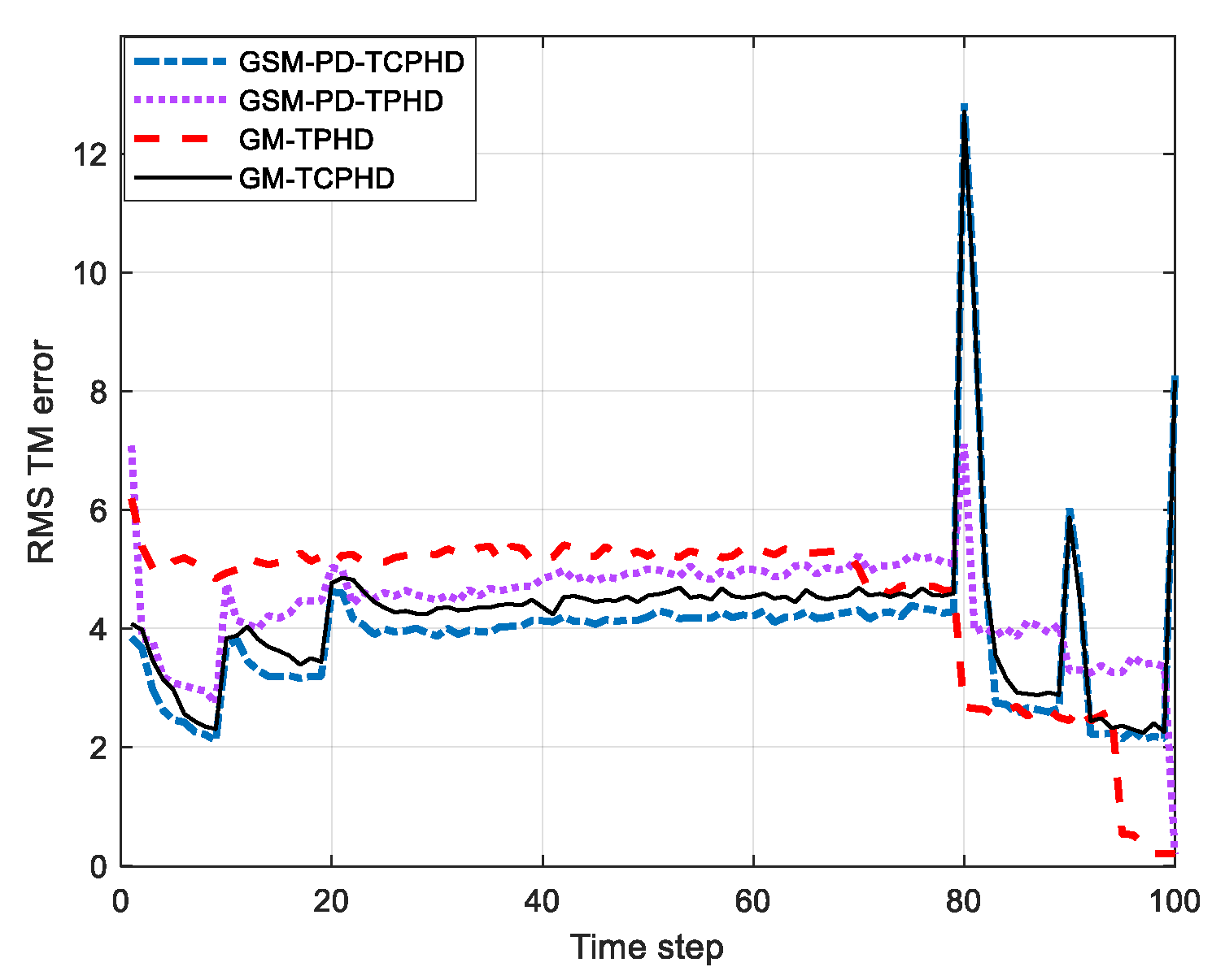
where ${\tilde{\mathbf{X}}}_{k,i}$ is the estimated trajectories in the $i$th Monte Carlo experiments at time $k$. The Gaussian sequential mixture implementation of PD-TPHD and PD-TCPHD filters are named GSM-PD-TPHD and GSM-PD-TCPHD for short. The Gaussian mixture implementations of the TPHD and TCPHD filters are named GM-TPHD and GM-TCPHD for short. The output of GSM-PD-TPHD, GSM-PD-TCPHD, and the true trajectories are presented in Figure 1, and the value of $L$ is set as 4, and the mean number of clutter measurements is $N_c=50$. The numbers of targets are labeled in black, and the arrows indicate the directions of the movement of targets. It can be observed that the two proposed filters both generate the estimated trajectories at different time steps. Since there are no track switches and few false and missed targets in Figure 1, the two filters exhibit excellent performance under the cluttered condition.

In the next simulation, we provide the RMSE metric of trajectories for GSM-PD-TPHD, GSM-PD-TCPHD, GM-TPHD, and GM-TCPHD filters in Figure 2. Figure 2 shows that PD-TPHD has a lower error than TPHD, and PD-TCPHD also has a lower error than TCPHD. The reason lies in the fact that PD-TPHD and PD-TCPHD contain augmented measurements, enhancing the precision of filtering.

In addition, the estimated cardinality for the two proposed filters is shown in Figure 3. As GSM-PD-TCPHD propagates the cardinality distribution in the recursive filtering, which matches the second moment, GSM-PD-TCPHD possesses a more accurate estimation of cardinality than GSM-PD-TPHD unless the number of targets decreases instantaneously. The phenomena can be illustrated by the filters’ need for response time to adapt to the changes in cardinality. In addition, due to lower variance in the estimation of cardinality, GSM-PD-TCPHD and GM-TCPHD filters exhibit a lagging response to cardinality changes on average. That is, they are not easily influenced by the changes, resulting in a higher penalization for errors in the estimated cardinality, as confirmed in Figure 3.

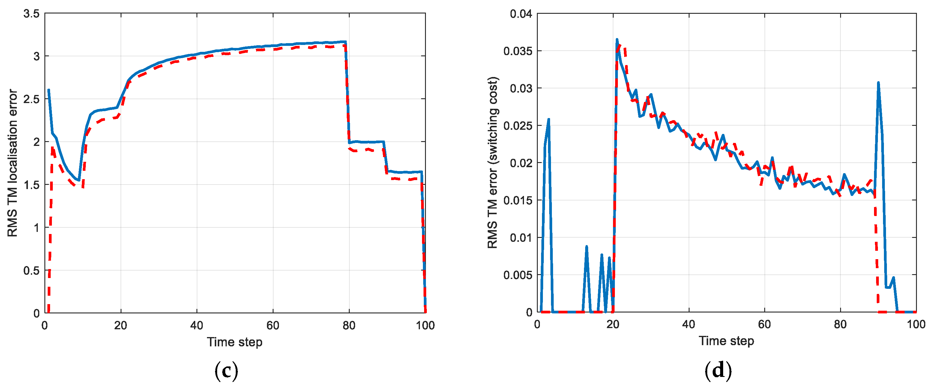
The RMSE metric of trajectories for two proposed filters is decomposed to analyze the performance of MTT in Figure 4. We observe that GSM-PD-TCPHD shows lower errors for missed targets than GSM-PD-TPHD. Regarding localization errors, false targets, and track switches, both filters exhibit similar accuracy, except when targets disappear at time steps 80 and 90.

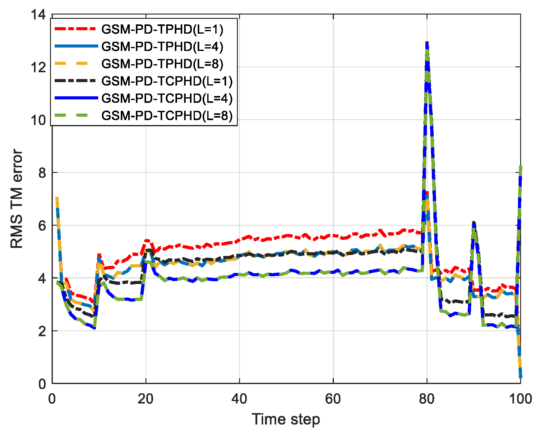
In order to evaluate the influence of $L$ on tracking performance, the RMSE of trajectories with different $L=\{\mathrm{1,4},8\}$ for two proposed filters is depicted in Figure 5. From Figure 5, we observe that the RMSE of trajectories decreases with $L$ increase. When $L$ reaches a certain value, the enhancement becomes less distinct. It should be noted that $L$ has no impact on the start and end times of the estimated trajectories.

Due to the increasing value of $L$, the computational burden should be considered. The running times of the filters with a 2.5 GHz Intel i5 laptop are displayed in

Table 2. The running time(s) of the filters.

$L$	1	2	4	8	15	30
PD-TPHD	1.85	1.93	2.09	2.52	3.66	8.05
PD-TCPHD	2.21	2.31	2.52	3.11	4.33	9.55
TPHD	1.47	1.53	1.68	1.81	2.51	5.26
TCPHD	1.78	1.83	1.97	2.26	2.83	5.56

.

From Table 2, the running times of the two proposed filters are all longer than those of the TPHD and TCPHD filters. The reason is that PD-TPHD and PD-TCPHD filters contain dimension expansion measurements, although the sequential process is utilized to deal with the measurements of location and Doppler separately, refraining from operating on the high-dimensional sets directly. When the value of $L$ is larger than 8, the running time increases sharply, while the enhancement of performance is not distinct from $L=4$. Hence, considering the balance between the performance of the algorithm and the computational burden, $L=4$ is a suitable choice for both filters in such a scenario, and the running times of the proposed filters are slightly longer than the other filters.

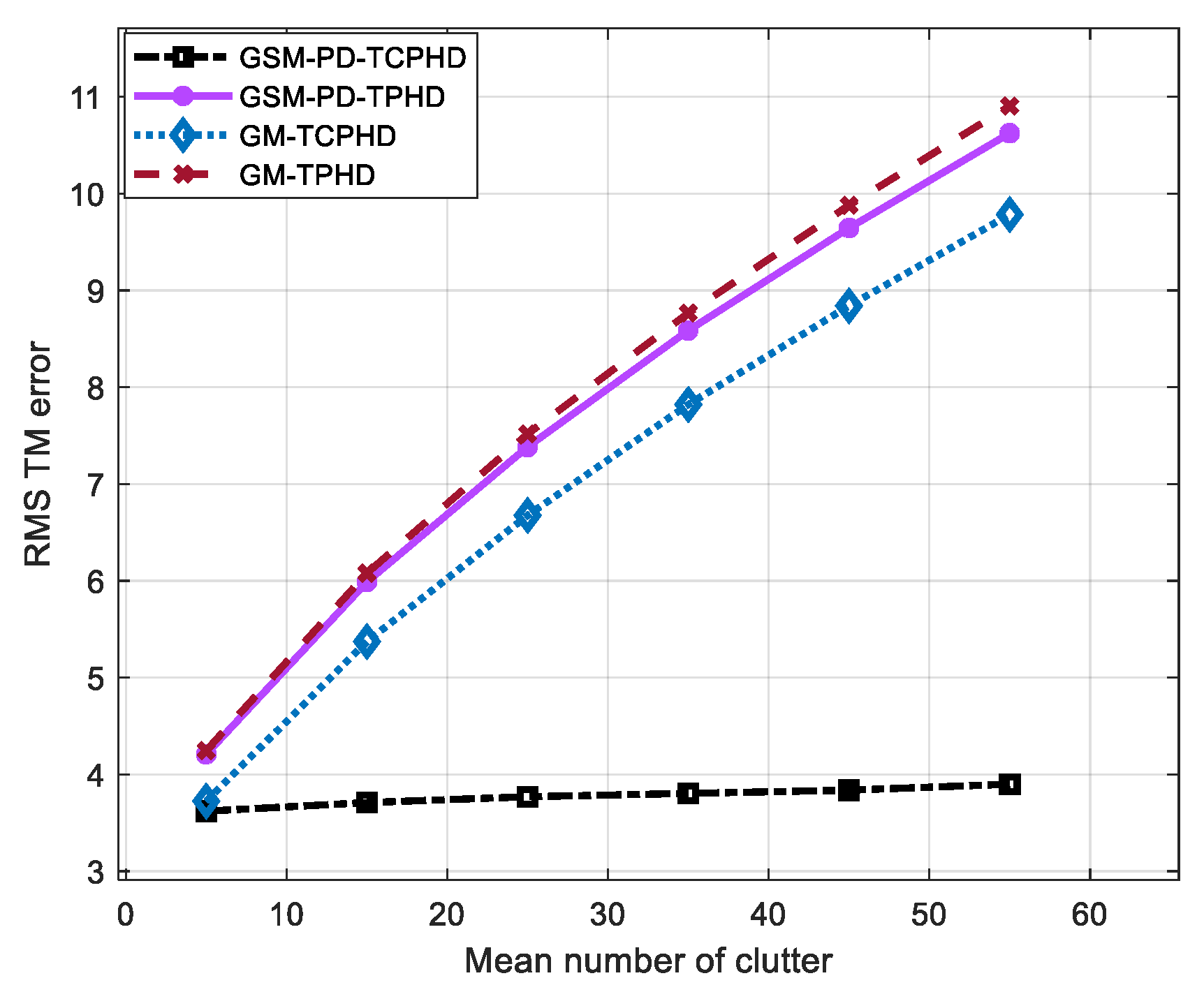
Additionally, we concentrate on assessing the effectiveness of incorporating Doppler information into GSM-TPHD and GSM-TCPHD for clutter suppression and performance improvement. The RMSE of trajectories under different clutter densities is presented in Figure 6. As shown in Figure 6, the augmentation of Doppler enhances the performance of two proposed filters notably. The improvement in MTT is more obvious with the increase in clutter density.

6. Conclusions

In this paper, the trajectory of PHD and CPHD filters for the pulse Doppler radar are developed. To address the multi-trajectory tracking in scenarios with clutter, we utilize the Doppler measurement model to reconstruct the measurement model and derive the updated steps of both filters. Furthermore, the Gaussian sequential mixture implementations of both filters are also derived, which guarantees the tracking performance at the cost of computational complexity. For the sake of reducing the computational burden, the $L$-scan approximations of both filters are provided. The value of $L$ has an impact on the estimation of target localization. Finally, simulation experiments prove that the proposed filters are superior to the TPHD and TCPHD filters in scenarios with clutter, which perform better estimates of trajectories.

References

1. Popp, R.L.; Kirubarajan, T.; Pattipati, K.R. Multitarget Multisensor Tracking: Applications and Advances III; Artech House: Norwood, MA, USA, 2000. [Google Scholar]
2. Ainsleigh, P.L.; Luginbuhl, T.E.; Willett, P.K. A sequential target existence statistic for joint probabilistic data association. IEEE Trans. Aerosp. Electron. Syst. 2021, 57, 371–381. [Google Scholar] [CrossRef]
3. Liang, S.; Zhu, Y.; Gong, M.G.; Yan, J.K. Cauchy-Schwarz divergence-based set joint probabilistic data association filter for tracking multiple objects in cluttered environment. IEEE Trans. Geosci. Remote Sens. 2023, 62, 5100915. [Google Scholar] [CrossRef]
4. Blackman, S.S. Multiple hypothesis tracking for multiple target tracking. IEEE Trans. Aerosp. Electron. Syst. 2004, 19, 5–18. [Google Scholar] [CrossRef]
5. Sheng, H.; Chen, J.H.; Zhang, Y.; Ke, W.; Xiong, Z.; Yu, J.Y. Iterative multiple hypothesis tracking with tracklet-level association. IEEE Trans. Circuits Syst. Video Technol. 2019, 29, 3660–3672. [Google Scholar] [CrossRef]
6. Du, R.Z.; Liu, L.; Bai, X.R.; Zhou, F. A new scatterer trajectory association method for ISAR image sequence utilizing multiple hypothesis tracking algorithm. IEEE Trans. Geosci. Remote Sens. 2021, 60, 5103213. [Google Scholar] [CrossRef]
7. Mahler, R. Statistical Multisource Multitarget Information Fusion; Artech House: Norwood, MA, USA, 2007. [Google Scholar]
8. Mahler, R. Multitarget Bayes filtering via first-order multitarget moments. IEEE Trans. Aerosp. Electron. Syst. 2003, 39, 1152–1178. [Google Scholar] [CrossRef]
9. Vo, B.-N.; Ma, W.-K. The Gaussian mixture probability hypothesis density filter. IEEE Trans. Signal Process. 2006, 54, 4091–4104. [Google Scholar] [CrossRef]
10. Vo, B.-N.; Singh, S.; Doucet, A. Sequential Monte Carlo methods for multi-target filtering with random finite sets. IEEE Trans. Aerosp. Electron. Syst. 2005, 41, 1224–1245. [Google Scholar] [CrossRef]
11. Mahler, R. PHD filters of higher order in target number. IEEE Trans. Aerosp. Electron. Syst. 2007, 43, 1523–1543. [Google Scholar] [CrossRef]
12. Vo, B.-N.; Cantoni, A. Analytic implementations of the cardinalized probability hypothesis density filter. IEEE Trans. Signal Process. 2007, 55, 3553–3567. [Google Scholar] [CrossRef]
13. Jones, B.-A. CPHD filter birth modeling using the probabilistic admissible region. IEEE Trans. Signal Process. 2018, 54, 1456–1469. [Google Scholar] [CrossRef]
14. Vo, B.-T.; Vo, B.-N.; Cantoni, A. The cardinality balanced multi-target multi-Bernoulli filter and its implementations. IEEE Trans. Signal Process. 2009, 57, 409–423. [Google Scholar] [CrossRef]
15. Williams, J.L. An efficient, variational approximation of the best fitting multi-Bernoulli filter. IEEE Trans. Signal Process. 2015, 63, 258–273. [Google Scholar] [CrossRef]
16. Vo, B.-T.; Vo, B.-N. Labeled random finite sets and multi-object conjugate priors. IEEE Trans. Signal Process. 2013, 61, 3460–3475. [Google Scholar] [CrossRef]
17. Vo, B.-N.; Vo, B.-T.; Phung, D. Labeled random finite sets and the Bayes multi-target tracking filter. IEEE Trans. Signal Process. 2014, 62, 6554–6567. [Google Scholar] [CrossRef]
18. Reuter, S.; Vo, B.-T.; Vo, B.-N.; Dietmayer, K. The labeled multi-Bernoulli filter. IEEE Trans. Signal Process 2014, 62, 3245–3260. [Google Scholar] [CrossRef]
19. Papi, F.; Vo, B.-N.; Vo, B.-T.; Fantacci, C.; Beard, M. Generalized labeled multi-Bernoulli approximation of multi-object densities. IEEE Trans. Signal Process. 2015, 63, 5487–5497. [Google Scholar] [CrossRef]
20. David, F.C. On implementing 2D rectangular assignment algorithms. IEEE Trans. Aerosp. Electron. Syst. 2016, 52, 1679–1696. [Google Scholar] [CrossRef]
21. Vo, B.-N.; Vo, B.-T.; Hung, G.H. An efficient implementation of the generalized labeled multi-Bernoulli filter. IEEE Trans. Signal Process. 2017, 65, 1975–1987. [Google Scholar] [CrossRef]
22. Vo, B.-N.; Vo, B.-T. A multi-scan labeled random finite set model for multi-object state estimation. IEEE Trans. Signal Process. 2019, 67, 4948–4963. [Google Scholar] [CrossRef]
23. Petetin, Y.; Desbouvries, F. Bayesian multi-object filtering for pairwise Markov chains. IEEE Trans. Signal Process. 2013, 61, 4481–4490. [Google Scholar] [CrossRef]
24. Pieczynski, W.; Desbouvries, F. Kalman Filtering using Pairwise Gaussian Models. In Proceedings of the 2003 IEEE International Conference on Acoustics, Speech and Signal Processing, Hong Kong, China, 6 April 2003. [Google Scholar]
25. Liu, J.; Wang, C. Cardinalized probability hypothesis density filter based on pairwise Markov chains. J. Electron. Inf. Technol. 2019, 41, 492–497. [Google Scholar] [CrossRef]
26. Zhang, G.-H.; Han, C.-Z.; Lian, F.; Zeng, L.-H. Cardinality balanced multi-target multi-Bernoulli filter for pairwise Markov model. Acta Autom. Sin. 2017, 43, 2100–2108. [Google Scholar] [CrossRef]
27. Mahler, R. The pairwise-Markov Bernoulli filter. IEEE Access 2020, 8, 168229–168245. [Google Scholar] [CrossRef]
28. Mahler, R. Bernoulli filters for multiple correlated sensors. IEEE Access 2021, 9, 2310–2316. [Google Scholar] [CrossRef]
29. Zhou, Y.; Yan, L.; Li, H.; Xia, Y. The multiple pairwise Markov chain model-based labeled multi-Bernoulli filter. J. Franklin Inst 2024, 361, 106939. [Google Scholar] [CrossRef]
30. Kim, H.; Granstrom, K.; Gao, L.; Battistelli, G.; Kim, S.; Wymeersch, H. 5G mmWave cooperative positioning and mapping using multi-model PHD filter and map fusion. IEEE Trans. Wirel. Commun. 2020, 19, 3782–3795. [Google Scholar] [CrossRef]
31. Ramachandran, R.K.; Fronda, N.; Sukhatme, G.S. Resilience in multirobot multitarget tracking with unknown number of targets through reconfiguration. IEEE Trans. Control Netw. Syst. 2021, 8, 609–620. [Google Scholar] [CrossRef]
32. Gao, L.; Battistelli, G.; LChisci, L. Random-finite-set-based distributed multirobot SLAM. IEEE Trans. Robot. 2020, 36, 1758–1777. [Google Scholar] [CrossRef]
33. Li, G.C.; Li, G.; He, Y. Distributed GGIW-CPHD-based extended target tracking over a sensor network. IEEE Signal Process. Lett. 2022, 29, 842–846. [Google Scholar] [CrossRef]
34. Gao, L.; Battistelli, G.; Chisci, L. Multiobject fusion with minimum information loss. IEEE Signal Process. Lett. 2020, 27, 201–205. [Google Scholar] [CrossRef]
35. Gao, L.; Battistelli, G.; Chisci, L.; Wei, P. Distributed joint sensor registration and multitarget tracking via sensor network. IEEE Trans. Aerosp. Electron. Syst. 2019, 56, 1301–1317. [Google Scholar] [CrossRef]
36. Yu, B.R.; Li, T.C.; Ge, S.J.; Gu, H. Robust CPHD fusion for distributed multitarget tracking using asynchronous sensors. IEEE Sens. J. 2021, 22, 1030–1040. [Google Scholar] [CrossRef]
37. García-Fernández, Á.F.; Svensson, L. Trajectory PHD and CPHD filters. IEEE Trans. Signal Process. 2019, 67, 5702–5714. [Google Scholar] [CrossRef]
38. García-Fernández, Á.F. Derivation of the PHD and CPHD filters based on direct Kullback-Leibler divergence minimization. IEEE Trans. Signal Process. 2015, 63, 5812–5820. [Google Scholar] [CrossRef]
39. García-Fernández, Á.F.; Svensson, L. Trajectory probability hypothesis density filter. In Proceedings of the 21st International Conference on Information Fusion, Cambridge, UK, 10–13 July 2018. [Google Scholar]
40. García-Fernández, Á.F.; Svensson, L.; Williams, J.L.; Xia, Y.; Granström, K. Trajectory Poisson Multi-Bernoulli Filters. IEEE Trans. Signal Process. 2020, 68, 4933–4945. [Google Scholar] [CrossRef]
41. García-Fernández, Á.F.; Svensson, L. Tracking Multiple Spawning Targets Using Poisson Multi-Bernoulli Mixtures on Sets of Tree Trajectories. IEEE Trans. Signal Process. 2022, 70, 1987–1999. [Google Scholar] [CrossRef]
42. García-Fernández, Á.F.; Ralph, J.; Horridge, P.; Maskell, S. Gaussian trajectory PMBM filter with nonlinear measurements based on posterior linearization. In Proceedings of the 25th International Conference on Information Fusion, Linköping, Sweden, 4 July 2022. [Google Scholar]
43. Wang, X.; Musicki, D.; Ellem, R. Efficient and enhanced multi-target tracking with Doppler measurements. IEEE Trans. Aerosp. Electron. Syst. 2009, 45, 1400–1417. [Google Scholar] [CrossRef]
44. Zhang, S.; Bar-Shalom, Y. Track segment association for GMTI tracks of evasive move-stop-move maneuvering targets. IEEE Trans. Aerosp. Electron. Syst. 2011, 47, 1899–1914. [Google Scholar] [CrossRef]
45. Georgescu, R.; Willett, P. Predetection fusion with Doppler measurements and amplitude information. IEEE J. Ocean. Eng. 2012, 37, 56–65. [Google Scholar] [CrossRef]
46. Wu, W.H.; Jiang, J.; Liu, W.J.; Qin, X.; Zhang, W. A sequential converted measurement Kalman filter in the ECEF coordinate system for airborne Doppler radar. Aerosp. Sci. Technol. 2016, 51, 11–17. [Google Scholar] [CrossRef]
47. Ouellette, J.D.; Bounds, W.T.; Dowgiallo, D.J.; Toporkov, J.V.; Hwang, P.A. On the sensitivity of passive multistatic radar amplitude and Doppler measurements to significant wave height. IEEE Geosci. Remote Sens. 2021, 19, 3503105. [Google Scholar] [CrossRef]
48. McLinden, M.L.W.; Loftus, A.M.; Li, L.; Heymsfield, G.M. Application of nonuniform beam filling Doppler velocity error correction on airborne radar measurements. IEEE Geosci. Remote Sens. 2021, 19, 3509905. [Google Scholar] [CrossRef]
49. Yoon, J.H.; Kim, D.Y.; Bae, S.H.; Shin, V. Joint initialization and tracking of multiple moving objects using doppler information. IEEE Trans. Signal Process. 2011, 59, 3447–3452. [Google Scholar] [CrossRef]
50. Saurav, S.; Yimin, D.Z.; Moeness, G.A.; Braham, H. Group sparsity based multi-target tracking in passive multi-static radar systems using doppler-only measurements. IEEE Trans. Signal Process. 2016, 64, 3619–3634. [Google Scholar] [CrossRef]
51. Francesco, P. Multi-sensor δ—GLMB filter for multi-target tracking using Doppler only measurements. In Proceedings of the European Intelligence and Security informatics Conference, Manchester, UK, 7–9 September 2015. [Google Scholar]
52. Wu, W.H.; Jiang, J.; Liu, W.J.; Feng, X.; Gao, L.; Qin, X. Augmented state GM-PHD filter with registration errors for multi-target tracking by Doppler radars. Signal Process. 2016, 120, 117–128. [Google Scholar] [CrossRef]
53. Zheng, S.Y.; Jiang, L.B.; Yang, Q.W.; Zhao, Y.J.; Wang, Z. Adaptive PHD filter with RCS and Doppler feature for space targets tracking via space-based radar. IEEE Trans. Aerosp. Electron. Syst. 2024, 60, 3750–3765. [Google Scholar] [CrossRef]
54. Wang, H.B.; Zhao, T.Z.; Wu, W.H.; Lu, M.L.; Xiong, L. The multi-target tracking algorithm based on the MM-GLMB filter with Doppler information. In Proceedings of the 4th International Conference on Robotics, Control and Automation Engineering, Wuhan, China, 4–6 November 2021. [Google Scholar]
55. García-Fernández, Á.F.; Rahmathullah, A.S.; Svensson, L. A metric on the space of finite sets of trajectories for evaluation of multi-target tracking algorithms. IEEE Trans. Signal Process. 2020, 68, 3917–3928. [Google Scholar] [CrossRef]
Figure 1. The trajectory of filters at time steps 43 and 75. (a) The trajectory of PD-TPHD at time step 43. (b) The trajectory of PD-TPHD at time step 75. (c) The trajectory of PD-TCPHD at time step 43. (d) The trajectory of PD-TCPHD at time step 75.
Remotesensing 16 04671 g001
Figure 2. The RMSE of trajectories for GSM-PD-TPHD, GSM-PD-TCPHD, GM-TPHD, and GM-TCPHD filters.
Remotesensing 16 04671 g002
Figure 3. The estimated cardinality of GSM-PD-TPHD and GSM-PD-TCPHD filters.
Remotesensing 16 04671 g003
Figure 4. The RMSE of the filters. (a) The RMSE for missed targets. (b) The RMSE for false targets. (c) The RMSE for localization. (d) The RMSE for track switches.
Remotesensing 16 04671 g004aRemotesensing 16 04671 g004b
Figure 5. The RMSE of trajectories with different L for GSM-PD-TPHD and GSM-PD-TCPHD filters.
Remotesensing 16 04671 g005
Figure 6. The RMSE of trajectories with different clutter densities.
Remotesensing 16 04671 g006