Abstract
Land surface temperature (LST) plays a pivotal role in many environmental sectors. Unfortunately, thermal bands produced by instruments that are onboard satellites have limited spatial resolutions; this seriously impairs their potential usefulness. In this study, we propose an automatic procedure for the spatial downscaling of the two 100 m thermal infrared (TIR) bands of LandSat 8/9, captured by the TIR spectrometer (TIRS), by exploiting the bands of the optical instrument. The problem of fusion of heterogeneous data is approached as hypersharpening: each of the two sharpening images is synthesized following data assimilation concepts, with the linear combination of 30 m optical bands and the 15 m panchromatic (Pan) image that maximizes the correlation with each thermal channel at its native 100 m scale. The TIR bands resampled at 15 m are sharpened, each by its own synthetic Pan. On two different scenes of an OLI-TIRS image, the proposed approach is compared with 100 m to 15 m pansharpening, carried out uniquely by means of the Pan image of OLI and with the two high-resolution assimilated thermal images that are used for hypersharpening the two TIRS bands. Besides visual evaluations of the temperature maps, statistical indexes measuring radiometric and spatial consistencies are provided and discussed. The superiority of the proposed approach is highlighted: the classical pansharpening approach is radiometrically accurate but weak in the consistency of spatial enhancement. Conversely, the assimilated TIR bands, though adequately sharp, lose more than 20% of radiometric consistency. Our proposal trades off the benefits of its counterparts in a unique method.
1. Introduction
Land surface temperature (LST) is an important parameter that modulates surface energy fluxes. Its relevance for environmental remote sensing has been widely recognized [1]. Typical applications of LST concern soil moisture estimation [2], forest fire detection [3], surface urban heat island monitoring [4], studies of hydrological processes [5], and climate studies [6]. Before the advent of satellites, it was extremely difficult to obtain LST in extended areas. Even today, it is difficult, and often impossible, to acquire satellite LST with high spatial resolution while maintaining a radiometric quality suitable for most applications. The temporal resolution, crucial for early detection of forest fires [3], is always accompanied by a reduced spatial resolution due to the height of the geosynchronous platform. This low spatial resolution results in a thermal mixture in which pixel sizes are larger than elements with homogeneous thermal properties. Thus, LST downscaling becomes a key topic in environmental remote sensing. Whenever the enhancement in spatial resolution is achieved by means of one or more observations of the same scene capable of resolving finer details, the downscaling is approached as a problem of multi-sensor image fusion. In fact, the fusion of images captured by heterogeneous sensors, a.k.a., multimodal fusion, is widespread in the field of medical imaging [7]. Multimodal fusion has two distinct strands in the field of remote sensing: fusion of data taken by optical and active microwave sensors and fusion of optical and thermal scanner data, as in the present study.
Thermal sensors capture the electromagnetic radiation emitted by the Earth’s surface depending on its temperature, following Planck’s law and emissivity coefficient. Since the radiant exitance of the Earth at environmental temperature is low and thermal detectors are considerably noisy due to large fluctuations of the dark current, the spatial resolution of thermal infrared (TIR) images is unavoidably scarce for the collection of a sufficient number of incoming photons. The easiest way to improve the signal-to-noise ratio (SNR) consists of increasing the elementary area of integration of the detector, thus reducing its spatial resolution capability. Hence, the usefulness of increasing the spatial resolution of TIR acquisitions is evident.
The enhancement in spatial resolution for TIR imagery is not trivial. In fact, the TIR spectral channels do not overlap with those of other bands with higher spatial resolution that could be exploited for spatial sharpening [8]. Spectral overlap would entail some cross-correlation between sharpened (master) and sharpening (slave) images, as happens for multispectral (MS) pansharpening, and cross-correlation is the prerequisite for fusion. In principle, there is no evidence that TIR and visible and near infrared (VNIR) spectral radiances are cross-correlated, with the former being emitted and the latter reflected by Earth’s surface illuminated by sunlight. The imaging mechanism occurs in disjoint spectral intervals: the wavelengths of TIR are at least 10 times larger than those of VNIR.
To overcome the lack of spectral overlap, several scientists have addressed the problem of spatial resolution enhancement of TIR images by exploiting physical relationships between the TIR bands and other bands featuring a higher spatial detail. A notable example is the relationship observed between vegetation and temperature. A viable strategy is to calculate the normalized differential vegetation index (NDVI) as a downscaling factor to infer TIR images at higher spatial resolutions [9]. NDVI is calculated from the red and NIR bands that are usually available with a spatial resolution better than TIR [10]. This idea was developed by Kustas et al. [11], improved by Agam et al. [12], and revisited by Jeganathan [13] and Chen et al. [14]. In detailed urban environments, the coupling of the NDVI with the surface albedo has also been proposed [15].
Later [16], the problem of resolution enhancement of TIR images was formulated in terms of disaggregation of remote-sensing LST (DLST). Two subtopics, thermal sharpening (TSP) [17] and temperature unmixing (TUM) [18], were identified as a dual pair of DLST. TSP refers to any kind of procedure by which TIR images are spatially enhanced for the purpose of interpretation using spatially distributed auxiliary data that are statistically correlated with LST on the basis of pixel, block, or region [19]. Instead, TUM indicates the procedures by which the temperatures of the elementary components within a pixel are decomposed on the basis of temporal, spatial, spectral, or angular observations [16]. This approach has recently been used in a spatio-temporal context to monitor temperature in urban areas [20].
Several fundamental assumptions are usually adopted in DLST:
- 1.
- Pixels are larger than image objects and thus the surface should not be thermally homogeneous at the pixel scale (heterogeneity);
- 2.
- At the object scale, the surface is assumed isothermal (separability) [19];
- 3.
- Auxiliary data relating to the physical properties of subpixel elements are available (connectivity);
- 4.
- Aggregation occurring among objects is additive (additivity) [19].
The first assumption implies that a pixel consists of an array of components that characterize the mixture among multiple elements. The second is unrealistic but is assumed to be true in most previous studies. The third assumption is necessary to keep the number of unknowns as small as possible because such auxiliary data can be used to determine the fractions of elements or to estimate the physical properties of elements. The last assumption is mostly reasonable when there is no energy interaction among components, but the aggregation is generally nonlinear when heterogeneous surfaces have a significant three-dimensional structure, much larger than the measuring wavelength, which may cause some intershadows and thus create nonlinear interactions between subfacets [21]. An in-depth insight on DLST methods and a thorough collection of references can be found in the seminal paper by Zhan et al. [16] and in the up-to-date comprehensive review by Firozjaei et al. [22].
Upon these premises, our study introduces an original approach that can be adopted for sharpening TIR data and hence for the downscaling of LST maps. The method belongs to the TSP family and exploits the presence of a statistical similarity between TIR and some of the other higher-resolution bands, as originally proposed by Aiazzi et al. [8]. Due to the interesting spectral characteristics of a recent instrument, including the presence of multiple TIR bands, a specific case study concerning LandSat 8/9 data will be presented and discussed. The main novelty consists of the use of the hypersharpening paradigm [23]. Regardless of the existence and uniqueness of a sharpening image, as for pansharpening, hypersharpening deals with the synthesis of an ideal sharpening image tailored to specific characteristics of each of the bands that shall be sharpened. In substance, hypersharpening can be regarded within the context of data assimilation theory, which has been used for thermal sharpening [24,25]. Extensions to different multi-platform instruments have recently been proposed within the context of a unimodal fusion, thermal–thermal [26] or optical–optical [27], between homogeneous datasets. This approach is an alternative to much more complicated, yet valuable, learning-based approaches that are useful for spatio-temporal fusion [28]. The versatility of generative adversarial networks (GANs) [29] has recently been recognized for the synthesis of remote sensing images [30].
The remainder of this article is organized as follows. Section 2 illustrates the thermal and optical data and analyzes their inter-channel correlation; then, hypersharpening is introduced and the assimilation procedure of the sharpening bands is described, together with the sharpening rule, and statistical indexes of thermal and spatial consistency are reviewed. Section 3 presents the results of two scenes of a large OLI-TIRS image collected from LandSat 9. Section 4 discusses the results and draws guidelines for the interpretation of results from a disaggregation perspective. Eventually, the concluding remarks and possible future developments are outlined in Section 5.
2. Materials and Methods
2.1. LandSat 8/9 OLI and TIRS
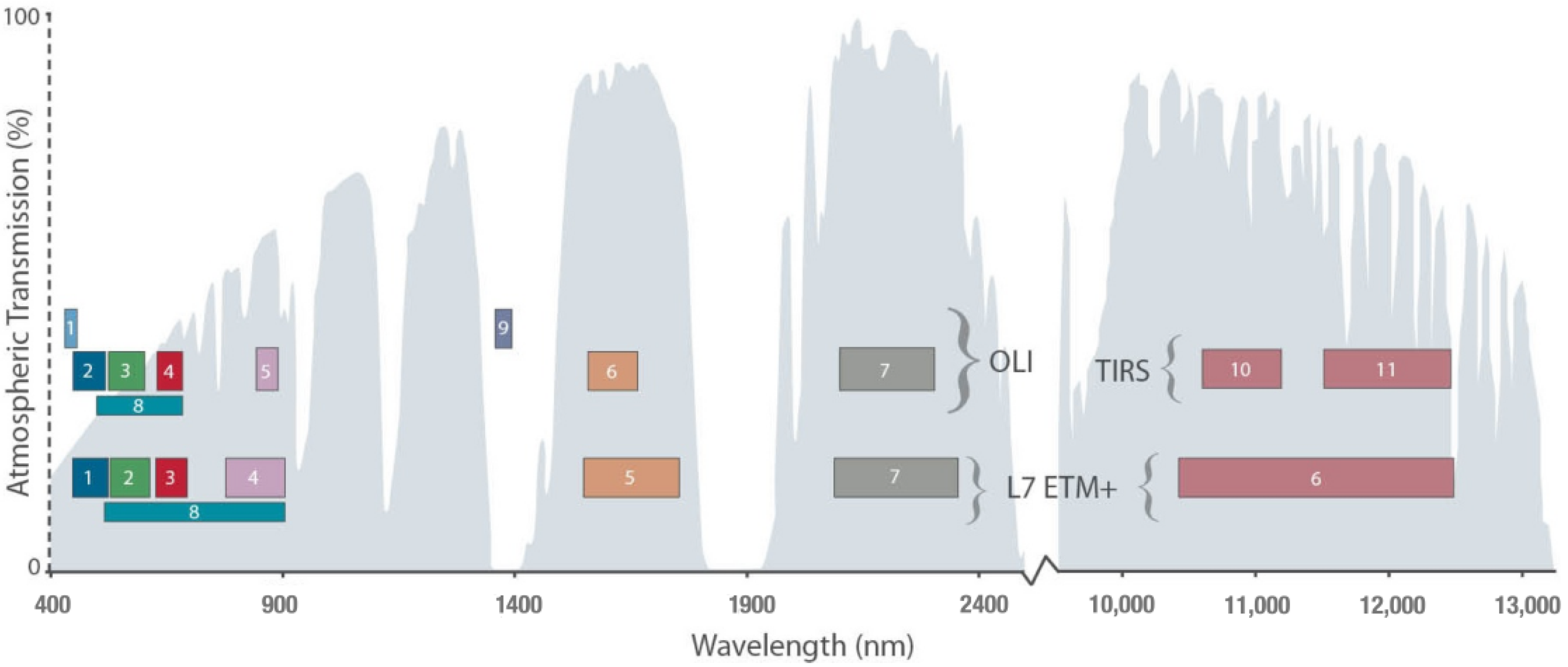
The operational land imager OLI, onboard NASA/USGS LandSat 8 and LandSat 9, provides high-resolution images of our planet in eleven different bands of the electromagnetic spectrum, ranging from visible to thermal radiation, the latter thanks to the TIR spectrometer (TIRS). The resolution, or more precisely the spatial sampling interval (SSI), of image products ranges between 15 and 100 m. OLI/TIRS data are used to create detailed maps of surface temperature, emissivity, spectral reflectance, and elevation. Analogous to LandSat “enhanced thematic mapper plus” (ETM+), OLI features a panchromatic (Pan) channel, whose spectral coverage has been specifically devised to expedite the sharpening of the thermal bands, with two instead of one. Figure 1 presents a synoptic comparison of the two instruments: in addition to the narrow-band Pan of OLI, differences are the coastal and cirrus bands, suitable for atmosphere studies, and the split of the unique thermal band of ETM+ to allow for thermal diversity. The bands of OLI, including TIRS, are described in Table 1. There are three groups of bands in three different spectral ranges, VNIR, short wave infrared (SWIR), and TIR, with different spatial resolutions.

Figure 1.
Comparison of spectral bands of OLI/TIRS onboard LandSat 8/9 and ETM+ onboard LandSat 7, with atmospheric transmission window superimposed (available online: https://landsat.gsfc.nasa.gov/satellites/landsat-8/ (accessed on 19 October 2024)).

Table 1.
Characteristics of the eleven spectral bands of OLI and TIRS instruments onboard LandSat 8/9.
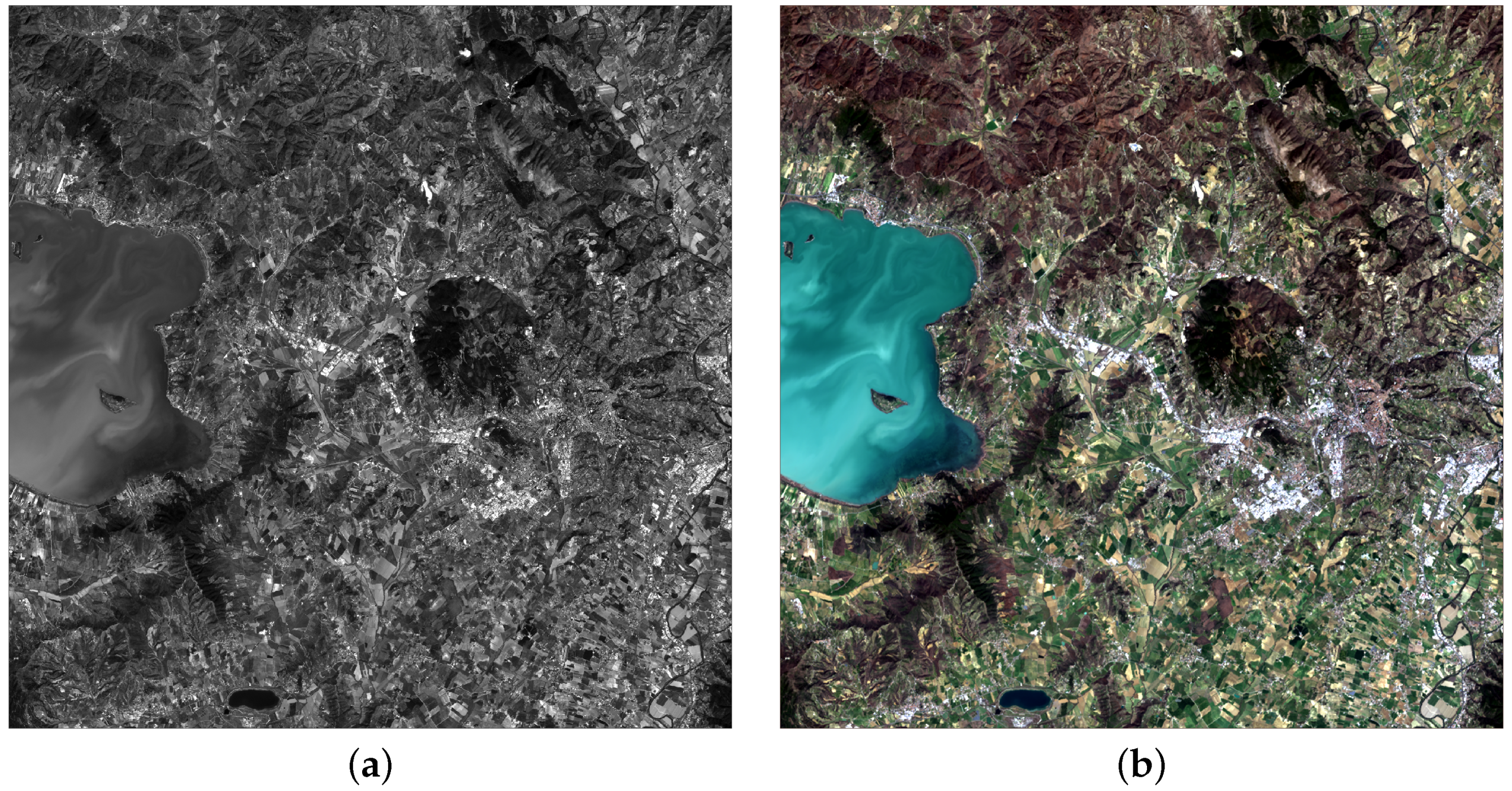
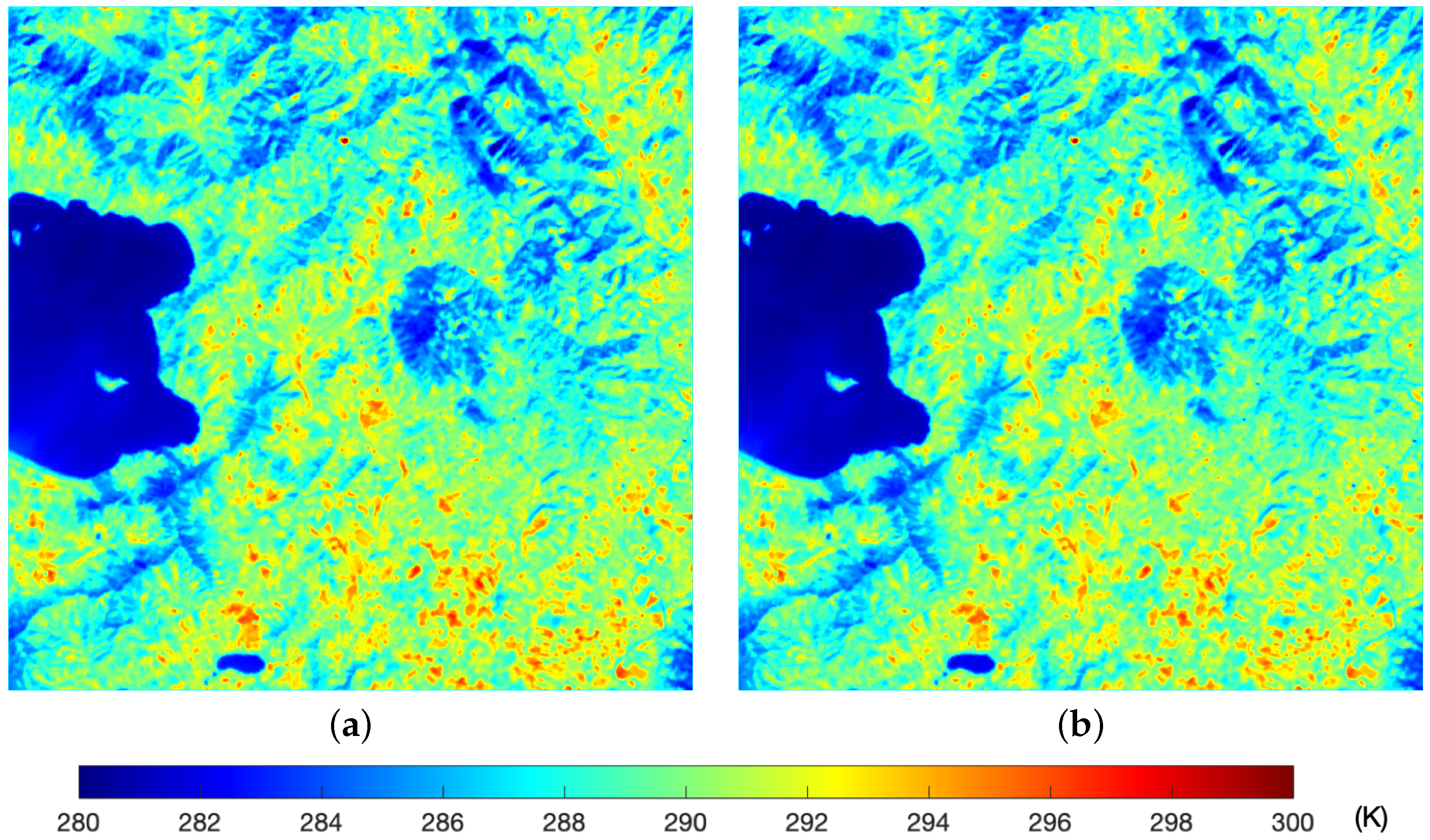
A LandSat 9 scene was acquired near Perugia, in Central Italy, on 22 March 2022. The geographical position of the test image is shown in Figure 2. Figure 3 displays the whole scene: 15 m Pan (B8) and true color composition of B4, B3, and B2, interpolated at 15 m. In addition to the lake, the scene includes a built-up area and a surrounding vegetated region. As it appears, the optical acquisition is perfectly cloud-free. Figure 4 shows the two thermal bands, B10 and B11, displayed as absolute temperature maps with the associated color palette. The TIRS data are delivered and displayed in LST format, with measure unit K. For calculating correlations with the optical bands, and for subsequent fusion, they have been converted to surface spectral radiance units [W m−2sr−1μ−1] by using the file metadata to apply Planck’s law. The conversions of surface radiance to LST and of LST back to radiance would assume an average emissivity coefficient of the land surface equal to 0.97 (see https://earthexplorer.usgs.gov, (accessed on 19 October 2024)). This explains the singular effect that two adjacent TIR bands measure slightly different LSTs: the conversion coefficients to and from LST assume a constant emissivity equal to 0.97, which is an approximation of its unknown true value.
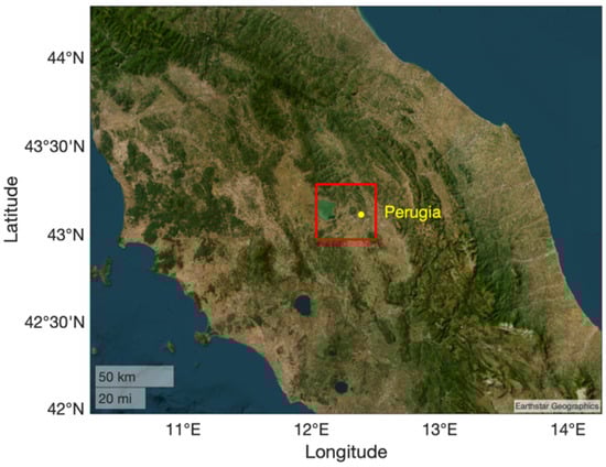
Figure 2.
Geographic map of Central Italy: the 30 km × 30 km test area is highlighted.

Figure 3.
The 30 km × 30 km LandSat 9 OLI acquisition: (a) Pan image (B8); (b) 15 m interpolated true color (B4-B3-B2).
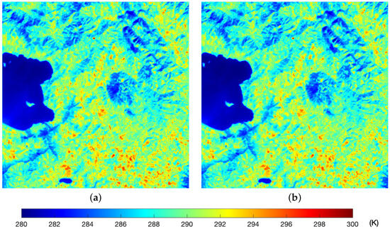
Figure 4.
The 30 km × 30 km original thermal bands at 100 m resolution: (a) B10; (b) B11.
The statistical similarity of the images to be merged is crucial for the quality of the fusion. Table 2 details the correlation matrix of the test image, calculated between the original TIR bands (B10 and B11), VNIR bands (B1, B2, B3, B4 and B5), SWIR bands (B6 and B7), panchromatic band (B8), and narrow cirrus band (B9), suitable for detecting ice crystals in atmosphere. The Pan band has been previously degraded at 30 m and 100 m resolutions retaining the original 15 m scale, i.e., pixel size, the former for calculating correlations with the other VNIR bands and the latter for correlations involving the two TIR bands. All 30 m optical bands have been resampled at 15 m scale and degraded at 100 m resolution. The correlation between two bands is trivially measured at the same spatial scale but also at the lower resolution, i.e., that of the less resolved band. Therefore, the band with greater spatial resolution must be spatially degraded by means of proper low-pass filters. As it appears, the optical bands are somewhat correlated, one with another, with the exception of the NIR band, which contains the radiation reflected by vegetation. The interpretation is made difficult by the presence of water pixels in the scene, whose response in the NIR and SWIR wavelengths is close to zero. This fact artificially increases the correlations of B5, B6, B7, and B9 towards TIR (B10 and B11) and decreases those of the visible bands, including B8 (Pan).
Table 2.
Correlation coefficients (CC) between LandSat 9 bands for the test image. The values above the main diagonal are computed for the entire scene, whereas the values below the diagonal are restricted to non-water pixels.
Given the relatively high correlation values of some bands, the strategy that appears to be a viable alternative to plain pansharpening would be using the 30 m VNIR/SWIR bands and the 15 m Pan (B8) for the synthesis of two sharpening bands, each tailored to the thermal features of a 100 m TIR band. In fact, if the correlation between the sharpening and the sharpened band is sufficiently high, the results of thermal fusion at 15 m are expected to be likely. This can be achieved by resorting to concepts of data assimilation to generate the synthetic bands and to the hypersharpening paradigm, which foresees as many sharpening images as there are bands that shall be sharpened.
2.2. Hypersharpening of TIRS Data
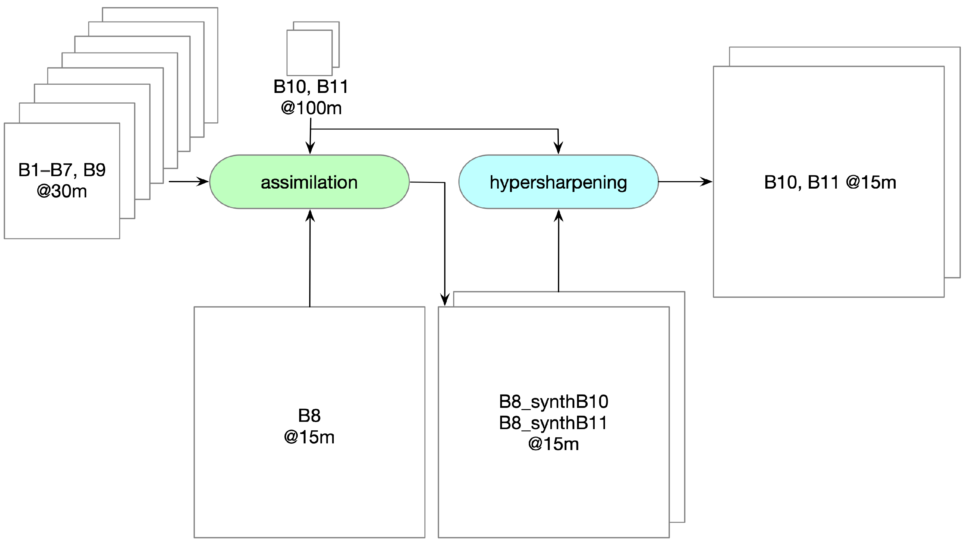
While pansharpening increases the geometric resolution of a multiband image by means of a Pan observation of the same scene with greater resolution, whenever the higher-resolution image is not unique, hypersharpening concerns the synthesis of a unique image from which the spatial details shall be extracted in order to optimize the products of fusion [23]. This synthetic Pan is generally different for each band that is enhanced. The idea is similar to predict the sharpening image through a hard or soft combination of a series of bands at higher resolution [31]. The combination can be driven by data assimilation concepts [25]. The wide choice of optical bands of OLI, including 15 m Pan, and the characteristics of the correlation matrix in Table 2 suggest exploiting the pixel-by-pixel combination of the optical bands according to the least squares (LS) coefficients of a multivariate regression of the optical bands towards each of the TIRS bands. Figure 5 outlines the flow diagram of the OLI/TIRS sharpening procedure: the synthetic high-resolution sharpening bands of each of the two TIRS bands are assimilated from the optical bands; the two synthetic Pans at 15 m are used for the hypersharpening of the TIR bands. Although the Pan image (B8) is unique, there are two different sharpening images, one for B10, one for B11.

Figure 5.
Flowchart ofthe proposed OLI + TIRS sharpening: hypersharpening provides the spatial enhancement of TIRS bands from 100 m to 15 m by injecting the high-pass spatial frequency components extracted from different synthetic sharpening images generated through assimilation of the optical bands, including the original 15 m Pan, to each of the thermal bands. The two assimilated bands at 15 m are also available as sharpened TIR bands.
Let denote the more spatially resolved bands, e.g., the eight 30 m VNIR bands of OLI and the 15 m Pan image, the former resampled at the scale of the latter (15 m) for homogeneity of notation. Let also indicate the bands having lower resolution, the TIRS bands, both at 100 m spatial resolution, and R the ratio of spatial scales of and (, , and , for OLI/TIRS). The sharpening band , of the ith band with lower resolution, , is synthesized as follows.
First, the bands are low-pass filtered with a frequency cutoff equal to , to yield the bands spatially degraded to the resolution of the bands that are being enhanced. The fractional scale ratio can be easily tackled by resorting to the generalized Laplacian pyramid [32], widely used for pansharpening [33]. Then, the relationships between the lower-resolution bands interpolated by R, , and are modeled as a multivariate linear regression:
in which is the space-varying residue. The set of optimal constant weights, , is calculated as the least squares (LS) solution of Equation (1). The spectral coefficients, , are used to synthesize the set of sharpening bands, :
The block labeled “assimilation” in the flowchart of Figure 5 performs the operations described in Equations (1) and (2).
Finally, the hypersharpened bands, , at a resolution of 15 m, can be computed by means of a projection-based fusion algorithm [34] between and :
in which and denote covariance and variance of random variables, is low-pass-filtered with 15/100 spatial frequency cutoff, or, equivalently,
Different models of detail injection, a contrast-based model [10] or a genetic model [35], can be adopted. The projection-based injection gain, defined as the ratio of covariance of source–destination to variance of source, measured at the spatial scale of the fusion product, 15 m, but at the resolution of the destination prior to fusion, that is, 100 m, can be calculated on a local sliding window in a space-varying fashion [36], instead of being global over the whole scene. The projection coefficient balances the injection of spatial details to the extent of correlation between the source of spatial details and the destination of such details. Note that Equation (3) denotes conventional pansharpening if is replaced with the original 15 m OLI Pan, , (B8) and with its low-pass version, .
Very and extremely high-resolution MS scanners, e.g., WorldView-3, in which four instruments with three different resolutions are present [37], may exhibit residual shifts due to uncorrected parallax views. In the case of LandSat 8/9, the negligible residual spatial shifts between the datasets allow for the use of fusion methods based on separable [38] or non-separable [39] multiresolution analysis of the sharpening image. Such methods are also recommended for merging data coming from different platforms [40,41].
The coefficient of determination (CD) of multivariate regression in Equation (1) measures the success of matching between each of the lower-resolution bands and the sharpening image synthesized from the higher-resolution VNIR/SWIR/Pan bands [42]. Note that the use of a multivariate regression to synthesize the sharpening band makes the method independent of the data format [43]. However, while the math derivation of the sharpening bands does not depend on the physical format of the data, e.g., top-of-atmosphere (TOA) spectral radiance or surface reflectance, provided that a linear affine relationship (straight line with slope and intercept) can be stated between the variables that appear in either the regression and in the fusion rule [43], the multiplicative injection gain derived from the radiative transfer model would assume that all band data are in a surface reflectance or a surface spectral radiance format without offset/intercept between variables due to atmospheric scattering effects. The surface reflectance is a level-two (L2) product and is usually distributed for global-coverage optical systems, such as OLI and Sentinel-2. The surface spectral radiance can be derived from the surface temperature format of TIRS data through the available metadata.
2.3. Assessment of Fusion Products
The empirical quality criteria of fusion products [44], used in the past also for thermal data [8], have been progressively abandoned in favor of consistency criteria embodied by several statistical indexes [45,46]. When fusion of heterogeneous data is concerned, consistency is suitable for quality evaluation. To provide a better view of the problem, we split the consistency property into two terms, which are given here with reference to the OLI-TIRS fusion problem:
- -
- Thermal consistency: the fused TIRS image, once spatially degraded at the original scale, should be as close as possible to the original TIRS image, i.e., the source of the thermal information;
- -
- Spatial consistency: the fused TIRS bands should be capable of synthesizing back the sharpening image.
Thermal and spatial consistencies are separately evaluated by the following metrics.
2.3.1. Normalized Root Mean Square Error (NRMSE)
The first index, named spectral consistency index for multiband images and radiometric consistency index for a unique band, will be referred to as the thermal consistency index. It is measured at the original resolution of TIRS but possibly at the scale of fusion products, i.e., at 100 m or at 15 m. All data, fused and reference, should be absolute temperatures expressed in K. The assimilated and fused TIRS bands are generated as surface spectral radiance and must be previously converted to surface temperature using the file metadata to invert Plank’s law. The consistency reference is the original 100 m TIRS, possibly interpolated at 15 m. The index, which measures a distortion, that is, a loss of consistency, is defined as the normalized root mean squared error (NRMSE), possibly expressed in percentage, between the TIRS band fused at 15 m spatially degraded to 100 m and the original 100 m TIRS band:
in which indicates the mean of the (interpolated) thermal band, , denotes the Frobenius norm, and the fused TIRS band after low-pass filtering. NRMSE is a distortion index; hence, its ideal value is zero. The index defined by Equation (5) should be as close to zero as possible to indicate that fusion does not change the original information [23], which is thermal in the present case. Instead of percentage NRMSE, the index can be expressed as RMSE and measured in its native unit, K.
2.3.2. Spatial Distortion
The consistency of the injected detail with the sharpening image in the scale interval between 100 m and 15 m is measured by the spatial distortion, [45], later inserted into the Q* index [46]. The rationale of , which applies only to multiband data, is that the sharpening image should be synthesized by the set of sharpened bands. The CD of the multivariate regression, bivariate in this case, of the sharpened bands to the sharpening image measures the extent of success; thus, . For a fair comparison, the sharpening image should be identical for the three methods that are compared. In order to maximize the correlation of the sharpening image to the original thermal bands, the average of the two synthetic assimilated bands constitutes the reference.
3. Results
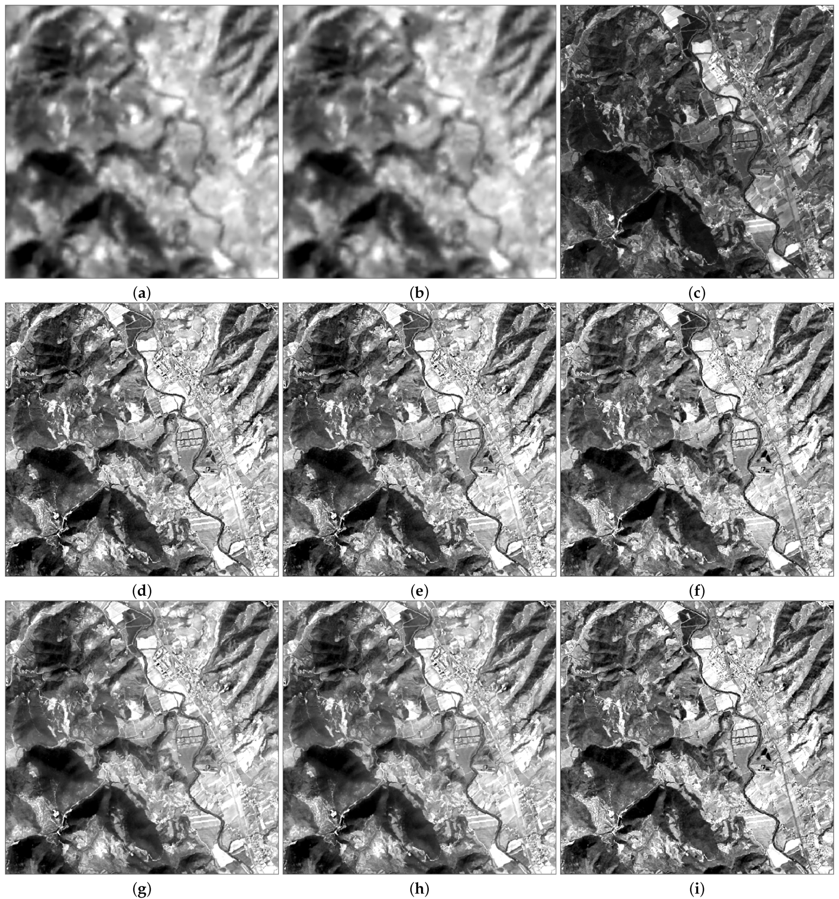
From the whole large scene, two sub-scenes, each of size 7.5 × 7.5 km2 have been cut: Scene 1 is a hilly vegetated region close to the Trasimeno Lake; Scene 2 is a built-up area crossed by the Tiber River, including part of the city of Perugia on the left and the vegetated hilly outskirts on the right. The thermal bands and the Pan images of the two scenes are displayed in Figure 6a–c and Figure 7a–c, respectively.
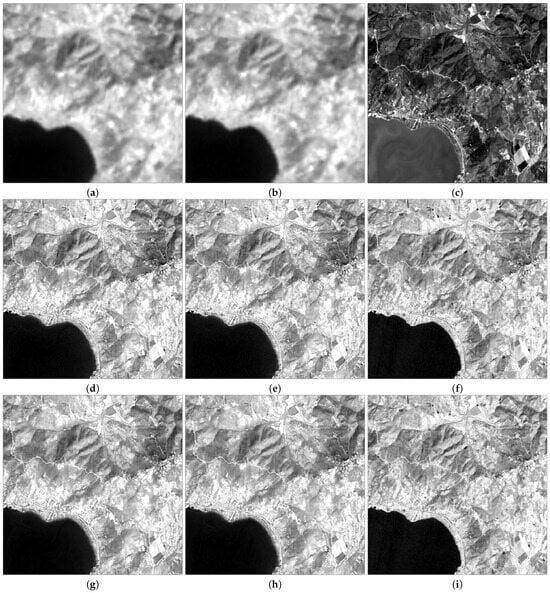
Figure 6.
Some 7.5 × 7.5 km2 details (500 × 500 pixels at 15 m spatial scale) of Scene 1 (lake and hilly area): (a) Interpolated original thermal band B10; (b) interpolated original thermal band B11; (c) original B8 (Pan); (d) B10 sharpened by B10-assimilated Pan; (e) B11 sharpened by B11-assimilated B8; (f) B10-assimilated B8; (g) B10 sharpened by original B8 (i.e., pansharpened B10); (h) B11 sharpened by original B8; (i) B11-assimilated B8.

Figure 7.
Some 7.5 × 7.5 km2 details (500 × 500 pixels at 15 m spatial scale) of Scene 2 (built-up and vegetated area): (a) Interpolated original thermal band B10; (b) interpolated original thermal band B11; (c) original B8 (Pan); (d) B10 sharpened by B10-assimilated Pan; (e) B11 sharpened by B11-assimilated B8; (f) B10-assimilated B8; (g) B10 sharpened by original B8 (i.e., pansharpened B10); (h) B11 sharpened by original B8; (i) B11-assimilated B8.
3.1. Analysis of Correlation
All statistical comparisons and fusion processes must be carried out with band formats different by a gain and an offset at most [43]. The optical data are expressed as surface reflectances, which is compatible with the surface radiance format of TIRS data converted from LST. Table 3 and Table 4 report the results of the LS solutions of the multivariate regressions in Equation (1) for the two TIRS bands, B10 and B11, carried out with the two subscenes. The extreme variability in weights is a consequence of the correlation among optical bands and of the presence of anomalous water pixels in Scene 1, anomalous because they affect the significance of statistics, not because they impair fusion. What immediately stands out is that , which roughly measures the correlation between the thermal band and the synthesized sharpening image, is considerably greater than the correlation of any individual band with TIR, reported in the last two rows of Table 2. The last two columns of Table 2 are unreliable due to the presence of the lake, which approximately behaves like a dark body in the wavelength intervals spanned by B5, B6, B7, and B9. On correlated spectral intervals, e.g., B1-B4, the spectral weights may have negative signs, possibly alternate. This would be surprising if the bands were uncorrelated, which is not true. Interestingly, the cirrus band B9 is not correlated with any of the other bands, including the thermal ones. This fact is concealed by the significant presence of pure water pixels in Scene 1 but stands out in Scene 2, where water pixels are mixed with land pixels. In fact, in Table 3 the weights of B9 are significantly nonzero; in Table 4, they are identically zero to the second digit included.
Table 3.
Scene 1: LS coefficients of the multivariate regressions of the VNIR bands that synthesize the 15 m sharpening bands of the two TIRS bands and related values of .
Table 4.
Scene 2: LS coefficients of the multivariate regressions of the VNIR bands that synthesize the 15 m sharpening bands of the two TIRS bands and related values of .
The most important result of this analysis is the following: in a reliable scene, without pure water pixels, attains values greater than 0.87 for both bands. In Scene 1, the presence of the lake artificially increases the correlation of the “dark” bands and raises to values up to 0.95. These values are greater than the values of CC of the original Pan image towards the TIRS bands, namely 0.665 and 0.671, averaged on the whole available scene. This result entails the use of the synthetic bands assimilated to the thermal bands to sharpen the TIRS bands according to the hypersharpening paradigm. The synthetic assimilated images are visible in Figure 6f,i and Figure 7f,i for Scene 1 and Scene 2, respectively.
3.2. Fusion Simulations
Figure 6d,e and Figure 7d,e portray the two TIRS bands B10 and B11 once they have been hypersharpened by means of the synthetic assimilated images in Figure 6f,i and Figure 7f,i, for the two sub-scenes. The fusion rule is the projection gain of Equation (3), with the synthetic Pan calculated as in Equation (2). Fusion of the TIRS bands is accomplished in surface radiance format and the fused bands are converted back to surface temperature for display, as in Figure 4, and modeling. Compared to the 100 m originals in Figure 6a,b and Figure 7a,b, the fused images are extremely detailed and finely textured; they look realistically enhanced, though nobody knows what the true 15 m images would look like.
Figure 6g,h and Figure 7g,h present the results of conventional pansharpening using only the 15 m Pan of OLI (B8), displayed in Figure 6c and Figure 7c. Although rather similar in appearance, the products of plain pansharpening are less enhanced and present less abrupt temperature edges.
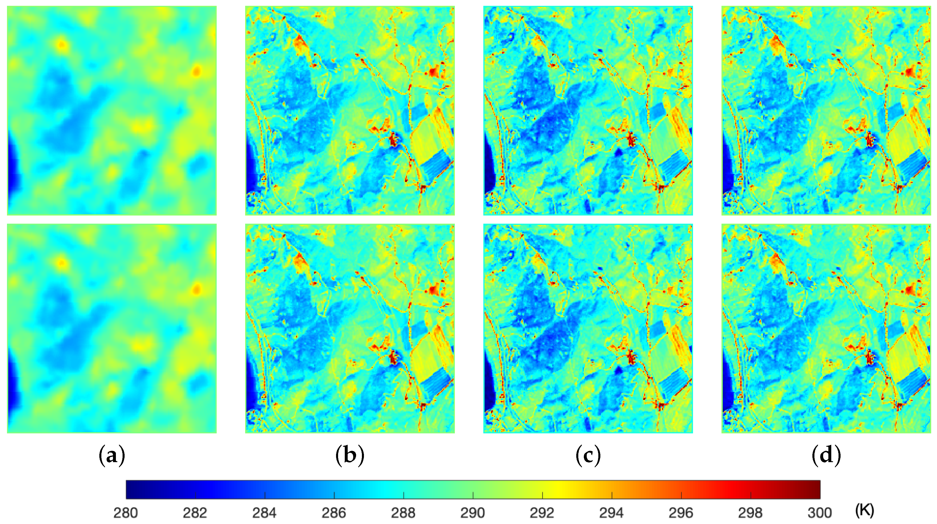
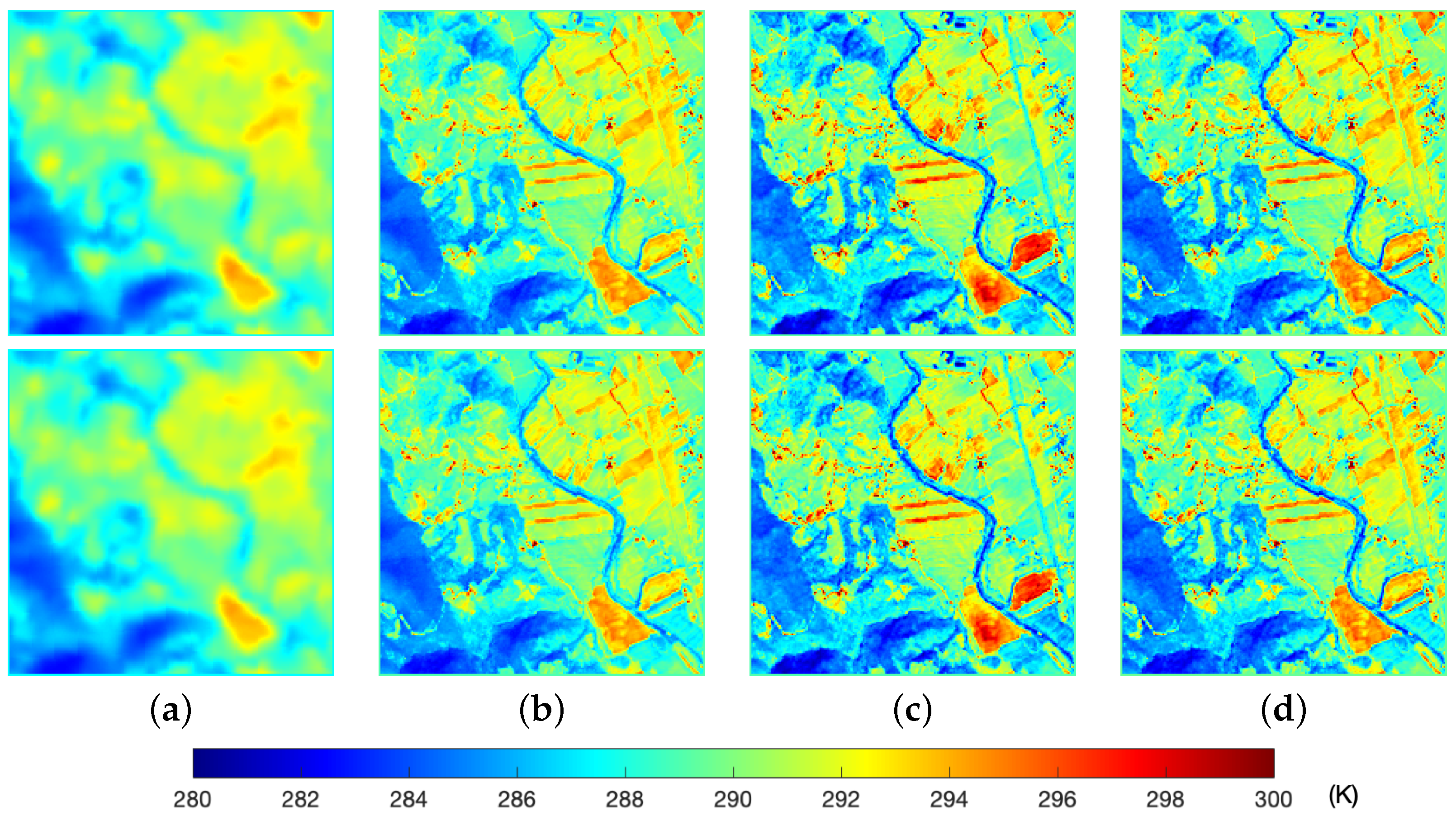
Fragments extracted from original and sharpened TIRS bands of the two subscenes have been converted back to absolute temperature and comparatively displayed with the associated color palette in Figure 8 and Figure 9. In Figure 8c, there are several clues that the assimilated thermal bands distort the thermal information: in the original (Figure 8a) the edge of the lake exhibits a gradual variation in temperature due to the increasing depth toward the center. This is clearly visible in both the sharpened images (Figure 8b,d) but not in the assimilated images, where the temperature jump is abrupt. Analogously, some patches in the assimilated image are colder or warmer than in the original and sharpened TIR bands. The geometry of the assimilated images is noteworthy, the radiometry, or thermal consistency towards the original, somewhat less. Instead, the sharpened images are geometrically and thermally accurate. In Figure 9, the superior thermal unmixing capability of the hypersharpened temperature map appears. The presence of the Tiber River is hardly recognized in the originals because the riverbed is narrower than the pixel size and water is mixed with vegetation or bare soil, having much lower thermal capacity than water. Thus, the pixel response is a mixture of water and side pixels. Both the sharpened images and the assimilated images are capable of unmixing the riverbed from its sides; the hypersharpened bands seem slightly more accurate because the assimilated image does not outline subtle temperature gradients across the riverbed. The biased response of the assimilated TIRS bands is noticeable in the lower right corners of the icons in Figure 9: the assimilated patches are up to 4 K warmer than the originals and 3 K warmer than the sharpened bands.

Figure 8.
Scene 1: 3 Km × 3 Km fragments (200 × 200 pixels at 15 m spatial scale) of original and sharpened thermal bands, B10 on upper row and B11 on lower row: (a) Interpolated original; (b) sharpened by original B8; (c) band-assimilated Pan; (d) sharpened by band-assimilated Pan.

Figure 9.
Scene 2: 3 Km × 3 Km fragments (200 × 200 pixels at 15 m spatial scale) of original and sharpened thermal bands, B10 on upper row and B11 on lower row: (a) Interpolated original; (b) sharpened by original B8; (c) band-assimilated Pan; (d) sharpened by band-assimilated Pan.
3.3. Statistical Evaluations
In addition to subjective evaluations, an objective quality analysis was carried out through no-reference statistical indexes that measure the consistency of fusion products with its components at the different scales: 100 m and 15 m.
Table 5 and Table 6 show that both pansharpening and hypersharpening preserve the original information, the proposed scheme, slightly better. Instead, the assimilation of the thermal bands from optical data, although highly popular in the literature [25,47], is almost 30% less accurate for what concerns the thermal consistency of the assimilated products compared to the originals.
Table 5.
Scene 1: thermal distortion index calculated between one enhanced TIRS band, spatially degraded to 100 m scale, and original 100 m TIRS. The index is expressed both as NRMSE% and as RMSE (K). Ideal case is 0.
Table 6.
Scene 2: thermal distortion index calculated between one enhanced TIRS band, spatially degraded to 100 m scale, and original 100 m TIRS. The index is expressed both as NRMSE% and as RMSE (K). Ideal case is 0.
Table 7 highlights that the proposed hypersharpening is better than conventional pansharpening in terms of spatial consistency. This is an immediate consequence of the fact that the low-spatial-frequency components of natural Pan (B8) are correlated with TIRS bands by about 67% on the non-water pixels (54% including the lake and the river). Conversely, the lower-frequency components of the TIRS-assimilated synthetic Pan are correlated over 87% with TIRS (over 94% including the lake). Correlation measurements are likely to be consistent across multiple scales. This explains why the synthetic Pan and not the natural Pan is the reference of spatial consistency. As a general remark, the spatial distortions reported for Scene 2 are twice those found for Scene 1 because the latter is much more textured and detailed than the former and hence more difficult to spatially enhance. The assimilated TIRS used for hypersharpening attain the ideal score of one, by definition. However, the price to be paid is the mediocre thermal consistency measured in Table 5 and Table 6. Instead, the original TIRS interpolated at 15 m provides the ideal scores of thermal consistency in Table 5 and Table 6, but here it exhibits less than mediocre spatial consistency, as one might expect.
Table 7.
Spatial distortion index [45] between thermal products and sharpening Pan, defined as average of the synthetic Pan’s assimilated to B10 and B11, respectively. The index ranges in [0, 1]. Ideal case is 0.
The radiometric and spatial consistency indexes can be coupled into a unique index, as it is usually done for assessment of MS pansharpening [46]. To do so, NRMSE, which ranges in [0, 1] should not be expressed in percentage. The cumulative consistency index can be defined as , where the thermal distortion, , is measured by NRMSE. We preferred to keep them separate, also because is measured from thermal data, from radiance data.
4. Discussion
At the end of the presentation of the results of downscaling of land surface temperature maps, a series of considerations can be made.
The synergy between assimilation and pansharpening performed by applying the hypersharpening paradigm seems to present advantages over both. The assimilation of the optical bands on the thermal bands exhibits unparalleled spatial detail, even if the spatial details might sometimes be incompatible with the nature of the thermal image. On the other hand, the multivariate regression is unable to correctly synthesize some homogeneous areas, where errors of a non-negligible entity are located.
Pansharpening alone has a good thermal consistency, in the sense that there are no visibly incorrect patches, good thermal unmixing capabilities, especially to be noted on the edge of the lake and along the river bed, and a good level of spatial sharpness, quite compatible with the nature of the thermal scene.
The proposed approach, which could be called “thermally assimilated hypersharpening”, balances the advantages and disadvantages of the methods that originate it: the thermal consistency is slightly higher than that of pansharpening, which was already considerably higher than that of direct assimilation; the thermal unmixing capacity is similar to pansharpening. The spatial detail is higher and at the same time quite plausible. The term plausible indicates that the true temperature map is unknown.
In some cases, one operates at a reduced scale, spatially degrading all the datasets of the same scale factor in order to use the thermal originals as a reference of the quality of the fusion. This strategy, widely used for unimodal fusion, may be questionable in the present case of a multimodal fusion, because at a larger scale the percentage of mixed pixels increases on spatially detailed scenes, such as urban areas, with the result that the specificity of the scene is lost. As the imaging scale gets finer. thermal images become contourless, because the temperature variable depicted does not have marked discontinuities due to heat diffusion.
In this sense, the evaluation of full-scale quality, in separate terms of thermal and geometric consistencies, seems more appropriate, also because in this way the real images are evaluated and with not low-resolution quicklooks. The methodology that followed, borrowed from optical data fusion, is also naturally suitable for multimodal fusion. It should be noted that downscaling procedures and consistency evaluations are based exclusively on widely established concepts of robust statistics and multiresolution analysis.
One limit of the proposed method would appear if the original thermal images attain metric resolution. Due to heat diffusion, high-resolution TIR images are almost “contourless” and the fused images would be unrealistically overenhanced. For satellite TIR images, the highest spatial resolution of an upcoming mission planned in 2028 is 60 m. This study pertains to the downscaling of LST maps, not to the sharpening of generic TIR imagery produced by thermal cameras in outdoor environments.
5. Conclusions
LandSat 8 was launched in 2013, followed in 2021 by LandSat 9. Both satellites were equipped with 30 m VNIR/SWIR MS scanners (OLI) and a two-band 100 m thermal scanner (TIRS). For continuity with the earlier ETM+ onboard LandSat 7, a 15 m Pan image was included in OLI, but its spectral coverage was limited to the interval (500–680) nm to expedite the sharpening of the TIRS bands, which are statistically uncorrelated from the radiance reflected by vegetation in the NIR wavelengths, 700 nm onward. This choice improves thermal pansharpening but slightly impairs the pansharpening of the NIR band. So far, TIR pansharpening of LandSat 8/9 data represents the state of the art for downscaling land temperature maps because the geometrical information of the 15 m Pan resolves the ambiguities of the 100 m TIRS data due to thermally mixed pixels containing objects of different temperatures.
In this study, we have shown that the relatively high scale ratio (100:15) for sharpening the TIRS bands through the optical bands benefits from the hypersharpening paradigm, which foresees as many sharpening images as there are TIRS bands, instead of the unique image of pansharpening. The high-resolution sharpening images are synthesized from all the 30 m optical bands of OLI and also from the 15 m Pan. Each of them is assimilated to a single TIRS band by means of a multivariate regression of the optical bands, the LS solution of which yields the best match to the original TIRS band. The advantage of the proposed hypersharpening is quantified by resorting to statistical consistency indexes, widespread for pansharpening.
Future developments will concern a possible object-based approach, in which the multivariate regression and the resulting assimilated synthetic Pan images are computed in statistically homogeneous segments [47]. Segmentation is trivially carried out on specific bands that are capable of discriminating different landscapes, e.g., water, vegetation, bare soil, and built-up areas. The sharpened TIRS bands will still be given by hypersharpening, which extracts the missing highpass information from the synthetic Pan images, assimilated to the different original TIRS bands. Another issue that may deserve attention concerns the assimilation procedure. Now, the color space is linearly mapped onto the thermal space by multivariate linear regression. The question is whether it is possible to obtain a better match by means of a nonlinear relationship. This has been found to produce slight improvements in the case of pansharpening [48], which is the fusion of homogeneous datasets. However, the inherent heterogeneity of thermal and optical data might be better captured by some nonlinear transformation of the optical space.
Author Contributions
Conceptualization, L.A. and A.G.; methodology, L.A. and A.G.; software, A.G.; validation, L.A. and A.G.; resources, L.A.; data curation, A.G.; writing—original draft preparation, L.A.; writing—review and editing, L.A. and A.G. All authors have read and agreed to the published version of the manuscript.
Funding
This research received no external funding.
Data Availability Statement
Publicly available datasets were analyzed in this study. The image data can be freely downloaded from https://earthexplorer.usgs.gov (accessed on 20 October 2024).
Acknowledgments
The authors are indebted to their former coauthor A. Arienzo, with whom this study was initiated.
Conflicts of Interest
The authors declare no conflicts of interest.
References
- Li, Z.L.; Tang, B.H.; Wu, H.; Ren, H.; Yan, G.; Wan, Z.; Trigo, I.F.; Sobrino, J.A. Satellite-derived land surface temperature: Current status and perspectives. Remote Sens. Environ. 2013, 131, 14–37. [Google Scholar] [CrossRef]
- Sandholt, I.; Rasmussen, K.; Andersen, J. A simple interpretation of the surface temperature/vegetation index space for assessment of surface moisture status. Remote Sens. Environ. 2002, 79, 213–224. [Google Scholar] [CrossRef]
- Eckmann, T.C.; Roberts, D.A.; Still, C.J. Using multiple endmember spectral mixture analysis to retrieve subpixel fire properties from MODIS. Remote Sens. Environ. 2008, 112, 3773–3783. [Google Scholar] [CrossRef]
- Voogt, J.; Oke, T. Thermal remote sensing of urban climates. Remote Sens. Environ. 2003, 86, 370–384. [Google Scholar] [CrossRef]
- Crow, W.T.; Wood, E.F. The assimilation of remotely sensed soil brightness temperature imagery into a land surface model using Ensemble Kalman filtering: A case study based on ESTAR measurements during SGP97. Adv. Water Res. 2003, 26, 137–149. [Google Scholar] [CrossRef]
- Kustas, W.; Anderson, M. Advances in thermal infrared remote sensing for land surface modeling. Agricult. For. Meteor. 2009, 149, 2071–2081. [Google Scholar] [CrossRef]
- Santarelli, C.; Carfagni, M.; Alparone, L.; Arienzo, A.; Argenti, F. Multimodal fusion of tomographic sequences of medical images: MRE spatially enhanced by MRI. Comput. Meth. Programs Biomed. 2022, 223, 106964. [Google Scholar] [CrossRef]
- Aiazzi, B.; Alparone, L.; Baronti, S.; Santurri, L.; Selva, M. Spatial resolution enhancement of ASTER thermal bands. In Proceedings of the Image and Signal Processing for Remote Sensing XI, Bruges, Belgium, 20–22 September 2005; Bruzzone, L., Ed.; Proceedings of SPIE. SPIE: Bellingham, WA, USA, 2005; Volume 5982, p. 59821G. [Google Scholar] [CrossRef]
- Rodriguez-Galiano, V.; Pardo-Iguzquiza, E.; Sanchez-Castillo, M.; Chica-Olmo, M.; Chica-Rivas, M. Downscaling Landsat 7 ETM+ thermal imagery using land surface temperature and NDVI images. Int. J. Appl. Earth Observ. Geoinform. 2012, 18, 515–527. [Google Scholar] [CrossRef]
- Garzelli, A.; Aiazzi, B.; Alparone, L.; Lolli, S.; Vivone, G. Multispectral pansharpening with radiative transfer-based detail-injection modeling for preserving changes in vegetation cover. Remote Sens. 2018, 10, 1308. [Google Scholar] [CrossRef]
- Kustas, W.P.; Norman, J.M.; Anderson, M.C.; French, A.N. Estimating subpixel surface temperatures and energy fluxes from the vegetation index–radiometric temperature relationship. Remote Sens. Environ. 2003, 85, 429–440. [Google Scholar] [CrossRef]
- Agam, N.; Kustas, W.P.; Anderson, M.C.; Li, F.; Neale, C.M.U. A vegetation index based technique for spatial sharpening of thermal imagery. Remote Sens. Environ. 2007, 107, 545–558. [Google Scholar] [CrossRef]
- Jeganathan, C.; Hamm, N.A.S.; Mukherjee, S.; Atkinson, P.M.; Raju, P.L.N.; Dadhwal, V.K. Evaluating a thermal image sharpening model over a mixed agricultural landscape in India. Int. J. Appl. Earth Observ. Geoinform. 2011, 13, 178–191. [Google Scholar] [CrossRef]
- Chen, X.; Yamaguchi, Y.; Chen, J.; Shi, Y. Scale effect of vegetation-index-based spatial sharpening for thermal imagery: A simulation study by ASTER data. IEEE Geosci. Remote Sens. Lett. 2012, 9, 549–553. [Google Scholar] [CrossRef]
- Dominguez, A.; Kleissl, J.; Luvall, J.C.; Rickman, D.L. High-resolution urban thermal sharpener (HUTS). Remote Sens. Environ. 2011, 115, 1772–1780. [Google Scholar] [CrossRef]
- Zhan, W.; Chen, Y.; Zhou, J.; Wang, J.; Liu, W.; Voogt, J.; Zhu, X.; Quan, J.; Li, J. Disaggregation of remotely sensed land surface temperature: Literature survey, taxonomy, issues, and caveats. Remote Sens. Environ. 2013, 131, 119–139. [Google Scholar] [CrossRef]
- Huryna, H.; Cohen, Y.; Karnieli, A.; Panov, N.; Kustas, W.P.; Agam, N. Evaluation of TsHARP utility for thermal sharpening of Sentinel-3 satellite images using Sentinel-2 visual imagery. Remote Sens. 2019, 11, 2304. [Google Scholar] [CrossRef]
- Wang, J.; Schmitz, O.; Lu, M.; Karssenberg, D. Thermal unmixing based downscaling for fine resolution diurnal land surface temperature analysis. ISPRS J. Photogramm. Remote Sens. 2020, 161, 76–89. [Google Scholar] [CrossRef]
- Garrigues, S.; Allard, D.; Baret, F.; Weiss, M. Quantifying spatial heterogeneity at the landscape scale using variogram models. Remote Sens. Environ. 2006, 103, 81–96. [Google Scholar] [CrossRef]
- Wang, J.W.; Chow, W.T.; Wang, Y.C. A global regression method for thermal sharpening of urban land surface temperatures from MODIS and Landsat. Int. J. Remote Sens. 2020, 41, 2986–3009. [Google Scholar] [CrossRef]
- McCabe, M.F.; Balik, L.K.; Theiler, J.; Gillespie, A.R. Linear mixing in thermal infrared temperature retrieval. Int. J. Remote Sens. 2008, 29, 5047–5061. [Google Scholar] [CrossRef]
- Firozjaei, M.K.; Kiavarz, M.; Alavipanah, S.K. Satellite-derived land surface temperature spatial sharpening: A comprehensive review on current status and perspectives. Eur. J. Remote Sens. 2022, 55, 644–664. [Google Scholar] [CrossRef]
- Selva, M.; Aiazzi, B.; Butera, F.; Chiarantini, L.; Baronti, S. Hyper-sharpening: A first approach on SIM-GA data. IEEE J. Sel. Top. Appl. Earth Observ. Remote Sens. 2015, 8, 3008–3024. [Google Scholar] [CrossRef]
- Fasbender, D.; Tuia, D.; Bogaert, P.; Kanevski, M. Support-based implementation of Bayesian data fusion for spatial enhancement: Applications to ASTER thermal images. IEEE Geosci. Remote Sens. Lett. 2008, 5, 598–602. [Google Scholar] [CrossRef]
- Zhan, W.; Chen, Y.; Zhou, J.; Li, J.; Liu, W. Sharpening thermal imageries: A generalized theoretical framework from an assimilation perspective. IEEE Trans. Geosci. Remote Sens. 2011, 49, 773–789. [Google Scholar] [CrossRef]
- Addesso, P.; Longo, M.; Restaino, R.; Vivone, G. Sequential Bayesian methods for resolution enhancement of TIR image sequences. IEEE J. Sel. Top. Appl. Earth Observ. Remote Sens. 2015, 8, 233–243. [Google Scholar] [CrossRef]
- Alparone, L.; Arienzo, A.; Garzelli, A. Spatial resolution enhancement of satellite hyperspectral data via nested hypersharpening with Sentinel-2 multispectral data. IEEE J. Sel. Top. Appl. Earth Observ. Remote Sens. 2024, 17, 10956–10966. [Google Scholar] [CrossRef]
- Guo, S.; Li, M.; Li, Y.; Chen, J.; Zhang, H.K.; Sun, L.; Wang, J.; Wang, R.; Yang, Y. The improved U-STFM: A deep learning-based nonlinear spatial-temporal fusion model for land surface semperature downscaling. Remote Sens. 2024, 16, 322. [Google Scholar] [CrossRef]
- Ma, J.; Yu, W.; Liang, P.; Li, C.; Jiang, J. FusionGAN: A generative adversarial network for infrared and visible image fusion. Inform. Fusion 2019, 48, 11–26. [Google Scholar] [CrossRef]
- Abady, L.; Barni, M.; Garzelli, A.; Tondi, B. GAN generation of synthetic multispectral satellite images. In Proceedings of the Image and Signal Processing for Remote Sensing XXVI, Online, 21–25 September 2020; Bruzzone, L., Ed.; Proceedings of SPIE. SPIE: Bellingham, WA, USA, 2020; Volume 11533, p. 115330. [Google Scholar] [CrossRef]
- Aiazzi, B.; Alparone, L.; Baronti, S.; Lastri, C. Crisp and fuzzy adaptive spectral predictions for lossless and near-lossless compression of hyperspectral imagery. IEEE Geosci. Remote Sens. Lett. 2007, 4, 532–536. [Google Scholar] [CrossRef]
- Aiazzi, B.; Alparone, L.; Baronti, S.; Pippi, I.; Selva, M. Generalised Laplacian pyramid-based fusion of MS + P image data with spectral distortion minimisation. In Proceedings of the PCV 2002, Graz, Austria, 9–13 September 2002; ISPRS Archives. Volume 34, pp. 1–4. [Google Scholar]
- Aiazzi, B.; Alparone, L.; Baronti, S.; Garzelli, A.; Selva, M. Advantages of Laplacian pyramids over “à trous” wavelet transforms for pansharpening of multispectral images. In Proceedings of the Image and Signal Processing for Remote Sensing XVIII, Edinburgh, UK, 24–26 September 2012; Bruzzone, L., Ed.; Proceedings of SPIE. SPIE: Bellingham, WA, USA, 2012; Volume 8537, pp. 12–21. [Google Scholar] [CrossRef]
- Aiazzi, B.; Baronti, S.; Selva, M.; Alparone, L. Enhanced Gram-Schmidt spectral sharpening based on multivariate regression of MS and Pan data. In Proceedings of the 2006 IEEE International Geoscience and Remote Sensing Symposium (IGARSS), Denver, CO, USA, 31 July–4 August 2006; pp. 3806–3809. [Google Scholar] [CrossRef]
- Garzelli, A.; Nencini, F. Fusion of panchromatic and multispectral images by genetic algorithms. In Proceedings of the 2006 IEEE International Geoscience and Remote Sensing Symposium (IGARSS), Denver, CO, USA, 31 July–4 August 2006; pp. 3810–3813. [Google Scholar] [CrossRef]
- Aiazzi, B.; Baronti, S.; Lotti, F.; Selva, M. A comparison between global and context-adaptive pansharpening of multispectral images. IEEE Geosci. Remote Sens. Lett. 2009, 6, 302–306. [Google Scholar] [CrossRef]
- Selva, M.; Santurri, L.; Baronti, S. Improving hypersharpening for WorldView-3 data. IEEE Geosci. Remote Sens. Lett. 2019, 16, 987–991. [Google Scholar] [CrossRef]
- Aiazzi, B.; Alparone, L.; Argenti, F.; Baronti, S. Wavelet and pyramid techniques for multisensor data fusion: A performance comparison varying with scale ratios. In Proceedings of the Image and Signal Processing for Remote Sensing V, Florence, Italy, 22–24 September 1999; Serpico, S.B., Ed.; SPIE: Bellingham, WA, USA, 1999. Proceedings of SPIE. Volume 3871, pp. 251–262. [Google Scholar] [CrossRef]
- Garzelli, A.; Nencini, F.; Alparone, L.; Baronti, S. Multiresolution fusion of multispectral and panchromatic images through the curvelet transform. In Proceedings of the 2005 IEEE International Geoscience and Remote Sensing Symposium (IGARSS), Seoul, Republic of Korea, 29–29 July 2005; pp. 2838–2841. [Google Scholar] [CrossRef]
- Aiazzi, B.; Alparone, L.; Baronti, S.; Carlà, R.; Garzelli, A.; Santurri, L. Sensitivity of pansharpening methods to temporal and instrumental changes between multispectral and panchromatic data sets. IEEE Trans. Geosci. Remote Sens. 2017, 55, 308–319. [Google Scholar] [CrossRef]
- Restaino, R.; Vivone, G.; Addesso, P.; Chanussot, J. Hyperspectral sharpening approaches using satellite multiplatform data. IEEE Trans. Geosci. Remote Sens. 2021, 59, 578–596. [Google Scholar] [CrossRef]
- Alparone, L.; Garzelli, A.; Vivone, G. Intersensor statistical matching for pansharpening: Theoretical issues and practical solutions. IEEE Trans. Geosci. Remote Sens. 2017, 55, 4682–4695. [Google Scholar] [CrossRef]
- Arienzo, A.; Aiazzi, B.; Alparone, L.; Garzelli, A. Reproducibility of pansharpening methods and quality indexes versus data formats. Remote Sens. 2021, 13, 4399. [Google Scholar] [CrossRef]
- Aiazzi, B.; Alparone, L.; Baronti, S.; Carlà, R. Assessment of pyramid-based multisensor image data fusion. In Proceedings of the Image and Signal Processing for Remote Sensing IV, Barcelona, Spain, 21–25 September 1998; Serpico, S.B., Ed.; SPIE: Bellingham, WA, USA, 1998. Proceedings of SPIE. Volume 3500, pp. 237–248. [Google Scholar] [CrossRef]
- Alparone, L.; Garzelli, A.; Vivone, G. Spatial consistency for full-scale assessment of pansharpening. In Proceedings of the 2018 IEEE International Geoscience and Remote Sensing Symposium (IGARSS), Valencia, Spain, 22–27 July 2018; pp. 5132–5134. [Google Scholar] [CrossRef]
- Arienzo, A.; Vivone, G.; Garzelli, A.; Alparone, L.; Chanussot, J. Full-resolution quality assessment of pansharpening: Theoretical and hands-on approaches. IEEE Geosci. Remote Sens. Mag. 2022, 10, 2–35. [Google Scholar] [CrossRef]
- Xia, H.; Chen, Y.; Quan, J.; Li, J. Object-based window strategy in thermal sharpening. Remote Sens. 2019, 11, 634. [Google Scholar] [CrossRef]
- Arienzo, A.; Alparone, L.; Garzelli, A.; Lolli, S. Advantages of nonlinear intensity components for contrast-based multispectral pansharpening. Remote Sens. 2022, 14, 3301. [Google Scholar] [CrossRef]


Disclaimer/Publisher’s Note: The statements, opinions and data contained in all publications are solely those of the individual author(s) and contributor(s) and not of MDPI and/or the editor(s). MDPI and/or the editor(s) disclaim responsibility for any injury to people or property resulting from any ideas, methods, instructions or products referred to in the content. |
© 2024 by the authors. Licensee MDPI, Basel, Switzerland. This article is an open access article distributed under the terms and conditions of the Creative Commons Attribution (CC BY) license (https://creativecommons.org/licenses/by/4.0/).