Abstract
The effectiveness of supervised ML heavily depends on having a large, accurate, and diverse annotated dataset, which poses a challenge in applying ML for yield prediction. To address this issue, we developed a self-training random forest algorithm capable of automatically expanding the annotated dataset. Specifically, we trained a random forest regressor model using a small amount of annotated data. This model was then utilized to generate new annotations, thereby automatically extending the training dataset through self-training. Our experiments involved collecting data from over 30 winter wheat varieties during the 2019–2020 and 2021–2022 growing seasons. The testing results indicated that our model achieved an R2 of 0.84, RMSE of 627.94 kg/ha, and MAE of 516.94 kg/ha in the test dataset, while the validation dataset yielded an R2 of 0.81, RMSE of 692.96 kg/ha, and MAE of 550.62 kg/ha. In comparison, the standard random forest resulted in an R2 of 0.81, RMSE of 681.02 kg/ha, and MAE of 568.97 kg/ha in the test dataset, with validation results of an R2 of 0.79, RMSE of 736.24 kg/ha, and MAE of 585.85 kg/ha. Overall, these results demonstrate that our self-training random forest algorithm is a practical and effective solution for expanding annotated datasets, thereby enhancing the prediction accuracy of ML models in winter wheat yield forecasting.
1. Introduction
Wheat is one of the most important and indispensable staple cereal crops worldwide, of which 80% is winter wheat. China is one of the major winter-wheat growing countries [1]. Due to the impact of the food crisis and global climate change, precise prediction of wheat yield is of great significance. Globally, estimating crop yield is one of the most critical issues that policy and decision makers need to consider for assessing annual crop productivity and food supply [2].
Nowadays, in the field of agricultural applications, unmanned aerial vehicles (UAVs) and satellite multispectral remote sensing technology have become important techniques for crop growth monitoring and yield prediction. By comprehensively considering the multispectral information and data collection period of vegetation, important technical support can be provided for crop yield estimation and growth assessment at different scales. Satellite remote sensing and a geographic information system (GIS) could enable the estimation of crop production parameters over large geographic areas [2,3,4,5,6,7]. UAV-based platforms are capable of collecting large amounts of high-dimensional spectral data in a short period, which could be leveraged to evaluate the overall growth of wheat and predict wheat yield accurately [8,9,10,11].
In recent years, machine learning (ML) and deep learning (DL) methods have attracted attention in wheat yield prediction due to their high prediction accuracy in various applications. Using machine learning (ML) techniques for the fusion of UAV-based multi-sensor data can improve the prediction accuracy of wheat yield [10]. Random forest regression (RFR) has been leveraged to build regional- and local-scale yield prediction models at the pixel level for three southeast Australian wheat-growing paddocks [11]. Convolutional neural network (CNN) models have been employed to predict the yield of winter wheat, achieving significant improvements compared to linear regression models based on enhanced vegetation index 2 (EVI2) [12]. The results suggested that a CNN had the potential to enhance the accuracy of yield prediction. Various ML algorithms (such as ridge and lasso regression, classification and regression trees, k-nearest neighbor, support vector machines, gradient boosting, extreme gradient boosting, and random forest) have been used for wheat yield prediction to analyze the variability in wheat yield from farms in the northwestern Indo-Gangetic Plains of India. The findings indicated that tree-based and decision boundary-based models outperformed regression-based models in explaining wheat yield variability, with the random forest model emerging as the best-performing method in terms of goodness-of-fit and model precision and accuracy in wheat yield prediction, as measured by RMSE, MAE, and R2 [13].
The methods discussed are primarily based on supervised learning, known for their high prediction accuracy. However, the effectiveness of supervised machine learning (ML) algorithms relies on the availability of a substantial volume of accurate and diverse annotated data. Furthermore, it is crucial that the annotated data remains relatively balanced across different categories. If there is an imbalance or insufficient data for any particular type, supervised ML algorithms may become prone to overfitting on specific annotated features, leading to diminished performance in accurately predicting outcomes.
The high cost of the data annotation process presents a challenge for many tasks, making it difficult to obtain strong supervisory information, such as all-real labels [14]. The key contribution of this article lies in the combination of both advantages: utilizing a small amount of labeled data and improving the accuracy of winter wheat yield predictions. To this end, this article proposes a self-training random forest semi-supervised algorithm for yield prediction. In the experiments, we utilize the multispectral reflectance and water stress index of wheat obtained by a drone equipped with a multispectral camera, alongside a small amount of labeled yield data. The unlabeled wheat multispectral data are annotated to expand the training set, and the newly generated training set is employed for yield prediction.
Considering the multi-month growth cycle of winter wheat, which is easily influenced by natural conditions such as weather and diseases, we select the filling stage prior to maturity for yield prediction. The contributions of this study are as follows:
- (1)
- Our proposed solution achieves large-scale yield prediction based on ML with a small amount of ground data annotation. It provides a new perspective on the relationship between multispectral reflectance information and winter wheat yield;
- (2)
- Our solution offers a more efficient, time-saving, and labor-saving approach to expanding annotated datasets.
2. Materials and Methods
2.1. Research Location and Experiments Design
The testing data were collected from the Xinxiang Experimental Base of the Institute of Farmland Irrigation, part of the Chinese Academy of Agricultural Sciences, located in Henan Province, China, at the coordinates 35.20°N and 113.80°E. This area experiences an average annual temperature of about 14 °C and receives approximately 573.4 mm of rainfall annually, making it suitable for winter wheat cultivation. The dataset includes winter wheat yield information from two sampling areas (Test Field I and Test Field II) for the years 2020 and 2022, respectively. Each sampling area consists of a total of 180 test plots, with each plot measuring 8 m in length and 1.4 m in width.
In Test Field I during the 2019–2020 growing season, winter wheat was subjected to three different moisture levels: W1 (240 mm), W2 (190 mm), and W3 (145 mm). Within the field, each irrigation treatment involved 60 plots, corresponding to 30 different wheat varieties, and each of them was replicated twice. The water treatments were applied six times during various growth stages: the tillering stage, overwintering stage, turning green stage, jointing stage, heading stage, and filling stage, as outlined in Table 1.

Table 1.
An overview of the water treatment within the 2019–2020 growing season.
During the 2021–2022 growing season, winter wheat was subjected to six different irrigation levels: I1 (282 mm), I2 (254 mm), I3 (198 mm), I4 (141 mm), I5 (85 mm), and I6 (0 mm). Each treatment consisted of 30 plots, and 10 wheat varieties were selected for this study. Water treatments were applied four times, specifically at the overwintering stage, jointing stage, heading stage, and filling stage, as detailed in Table 2.

Table 2.
An overview of the water treatment within the 2021–2022 growing season.
In Test Field II within the 2021–2022 growing season, the 180 test plots were organized into six levels of nitrogen fertilizer application. Each treatment comprised 30 plots, with 10 different wheat varieties planted in each. The nitrogen fertilization treatments were applied twice, specifically at the jointing stage and the heading stage, as shown in Table 3.

Table 3.
An overview of the N fertilization treatment within the 2021–2022 growing season.
We conducted our analysis in 2020 for Test Field I and in 2022 for both Test Fields I and II. During the 2020–2021 growing season, we performed water stress experiments on winter wheat with varying irrigation amounts in Test Field I. However, due to heavy rainfall in Henan Province in 2021, the experiment was compromised, and the data lost their relevance. All winter wheat was sown between mid-October and early November of the previous year, with harvesting taking place in June of the following year, marking the end of the growing season.
In the wheat planting experiments conducted in 2020 and 2022, only a few winter wheat varieties overlapped. In the 2020 experiment, there were 30 winter wheat varieties, which included both disease-resistant and disease-susceptible varieties. These comprised winter wheat varieties suitable for cultivation in Henan Province, as well as those suitable for the Guanzhong Plain and the northern North China Plain. In contrast, all the winter wheat varieties used in the 2022 experiment were disease-resistant and suited for cultivation in Henan Province and its surrounding areas.
2.2. Weather Variability in Winter Wheat Growth
To ensure the smooth overwintering of wheat and to prevent it from freezing to death, all winter wheat was adequately watered before entering the overwintering period (early December). Winter wheat growing in the fields inevitably encountered varying weather changes throughout this period. Table 4 presents the weather profile for two seasons of winter wheat, spanning from the onset of the overwintering period to the maturity stage. This profile includes data on daily average temperature, humidity, and monthly precipitation.

Table 4.
An overview of the weather within the growing seasons.
From Table 4, it is evident that during the two winter wheat experiments conducted in different years, the average daily temperature reached its lowest point in January and its highest point in May. However, there were variations in the average daily temperatures for the same month across different years. The average daily humidity did not show a clear relationship with seasons or months, and there were significant differences between the two winter wheat experiments.
In the 2019–2020 wheat growth experiment, the highest recorded daily average humidity was 90%, occurring in December 2019. In contrast, during the 2021–2022 wheat experiment, the peak daily average humidity of 87.28% was observed in January 2022.
There were also notable differences in monthly precipitation between the two winter wheat growth experiments. In the 2019–2020 winter wheat experiment, precipitation was relatively consistent, with a maximum monthly total of 83.7 mm in May 2020 and a minimum of 4.4 mm in March 2020. During the 2021–2022 winter wheat growth period, maximum precipitation reached 109.3 mm in May, while no precipitation was recorded in February.
2.3. Data Acquisition
Data collection included UAV remote sensing images and field sampling, conducted according to different growth periods, fertilization treatment, and irrigation levels. Field data sampling occurred simultaneously with the flight periods.
2.3.1. Ground Truth Data
Crop yield was measured across the entire research area one day after the winter wheat maturation period began. In 2020, it was 2 June, and in 2022, it was 8 June. The harvested wheat from each plot was placed in a numbered bag and dried in the laboratory until a constant weight was achieved. The wheat from each plot was then weighed, and yield was calculated based on the plot area.
2.3.2. UAV-Based Data
For data collection, UAV flight tests were performed during the winter wheat filling stage on 10 May 2020 and 6 May 2022. Flights were conducted under clear conditions and during optimal lighting hours (10:00 a.m. to 2:00 p.m. Beijing time). Canopy spectral data from all plots were collected using a Rededge MX multispectral camera (Micasense, Inc., Seattle, WA, USA) and a Zenmuse XT2 thermal infrared camera (DJI Technology Co., Ltd., Shenzhen, China) mounted on Dji M210 quadrotor UAV (DJI Technology Co., Ltd., Shenzhen, China) (Figure 1).
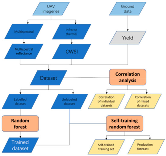
Figure 1.
Methodological flowchart for crop yield prediction from the unmanned aerial vehicle (UAV) imageries in combination with ground-based data.
Two remote sensing datasets—multispectral and thermal infrared—were acquired during the filling stages of 2020 and 2022. The multispectral images included spectral channels in five distinct wavelengths: blue (475 nm), green (560 nm), red (668 nm), red edge (717 nm), and near-infrared (840 nm). Each channel had specific bandwidths: the blue and green channels had bandwidths of 20 nm, while the red and red edge channels had narrower bandwidths of 10 nm. The near-infrared channel had a broader bandwidth of 40 nm. Thermal infrared images were obtained with a resolution of 640 × 512 pixels, covering a wavelength range of 7.5–13.5 μm.
Eighteen ground control points (GCPs) were established throughout the experimental field, using black and white boards evenly distributed across 180 plots. Canopy spectral images were captured through a 2D route planning flight mode, wherein the camera was configured to take images vertically relative to the ground at specified time intervals. The flight route was meticulously planned using 2D orthographic images obtained from DJI’s GPS ground station. The flight operation achieved a lateral overlap rate of 80% and a heading overlap rate of 85%, which are critical for ensuring high-quality image stitching and accurate data collection. The flight was conducted at an altitude of 40 m, allowing for suitable coverage and detail in the captured spectral imagery.
The photogrammetric processing of the acquired UAV images was performed using Pix4Dmapper v4.4.12 software (Pix4D S.A., Lausanne, Switzerland). Following the aerial triangulation of the UAV images, the geometric processing was optimized by incorporating the coordinates of the ground control points (GCPs). For the multispectral data, radiometric calibration was conducted using MicaSense calibrated reference panels, which have known reflectance values (MicaSense, Seattle, WA, USA). These panels were used to convert the raw image digital numbers (DNs) into calibrated reflectance values, with measurements taken immediately before and after each flight. Additionally, the sensor’s sensitivity to light, indicated by ISO values recorded by the downwelling light sensor, was utilized to support the radiometric calibration. Both the RGB and multispectral datasets were then converted to GeoTIFF format, employing the projected geographic coordinate system WGS 1984 UTM Zone 31N.
Figure 1 illustrates the methodological flowchart for this paper. After data processing, the correlation between multispectral information and winter wheat yield was analyzed. A classical random forest model was then employed to train an initial regressor. Following this, a self-training random forest algorithm was utilized to expand the training set and perform the yield prediction.
2.4. Selection of Spectral Information
In this research, by using a multispectral camera, the reflectance of red light (), green light (), blue light (), red edge (), and near-infrared () of wheat during the filling period were collected.
To learn more about winter wheat, we utilized a thermal infrared multispectral camera to enhance our collection of multispectral data. This thermal infrared camera captured the temperature characteristics of the winter wheat canopy. Canopy temperature results from complex energy exchanges within agricultural ecosystems and is influenced by various external factors. In this study, we collected the crop water stress index (CWSI), which was used to eliminate sensitivity to surrounding environmental conditions (such as air temperature, humidity, and radiation) and standardize the measured canopy temperature, as the thermal infrared information of winter wheat, as shown in Equation (1).
This is obtained using the simplified water stress index CWSI defined by Jones [15] and the infrared characteristics of winter wheat canopy experiments, where was the average temperature of the canopy of one plot, was the highest temperature of the canopy of the plot, and was the lowest temperature of the canopy of the plot.
2.5. Pseudo Label Generation
Self-training belongs to the semi-supervised branch of machine learning algorithms because it trains models using a combination of labeled and unlabeled data. The core idea is to first train a weak regressor with a small amount of annotated data and then use this weak regressor to predict unlabeled samples. When certain conditions are met, the predicted result is used as the true label of the sample. Then, the model is trained again with the existing annotated data, and the unlabeled samples are annotated and iterated repeatedly. Finally, it ends when the stop condition is reached.
The biggest problem with self-training algorithms is that incorrect pseudo labels introduce too much noise, which can mislead the model’s training. Some research [16] has found that it is feasible to exploit the uncertainty estimation of the underlying neural network to improve the self-training mechanism. For each unlabeled data point selected, it was passed into an NN (neural network) several times. Because dropout was used, they obtained uncertainty prediction results. Directly averaging the predictions results in the obtainment of the prediction label.
In this study, we moved away from the conventional neural network approach and instead employed a random forest regression model for assigning pseudo labels. The random forest method utilized bootstrapping, which involved sampling with replacement to create new training sets from the original data. Each training set was formed by randomly selecting (n) samples.
For every new training set created, multiple sub-models were trained. The predictions from these individual models were then averaged to generate the pseudo labels. This averaging process effectively exploited the inherent uncertainty within the training data, which enhanced the reliability of the pseudo labels and helped reduce the negative impact of noise in the dataset.
2.6. Multi-Scale Joint Prediction
During the self-training process, samples with high-confidence predictions are more likely to be accurately labeled. However, if these predictions are incorrect, it can lead to mislabeling, which is a challenge since these mislabeled samples are often difficult to predict correctly, distorting the data distribution.
In this paper, after obtaining pseudo-labels using random forest regression, a multi-scale joint prediction approach was employed. Within this framework, trusted pseudo-labels were selectively identified, and data associated with these trusted labels were incorporated into the training set, constituting the self-training process.
Firstly, the entire unlabeled dataset ‘e’ was uniformly divided into three subsets: ‘b’, ‘c’, and ‘d’. Specifically, the data in ‘a’ representing a plot (illustrated in Figure 2) were selected, which belong to the red segment. This dataset ‘a’ underwent five predictions, based on five distinct training sets constructed by combining the original training set with the pseudo-labeled datasets ‘a’, ‘b’, ‘c’, ‘d’, and ‘e’, respectively.

Figure 2.
Multi-scale joint prediction.
Secondly, pseudo labels were considered trustworthy if the absolute difference between their predicted values and the assigned pseudo labels fell below a predetermined threshold (δ), which was determined through iterative experimentation.
2.7. Self-Training Random Forest Architecture
In this paper, we focused on predicting winter wheat yield and aimed to achieve highly reliable wheat yield forecasts through two processes: (i) training a regressor using a small amount of labeled data and (ii) annotating the data in the unlabeled dataset using a self-training random forest regressor to expand the training set.
Two critical issues were identified. The first issue involved selecting an appropriate regression model and a small, annotated dataset with comprehensive information to generate trustworthy pseudo labels. Our approach was to use the random forest algorithm to reduce the impact of noise. The second issue was to increase the prediction accuracy of high-confidence samples included in the unlabeled datasets.
Figure 3 illustrated the training process of the self-training random forest algorithm, which involved training the initial random forest model, employing a multi-scale joint prediction method for self-training, labeling unlabeled data, and selecting trustworthy pseudo-labeled data to expand the training set. The specific process was as follows:
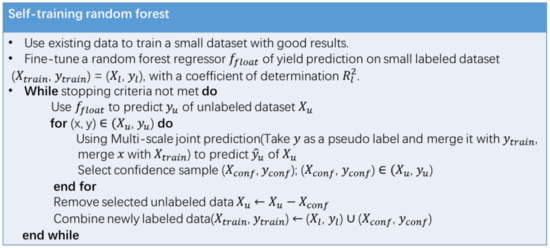
Figure 3.
Pseudo code of self-training random forest.
- A random forest regressor, , was trained for winter wheat prediction and calculating pseudo labels for unlabeled samples;
- Then, the training set (, ) was concatenated with unlabeled samples that had pseudo labels, creating a temporary training set (, ). This set was used to select confidence samples (, ) to add to the original training set using multi-scale joint prediction method;
- Confidence samples were removed from the unlabeled dataset, and the previous step was repeated until the stopping criteria were met;
- Finally, predictions were made for winter wheat using the newly trained random forest network based on the expanded training set.
Table 5 presents the relevant parameters that were considered. The n_estimators represent the number of trees in the random forest regressor. The min_samples_leaf represents minimum samples size on leaf nodes. The random forest regressor was trained using sampling with retractions (bootstrap = True), and out-of-pocket samples were used to estimate generalization accuracy (oob_score = True). The batch size changes with n and was the size of the unlabeled data. The remaining unlabeled data (n) were divided into three parts. The threshold δ was used to determine whether a pseudo label is a trustworthy label, decreasing with c, which represents the training round. The maximum value of δ is 50 kg/ha, and the minimum value is 15 kg/ha. If no new pseudo labeled data are added to the training set in 50 consecutive training sessions, the training ends.

Table 5.
Parameters of self-training random forest.
To demonstrate the effectiveness of the proposed method, we used 20% of each experimental dataset as the training set, 10% as the test set, and 10% as the validation set to train the initial random forest regressor, while the remaining data were treated as unlabeled data.
2.8. Metrics for Performance Evaluation
To assess the performance of the self-training random forest model, we employed several critical evaluation metrics: Root Mean Square Error (RMSE), Mean Absolute Error (MAE), and coefficient of determination (R2).
RMSE measures the deviation between predicted values and ground truth data of wheat yield. It is particularly sensitive to outliers, making it a useful metric for understanding how closely predictions align with true values. A lower RMSE indicates a more accurate model.
MAE calculates the average of the absolute differences between the actual and predicted values. Compared to RMSE, it is more robust against outliers, providing a stable estimate of prediction errors. MAE can be particularly useful for understanding typical prediction accuracy without the influence of extreme values.
R2 assesses how well the model explains the variability in the data. R2 values range from 0 to 1, with higher values signifying a better fit. An R2 value close to 1 indicates that the model captures most of the variability in the data, while a value near 0 suggests that the model’s performance is not significantly better than predicting the mean of the data.
By leveraging these evaluation metrics, we can thoroughly evaluate the performance of the self-training random forest model, gaining valuable insights into its accuracy, robustness, and overall fit with the data.
3. Results
In this section, we analyzed the relationship between the multispectral reflectance information of winter wheat and its yield under different experimental conditions. The performance of winter wheat yield prediction using the standard random forest (RF) and the self-training random forest was compared.
3.1. Winter Wheat Yield Under Different Experiments
From Figure 4, it was observed that the overall production of winter wheat in 2022 was significantly higher than in 2020. The production under different nitrogen fertilizer treatments in 2022 was slightly greater than that under varying water treatments.
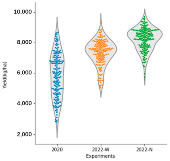
Figure 4.
Winter wheat yield distribution under different experiments. Python 3.9.12 was used to generate the violin plot. The violin plot could be used to express the wheat yield density distribution of different treatments. The violin plot on the periphery illustrated the overall distribution of winter wheat yield. It can be observed that wider areas of the plot correspond to higher data densities, indicating that there were more data points associated with those yield values. The accompanying scatter plot served to supplement the violin plot, with each point representing the yield value of an individual experimental plot. This combination of visualizations effectively conveys both the distribution and the variability in winter wheat yields across different experimental conditions.
The yield distribution of winter wheat harvested in 2020 was relatively wide, primarily ranging from 4000 kg/ha to 7500 kg/ha. The maximum yield density occurred at approximately 6900 kg/ha, with a small portion of yields exceeding 7500 kg/ha or falling below 4000 kg/ha. In contrast, the yield of winter wheat under different irrigation treatments in 2022 was predominantly concentrated in the range of 6500 kg/ha to 8500 kg/ha, with the highest density observed around 7500 kg/ha. Additionally, there were a few yields in the range of 5000 kg/ha to 6000 kg/ha, while very few exceeded 8000 kg/ha. For the year 2022, the yields of winter wheat under various nitrogen application treatments were mostly found between 7000 kg/ha and 9500 kg/ha, with the maximum yield density occurring around 8800 kg/ha. Though a small portion of yields fell between 6000 kg/ha and 7000 kg/ha, very few yields were recorded below 6000 kg/ha.
In summary, the majority of winter wheat plots with yields above 7000 kg/ha were concentrated in two experiments conducted in 2022, accounting for most of the experimental data. In contrast, those with yields below 5000 kg/ha were predominantly found in the experiments from 2020, with a relatively small quantity.
3.2. Correlation Between Multispectral Information and Winter Wheat Yield
From Figure 5, it is evident that only the near-infrared (NIR) reflectance displayed a positive correlation with winter wheat yield, while the other five types of multispectral information exhibited negative correlations. This is further illustrated in Table 6, which presents the correlation coefficients between various multispectral indices and winter wheat yield.
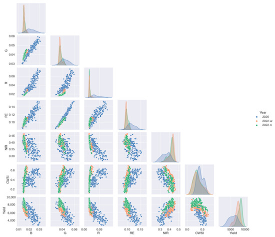
Figure 5.
Correlation analysis heat map in filling stage.

Table 6.
Correlation index between multispectral indices and winter wheat yield.
Analysis of the data under different irrigation amounts revealed that the correlation between red light reflectance and winter wheat yield reached its highest level at r = −0.80, occurring in 2020. Conversely, the correlation involving NIR reflectance was the weakest among the tested indices, with a coefficient of r = 0.6, observed in both 2020 and 2022. Additionally, the reflectance for blue light, green light, and red edge and the water stress index all shared a consistent correlation of r = −0.7, noted in both years.
When examining the effects of varying nitrogen fertilizer applications, the water stress index presented the weakest correlation with winter wheat yield, with a coefficient of r = −0.5. Reflectance measurements for blue light and the red edge yielded a similar correlation of r = −0.6. The correlation coefficients for green light and red reflectance were both r = −0.7, while NIR reflectance exhibited a positive correlation with winter wheat yield at r = 0.7.
Taking into account all wheat samples, it is notable that only the correlation between the crop water stress index (CWSI) and winter wheat yield did not reach the maximum value observed previously. In contrast, the correlation between NIR reflectance and winter wheat yield remained consistent, retaining its previous maximum value. Interestingly, the correlations between the reflectance of red light, green light, and red edge and winter wheat yield all increased to a value of 0.8, indicating a stronger positive association between these indices and winter wheat yield.
3.3. Findings on the Impact of Threshold (δ) in Pseudo Label Learning
The choice of the threshold (δ, measured in t/ha) significantly impacts the number and accuracy of trusted pseudo labels. Higher δ values, such as 0.2, allowed for a larger pool of trusted labels (188 in total). However, this came with increased deviations from the true values, with 58 labels exceeding a 10% error and 130 labels with an error of less than 10%. In contrast, lower δ values (e.g., 0.15 and 0.1) resulted in fewer trusted labels (111 and 50, respectively) and generally smaller errors, with only eight labels exceeding a 10% error at δ = 0.1.
The number of training rounds also affects the learning process. Fewer rounds led to less trust in the pseudo labels, resulting in smaller deviations from true values. However, increasing the number of rounds, especially at δ = 0.05, resulted in a cumulative increase in trusted labels—from 5 to 112 after 50 rounds. Despite this, the overall errors also increased with 19 labels showing errors greater than 10%, compared to a smaller error rate in fewer rounds.
Through extensive experimentation, a flexible δ strategy was established: for the first three rounds, δ was set to 0.05 minus 0.01 for each round, and afterwards, it was adjusted to 0.015, with a cap of 50 rounds for training. This methodology resulted in 84 trusted pseudo labels, 72 of which had an error of less than 10%, as illustrated in Figure 6. The distribution of these labels ranged from 3000 kg/ha to over 9000 kg/ha, predominantly exceeding 7000 kg/ha. Overall, the findings highlight the importance of selecting an appropriate δ value to optimize the accuracy of pseudo labels and the efficiency of the learning process, with higher δ values yielding more but less accurate labels and lower δ values providing fewer but more reliable ones.
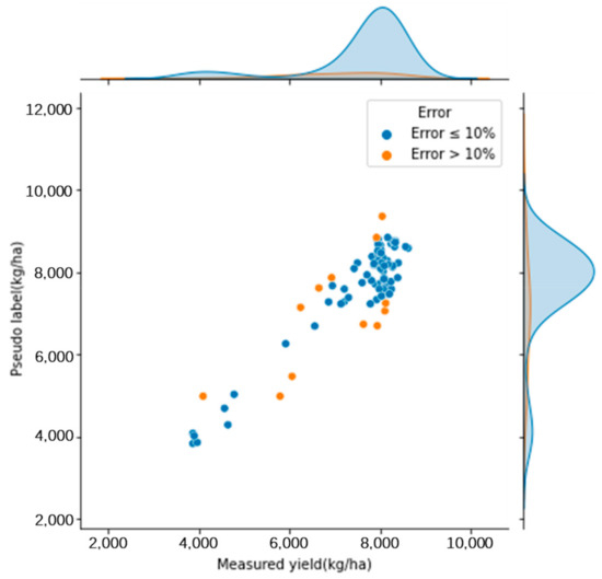
Figure 6.
Yield distribution of learned pseudo labels.
3.4. Performance Evaluation the Yield Prediction Using Multispectral Information
By training the random forest (RF) regressor with only 20% of the experimental data (108 data points) for the training set, 10% (54 data points) for the test set, and another 10% (54 data points) for the validation set, we obtained the following results. On the test dataset, we achieved an R2 of 0.81, RMSE of 681.02 kg/ha, and MAE of 568.97 kg/ha. For the validation dataset, which was never seen during training, we obtained an R2 of 0.79, RMSE of 736.24 kg/ha, and MAE of 585.85 kg/ha, as shown in Figure 7.
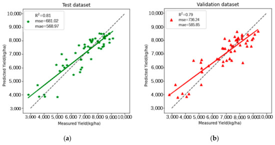
Figure 7.
The relationships between the ground-measured and predicted values of winter wheat yield obtained by RF. (a) Description of what is in the test dataset; (b) description of what is in the validation dataset.
The testing results indicated that the regressor’s performance on the validation dataset, based on the three statistical analysis metrics (R2, RMSE, and MAE), was not as strong as that on the test set.
After self-training, 84 pieces of data were added to the training set. Based on the expanded training set, a test with an = 0.84, RMSE = 627.94 kg/ha, and MAE = 516.94 kg/ha was conducted on the test dataset, a verification with an = 0.81, RMSE = 692.96 kg/ha, and MAE = 550.62 kg/ha was conducted on the validation dataset, as shown in Figure 8.
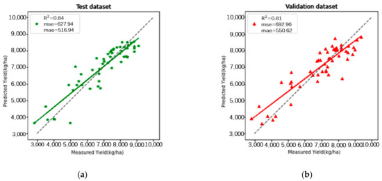
Figure 8.
The relationships between the ground-measured and predicted values of winter wheat yield obtained by a self-training random forest. (a) Description of what is in the test dataset; (b) description of what is in the validation dataset.
In terms of RMSE, compared to the random forest model, the self-training random forest model improved its performance by 7.8% in the test dataset and 5.6% in the validation dataset. In terms of MAE, compared to the random forest model, the self-training random forest model improved its performance by 9.1% in the test dataset and 6.0% in the validation dataset.
Whether it was on the test dataset or on the validation dataset, the self-training random forest algorithm performed better than the random forest algorithm without a self-training process. Taking into account the three indicators of the coefficient of determination for linear relationship (), RMSE, which is sensitive to outliers in the data, and MAE, which has better robustness against outliers, the self-training random forest model performed better in predicting winter wheat yield than the random forest model.
4. Discussion
4.1. Assessing the Relationship Between Multispectral Reflectance and Winter Wheat Yield
Under different external weather conditions (temperature, humidity, and precipitation), winter wheat varieties, and differences in watering and fertilization rates, the correlation between multispectral reflectance information of winter wheat and its yield was basically consistent. The more diverse the yield of the data, the clearer the correlation between the multispectral reflectance information of winter wheat and its yield. This indicated that using multispectral information from winter wheat to predict its yield was feasible. Various vegetation indices could be obtained from multispectral reflectance. Better estimation results could be achieved at the cost of higher computation complexity.
Although the winter wheat, used for analyzing correlations between its multispectral features and yield, had abundant variety, its sampling area was monotonous, all located in the same experimental field, which was slightly insufficient.
4.2. Challenges and Performance Factors in Self-Training Random Forest for Yield Prediction
From Figure 6, it was evident that self-training random forests could effectively annotate data to expand the training dataset. However, there was a need for optimization. As the number of self-training rounds increased, the labeled values tended to spread toward the edges, which could lead to greater errors. The accuracy of the labels annotated by the self-training random forest algorithm improved with the fitting quality of the initially trained regressor.
The highest proportion of yield in the source dataset fell between 7000 kg and 9000 kg per hectare in this experiment, and this segment of data was the most extensively learned by the self-training random forest algorithm. In the initial random forest training model, there was a significant discrepancy between the predicted yield and the actual yield for values ranging from 5000 kg to 7000 kg per hectare. The data learned by the self-training random forest algorithm also showed considerable deviation from the true values for this range.
These results indicated that the accuracy of the annotated data obtained through the self-training process depended not only on the distribution of the source data but also on the selection of the initial small-scale dataset and the training of the initial random forest model.
4.3. Enhancements in Winter Wheat Yield Prediction Through Self-Training Random Forest
A comparison of the results (refer to Figure 7 and Figure 8) from the random forest and self-training random forest revealed that the self-training random forest outperformed the traditional random forest in terms of data fitting (R2), prediction accuracy (RMSE), and outlier elimination (MAE). This suggests that the self-training random forest algorithm proposed in this article can enhance the accuracy of winter wheat yield predictions with only a small number of labeled datasets. The primary reason for this improvement was that the self-training process generated accurate pseudo labels for some unlabeled data, effectively expanding the training dataset and increasing the precision of winter wheat yield predictions.
After expanding the training set through self-training, the output estimation capabilities of the self-training random forest algorithm improved. A comparison of Figure 7 and Figure 8 indicated that while the random forest algorithm struggled with significant yield deviations, self-training led to noticeable improvements in predictions at those locations. However, the deviations remained substantial. This highlights that both the initial random forest training model and the original annotated dataset significantly influenced the final prediction accuracy of the self-training random forest algorithm.
5. Conclusions
Our test results indicated that the correlation between multispectral reflectance information and winter wheat yield was consistent across different weather conditions, irrigation treatments, nitrogen fertilization rates, and winter wheat varieties. This consistency suggests that using multispectral reflectance information to predict winter wheat yield is feasible. Moreover, the Pearson correlation between multispectral reflectance and yield was stronger across the three experimental datasets than within each individual dataset. This finding implies that, within the current land area, an increase in data enhances the relationship between the multispectral reflectance information of winter wheat and its yield.
Additionally, we discovered that the effectiveness of the initial random forest regression training and the selection of the initial training set could significantly impact the predictions of winter wheat yield and data annotation by the self-training random forest. Importantly, the application of the self-training random forest algorithm resulted in a notable improvement in performance, indicating the algorithm’s reliability in predicting winter wheat yield.
These findings highlight the importance of selecting the appropriate δ value to maximize both the accuracy of pseudo labels and the efficiency of the learning process. Higher δ values yield more labels but can also lead to increased error rates, while lower δ values produce fewer, more accurate labels, although at a slower learning pace. The adaptive δ strategy employed in this study effectively balanced these factors, resulting in a more reliable dataset for further training.
Although we tested over 30 winter wheat varieties under varying irrigation and nitrogen application rates, the current algorithm was only applied to small-scale plots, and data were collected exclusively from Henan Province. To establish a broader relationship between multispectral reflectance information—including the crop water stress index (CWSI)—and yield prediction across China and in more complex environments, future research will require the accumulation of more data under diverse conditions and in different regions.
Author Contributions
Conceptualization, Y.S. and B.M.; methodology, Y.S.; software, Y.S.; validation, H.Y., Z.L. and Q.L.; formal analysis, Q.L.; investigation, Z.C.; resources, W.W.; data curation, Z.C.; writing—original draft preparation, Y.S.; writing—review and editing, Y.S., Q.L. and B.M.; visualization, Z.L.; supervision, W.W.; project administration, W.W.; funding acquisition, Z.C. and H.Y. All authors have read and agreed to the published version of the manuscript.
Funding
This research was funded by the “National Science and Technology Major Project, grant number 2021ZD0110901”, “the Key Grant Technology Project of Henan, grant number 221100110700”, and “the Intelligent Irrigation Water and Fertilizer Digital Decision System and Regulation Equipment, grant number 2022YFD1900404”.
Data Availability Statement
The data presented in this study are available on request from the corresponding author due to regulations of the research institute.
Conflicts of Interest
The authors declare no conflicts of interest. The funders had no role in the design of this study; in the collection, analyses, or interpretation of data; in the writing of this manuscript; or in the decision to publish the results.
References
- Li, S.; Li, F.; Gao, M.; Li, Z.; Leng, P.; Duan, S.; Ren, J. A New Method for Winter Wheat Mapping Based on Spectral Reconstruction Technology. Remote Sens. 2021, 13, 1810. [Google Scholar] [CrossRef]
- Meraj, G.; Kanga, S.; Ambadkar, A.; Kumar, P.; Singh, S.K.; Farooq, M.; Johnson, B.A.; Rai, A.; Sahu, N. Assessing the Yield of Wheat Using Satellite Remote Sensing-Based Machine Learning Algorithms and Simulation Modeling. Remote Sens. 2022, 14, 3005. [Google Scholar] [CrossRef]
- Wu, Y.; Xu, W.; Huang, H.; Huang, J. Bayesian Posterior-Based Winter Wheat Yield Estimation at the Field Scale through Assimilation of Sentinel-2 Data into WOFOST Model. Remote Sens. 2022, 14, 3727. [Google Scholar] [CrossRef]
- Mezera, J.; Lukas, V.; Horniaček, I.; Smutný, V.; Elbl, J. Comparison of Proximal and Remote Sensing for the Diagnosis of Crop Status in Site-Specific Crop Management. Sensors 2022, 22, 19. [Google Scholar] [CrossRef] [PubMed]
- Marshall, M.; Belgiu, M.; Boschetti, M.; Pepe, M.; Stein, A.; Nelson, A. Field-level crop yield estimation with PRISMA and Sentinel-2. ISPRS J. Photogramm. Remote Sens. 2022, 187, 191–210. [Google Scholar] [CrossRef]
- Zhang, J.; Tian, H.; Wang, P.; Tansey, K.; Zhang, S.; Li, H. Improving wheat yield estimates using data augmentation models and remotely sensed biophysical indices within deep neural networks in the Guanzhong Plain, PR China. Comput. Electron. Agric. 2022, 192, 106616. [Google Scholar] [CrossRef]
- Prey, L.; Hanemann, A.; Ramgraber, L.; Seidl-Schulz, J.; Noack, P.O. UAV-Based Estimation of Grain Yield for Plant Breeding: Applied Strategies for Optimizing the Use of Sensors, Vegetation Indices, Growth Stages, and Machine Learning Algorithms. Remote Sens. 2022, 14, 6345. [Google Scholar] [CrossRef]
- Feng, H.; Tao, H.; Li, Z.; Yang, G.; Zhao, C. Comparison of UAV RGB imagery and hyperspectral remote-sensing data for monitoring winter-wheat growth. Remote Sens. 2022, 14, 3811. [Google Scholar] [CrossRef]
- Fei, S.; Hassan, M.A.; Xiao, Y.; Su, X.; Chen, Z.; Cheng, Q.; Duan, F.; Chen, R.; Ma, Y. UAV based multi sensor data fusion and machine learning algorithm for yield prediction in wheat. Precis. Agric. 2023, 24, 187–212. [Google Scholar] [CrossRef] [PubMed]
- Zeng, L.; Peng, G.; Meng, R.; Man, J.; Li, W.; Xu, B.; Lv, Z.; Sun, R. Wheat Yield Prediction Based on Unmanned Aerial Vehicles-Collected Red–Green–Blue Imagery. Remote Sens. 2021, 13, 2937. [Google Scholar] [CrossRef]
- Pang, A.; Chang, M.W.; Chen, Y. Evaluation of Random Forests (RF) for Regional and Local-Scale Wheat Yield Prediction in Southeast Australia. Sensors 2022, 22, 717. [Google Scholar] [CrossRef]
- Tanabe, R.; Matsui, T.; Tanaka, T.S. Winter wheat yield prediction using convolutional neural networks and UAV-based multispectral imagery. Field Crop. Res. 2023, 291, 108786. [Google Scholar] [CrossRef]
- Nayak, H.S.; Silva, J.V.; Parihar, C.M.; Krupnik, T.J.; Sena, D.R.; Kakraliya, S.K.; Jat, H.S.; Sidhu, H.S.; Sharma, P.C.; Jat, M.L.; et al. Interpretable machine learning methods to explain on-farm yield variability of high productivity wheat in Northwest India. Field Crop. Res. 2022, 287, 108640. [Google Scholar] [CrossRef]
- Zhou, Z.H. A brief introduction to weakly supervised learning. Natl. Sci. Rev. 2018, 5, 44–53. [Google Scholar] [CrossRef]
- Jones, H.G. Use of infrared thermometry for estimation of stomatal conductance as a possible aid to irrigation scheduling. Agric. For. Meteorol. 1999, 95, 139–149. [Google Scholar] [CrossRef]
- Mukherjee, S.; Awadallah, A.H. Uncertainty-aware Self-training for Text Classification with Few Labels. arXiv 2020, arXiv:2006.15315. [Google Scholar]
Disclaimer/Publisher’s Note: The statements, opinions and data contained in all publications are solely those of the individual author(s) and contributor(s) and not of MDPI and/or the editor(s). MDPI and/or the editor(s) disclaim responsibility for any injury to people or property resulting from any ideas, methods, instructions or products referred to in the content. |
© 2024 by the authors. Licensee MDPI, Basel, Switzerland. This article is an open access article distributed under the terms and conditions of the Creative Commons Attribution (CC BY) license (https://creativecommons.org/licenses/by/4.0/).