
Nearshore Bathymetry from ICESat-2 LiDAR and Sentinel-2 Imagery Datasets Using Physics-Informed CNN


Abstract
1. Introduction
2. Data Sources
2.1. ICESat-2 Data
2.2. Sentinel-2 Data
2.3. Validation Data
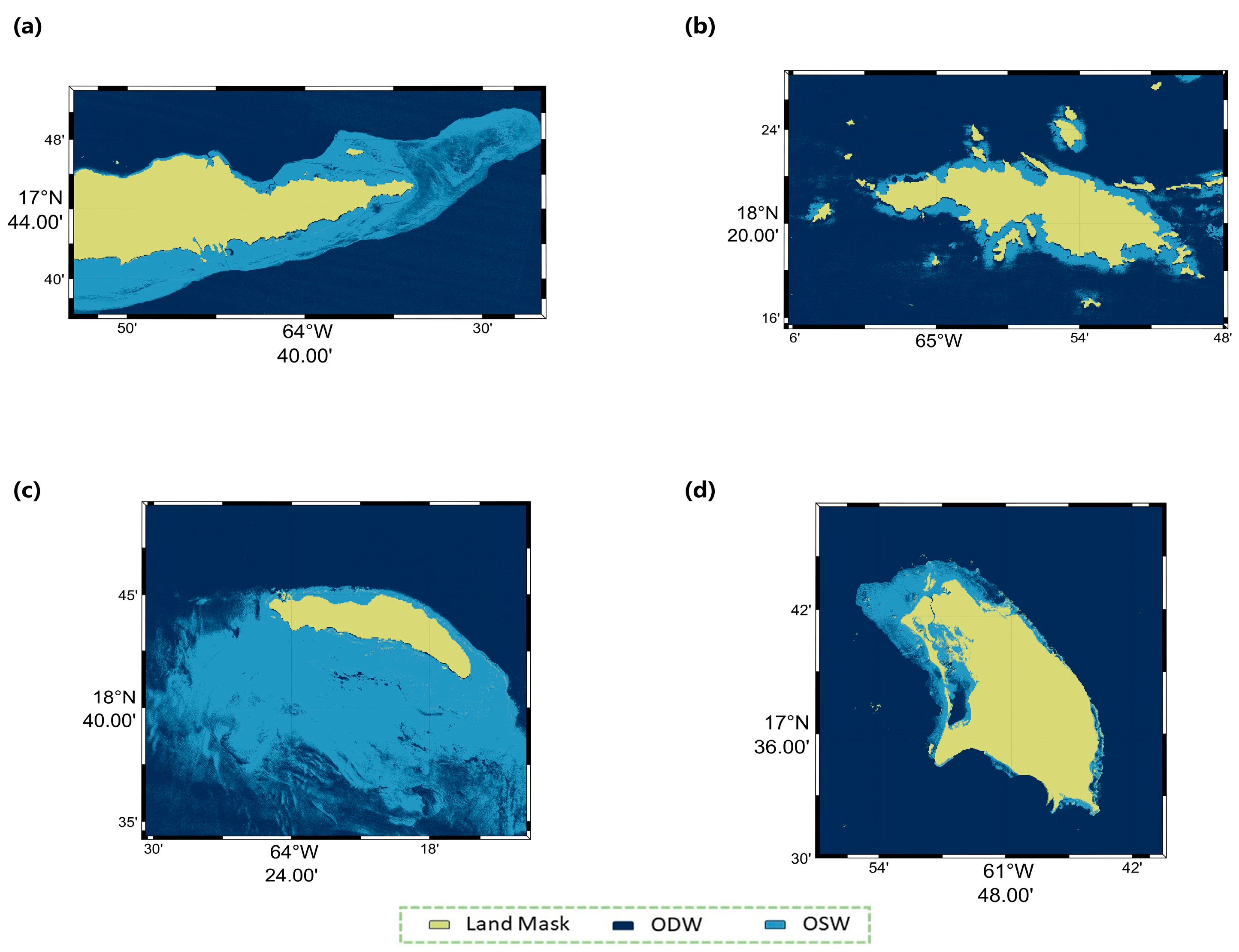
2.4. Study Regions
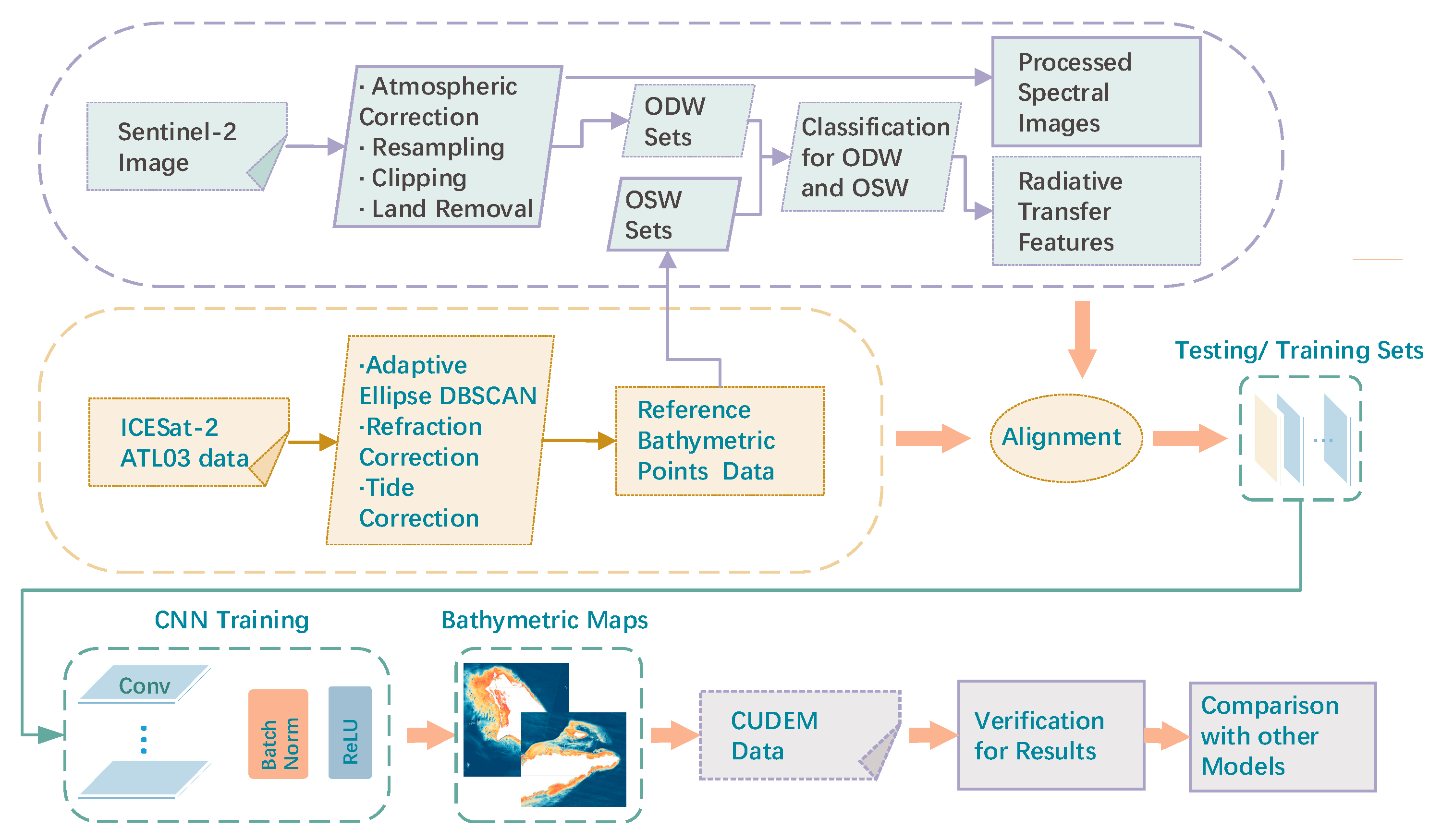
3. Method
3.1. PI-CNN Method Overview
3.2. Data Preparation
3.2.1. Bathymetric Data from ICESat-2
3.2.2. Multispectral Imagery Data from Sentinel-2
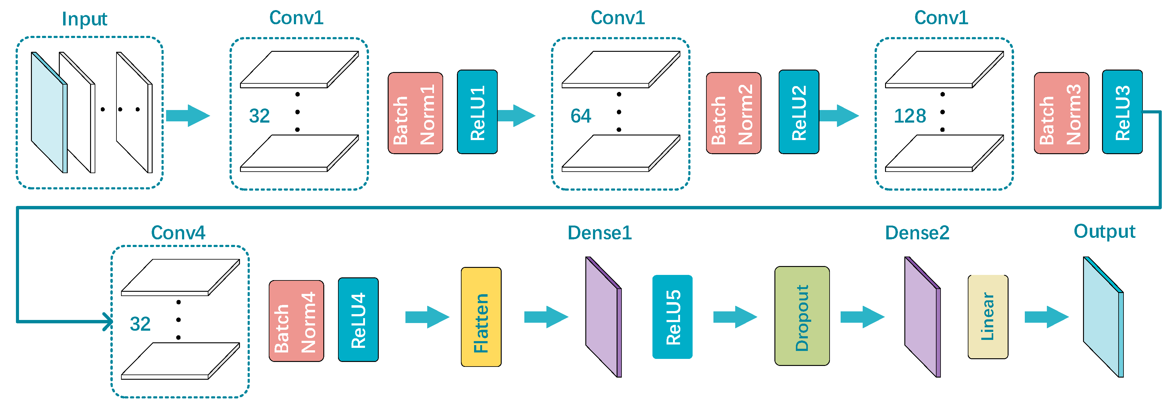
3.3. PI-CNN Model
3.3.1. Optical Physical Data Composition
3.3.2. PI-CNN Structure
3.4. Accuracy Assessment
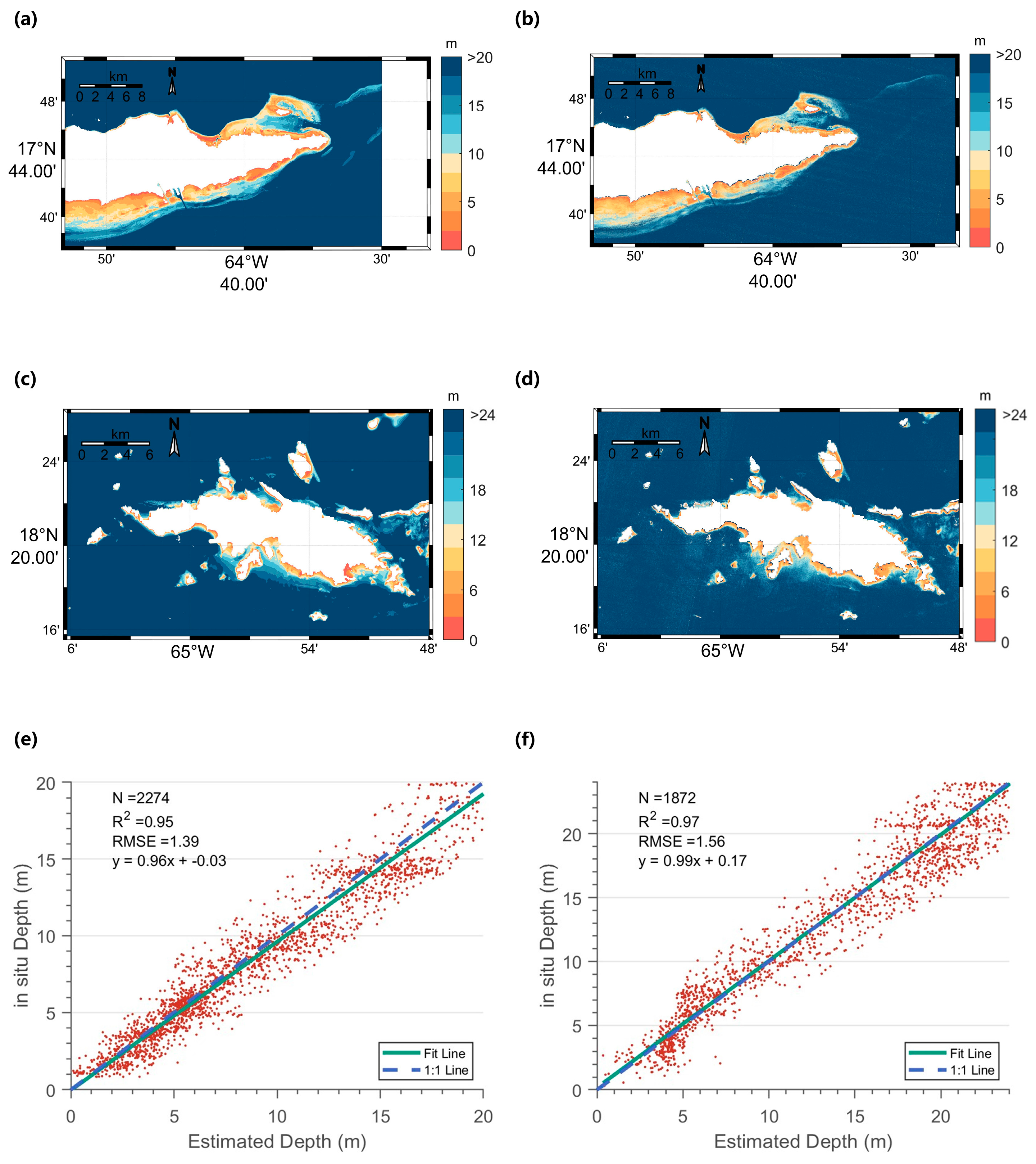
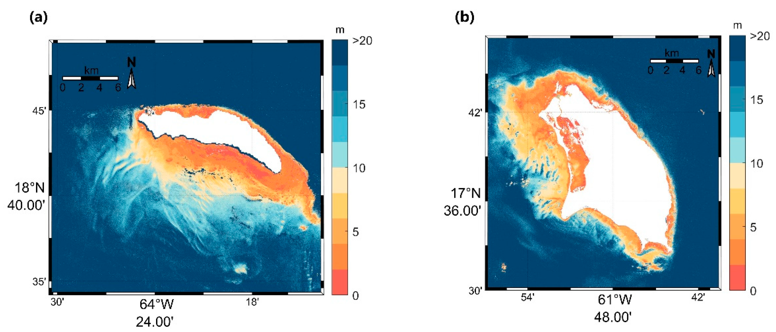
4. Model Results
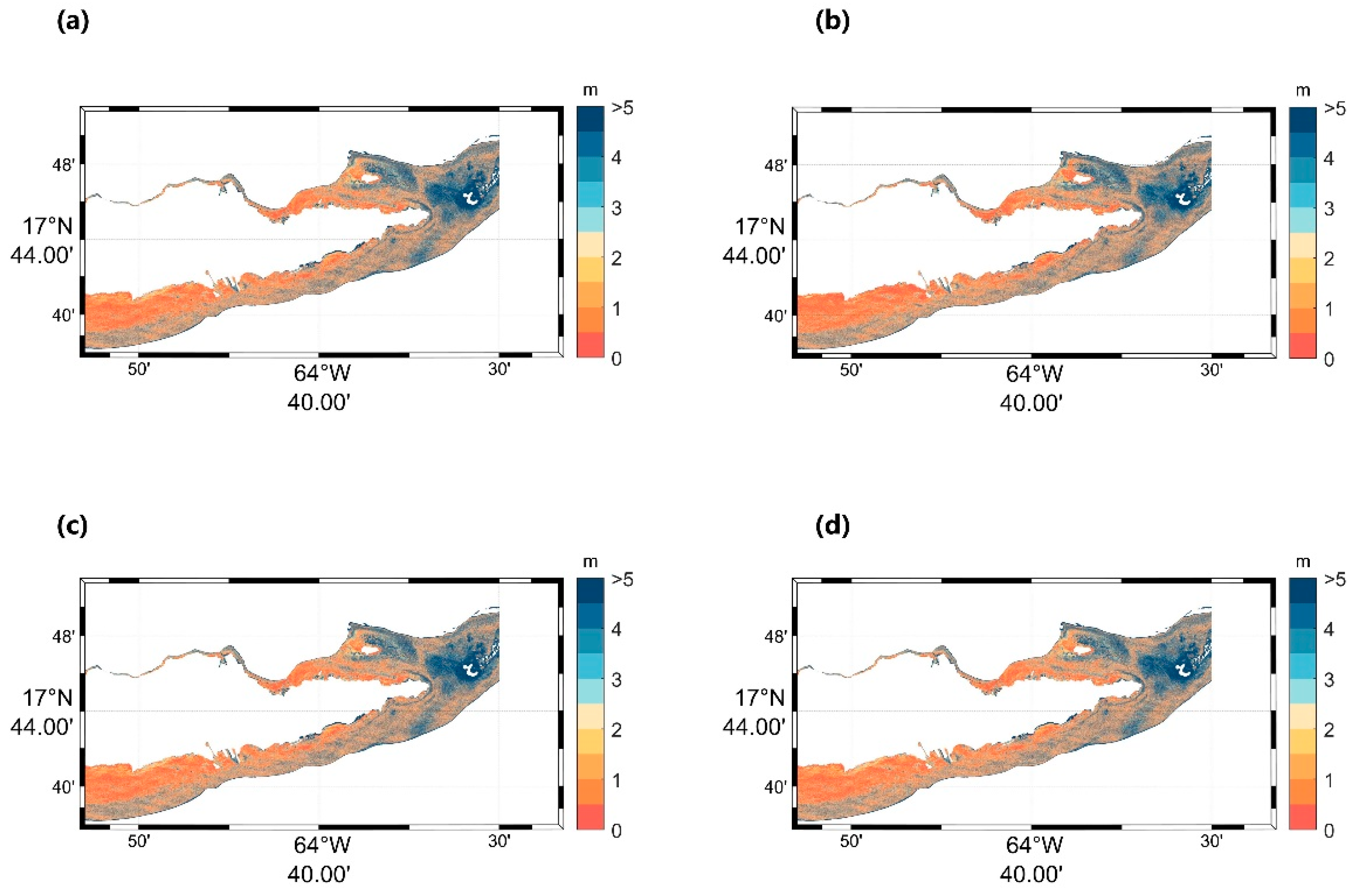
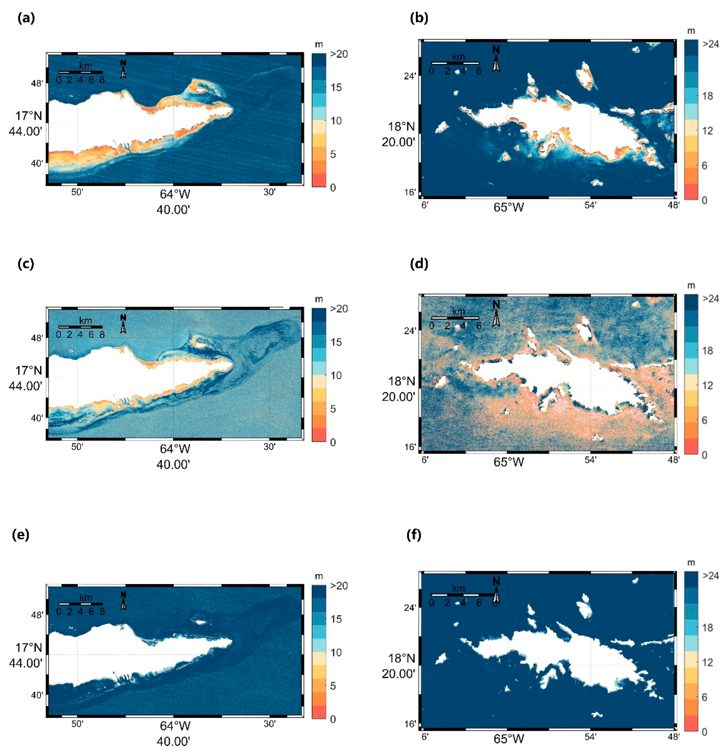
4.1. Lidar-Derived Bathymetric Results
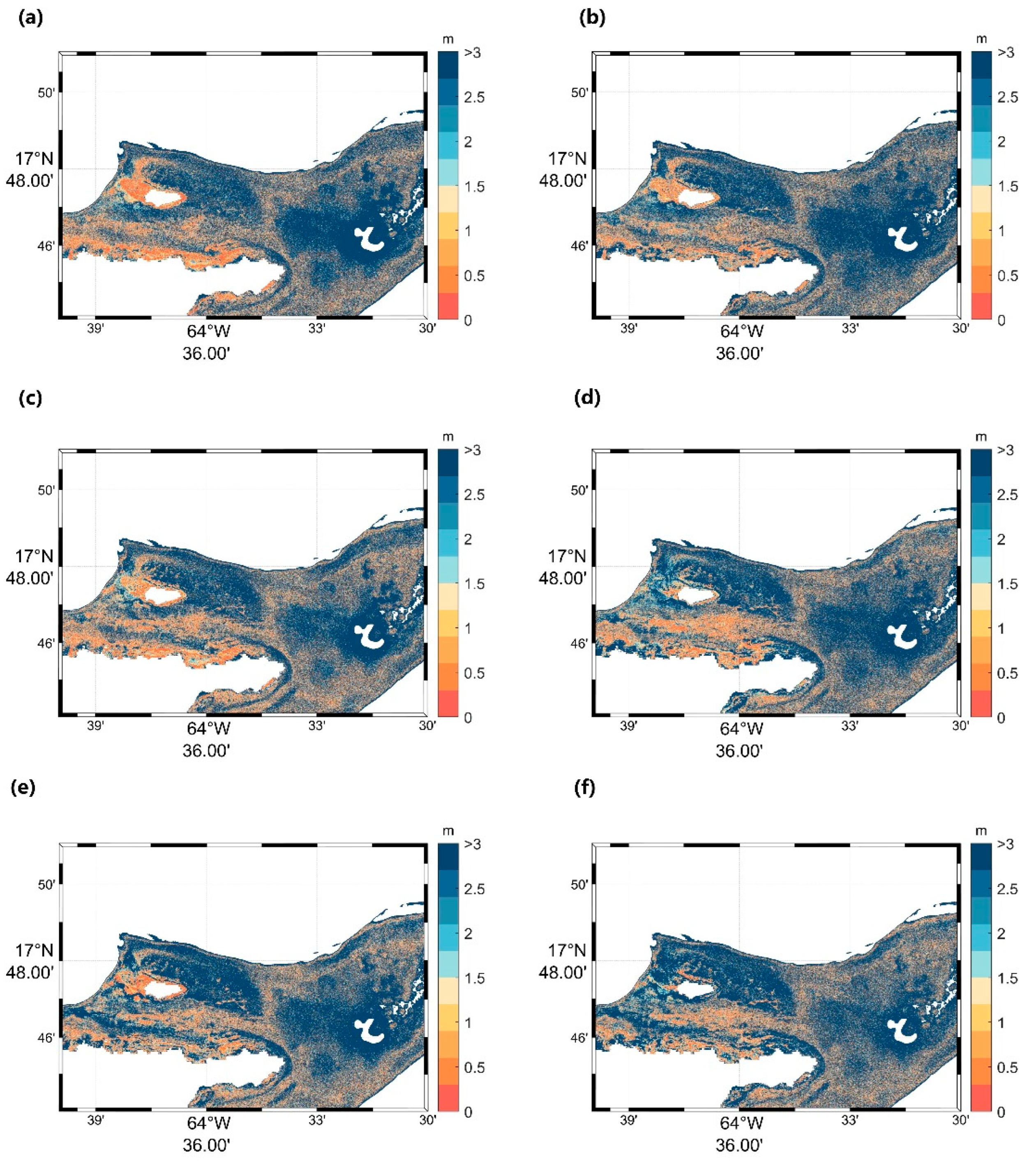
4.2. Optical Water Classification Results
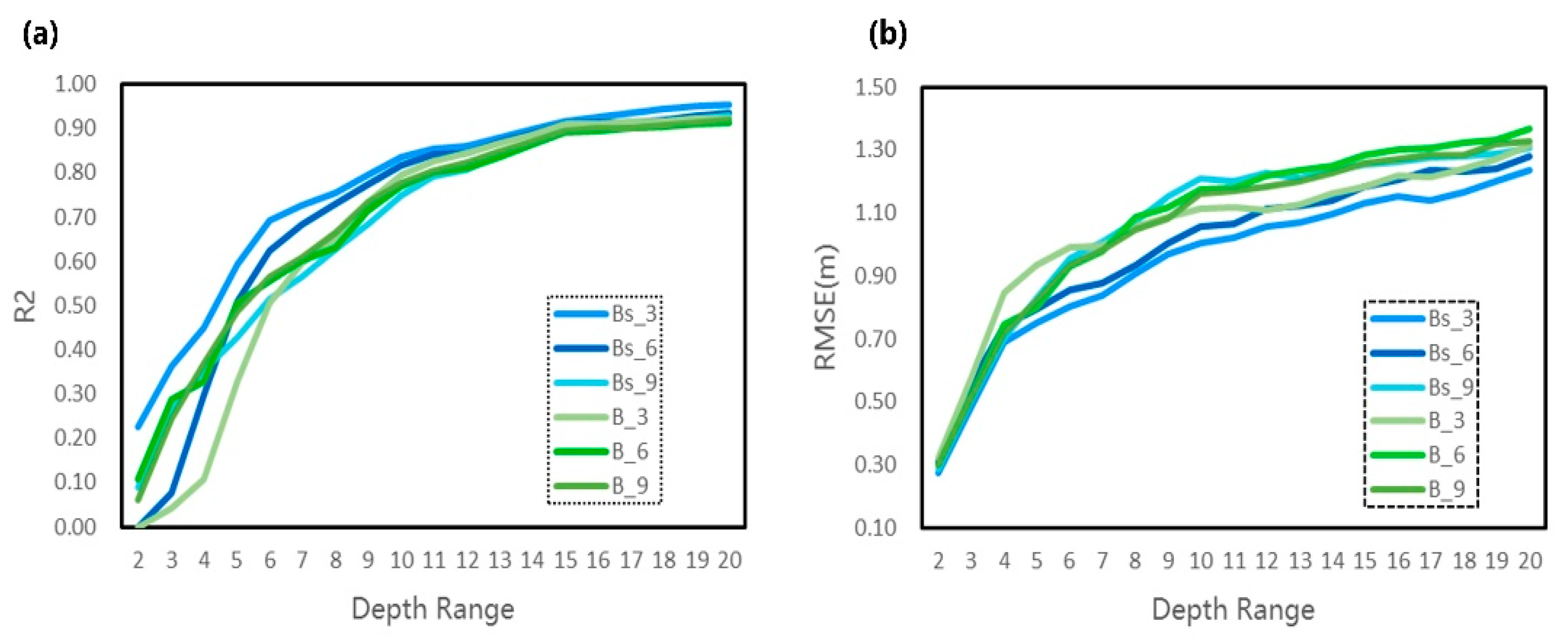
4.3. CNN Architectures Verification
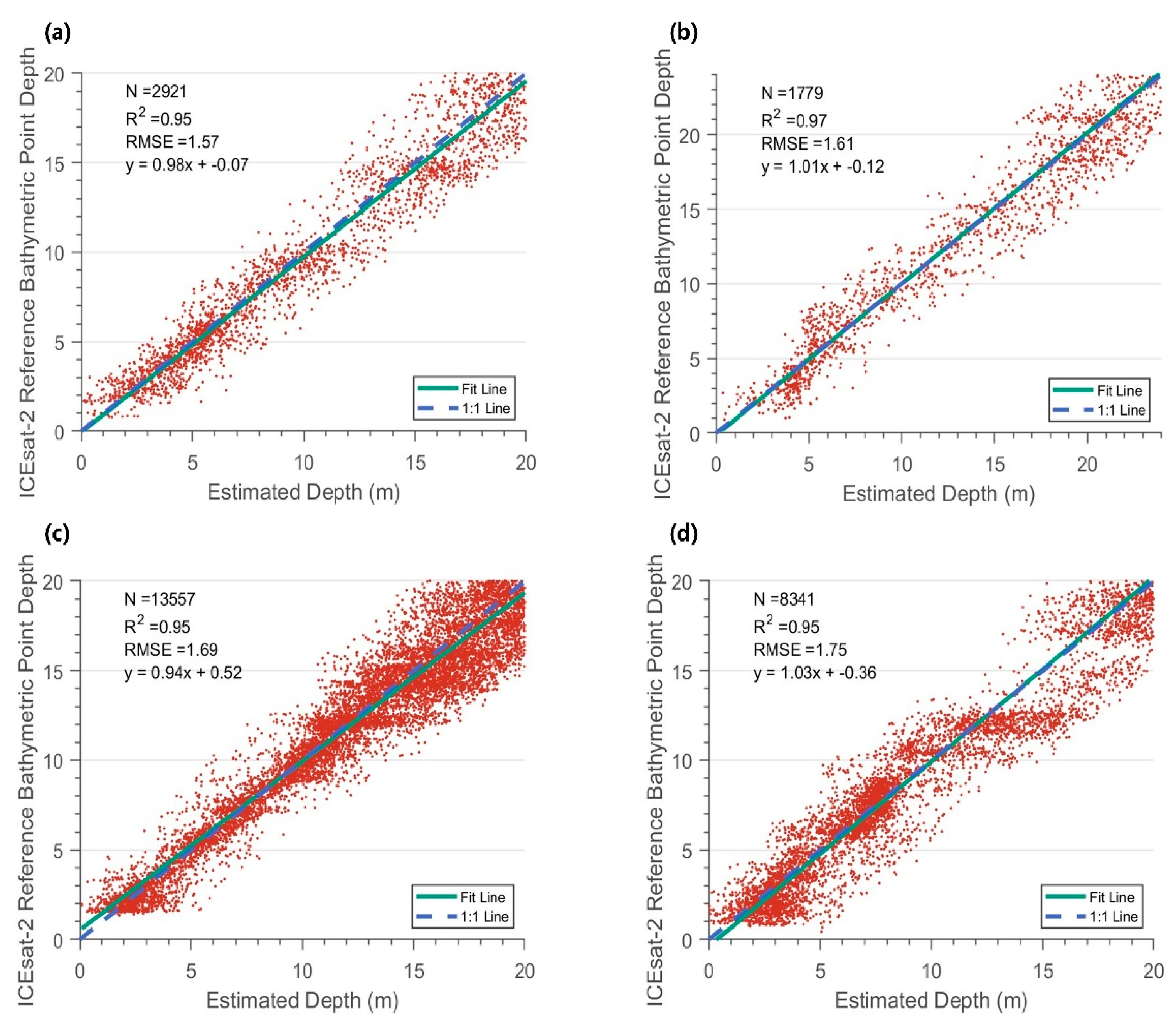
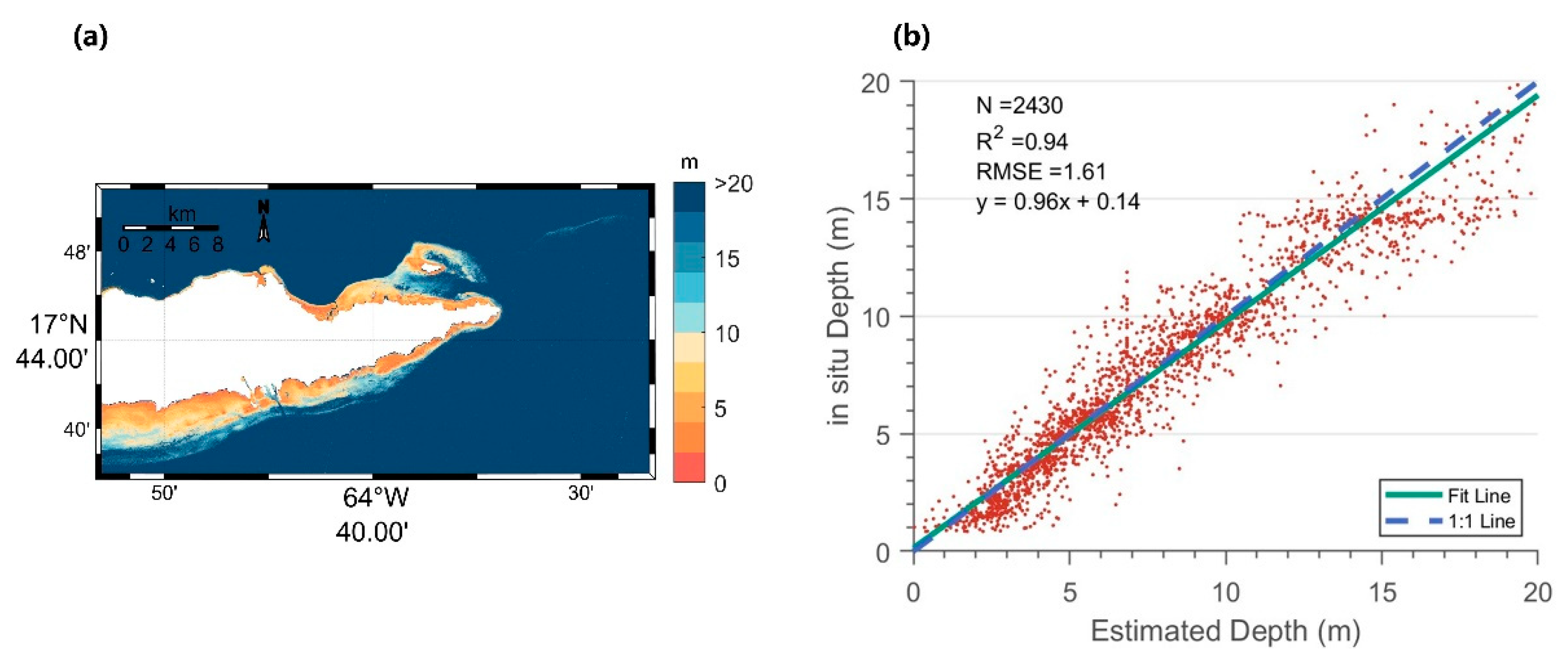
4.4. Bathymetric Estimates Validation
5. Discussion
5.1. Comparison with Different Band Combinations
5.2. Comparison with Other Bathymetric Retrieval Models
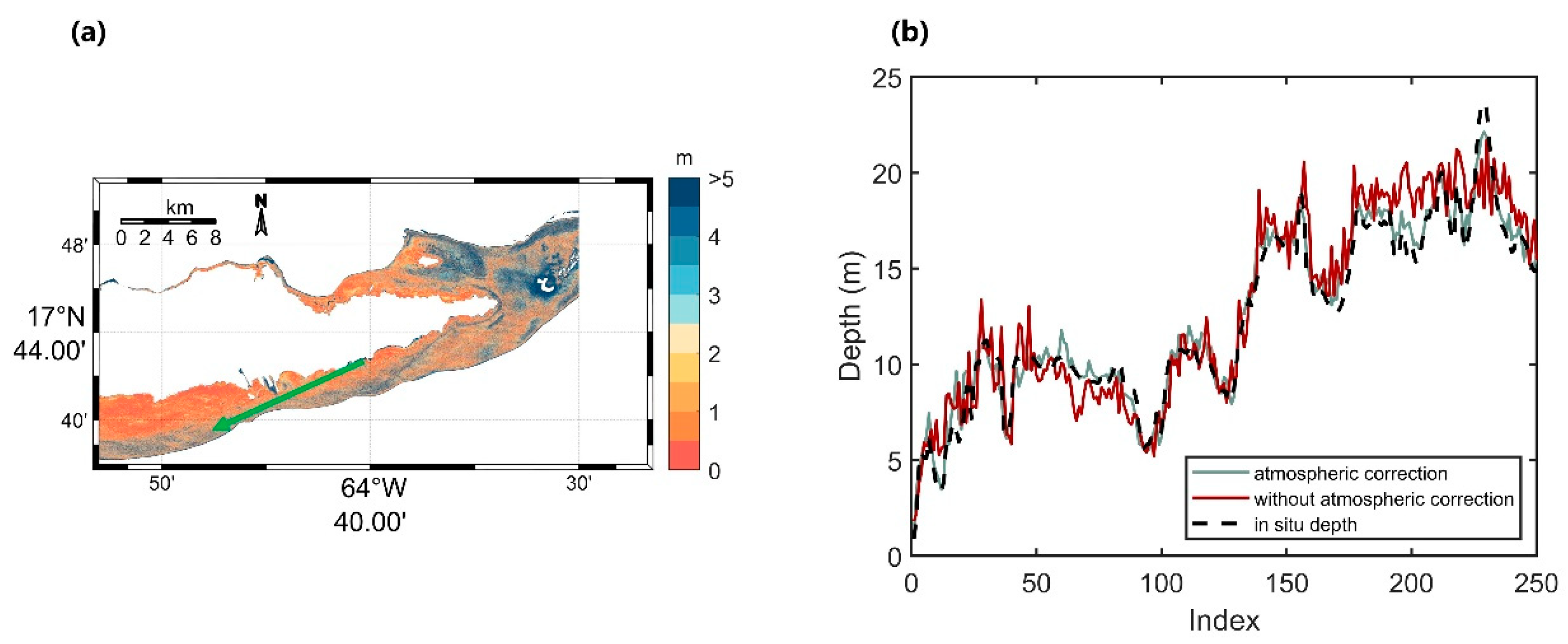
5.3. Atmospheric Correction
5.4. Analysis of Model Portability
6. Conclusions
- Our results demonstrate that the AE-DBSCAN method accurately tracks underwater topographic data. The accuracy and robustness of the generated bathymetric maps with the PI-CNN model are validated using CUDEM data from St. Croix and St. Thomas, with all experiments achieving an error less than 1.6 m.
- The PI-CNN model exhibits higher accuracy, and the RMSE using the PI-CNN model is reduced by 8.3% compared to the NN model in St. Thomas.
- With the NN method, avoiding atmospheric correction can result in more data products rather than the missing data due to atmospheric correction failure.
- When assessing SDB errors using uncorrected images, our proposed PI-CNN method achieves an accuracy of 1.61 m with an R2 value of 0.94, which is similar to the results obtained using corrected images, indicating minimal impact of atmospheric conditions on our approach’s performance.
Author Contributions
Funding
Data Availability Statement
Acknowledgments
Conflicts of Interest
References
- Benveniste, J.; Cazenave, A.; Vignudelli, S.; Fenoglio-Marc, L.; Shah, R.; Almar, R.; Andersen, O.; Birol, F.; Bonnefond, P.; Bouffard, J. Requirements for a coastal hazards observing system. Front. Mar. Sci. 2019, 6, 348. [Google Scholar] [CrossRef]
- Pacheco, A.; Horta, J.; Loureiro, C.; Ferreira, Ó. Retrieval of nearshore bathymetry from Landsat 8 images: A tool for coastal monitoring in shallow waters. Remote Sens. Environ. 2015, 159, 102–116. [Google Scholar] [CrossRef]
- Mayer, L.; Jakobsson, M.; Allen, G.; Dorschel, B.; Falconer, R.; Ferrini, V.; Lamarche, G.; Snaith, H.; Weatherall, P. The Nippon Foundation—GEBCO Seabed 2030 Project: The Quest to See the World’s Oceans Completely Mapped by 2030. Geosciences 2018, 8, 63. [Google Scholar] [CrossRef]
- Jawak, S.D.; Vadlamani, S.S.; Luis, A.J. A Synoptic Review on Deriving Bathymetry Information Using Remote Sensing Technologies: Models, Methods and Comparisons. Adv. Remote Sens. 2015, 4, 16. [Google Scholar] [CrossRef]
- Diesing, M.; Coggan, R.; Vanstaen, K. Widespread rocky reef occurrence in the central English Channel and the implications for predictive habitat mapping. Estuar. Coast. Shelf Sci. 2009, 83, 647–658. [Google Scholar] [CrossRef]
- Porskamp, P.; Rattray, A.; Young, M.; Ierodiaconou, D. Multiscale and hierarchical classification for benthic habitat mapping. Geosciences 2018, 8, 119. [Google Scholar] [CrossRef]
- Choi, C.; Kim, D.-J. Optimum baseline of a single-pass In-SAR system to generate the best DEM in tidal flats. IEEE J. Sel. Top. Appl. Earth Obs. Remote Sens. 2018, 11, 919–929. [Google Scholar] [CrossRef]
- Harris, P.T.; Baker, E.K. Why map benthic habitats? In Seafloor Geomorphology as Benthic Habitat; Elsevier: Amsterdam, The Netherlands, 2012; pp. 3–22. [Google Scholar]
- Almeida, L.P.; Almar, R.; Bergsma, E.W.; Berthier, E.; Baptista, P.; Garel, E.; Dada, O.A.; Alves, B. Deriving high spatial-resolution coastal topography from sub-meter satellite stereo imagery. Remote Sens. 2019, 11, 590. [Google Scholar] [CrossRef]
- Salameh, E.; Frappart, F.; Marieu, V.; Spodar, A.; Parisot, J.-P.; Hanquiez, V.; Turki, I.; Laignel, B. Monitoring sea level and topography of coastal lagoons using satellite radar altimetry: The example of the Arcachon Bay in the Bay of Biscay. Remote Sens. 2018, 10, 297. [Google Scholar] [CrossRef]
- Rahman, M.S.; Di, L. The state of the art of spaceborne remote sensing in flood management. Nat. Hazards 2017, 85, 1223–1248. [Google Scholar] [CrossRef]
- Casal, G.; Monteys, X.; Hedley, J.; Harris, P.; Cahalane, C.; McCarthy, T. Assessment of empirical algorithms for bathymetry extraction using Sentinel-2 data. Int. J. Remote Sens. 2018, 40, 2855–2879. [Google Scholar] [CrossRef]
- Han, W.; Zhang, X.; Wang, Y.; Wang, L.; Huang, X.; Li, J.; Wang, S.; Chen, W.; Li, X.; Feng, R.; et al. A survey of machine learning and deep learning in remote sensing of geological environment: Challenges, advances, and opportunities. ISPRS J. Photogramm. Remote Sens. 2023, 202, 87–113. [Google Scholar] [CrossRef]
- Caballero, I.; Stumpf, R.P. Retrieval of nearshore bathymetry from Sentinel-2A and 2B satellites in South Florida coastal waters. Estuar. Coast. Shelf Sci. 2019, 226, 106277. [Google Scholar] [CrossRef]
- Simpson, C.E.; Arp, C.D.; Sheng, Y.; Carroll, M.L.; Jones, B.M.; Smith, L.C. Landsat-derived bathymetry of lakes on the Arctic Coastal Plain of northern Alaska. Earth Syst. Sci. Data 2021, 13, 1135–1150. [Google Scholar] [CrossRef]
- Dörnhöfer, K.; Göritz, A.; Gege, P.; Pflug, B.; Oppelt, N. Water constituents and water depth retrieval from Sentinel-2A—A first evaluation in an oligotrophic lake. Remote Sens. 2016, 8, 941. [Google Scholar] [CrossRef]
- Chybicki, A. Mapping south baltic near-shore bathymetry using Sentinel-2 observations. Pol. Marit. Res. 2017, 24, 15–25. [Google Scholar] [CrossRef]
- Chybicki, A. Three-dimensional geographically weighted inverse regression (3GWR) model for satellite derived bathymetry using Sentinel-2 observations. Mar. Geod. 2018, 41, 1–23. [Google Scholar] [CrossRef]
- Almar, R.; Kestenare, E.; Reyns, J.; Jouanno, J.; Anthony, E.; Laibi, R.; Hemer, M.; Du Penhoat, Y.; Ranasinghe, R. Response of the Bight of Benin (Gulf of Guinea, West Africa) coastline to anthropogenic and natural forcing, Part1: Wave climate variability and impacts on the longshore sediment transport. Cont. Shelf Res. 2015, 110, 48–59. [Google Scholar] [CrossRef]
- Caballero, I.; Stumpf, R.P.; Meredith, A. Preliminary assessment of turbidity and chlorophyll impact on bathymetry derived from Sentinel-2A and Sentinel-3A satellites in South Florida. Remote Sens. 2019, 11, 645. [Google Scholar] [CrossRef]
- Dekker, A.G.; Phinn, S.R.; Anstee, J.; Bissett, P.; Brando, V.E.; Casey, B.; Fearns, P.; Hedley, J.; Klonowski, W.; Lee, Z.P. Intercomparison of shallow water bathymetry, hydro-optics, and benthos mapping techniques in Australian and Caribbean coastal environments. Limnol. Oceanogr. Methods 2011, 9, 396–425. [Google Scholar] [CrossRef]
- Hamylton, S.M.; Hedley, J.D.; Beaman, R.J. Derivation of high-resolution bathymetry from multispectral satellite imagery: A comparison of empirical and optimisation methods through geographical error analysis. Remote Sens. 2015, 7, 16257–16273. [Google Scholar] [CrossRef]
- Gao, J. Bathymetric mapping by means of remote sensing: Methods, accuracy and limitations. Prog. Phys. Geogr. Earth Environ. 2009, 33, 103–116. [Google Scholar] [CrossRef]
- Brando, V.E.; Anstee, J.M.; Wettle, M.; Dekker, A.G.; Phinn, S.R.; Roelfsema, C. A physics based retrieval and quality assessment of bathymetry from suboptimal hyperspectral data. Remote Sens. Environ. 2009, 113, 755–770. [Google Scholar] [CrossRef]
- Lee, Z.; Carder, K.L.; Mobley, C.D.; Steward, R.G.; Patch, J.S. Hyperspectral remote sensing for shallow waters: 2. Deriving bottom depths and water properties by optimization. Appl. Opt. 1999, 38, 3831–3843. [Google Scholar] [CrossRef] [PubMed]
- Casal, G.; Harris, P.; Monteys, X.; Hedley, J.; Cahalane, C.; McCarthy, T. Understanding satellite-derived bathymetry using Sentinel 2 imagery and spatial prediction models. GISci. Remote Sens. 2019, 57, 271–286. [Google Scholar] [CrossRef]
- Niroumand-Jadidi, M.; Bovolo, F.; Bruzzone, L.; Gege, P. Physics-based bathymetry and water quality retrieval using planetscope imagery: Impacts of 2020 COVID-19 lockdown and 2019 extreme flood in the Venice Lagoon. Remote Sens. 2020, 12, 2381. [Google Scholar] [CrossRef]
- Lyzenga, D.R. Passive remote sensing techniques for mapping water depth and bottom features. Appl. Opt. 1978, 17, 379–383. [Google Scholar] [CrossRef]
- Stumpf, R.P.; Holderied, K.; Sinclair, M. Determination of water depth with high-resolution satellite imagery over variable bottom types. Limnol. Oceanogr. 2003, 48, 547–556. [Google Scholar] [CrossRef]
- Niroumand-Jadidi, M.; Bovolo, F.; Bruzzone, L. SMART-SDB: Sample-specific multiple band ratio technique for satellite-derived bathymetry. Remote Sens. Environ. 2020, 251, 112091. [Google Scholar] [CrossRef]
- Traganos, D.; Poursanidis, D.; Aggarwal, B.; Chrysoulakis, N.; Reinartz, P. Estimating Satellite-Derived Bathymetry (SDB) with the Google Earth Engine and Sentinel-2. Remote Sens. 2018, 10, 859. [Google Scholar] [CrossRef]
- Caballero, I.; Stumpf, R. Towards Routine Mapping of Shallow Bathymetry in Environments with Variable Turbidity: Contribution of Sentinel-2A/B Satellites Mission. Remote Sens. 2020, 12, 451. [Google Scholar] [CrossRef]
- Forfinski-Sarkozi, N.A.; Parrish, C.E. Analysis of MABEL Bathymetry in Keweenaw Bay and Implications for ICESat-2 ATLAS. Remote Sens. 2016, 8, 772. [Google Scholar] [CrossRef]
- Forfinski-Sarkozi, N.A.; Parrish, C.E. Active-Passive Spaceborne Data Fusion for Mapping Nearshore Bathymetry. Photogramm. Eng. Remote Sens. 2019, 85, 281–295. [Google Scholar] [CrossRef]
- Li, Y.; Gao, H.; Jasinski, M.F.; Zhang, S.; Stoll, J.D. Deriving high-resolution reservoir bathymetry from ICESat-2 prototype photon-counting lidar and landsat imagery. IEEE Trans. Geosci. Remote Sens. 2019, 57, 7883–7893. [Google Scholar] [CrossRef]
- Neumann, T.A.; Martino, A.J.; Markus, T.; Bae, S.; Bock, M.R.; Brenner, A.C.; Brunt, K.M.; Cavanaugh, J.; Fernandes, S.T.; Hancock, D.W.; et al. The Ice, Cloud, and Land Elevation Satellite—2 mission: A global geolocated photon product derived from the Advanced Topographic Laser Altimeter System. Remote Sens. Environ. 2019, 233, 111325. [Google Scholar] [CrossRef] [PubMed]
- Neumann, T.; Scott, V.S.; Markus, T.; McGill, M. The Multiple Altimeter Beam Experimental Lidar (MABEL): An Airborne Simulator for the ICESat-2 Mission. J. Atmos. Ocean. Technol. 2013, 30, 345–352. [Google Scholar] [CrossRef]
- Zhang, W.; Xu, N.; Ma, Y.; Yang, B.; Zhang, Z.; Wang, X.H.; Li, S. A maximum bathymetric depth model to simulate satellite photon-counting lidar performance. ISPRS J. Photogramm. Remote Sens. 2021, 174, 182–197. [Google Scholar] [CrossRef]
- Ma, Y.; Xu, N.; Liu, Z.; Yang, B.; Yang, F.; Wang, X.H.; Li, S. Satellite-derived bathymetry using the ICESat-2 lidar and Sentinel-2 imagery datasets. Remote Sens. Environ. 2020, 250, 112047. [Google Scholar] [CrossRef]
- Chen, Y.; Le, Y.; Zhang, D.; Wang, Y.; Qiu, Z.; Wang, L. A photon-counting LiDAR bathymetric method based on adaptive variable ellipse filtering. Remote Sens. Environ. 2021, 256, 112326. [Google Scholar] [CrossRef]
- Xu, N.; Ma, X.; Ma, Y.; Zhao, P.; Yang, J.; Wang, X.H. Deriving Highly Accurate Shallow Water Bathymetry from Sentinel-2 and ICESat-2 Datasets by a Multitemporal Stacking Method. IEEE J. Sel. Top. Appl. Earth Obs. Remote Sens. 2021, 14, 6677–6685. [Google Scholar] [CrossRef]
- Xie, C.; Chen, P.; Pan, D.; Zhong, C.; Zhang, Z. Improved Filtering of ICESat-2 Lidar Data for Nearshore Bathymetry Estimation Using Sentinel-2 Imagery. Remote Sens. 2021, 13, 4303. [Google Scholar] [CrossRef]
- Auret, L.; Aldrich, C. Interpretation of nonlinear relationships between process variables by use of random forests. Miner. Eng. 2012, 35, 27–42. [Google Scholar] [CrossRef]
- Kaloop, M.R.; El-Diasty, M.; Hu, J.W.; Zarzoura, F. Hybrid Artificial Neural Networks for Modeling Shallow-Water Bathymetry via Satellite Imagery. IEEE Trans. Geosci. Remote Sens. 2022, 60, 5403811. [Google Scholar] [CrossRef]
- Liu, S.; Wang, L.; Liu, H.; Su, H.; Li, X.; Zheng, W. Deriving bathymetry from optical images with a localized neural network algorithm. IEEE Trans. Geosci. Remote Sens. 2018, 56, 5334–5342. [Google Scholar] [CrossRef]
- Misra, A.; Vojinovic, Z.; Ramakrishnan, B.; Luijendijk, A.; Ranasinghe, R. Shallow water bathymetry mapping using Support Vector Machine (SVM) technique and multispectral imagery. Int. J. Remote Sens. 2018, 39, 4431–4450. [Google Scholar] [CrossRef]
- Wang, Y.; Zhou, X.; Li, C.; Chen, Y.; Yang, L. Bathymetry Model Based on Spectral and Spatial Multifeatures of Remote Sensing Image. IEEE Geosci. Remote Sens. Lett. 2020, 17, 37–41. [Google Scholar] [CrossRef]
- Peng, K.; Xie, H.; Xu, Q.; Huang, P.; Liu, Z. A Physics-Assisted Convolutional Neural Network for Bathymetric Mapping Using ICESat-2 and Sentinel-2 Data. IEEE Trans. Geosci. Remote Sens. 2022, 60, 4210513. [Google Scholar] [CrossRef]
- Ai, B.; Wen, Z.; Wang, Z.; Wang, R.; Su, D.; Li, C.; Yang, F. Convolutional neural network to retrieve water depth in marine shallow water area from remote sensing images. IEEE J. Sel. Top. Appl. Earth Obs. Remote Sens. 2020, 13, 2888–2898. [Google Scholar] [CrossRef]
- Chen, H.; Yin, D.; Chen, J.; Chen, X.; Liu, S.; Liu, L. Stacked spectral feature space patch: An advanced spectral representation for precise crop classification based on convolutional neural network. Crop J. 2022, 10, 1460–1469. [Google Scholar] [CrossRef]
- Legleiter, C.J.; Overstreet, B.T. Mapping gravel bed river bathymetry from space. J. Geophys. Res. Earth Surf. 2012, 117, F04024. [Google Scholar] [CrossRef]
- Philpot, W.D. Bathymetric mapping with passive multispectral imagery. Appl. Opt. 1989, 28, 1569–1578. [Google Scholar] [CrossRef] [PubMed]
- Neumann, T.; Brenner, A.; Hancock, D.; Robbins, J.; Saba, J.; Harbeck, K.; Gibbons, A.; Lee, J.; Luthcke, S.; Rebold, T. Algorithm Theoretical Basis Document (ATBD) for Global Geolocated Photons ATL03; Goddard Space Flight Center: Greenbelt, MD, USA, 2018. [Google Scholar]
- Altamimi, Z.; Rebischung, P.; Métivier, L.; Collilieux, X. ITRF2014: A new release of the International Terrestrial Reference Frame modeling nonlinear station motions. J. Geophys. Res. Solid Earth 2016, 121, 6109–6131. [Google Scholar] [CrossRef]
- Markus, T.; Neumann, T.; Martino, A.; Abdalati, W.; Brunt, K.; Csatho, B.; Farrell, S.; Fricker, H.; Gardner, A.; Harding, D.; et al. The Ice, Cloud, and land Elevation Satellite-2 (ICESat-2): Science requirements, concept, and implementation. Remote Sens. Environ. 2017, 190, 260–273. [Google Scholar] [CrossRef]
- Drusch, M.; Del Bello, U.; Carlier, S.; Colin, O.; Fernandez, V.; Gascon, F.; Hoersch, B.; Isola, C.; Laberinti, P.; Martimort, P.; et al. Sentinel-2: ESA’s Optical High-Resolution Mission for GMES Operational Services. Remote Sens. Environ. 2012, 120, 25–36. [Google Scholar] [CrossRef]
- Richter, R.; Wang, X.; Bachmann, M.; Schläpfer, D. Correction of cirrus effects in Sentinel-2 type of imagery. Int. J. Remote Sens. 2011, 32, 2931–2941. [Google Scholar] [CrossRef]
- Amante, C.J.; Love, M.; Carignan, K.; Sutherland, M.G.; MacFerrin, M.; Lim, E. Continuously Updated Digital Elevation Models (CUDEMs) to Support Coastal Inundation Modeling. Remote Sens. 2023, 15, 1702. [Google Scholar] [CrossRef]
- Ester, M.; Kriegel, H.-P.; Sander, J.; Xu, X. A density-based algorithm for discovering clusters in large spatial databases with noise. In Proceedings of the Second International Conference on Knowledge Discovery and Data Mining, Portland, OR, USA, 2–4 August 1996; pp. 226–231. [Google Scholar]
- Parrish, C.E.; Magruder, L.A.; Neuenschwander, A.L.; Forfinski-Sarkozi, N.; Alonzo, M.; Jasinski, M. Validation of ICESat-2 ATLAS Bathymetry and Analysis of ATLAS’s Bathymetric Mapping Performance. Remote Sens. 2019, 11, 1634. [Google Scholar] [CrossRef]
- Legleiter, C.J.; Roberts, D.A.; Lawrence, R.L. Spectrally based remote sensing of river bathymetry. Earth Surf. Process. Landf. 2009, 34, 1039–1059. [Google Scholar] [CrossRef]
- Lai, W.; Lee, Z.; Wang, J.; Wang, Y.; Garcia, R.; Zhang, H. A Portable Algorithm to Retrieve Bottom Depth of Optically Shallow Waters from Top-of-Atmosphere Measurements. J. Remote Sens. 2022, 2022, 9831947. [Google Scholar] [CrossRef]
- Kirk, J.T. Light and Photosynthesis in Aquatic Ecosystems; Cambridge University Press: Cambridge, UK, 1994. [Google Scholar]
- Mueller, L.; O’Reilly, J.; Hooker, S.; Firestone, E. SeaWiFS postlaunch calibration and validation analyses. SeaWiFS Algorithm Diffus. Attenuation Coeff. K (490) Using Water-Leaving Radiances; NASA Goddard Space Flight Center: Washington, DC, USA, 2000; Volume 490, pp. 24–27. [Google Scholar]
- Lee, Z.-P.; Darecki, M.; Carder, K.L.; Davis, C.O.; Stramski, D.; Rhea, W.J. Diffuse attenuation coefficient of downwelling irradiance: An evaluation of remote sensing methods. J. Geophys. Res. Ocean. 2005, 110, C02017. [Google Scholar] [CrossRef]
- Xie, C.; Chen, P.; Zhang, Z.; Pan, D. Satellite-derived bathymetry combined with Sentinel-2 and ICESat-2 datasets using machine learning. Front. Earth Sci. 2023, 11, 1111817. [Google Scholar] [CrossRef]
- Lyzenga, D.R. Shallow-water bathymetry using combined lidar and passive multispectral scanner data. Int. J. Remote Sens. 1985, 6, 115–125. [Google Scholar] [CrossRef]
- Robinson, I.S. Discovering the Ocean from Space: The Unique Applications of Satellite Oceanography; Springer Science & Business Media: Berlin/Heidelberg, Germany, 2010. [Google Scholar]
- Toming, K.; Kutser, T.; Laas, A.; Sepp, M.; Paavel, B.; Nõges, T. First Experiences in Mapping Lake Water Quality Parameters with Sentinel-2 MSI Imagery. Remote Sens. 2016, 8, 640. [Google Scholar] [CrossRef]
- Platt, U.; Pfeilsticker, K.; Vollmer, M. Radiation and Optics in the Atmosphere. In Springer Handbook of Lasers and Optics; Springer: Berlin/Heidelberg, Germany, 2007; p. 1165. [Google Scholar]
- Müller, W. Sen2Cor Software Release Note; European Space Agency: Paris, France, 2018. [Google Scholar]
- Eugenio, F.; Marcello, J.; Martin, J. High-Resolution Maps of Bathymetry and Benthic Habitats in Shallow-Water Environments Using Multispectral Remote Sensing Imagery. IEEE Trans. Geosci. Remote Sens. 2015, 53, 3539–3549. [Google Scholar] [CrossRef]


| St. Croix | St. Thomas | Anegada | Barbuda | |
|---|---|---|---|---|
| Longitude Limits | 64.89~64.44°W | 65.11~64.80°W | 64.51~64.23°W | 61.95~61.67°W |
| Latitude Limits | 17.63~17.85°N | 18.26~18.44°N | 18.57~18.82°N | 17.50~17.79°N |
| Area (km2) | ~36.71 × 31.54 | ~32.03 × 20.64 | ~55.21 × 54.86 | ~40.67 × 40.41 |
| ICESat-2 data Time | 21 December 2018—04:39:25 19 January 2019—03:15:23 19 April 2019—22:55:19 17 June 2019—08:01:34 16 September 2019—03:41:25 15 September 2021—04:57:28 | 22 November 2018—06:03:25 15 December 2019—23:21:13 13 December 2020—06:00:25 18 May 2021—10:41:29 | 20 October 2018—07:35:37 15 May 2019—09:33:56 14 August 2019—05:13:38 12 September 2019—03:49:44 15 December 2019—23:21:13 18 June 2020—02:38:09 14 August 2020—23:50:15 | 3 May 2019—09:58:56 2 August 2019—05:38:37 31 August 2019—04:14:43 1 November 2019—01:18:32 29 November 2019—23:54:33 |
| Sentinel-2 data Time | 13 August 2019 | 21 November 2018 | 19 April 2020 | 23 October 2021 |
| Band Name | Central Wavelength (nm) | Band Detail | Bands Name | Band Detail |
|---|---|---|---|---|
| Bs_3 | B2 Blue 490, B3 Green 560, B4 Red 665 | B2, B3, B4, , , , | B_3 | B2, B3, B4, |
| Bs_6 | B2 Blue 490, B3 Green 560, B4 Red 665, B8 NIR 842, B11 SWIR1 1610, B12 SWIR2 2190 | B2, B3, B4, B8, B11, B12, , , , | B_6 | B2, B3, B4, B8, B11, B12, |
| Bs_9 | B2 Blue 490, B3 Green 560, B4 Red 665, B5 VRE1 705, B6 VRE2 740, B7 VRE3 783, B8 NIR 842, B11 SWIR1 1610, B12 SWIR2 2190 | B2, B3, B4, B5, B6, B7, B8, B11, B12, , , , | B_9 | B2, B3, B4, B5, B6, B7, B8, B11, B12, |
| Regions | St. Croix | St. Thomas | Anegada | Barbuda |
|---|---|---|---|---|
| Accuracy (%) | 95.6 | 95.1 | 96.3 | 94.8 |
Disclaimer/Publisher’s Note: The statements, opinions and data contained in all publications are solely those of the individual author(s) and contributor(s) and not of MDPI and/or the editor(s). MDPI and/or the editor(s) disclaim responsibility for any injury to people or property resulting from any ideas, methods, instructions or products referred to in the content. |
© 2024 by the authors. Licensee MDPI, Basel, Switzerland. This article is an open access article distributed under the terms and conditions of the Creative Commons Attribution (CC BY) license (https://creativecommons.org/licenses/by/4.0/).
Share and Cite
Xie, C.; Chen, P.; Zhang, S.; Huang, H. Nearshore Bathymetry from ICESat-2 LiDAR and Sentinel-2 Imagery Datasets Using Physics-Informed CNN. Remote Sens. 2024, 16, 511. https://doi.org/10.3390/rs16030511
Xie C, Chen P, Zhang S, Huang H. Nearshore Bathymetry from ICESat-2 LiDAR and Sentinel-2 Imagery Datasets Using Physics-Informed CNN. Remote Sensing. 2024; 16(3):511. https://doi.org/10.3390/rs16030511
Chicago/Turabian StyleXie, Congshuang, Peng Chen, Siqi Zhang, and Haiqing Huang. 2024. "Nearshore Bathymetry from ICESat-2 LiDAR and Sentinel-2 Imagery Datasets Using Physics-Informed CNN" Remote Sensing 16, no. 3: 511. https://doi.org/10.3390/rs16030511
APA StyleXie, C., Chen, P., Zhang, S., & Huang, H. (2024). Nearshore Bathymetry from ICESat-2 LiDAR and Sentinel-2 Imagery Datasets Using Physics-Informed CNN. Remote Sensing, 16(3), 511. https://doi.org/10.3390/rs16030511