Abstract
The frequency–azimuth (FRAZ) spectrum is a critical characteristic in passive target detection and tracking, as it encapsulates information regarding the signal’s frequency and azimuth. However, due to the inherent limitations in the sonar array’s physical aperture and the analysis time of the system, the signal often suffers from undersampling in both spatial and temporal dimensions. This undersampling leads to energy leakage across the azimuth and frequency domains, adversely affecting the resolution of the FRAZ spectrum. Such a reduction in resolution hampers multitarget resolution and feature extraction. To address these challenges, this study introduces a deconvolution-based FRAZ spectrum estimation method tailored for uniform linear arrays. The proposed method initiates by decoupling the azimuth and frequency in the FRAZ spectrum, forming a two-dimensional point scattering function that possesses shift-invariance. Subsequent to this, the power spectrum and the two-dimensional point scattering function undergo deconvolution using the Richardson–Lucy (R–L) iterative algorithm. The final stage involves calculating the signal azimuths and frequencies based on the deconvolution results from the preceding step. Comparative analyses involving simulations and sea test results reveal that the proposed method achieves a narrower main lobe width and diminished background noise in contrast to traditional FRAZ spectrum estimation techniques. This improvement is instrumental in minimizing the target’s energy leakage in both the azimuth and frequency domains.
1. Introduction
In the realm of array signal processing, the uniform linear array is a prevalent configuration, extensively utilized across various applications in radar, sonar, and related fields. The estimation of received signal parameters using uniform linear arrays represents a primary area of inquiry in array signal processing [1,2]. These parameters predominantly encompass aspects such as the frequency, azimuth, and Doppler frequency. In the context of passive processing modes, the absence of prior information about the signal often necessitates the joint estimation of multiple signal parameters. Among these, the concurrent estimation of signal azimuth and frequency has emerged as a focal point of research within the array signal processing domain [3].
The joint estimation of azimuth and frequency in received signals is a complex multiparameter problem. Over the past three decades, research in the joint estimation of azimuth and frequency parameters has advanced significantly. Key algorithms in this domain include 2D-MVDR [4,5], 2D-MUSIC [6,7,8,9], and 2D-ESPRIT [10,11,12]. The 2D-MVDR and 2D-MUSIC algorithms derive results through constructing a power spectrum function and conducting scans across the azimuth and frequency. While these methods are known for their precision, they require substantial computational effort. The 2D-ESPRIT algorithm, leveraging subspace rotation invariant technology, circumvents the extensive computational demands associated with scanning. However, it necessitates an additional parameter pairing operation and is characterized by its high complexity.
Aiming at the problems existing in the joint estimation algorithm of frequency and azimuth parameters, many scholars have carried out in-depth research. The authors of [13] constructed a two-dimensional autoregressive model based on observational data and estimated the signal frequency and azimuth according to a two-dimensional linear prediction. Reference [14] presented the joint estimation of the frequency and azimuth via establishing the matrix of direction of the azimuth, which requires less computation. This approach has received some attention. The above algorithms are all based on Nyquist sampling. In order to reduce the cost pressure of A/D conversion, a joint estimation algorithm of frequency and method based on sparse sampling conditions has been proposed [15,16,17,18]. In [19], a low-rank recovery method was proposed under the framework of two-dimensional spatial–temporal sparse sampling. The accuracy of parameter estimation was improved, but the complexity of the sampling structure was increased. By extending the dimensions of the covariance matrix in space and time, the authors of [20] improved the degree of freedom in the system, which can then estimate a greater number of sources, but the accuracy of the parameter estimation is reduced.
In practical engineering applications, where robustness and real-time performance are critical, the frequency domain beamforming method using preformed multi-beams is typically employed. This approach is utilized to ascertain the frequency–azimuth power spectrum, thereby retrieving the signal’s frequency and azimuth information. FRAZ is crucial for passive target detection [21,22]. Nevertheless, challenges arise due to the limited aperture of the array, leading to insufficient spatial sampling. This limitation results in energy leakage in beams other than the target beam [23]. Concurrently, the array system also faces restrictions in the time domain due to inadequate analysis time, causing issues in the frequency dimension of the line spectrum, such as energy leakage and resolution reduction [24,25,26].
To mitigate the signal energy leakage in the azimuth, conventional beamforming is combined with the R–L deconvolution algorithm to estimate the target’s azimuth of direction [27,28,29,30]. In this method, the beam pattern is treated as a point scattering function (PSF) in deconvolution, and the target azimuth is determined using the R–L iterative algorithm. This estimation technique, when compared to conventional beam forming (CBF), achieves a narrower main lobe and reduced side lobes. These features are instrumental in suppressing azimuth energy leaks for the target. However, its applicability is limited to arrays whose beam patterns exhibit shift-invariant properties. The deconvolution algorithm is further extended from the azimuth domain to the frequency domain. This extension effectively eliminates the spectrum leakage caused by the window function. It is achieved by deconvolving the power spectrum of the finite-length signal with the power spectrum of the window function, resulting in enhanced frequency resolution [31,32].
The application of a deconvolution algorithm across both azimuth and frequency domains effectively suppresses energy leakage while enhancing the resolution in the azimuth and frequency. This paper proposes a deconvolution-based FRAZ spectrum estimation algorithm for uniform linear arrays, specifically designed to address energy leakage issues in both the azimuth and frequency domains of the FRAZ spectrum. It is adept at concurrently mitigating energy leakage in the line spectrum across the azimuth and frequency domains.
This paper begins by introducing the two-dimensional Richardson–Lucy (2-D R–L) deconvolution algorithm as a foundational element. Subsequently, it elaborates on the FRAZ spectrum estimation method, which is grounded in deconvolution principles. The final part of this paper demonstrates the efficacy of this novel method through presenting numerical simulations and experimental data analysis.
2. Methods
2.1. Two-Dimensional R–L Deconvolution Algorithm
In the context of two-dimensional systems, in which represent the reference variables, the behavior of a two-dimensional signal passing through a linear shift-invariant system is of interest. The system function of this system is denoted as . Consequently, the system’s output, , can be mathematically represented as the two-dimensional convolution of the input signal and the system function . This convolution process is a fundamental operation when analyzing the interaction between the signal and the system.
where the symbol “” represents two-dimensional convolution. In this context, characterizes the system and is assumed to be known, while is measurable, and the signal is to be estimated. According to deconvolution theory, given the known values of and , the signal can be determined through deconvolution. The R–L algorithm, when applied to deconvolution, necessitates the introduction of the Kullback discriminant, which quantifies the disparity between two non-negative real functions. In the context of the deconvolution algorithm, is also known as the point scattering function. For effective R–L deconvolution, it is imperative that exhibits shift-invariant properties. In this model, represents the output obtained by processing the estimated signal through the system:
According to the Kullback discriminant,
is minimized by selecting . The corresponding is the required estimate, i.e.,
Equation (4) is solved by the Lagrange multiplier method and iterated, and the iterative formula for solving two-dimensional signals can be obtained as:
where represents the iteration. Formula (5) can end the iteration by setting the number of iterations or setting a threshold. When is less than the threshold, the iteration ends.
2.2. Signal Estimation Model
2.2.1. Array Description of a Frequency–Azimuth Two-Dimensional Signal
In this analysis, we postulate the presence of an unknown sinusoidal signal in the far field of space, with its manifestation in the form of plane waves impacting a uniform linear array. The array comprises elements, spaced at an interval . The signal in question has a frequency and an incidence azimuth , which is defined as the azimuth between the signal’s direction and the array’s axial direction. The first element of the array serves as the reference point, and the sampling frequency is denoted as . Consequently, the numerical sequence of the element (where ) of the array can be expressed as follows:
where is the amplitude of the sinusoidal signal; is the discrete time sequence number; is the wave speed; and is the Gaussian white noise sequence.
2.2.2. Measurement of the Frequency–Azimuth Spectrum
Initially, in the array description, the noise component is disregarded, focusing solely on the frequency domain beamforming for the frequency–azimuth two-dimensional signal of the array. Consequently, the analysis of multisource signals within the two-dimensional frequency–azimuth domain can be simplified to a search for two-dimensional independent source signals. In essence, this approach simplifies the multi-signal reception problem to a linear superposition of single signals without cross components. Therefore, the two-dimensional estimation issue in the frequency–azimuth domain is effectively reduced to either the coupling or the joint assessment of two separate one-dimensional search problems:
where represents the narrowband beam output; is the search azimuth; is the search frequency; and is the number of snapshots. The frequency–azimuth spectrum is obtained by calculating the power of the beam output:
The process described pertains to the frequency–azimuth (FRAZ) measurement. To effectively eliminate the first artifact arising from beam leakage and the second stemming from leakage in the narrowband frequency decomposition spectrum, it is necessary to estimate the frequency–azimuth source signal. This entails computing the inverse solution based on the measurement data.
2.2.3. FRAZ Spectrum Estimation Based on Deconvolution
Make
Equation (8) can be expressed as a superposition integral:
In this way, represents the point scattering function, and refers to the sound source distribution function. According to the linear array design and frequency decomposition design, is known when the semaphore is given. Here, the search variable is designable. In general, the search variable is not necessarily a semaphore. In a two-dimensional joint search, due to the coupling of and , ; that is, is a shift function of and , and Formula (11) cannot be expressed as a convolution operation. When or , Formula (9) is related to only one semaphore, which is either or . Then, this degenerates into mere beamforming or mere frequency analysis, and Formula (11) is the convolution form, which is a natural property of one-dimensional linear systems. Now, the azimuth and frequency are decoupled by variable transformation, and the variables and are defined:
Then,
As can be seen from the above equation, the converted is a two-dimensional shift invariant with respect to and . Therefore, Equation (11) can be rewritten into a convolution form with and as variables, i.e.,
where is a source distribution function with and as variables. The source distribution function can be obtained by deconvoluting the frequency–azimuth measurement spectrum and the point scattering function. According to Equation (5), the iterative formula for solving the source distribution function is:
The scenario described above represents an ideal case where the noise in the array reception is not considered. Theoretically, once azimuth and frequency are decoupled, deconvolution technology can impeccably resolve the energy leakage issues in both the beam and frequency spectrum. This approach significantly enhances the combined estimation accuracy of the azimuth and frequency, surpassing the “natural” resolution constraints imposed by the limitations of the array aperture and analysis time. However, in practical scenarios, the presence of noise in the measurement can adversely impact the benefits gained from deconvolution.
It should be noted that the R–L algorithm also needs to satisfy the constraint that the integral value of the function is 1. Therefore, it is necessary to normalize the original FRAZ spectrum and point scattering function in the deconvolution solution. In addition, the initial value of the source distribution function needs to be assigned during the initial iteration, and the original power spectrum can be used as the initial value of the source distribution function.
2.2.4. Deconvolution Gain Analysis
The measurement of the frequency–azimuth spectrum consists of signal and noise. Because the measurement process is linear, there is no cross power between signal and noise:
where represents the signal spectrum and refers to the noise spectrum.
According to Equation (15), Equation (17) can be rewritten as:
The signal-to-noise ratio is:
In the frequency–azimuth narrow range, the signal source energy is considered to be concentrated; that is:
The noise spectrum can reasonably be regarded as white, i.e.,
is a constant; so,
From the equation presented, it is evident that the denominator represents the area under the point scattering function, while the numerator corresponds to the value of this function at the source position. If the semaphore deviates from the intended search quantity, particularly towards the bottom of the point scattering function, the signal-to-noise ratio (SNR) suffers a significant decline. Optimally, the signal processing system is designed to set the search quantity in a manner that minimizes the impact of this deviation. For instance, the positioning of multi-beam spindles is arranged so that the azimuth search position does not fall below −3 dB of the main lobe. Consequently, the primary factor affecting the SNR is the area under the point scattering function, as indicated in the denominator. The smaller this area, signifying a sharper main lobe and lower side lobes, the higher the resulting SNR.
In scenarios involving noise, existing deconvolution algorithms often fail to achieve the ideal estimation effect. This is because the deconvolution operation does not solely measure the signal; it also incorporates noise contamination. It is conceivable that if noise predominates in the measurement results, the deconvolution process may yield an estimate that represents the noise rather than the actual signal. In this context, a new two-dimensional point scattering function, , can be posited as representing the estimated discrete state obtained after deconvolution. This function can be compared to the point scattering function in the denominator of Formula (22). Consequently, the deconvolution gain can be interpreted as follows:
Conceptually, the deconvolution gain serves as a quantitative metric to analyze the enhancement in the main side lobe performance of deconvolution methods compared to conventional methods. In an ideal scenario, would be a delta function, ensuring that the measurement estimate no longer results in leakage. While achieving the optimal deconvolution effect is not feasible in practical applications, the gain can still be augmented by minimizing the energy leakage.
3. Results
3.1. Numerical Simulation
The performance of FRAZ spectrum estimation based on deconvolution processing was examined through computer simulation experiments. For this analysis, the working scene of a passive towed line array sonar was utilized as an example. The receiving array was assumed to be a uniform linear array comprising 64 elements, with an element spacing of 2.5 m and a central operating frequency of 300 Hz. Additionally, the sound velocity in water was set at 1500 m per second. Unless specified otherwise, the default number of deconvolution iterations was set at 50. The algorithm’s performance was evaluated based on the following four aspects.
3.1.1. Single Target Processing without Noise
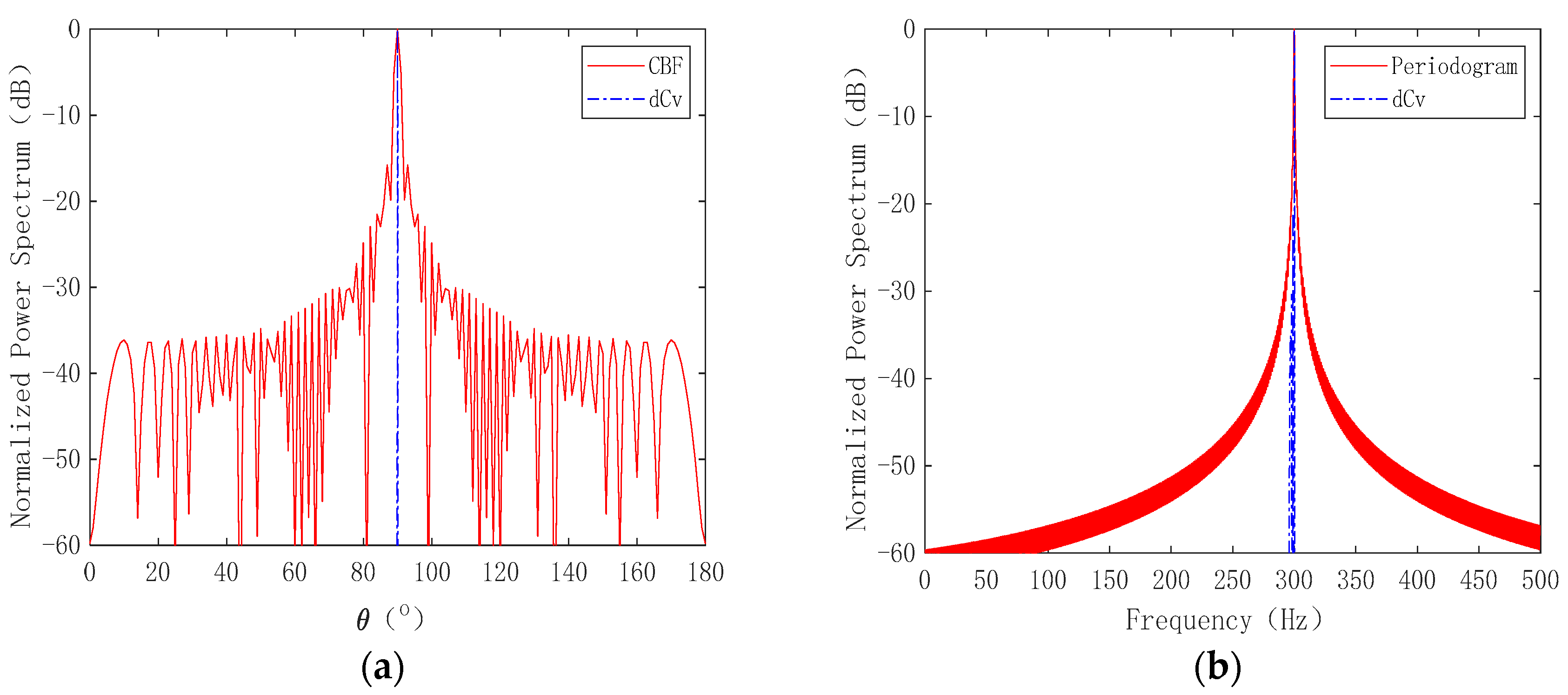
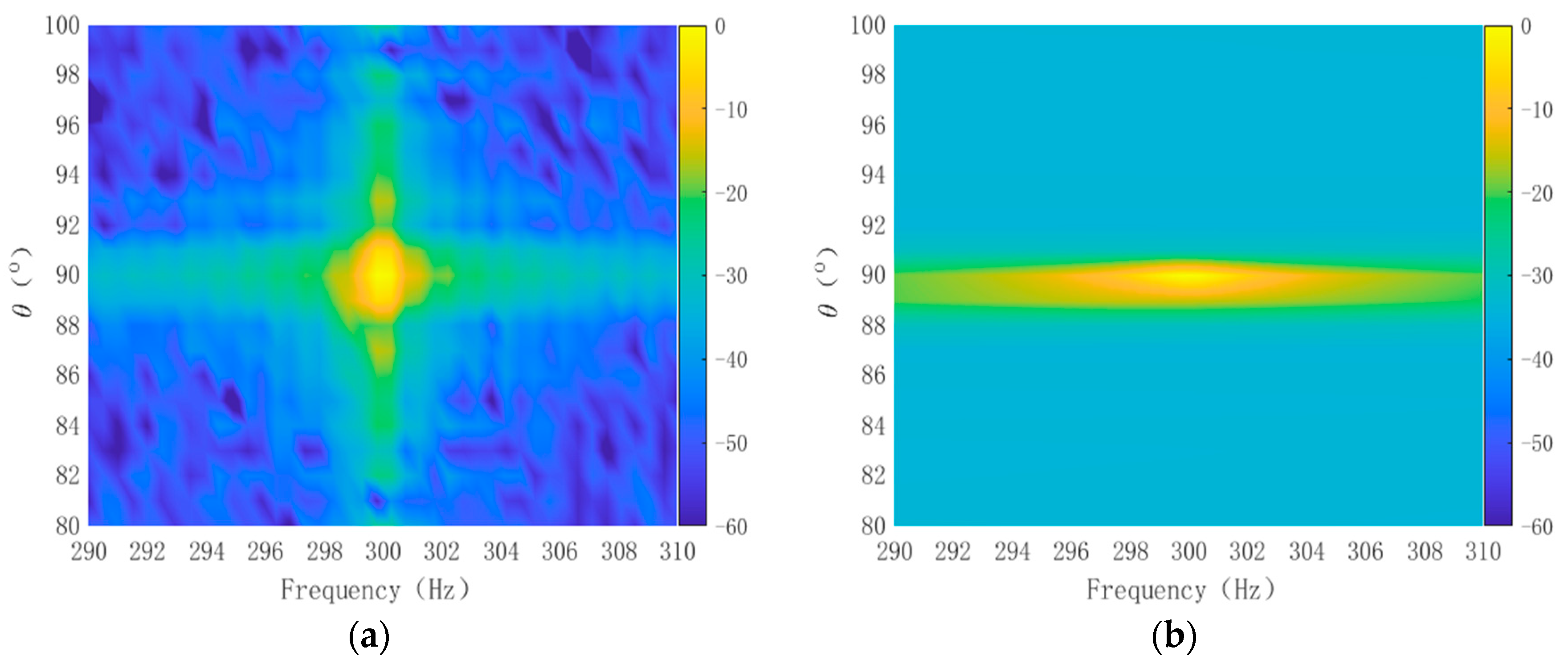
Consider a sinusoidal signal in the far field with a radiation frequency of 300 Hz, an amplitude of 1, and an incidence azimuth of 90°. The duration for signal processing was set at 1.024 s, with a sampling frequency of 1 kHz. Utilizing Equation (8), the relevant azimuth and frequency range were scanned to acquire the FRAZ power spectrum, as depicted in Figure 1a. Additionally, a three-dimensional representation of this spectrum is shown in Figure 1b. These are the original FRAZ spectra obtained directly using frequency–domain beamforming. After undergoing two-dimensional deconvolution processing, the estimated FRAZ spectrum is illustrated in Figure 1c, with its corresponding three-dimensional visualization presented in Figure 1d. These are referred to as the deconvolution FRAZ spectra.
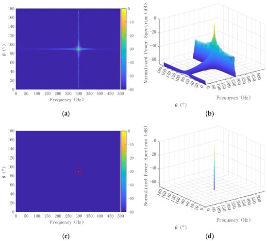
Figure 1.
Results of single target FRAZ spectrum without noise: (a) original FRAZ spectrum; (b) three–dimensional display of original FRAZ spectrum; (c) deconvolution FRAZ spectrum effect; (d) three–dimensional display of deconvolution FRAZ spectrum.
As depicted in Figure 1a,b, the energy of the spatial point source single-frequency signal experienced considerable leakage in both the azimuth and frequency dimensions due to side lobe effects. Figure 1b illustrates that the low-band FRAZ spectrum underwent significant broadening in the azimuth, a consequence of the main lobe width increasing as the frequency decreases. From Figure 1c,d, it is evident that the two-dimensional deconvolution process markedly suppressed side lobes in both the azimuth and frequency dimensions, ideally resolving the issue of energy leakage. The post-deconvolution signal resembled a shock, with the signal energy concentrated solely at the target’s azimuth and frequency. For a meticulous comparative analysis, the azimuth and frequency dimensional slices of the target were individually examined. Figure 2a showcases the azimuth spectrum comparison effect at the frequency point where the target is located, while Figure 2b displays the frequency spectrum comparison effect at the target’s azimuth.
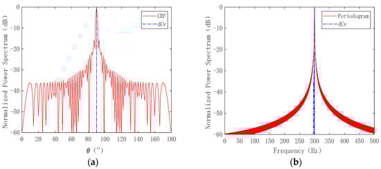
Figure 2.
Comparison of one-dimensional slices of the target: (a) azimuth spectrum comparison; (b) frequency spectrum comparison.
Therefore, in the ideal case without noise, the two-dimensional energy leakage of the frequency–azimuth was ideally suppressed.
3.1.2. Multitarget Estimation with Different SNRs
For evaluating the processing performance of deconvolution FRAZ spectrum estimation, the original FRAZ spectrum estimation was compared with reference algorithms such as 2D-MVDR [4] and 2D-MUSIC [8]. A more complex scenario was considered, involving four point source single-frequency signals in the far field. These signals had incidence angles of 120°, 110°, 90°, and 80° and radiation frequencies of 275 Hz, 300 Hz, 325 Hz, and 350 Hz, respectively. Their signal-to-noise ratios were 15 dB, 5 dB, −5 dB, and −15 dB. The noise was modeled as Gaussian white noise. The basic parameters for frequency–azimuth signal processing remained consistent with those described in Section 3.1.1. Considering the computational cost and estimation effectiveness of the 2D-MVDR and 2D-MUSIC algorithms, the tapped delay line was set to 8. The original FRAZ spectrum is displayed in Figure 3a, the frequency–azimuth spectrum based on 2D-MVDR is illustrated in Figure 3b, the frequency–azimuth spectrum based on 2D-MUSIC is depicted in Figure 3c, and the results of the deconvolution FRAZ spectrum estimation are shown in Figure 3d.
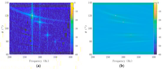
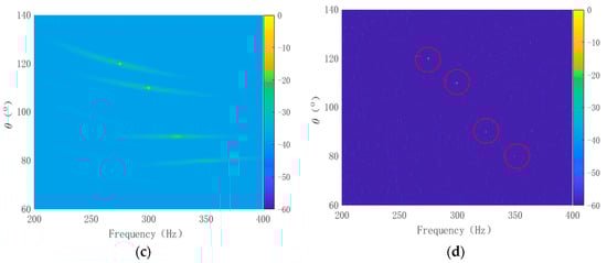
Figure 3.
Multitarget FRAZ spectrum results with different signal-to-noise ratios: (a) original FRAZ spectrum; (b) the 2D-MVDR processing result; (c) the 2D-MUSIC processing result; (d) deconvolution FRAZ spectrum result.
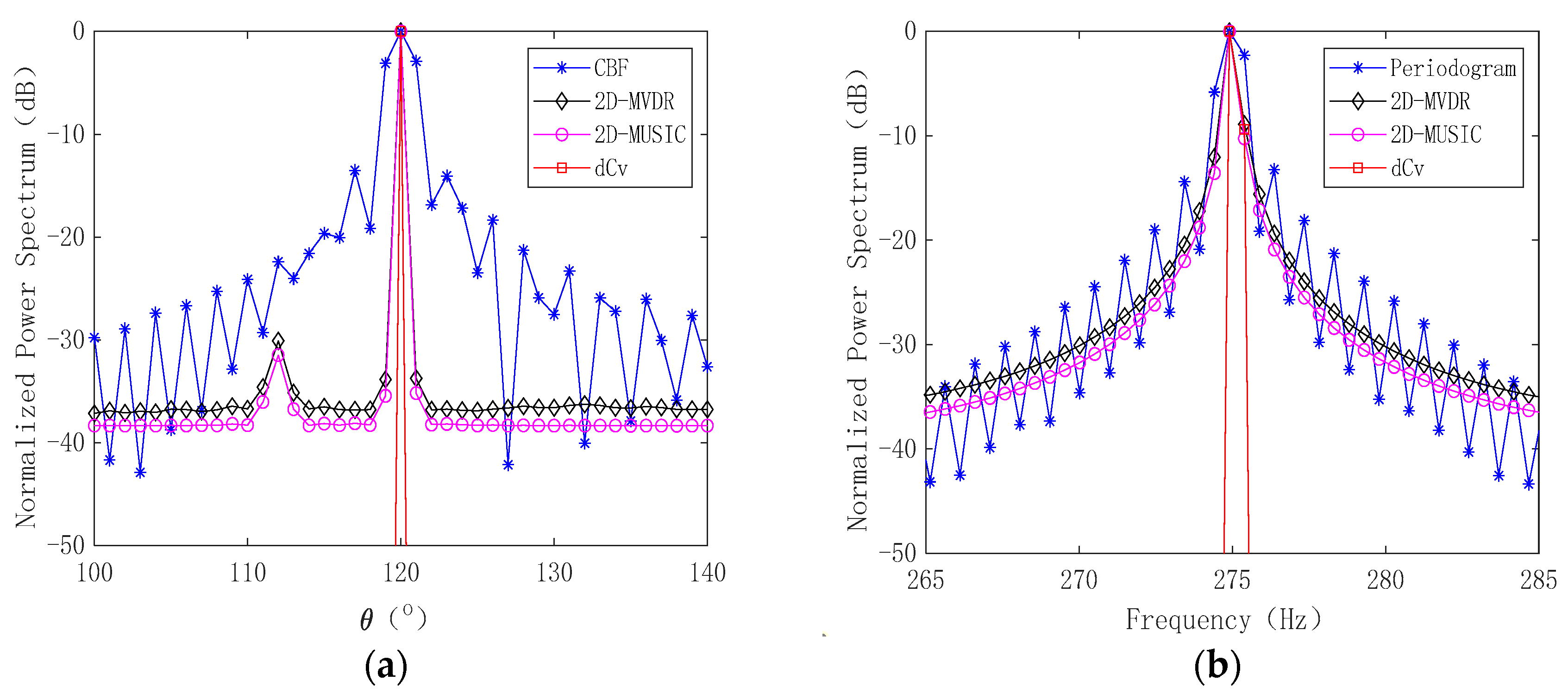
Figure 3 demonstrates that both the 2D-MVDR and 2D-MUSIC methods were effective in reducing energy leakage for the target’s azimuth, compared to the original FRAZ spectrum, although some leakage persisted in the frequency dimension. Notably, the deconvolution-based FRAZ spectrum estimation method proposed in this study proved to be superior in suppressing two-dimensional double-side lobe leakage. A one-dimensional slice of the target located at 120° was selected for detailed examination. Figure 4a presents the azimuth spectrum comparison effect at the target’s frequency point, and Figure 4b shows the spectrum comparison effect at the target’s azimuth.
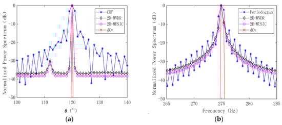
Figure 4.
Comparison of one-dimensional slices of the target: (a) azimuth spectrum comparison; (b) frequency spectrum comparison.
The main lobe of the original FRAZ spectrum was the broadest, and its side lobe was the highest. Compared to this, the main lobe widths in the spectra processed with the 2D-MVDR and 2D-MUSIC algorithms were narrower, and these methods also demonstrated better side lobe suppression than conventional beamforming techniques. The main lobe of the deconvolution FRAZ spectrum, as proposed in this study, was even narrower than those produced by the 2D-MVDR and 2D-MUSIC algorithms. As observed in Figure 4b, since 2D-MVDR and 2D-MUSIC are time-domain processing algorithms, they were less effective in suppressing frequency spectrum leakage. In contrast, the deconvolution FRAZ spectrum estimation algorithm introduced in this paper is a post-processing algorithm based on frequency–domain beamforming, which exhibited a strong capability for spectrum leakage suppression. As demonstrated in Figure 4a,b, the algorithm proposed in this study outperformed the other three algorithms.
The deconvolution gain is calculated according to Equation (23). Each target gain is shown in Table 1.

Table 1.
Deconvolution gain achieved through deconvolution.
The deconvolution gain realized in this study surpassed those reported in References [28,31]. This improvement is attributed to effectively suppressing the two-dimensional energy leakage in the frequency–azimuth domain.
3.1.3. Impact of Iterations on the Deconvolution Gain
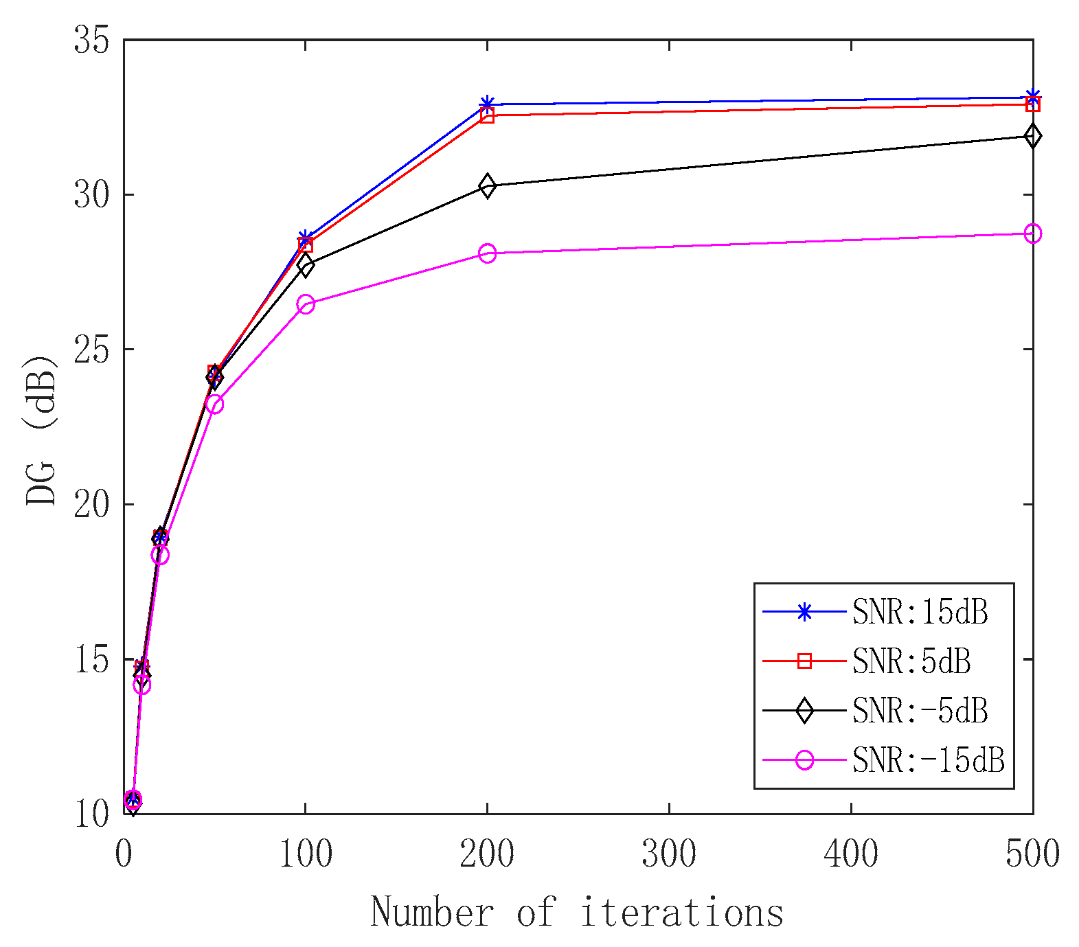
The deconvolution in this study was achieved using the Richardson–Lucy (R–L) algorithm, an iterative process where the number of iterations significantly influences the algorithm’s performance. In the simulation, a sine wave signal was present in the far field, with the radiation frequency matching the array’s center frequency, an incident azimuth of 90°, and the noise characterized as white Gaussian noise. The SNR values were set at 15 dB, 5 dB, −5 dB, and −15 dB. For each SNR condition, the deconvolution iteration parameters were configured for 5, 10, 20, 50, 100, 200, and 500 iterations, respectively. The fundamental parameters for frequency–azimuth signal processing are outlined in Section 3.1.1. Figure 5 illustrates the variation in deconvolution gain with the number of iterations under different SNR conditions.
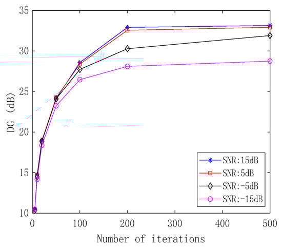
Figure 5.
Deconvolution gain obtained with different SNRs and iterations.
As illustrated in Figure 5, the deconvolution gain improved with an increase in the number of iterations. This enhancement is attributed to the gradual narrowing of the main lobe as the iterations progress, which in turn increases the accuracy of the FRAZ spectrum estimation. However, beyond a certain point, the deconvolution gain tended to stabilize because the iterative algorithm approached convergence. Prior to this convergence, the variation in deconvolution gain across different input SNRs was not substantial.
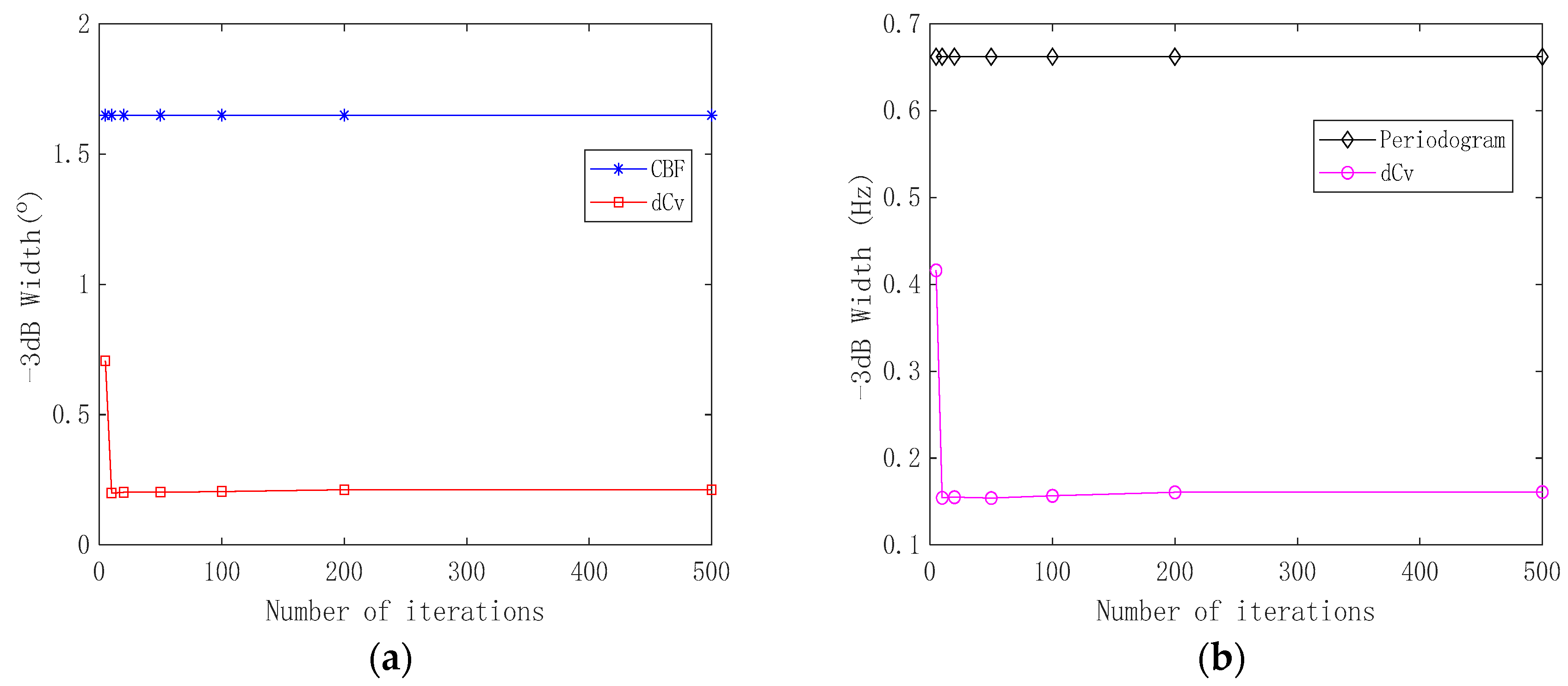
To further elucidate, the half-power beamwidth (i.e., −3 dB width) of the signal spectral peak at a signal-to-noise ratio of 15 dB was calculated. Figure 6a displays the curve of the signal spectral peak −3 dB width in the azimuth dimension as a function of the number of iterations, while Figure 6b presents the curve of the spectral peak −3 dB width in the frequency dimension relative to the number of iterations.
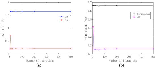
Figure 6.
Comparison of different iterations with −3 dB width: (a) azimuth spectrum main lobe width comparison; (b) frequency spectrum main lobe width comparison.
Figure 6a illustrates that the main lobe width of the azimuth power spectrum decreased as the number of iterations increased. Upon reaching a certain threshold, the main lobe width started to stabilize. Further analysis of Figure 6a,b reveals that post-deconvolution, the azimuth resolution of the line spectrum was significantly enhanced, improving from 1.66° to 0.21°. Similarly, the frequency resolution of the line spectrum was also notably increased, from 0.66 Hz to 0.16 Hz.
3.1.4. Discernability of Adjacent Objects
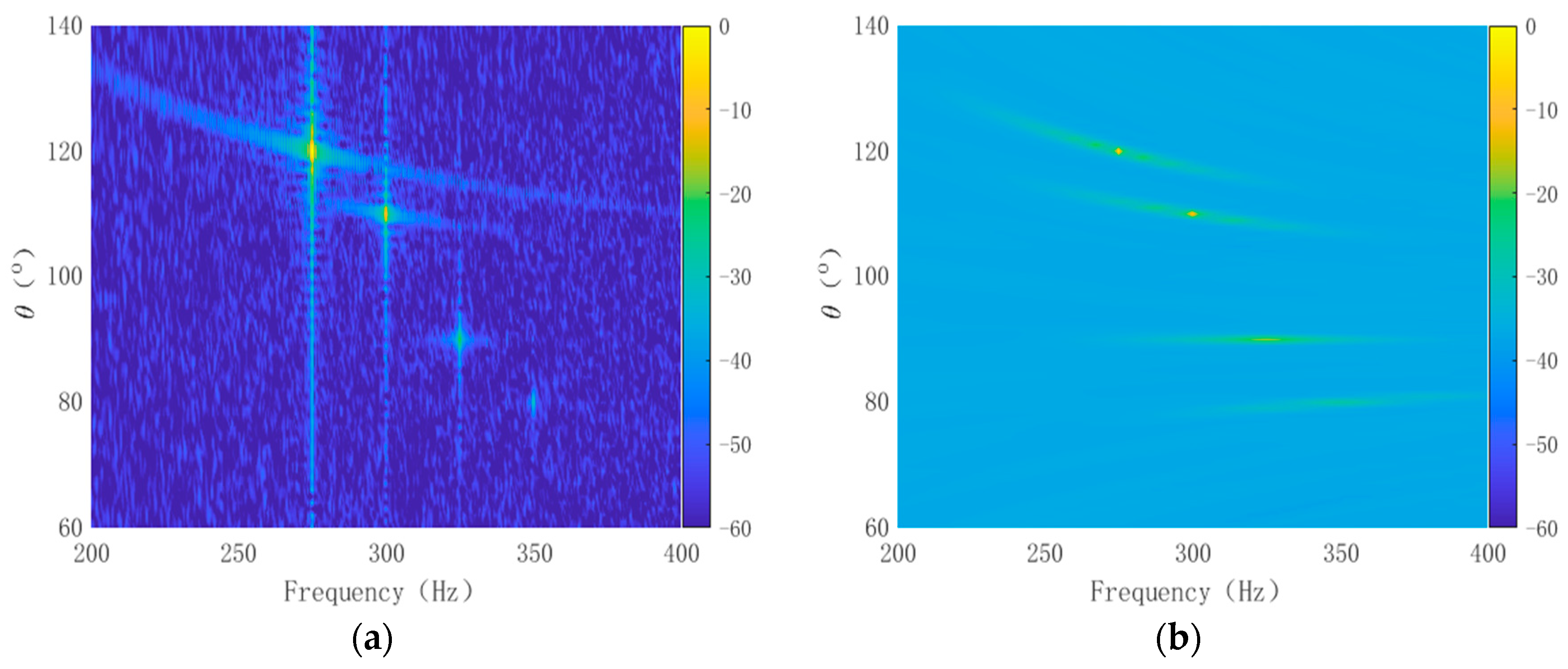
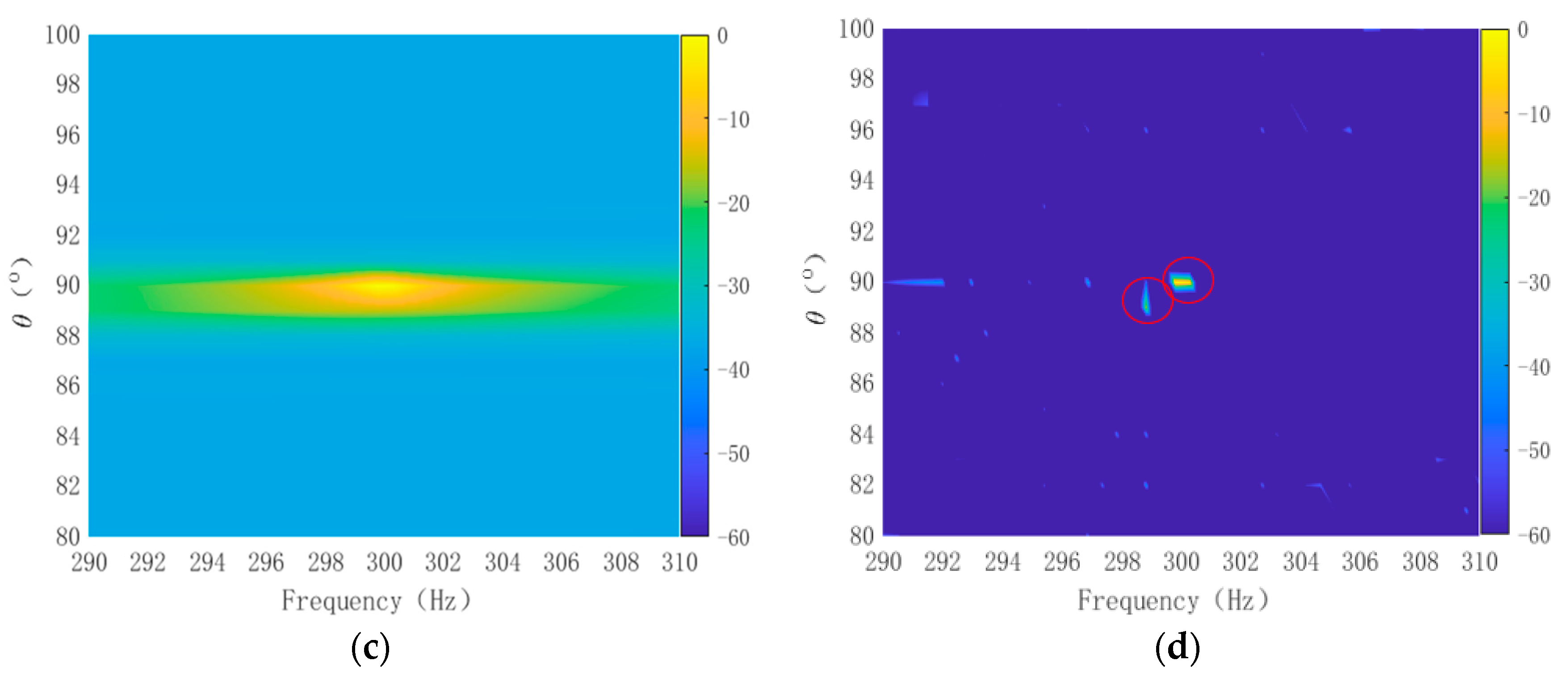
Leveraging the high-resolution property of deconvolution to suppress the side lobes, the impact of two-dimensional deconvolution processing on the resolution of closely spaced, disparate-intensity dual targets was further explored. We considered two adjacent targets: one positioned at an azimuth of 90° with a frequency of 300 Hz and a signal-to-noise ratio (SNR) of 10 dB; the other at an azimuth of 89° with a radiation frequency of 299 Hz and an SNR of −5 dB. The noise remained Gaussian white noise. The basic parameters for frequency–azimuth signal processing were consistent with those detailed in Section 3.1.1. The original FRAZ spectrum is depicted in Figure 7a. It is observable that, due to the low resolution in the frequency and azimuth domains in conventional FRAZ analysis, the strong signal obscured the weak target. Specifically, the azimuth or frequency peak of the weaker signal lay within the side lobe of the stronger signal, rendering the two indistinguishable.
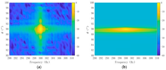

Figure 7.
FRAZ results of adjacent strong and weak targets: (a) original FRAZ spectrum; (b) the 2D-MVDR processing result; (c) the 2D-MUSIC processing result; (d) deconvolution FRAZ spectrum result.
The frequency–azimuth spectra derived from the 2D-MVDR and 2D-MUSIC algorithms are depicted in Figure 7b,c. Due to the inadequate suppression of side lobes in the frequency domain, a one-dimensional masking effect persisted, rendering the two targets indistinct. Conversely, the FRAZ spectrum based on two-dimensional deconvolution is displayed in Figure 7d. The conventional resolution in frequency was approximately 0.98 Hz, and in azimuth space, it was about 1.6°. The two targets were so close in azimuth that they fell within a single conventional resolution element, where the weaker target was obscured by the first side lobe of the stronger target. The frequency proximity of the two objects was nearly equivalent to a conventional resolution element. This illustrates that two-dimensional deconvolution processing can surpass traditional resolution limits.
3.2. Sea Trial Data Verification
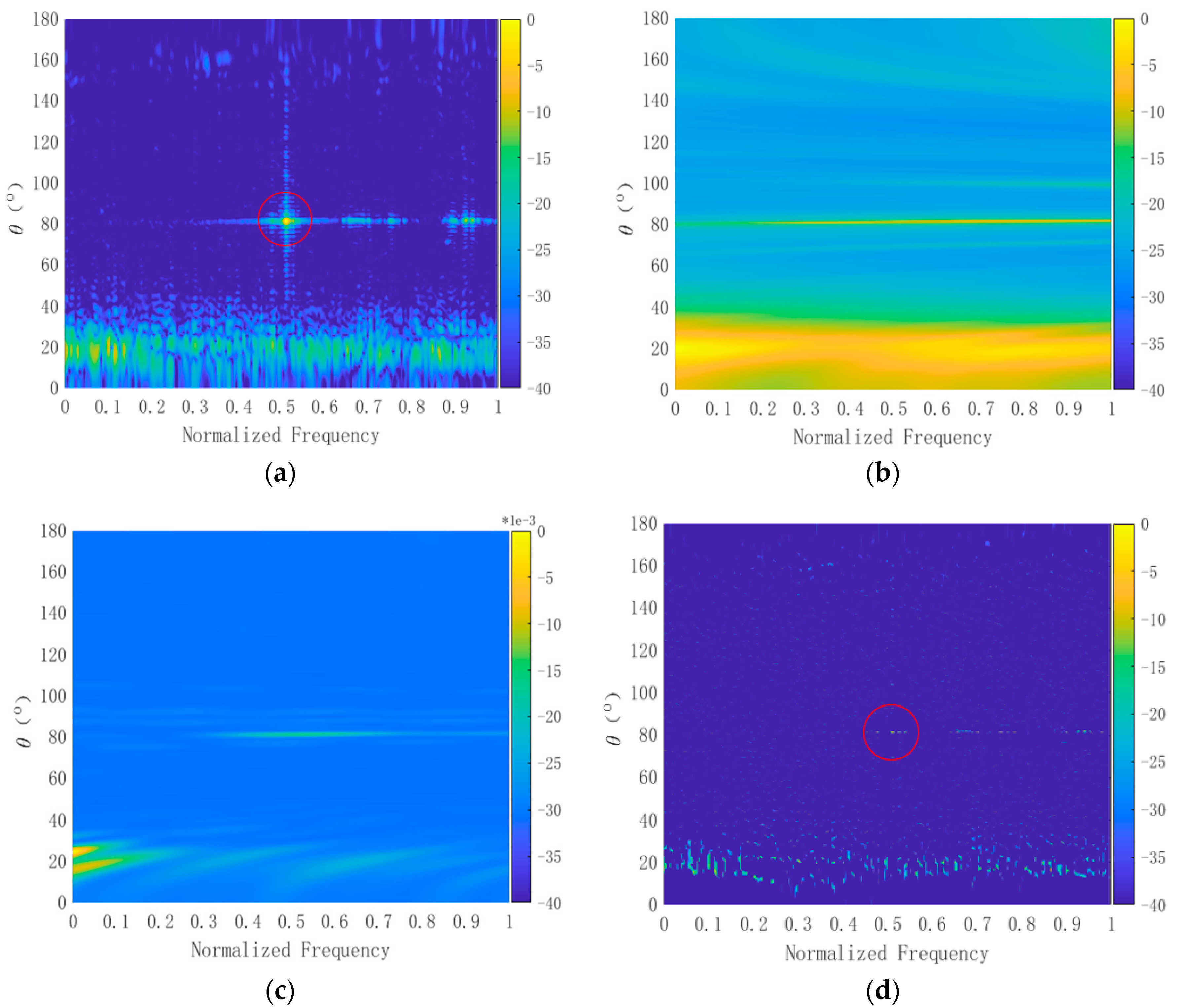
The efficacy of the proposed method was validated using data from a sea trial. This trial involved a passively towed sonar system receiving signals underwater. The shape was a linear array with evenly spaced elements. Notably, there was a sound source exhibiting an intense line spectrum and several weak line spectra near the towline array at an azimuth of 82° and a distance of 22 km. However, the intensity of the source line spectrum and the actual SNR were not determined. Figure 8a presents the FRAZ spectrum obtained through frequency–domain beamforming. Figure 8b,c display the FRAZ spectra acquired using the 2D-MVDR and 2D-MUSIC algorithms, respectively, while Figure 8d showcases the FRAZ spectrum obtained through deconvolution.

Figure 8.
FRAZ results of sea trial data: (a) original FRAZ spectrum; (b) the 2D-MVDR processing results; (c) the 2D-MUSIC processing results; (d) FRAZ spectrum effects after deconvolution.
Figure 8 illustrates that in the original FRAZ spectrum, the line spectrum target exhibited significant leakage in both frequency and azimuth beams, considerably complicating the determination of whether a target possesses a line spectrum. Furthermore, energy leakage across multiple beams severely hinders target interpretation, especially in the case of a single target. It is challenging to capture the target line spectrum and differentiate multiple targets. With the 2D-MVDR processing, the target’s azimuth was observed, but the signal’s frequency information remained elusive. Although the 2D-MUSIC processing offered better estimates of the target azimuth, it still failed to accurately capture the line spectrum, and some of the weaker line spectrum information was lost. The performance of 2D-MVDR and 2D-MUSIC algorithms deteriorated notably when the array position was misaligned, and the number of information sources was unknown. In contrast, the deconvolution FRAZ spectrum successfully captured the main components of the target’s line spectrum with clarity, and these line spectral clusters were distinctly defined at a specific azimuth angle. Despite the presence of other diffuse energy manifestations in Figure 8d that are difficult to interpret, they do not impede the understanding of this source. The scattered energy might originate from an unknown source or unascertained radiation in the test, while the power near a bearing of 20° likely represents the strong self-noise of the tug.
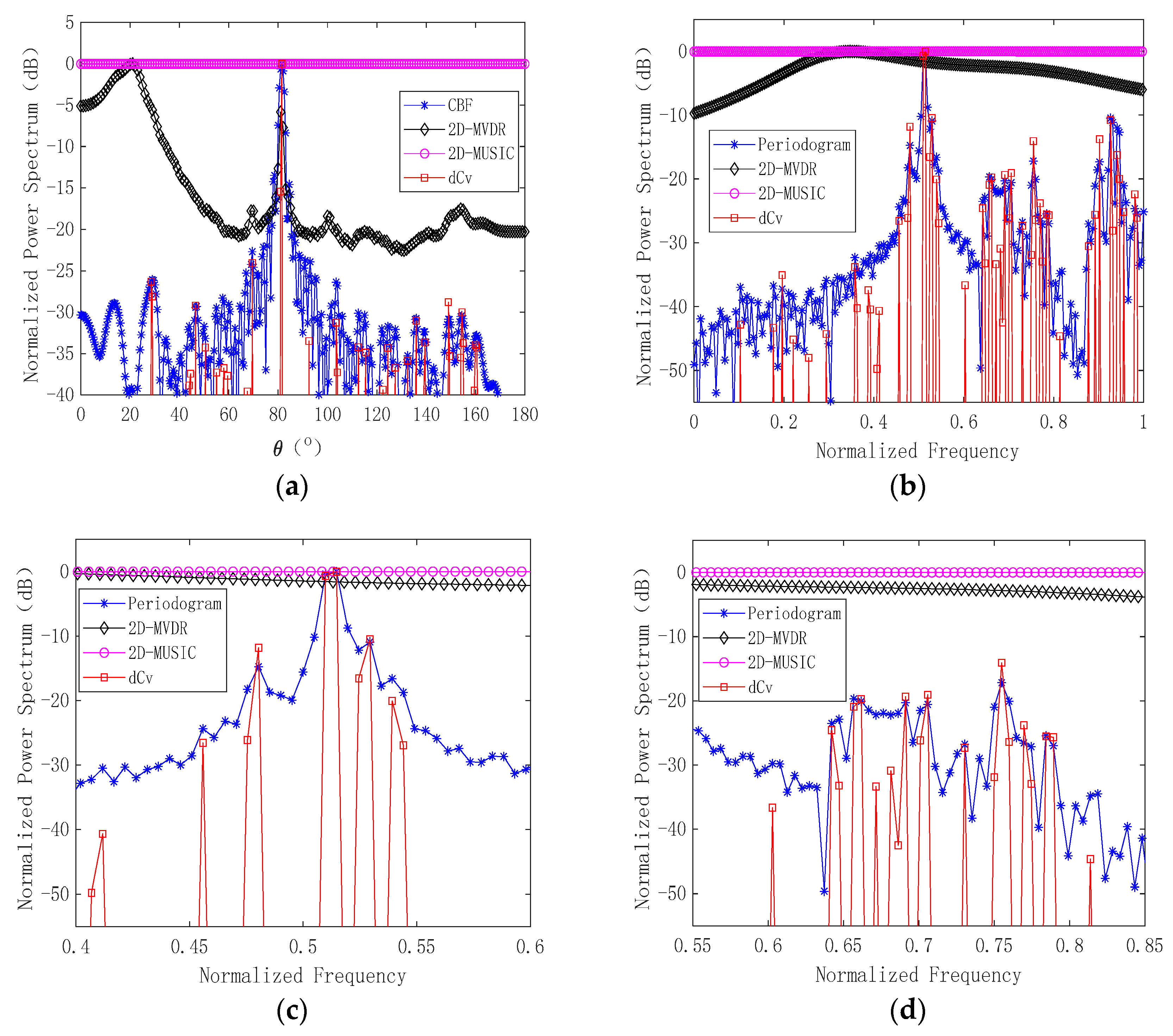
After carefully viewing the one-dimensional slice of the target, the azimuth spectrum comparison effect of the frequency point where the target is located is shown in Figure 9a, and the frequency spectrum comparison effect of the azimuth where the target is located is shown in Figure 9b. The local magnification of Figure 9b is shown in Figure 9c,d.
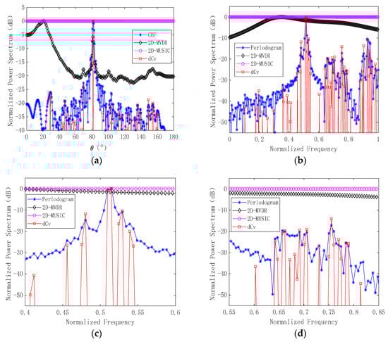
Figure 9.
Comparison of one-dimensional slices of the target: (a) azimuth spectrum comparison; (b) frequency spectrum comparison; (c) local spectrum amplification; (d) local spectrum amplification.
As can be seen from Figure 9, the performance of the 2D-MUSIC algorithm was seriously degraded, the background noise level was significantly improved, and the dynamic range of data was reduced. Compared with other algorithms in the same data dynamic range, the target could not be directly observed. The 2D-MVDR algorithm could keep the target from the azimuth, but there were significant deviations in the signal frequency estimation. The proposed algorithm accurately estimated the target information both in the azimuth and frequency, reduced the side lobe, and restrained the energy leakage in the azimuth and frequency. As seen in Figure 9c, due to the energy leakage of the strong line spectrum, several weak line spectrums are masked by the side lobe of the strong line spectrum. After processing using the algorithm in this paper, the strong and weak line spectrum was distinguished. As seen in Figure 9d, the spectrum obtained using Fourier theory could not distinguish several line spectrums due to the limitation in the processing time length. After deconvolution, some line spectrum information could be clearly distinguished due to the enhancement of the frequency resolution. After calculation, the deconvolution gain obtained by the sound source was 15.50 dB.
4. Discussion
It can be seen from the simulation results and the sea test results that after deconvolution, the main lobe is obviously narrowed, the side lobe is significantly suppressed, and the frequency and azimuth resolution are improved. The main reason is that the deconvolution algorithm reduces the adverse effects caused by undersampling in space and time. Of course, due to the influence of noise, this adverse effect cannot be completely eliminated. In the follow-up research work, we can try to reduce the influence of noise on the deconvolution algorithm.
5. Conclusions
Due to the limitations imposed by the physical aperture of the array and the system’s analysis time, signals are often under sampled in both space and time, constraining the array system’s resolution in azimuth and frequency. To enhance the performance under these spatial–temporal undersampling conditions, a novel uniform linear array FRAZ spectrum estimation method is introduced. This method addresses the coupling relationship between the azimuth and frequency in the FRAZ spectrum by constructing a point scattering function with shift-invariant properties through variable substitution. It then employs the Richardson–Lucy (R–L) iterative algorithm for the deconvolution operation. The efficacy of this proposed method was validated through simulation and sea test data. The results indicate that the FRAZ spectrum post-deconvolution features a narrower main lobe and reduced side lobes. Effectively, this method suppresses signal energy leakage and simultaneously enhances the azimuth and frequency resolution. For a 64-element uniform linear array with an element spacing of 2.5 m and a data processing time of 1.024 s, the width of the azimuth power spectrum’s main lobe can be reduced to approximately 12.5%, and that of the frequency power spectrum’s main lobe can be diminished to about 25%. It should be noted that the R–L algorithm is only applicable to systems where the point scattering function has a shift–invariant property.
Author Contributions
Conceptualization, D.L. and Z.C.; methodology, D.L. and W.G.; software, D.L. and W.G.; validation, D.L. and Z.Y.; formal analysis, D.L. and H.C.; investigation, Z.Y.; resources, Z.Y.; data curation, Z.Y.; writing—original draft preparation, D.L. and H.C.; writing—review and editing, D.L., Z.C., W.G. and Z.Y.; visualization, H.C.; supervision, Z.C.; project administration, Z.Y. All authors have read and agreed to the published version of the manuscript.
Funding
This research received no external funding.
Data Availability Statement
Data are contained within the article.
Acknowledgments
The authors of this article express gratitude to all the staff members who participated in the sea trial conducted in July 2021. Their efforts made it possible to gather reliable experimental data for this study.
Conflicts of Interest
The authors declare no conflicts of interest.
References
- Kazarinov, A.S.; Malyshev, V.N. The Experimental Research of DOA Estimation Based on Difference Co-array Method. In Proceedings of the 2023 IEEE 24th International Conference of Young Professionals in Electron Devices and Materials, Novosibirsk, Russia, 29 June–3 July 2023. [Google Scholar]
- Liu, M.; Qu, S.; Zhao, X. Minimum Variance Distortionless Response—Hanbury Brown and Twiss Sound Source Localization. Appl. Sci. 2023, 13, 6013. [Google Scholar] [CrossRef]
- Wei, S.; Tao, C.G.; Li, L.; Wang, F.; Jiang, D.F. Frequency and DOA joint estimation method based on two-layer compressed sensing. J. Shanghai Norm. Univ. (Nat. Sci.) 2018, 47, 179–185. [Google Scholar]
- Capon, J. High-resolution frequency-wavenumber spectrum analysis. Proc. IEEE 1969, 57, 1408–1418. [Google Scholar] [CrossRef]
- Wang, Y.; Leus, G. Space-time compressive sampling array. In Proceedings of the 2010 IEEE Sensor Array and Multichannel Signal Processing Workshop, Jerusalem, Israel, 4–7 October 2010. [Google Scholar]
- Kim, S.; Lee, K.K. Low-Complexity Joint Extrapolation-MUSIC-Based 2-D Parameter Estimator for Vital FMCW Radar. IEEE Sens. J. 2019, 19, 2205–2216. [Google Scholar] [CrossRef]
- Henninger, M.; Mandelli, S.; Arnold, M.; Brink, S.T. A Computationally Efficient 2D MUSIC Approach for 5G and 6G Sensing Networks. In Proceedings of the 2022 IEEE Wireless Communications and Networking Conference, Austin, TX, USA, 10–13 April 2022. [Google Scholar]
- Xu, Y.G.; Liu, Z.W. Introduction to Array Signal Processing; Beijing Institute of Technology Press: Beijing, China, 2020; pp. 135–139. [Google Scholar]
- Noureddine, L.; Harabi, F.; Gharsallah, A. Space-time estimation algorithms for wideband signals. In Proceedings of the 2015 IEEE 15th Mediterranean Microwave Symposium, Lecce, Italy, 30 November–2 December 2015. [Google Scholar]
- Yin, T. Research on Multi-parameter Estimation in Array Signal. Master’s Thesis, XiDian University, Xi’an, China, 2018. [Google Scholar]
- Lemma, A.N.; van der Veen, A.-J.; Deprettere, E.F. Analysis of joint angle-frequency estimation using ESPRIT. IEEE Trans. Signal Process. 2003, 51, 1264–1283. [Google Scholar] [CrossRef]
- Wen, D.; Yi, H.; Zhang, W.; Xu, H. 2D-Unitary ESPRIT Based Multi-Target Joint Range and Velocity Estimation Algorithm for FMCW Radar. Appl. Sci. 2023, 13, 10448. [Google Scholar] [CrossRef]
- Amanat, A.; Mahmoudi, A.; Hatam, M. Two-dimensional noisy autoregressive estimation with application to joint frequency and direction of arrival estimation. Multidimens. Syst. Signal Process. 2018, 29, 671–685. [Google Scholar] [CrossRef]
- Xu, Y.G.; Liu, Z.W. A New Method for Simultaneous Estimation of Frequency and DOA of Emitters. Acta Electron. Sin. 2001, 09, 1179–1182. [Google Scholar]
- Stein, S.; Yair, O.; Cohen, D.; Eldar, Y.C. Joint Spectrum Sensing and Direction of Arrival Recovery from Sub-Nyquist Samples. In Proceedings of the 2015 IEEE 16th International Workshop on Signal Processing Advances in Wireless Communications, Stockholm, Sweden, 28 June–1 July 2015. [Google Scholar]
- Kumar, A.A.; Razul, S.G.; See, C.-M.S. Carrier Frequency and Direction of Arrival Estimation with Nested Sub-nyquist Sensor Array Receiver. In Proceedings of the 2015 23rd European Signal Processing Conference, Nice, France, 31 August–4 September 2015. [Google Scholar]
- Kumar, A.A.; Chandra, M.G.; Balamuralidhar, P. Joint frequency and 2-D DOA recovery with sub-Nyquist difference space-time array. In Proceedings of the 2017 25th European Signal Processing Conference, Kos, Greece, 28 August–2 September 2017. [Google Scholar]
- Zhang, Z.; Wei, P.; Zhang, H.; Deng, L. Joint spectrum sensing and DOA estimation with sub-Nyquist sampling. Signal Process. 2021, 189, 108260. [Google Scholar] [CrossRef]
- Yang, L.; Li, J.; Chen, F.; Zheng, Z.; Ji, F.; Yu, H. Joint angular-frequency distribution estimation via spatial-temporal sparse sampling and low-rank matrix recovery. Signal Process. 2023, 206, 108918. [Google Scholar] [CrossRef]
- Liu, L.; Zhang, Z.; Wei, P.; Gao, L.; Zhang, H.; Jiang, H.; Du, K. Joint DOA and Frequency Estimation with Spatial and Temporal Sparse Sampling Based on 2-D Covariance Matrix Expansion. IEEE Sens. J. 2023, 3, 22880–22894. [Google Scholar] [CrossRef]
- Wang, Y.L.; Ma, S.L.; Zou, N.; Liang, G. Detection of Unknown Line-spectrum Underwater Target Using Space-time Processing. J. Electron. Inf. Technol. 2019, 41, 1683–1689. [Google Scholar]
- Shi, Y.J.; Piao, H.C.; Guo, J.Y.; Zhang, L. Signal space transform and multidimensional information joint processing for moving target. Acta Acust. 2023, 48, 920–936. [Google Scholar]
- Ye, W. Feature Extraction Method of Target Radiated Noise Based on Space-Time-Frequency Joint Processing. Master’s Thesis, Southeast University, Nanjing, China, 2019. [Google Scholar]
- Liu, S.T.; Huang, J.G. Discrete-Time Signal Processing; Xi’an Jiaotong University Press: Xi’an, China, 2001; pp. 562–566. [Google Scholar]
- Vishnu, P.; Ramalingam, C.S. A method with lower-than-MLE threshold SNR for frequency estimation of multiple sinusoids. Signal Process. 2021, 186, 108128. [Google Scholar] [CrossRef]
- Fan, L.; Qi, G.Q.; Liu, J.Y. Frequency estimator of sinusoid by interpolated DFT method based on maximum sidelobe decay windows. Signal Process. 2021, 186, 108125. [Google Scholar] [CrossRef]
- Yang, T.C. On conventional beamforming and deconvolution. In Proceedings of the OCEANS-2016, Shanghai, China, 10–13 April 2016. [Google Scholar]
- Yang, T.C. Deconvolved conventional beamforming for a horizontal line array. IEEE J. Ocean. Eng. 2017, 43, 160–172. [Google Scholar] [CrossRef]
- Yang, T.C. Deconvolution of decomposed conventional beamforming. J. Acoust. Soc. Am. 2020, 148, 195–201. [Google Scholar] [CrossRef] [PubMed]
- Ma, C.; Sun, D.J.; Mei, J.; Teng, T. Spatiotemporal two-dimensional deconvolution beam imaging technology. Appl. Acoust. 2021, 183, 108310. [Google Scholar] [CrossRef]
- Guo, W.; Piao, S.C.; Yang, T.C.; Guo, J.; Iqbal, K. High-resolution power spectral estimation method using deconvolution. IEEE J. Ocean. Eng. 2019, 45, 489–499. [Google Scholar] [CrossRef]
- Su, X.R.; Miao, Q.Y.; Sun, X.L.; Ren, H.; Ye, L.; Song, K. An Optimal Subspace Deconvolution Algorithm for Robust and High-Resolution Beamforming. Sensors 2022, 22, 2327. [Google Scholar] [CrossRef] [PubMed]


Disclaimer/Publisher’s Note: The statements, opinions and data contained in all publications are solely those of the individual author(s) and contributor(s) and not of MDPI and/or the editor(s). MDPI and/or the editor(s) disclaim responsibility for any injury to people or property resulting from any ideas, methods, instructions or products referred to in the content. |
© 2024 by the authors. Licensee MDPI, Basel, Switzerland. This article is an open access article distributed under the terms and conditions of the Creative Commons Attribution (CC BY) license (https://creativecommons.org/licenses/by/4.0/).