
Estimates of the Land Surface Hydrology from the Community Land Model Version 5 (CLM5) with Three Meteorological Forcing Datasets over China

 , ,
, ,  ,
,  and
and
Abstract
:
1. Introduction
2. Land Surface Model and Forcing Data
2.1. CLM5
2.2. Meteorological Forcing Data
2.3. Experimental Setup
3. Data and Method
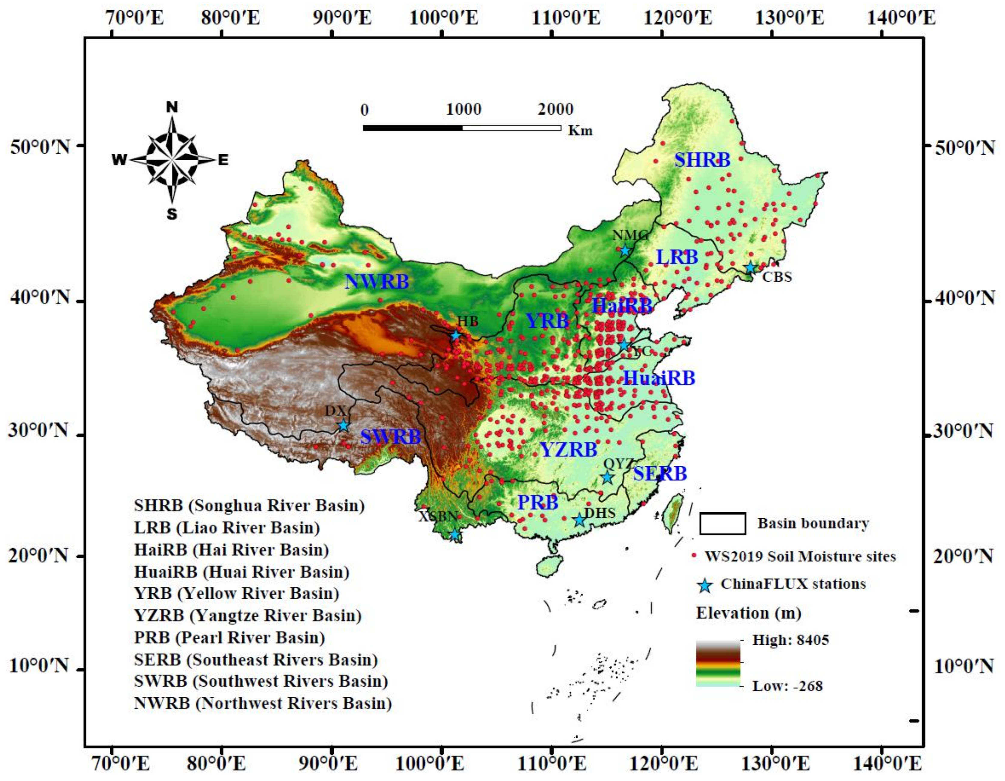
3.1. Validation Data
3.1.1. ET
3.1.2. SM
3.1.3. Runoff
3.2. Evaluation Method
4. Results
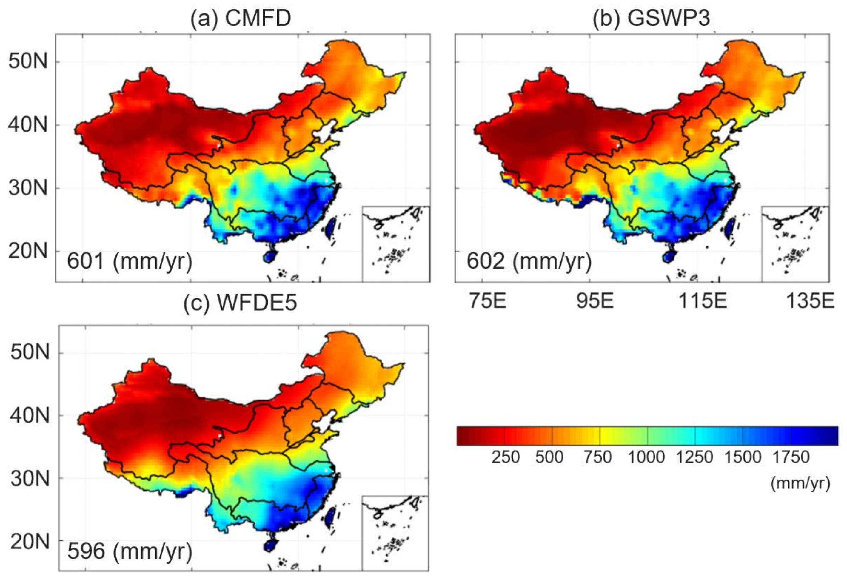
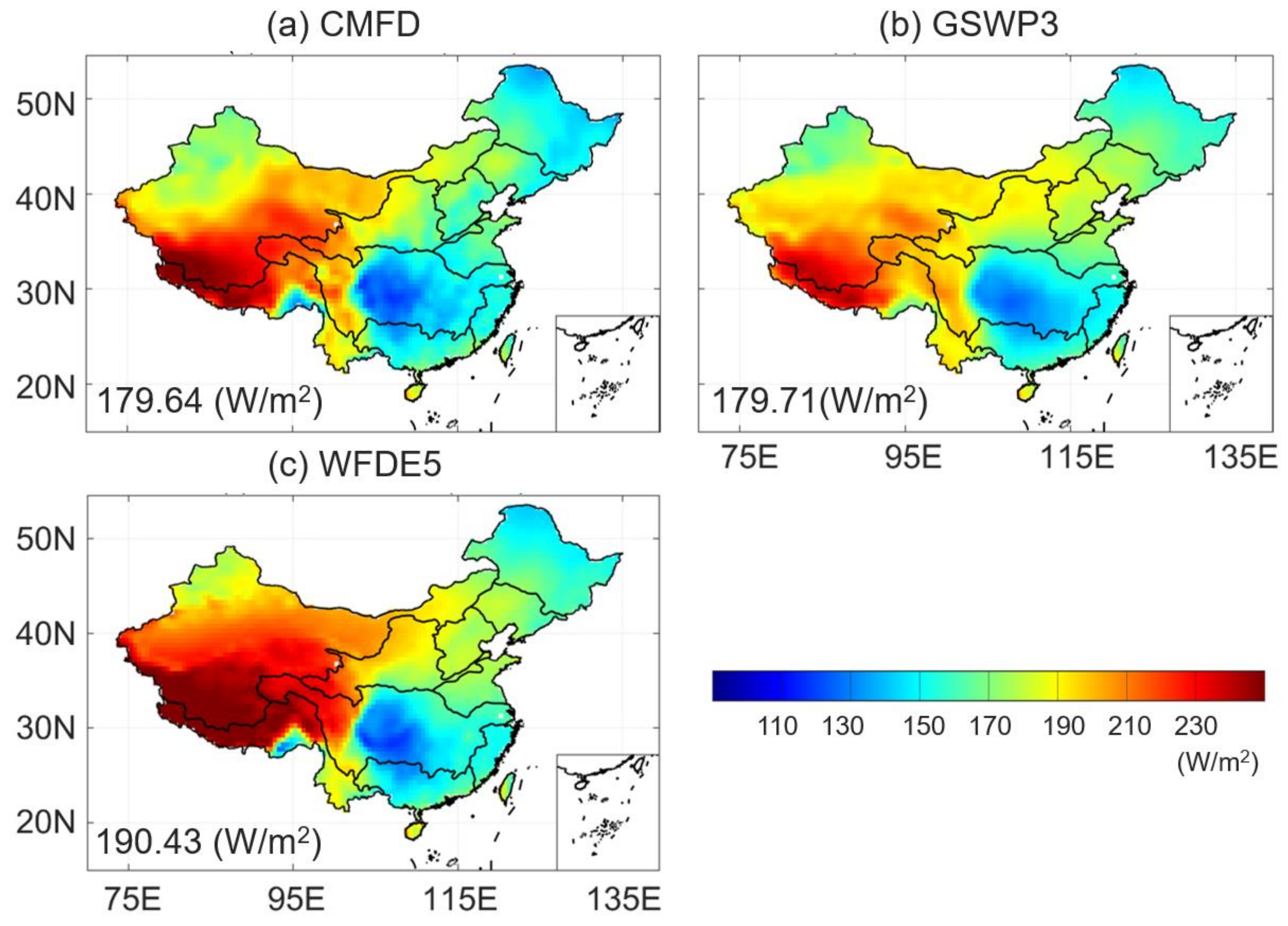
4.1. Intercomparison of Meteorological Forcing Datasets
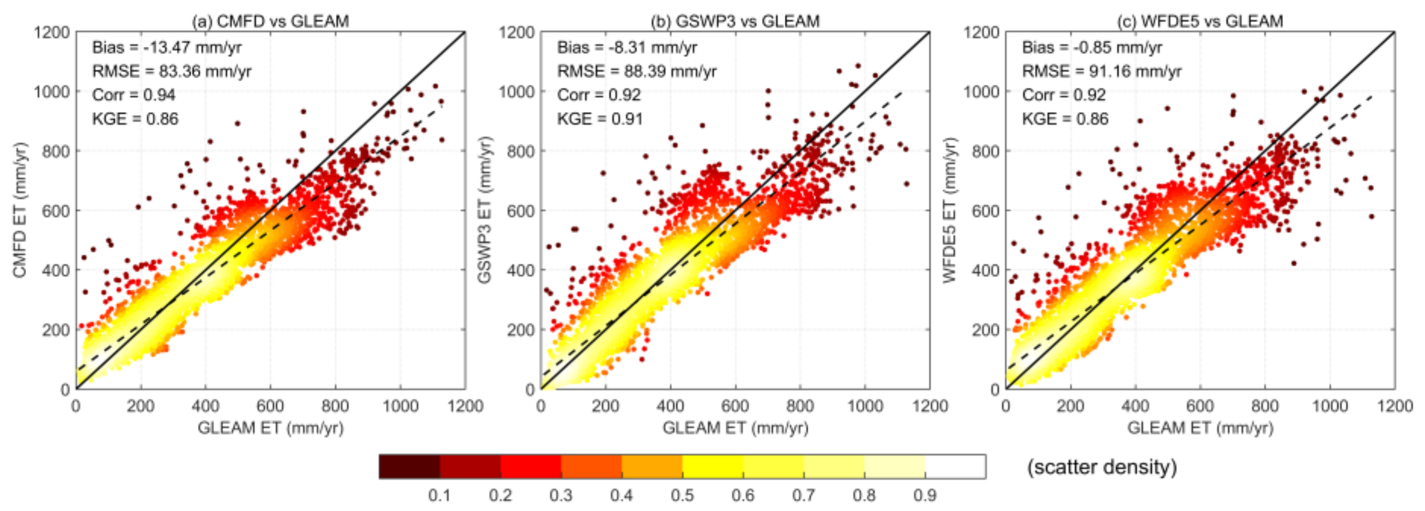
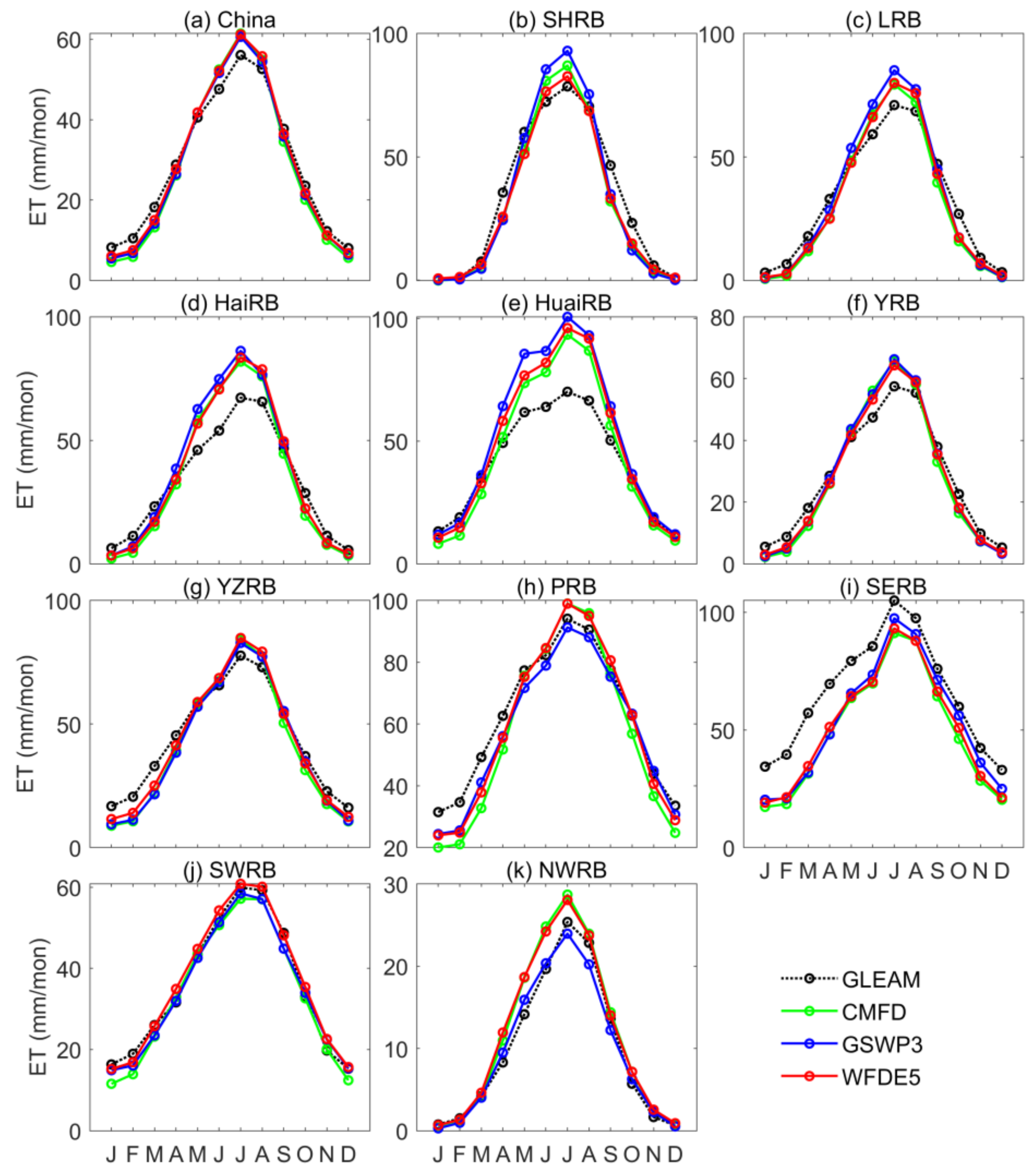
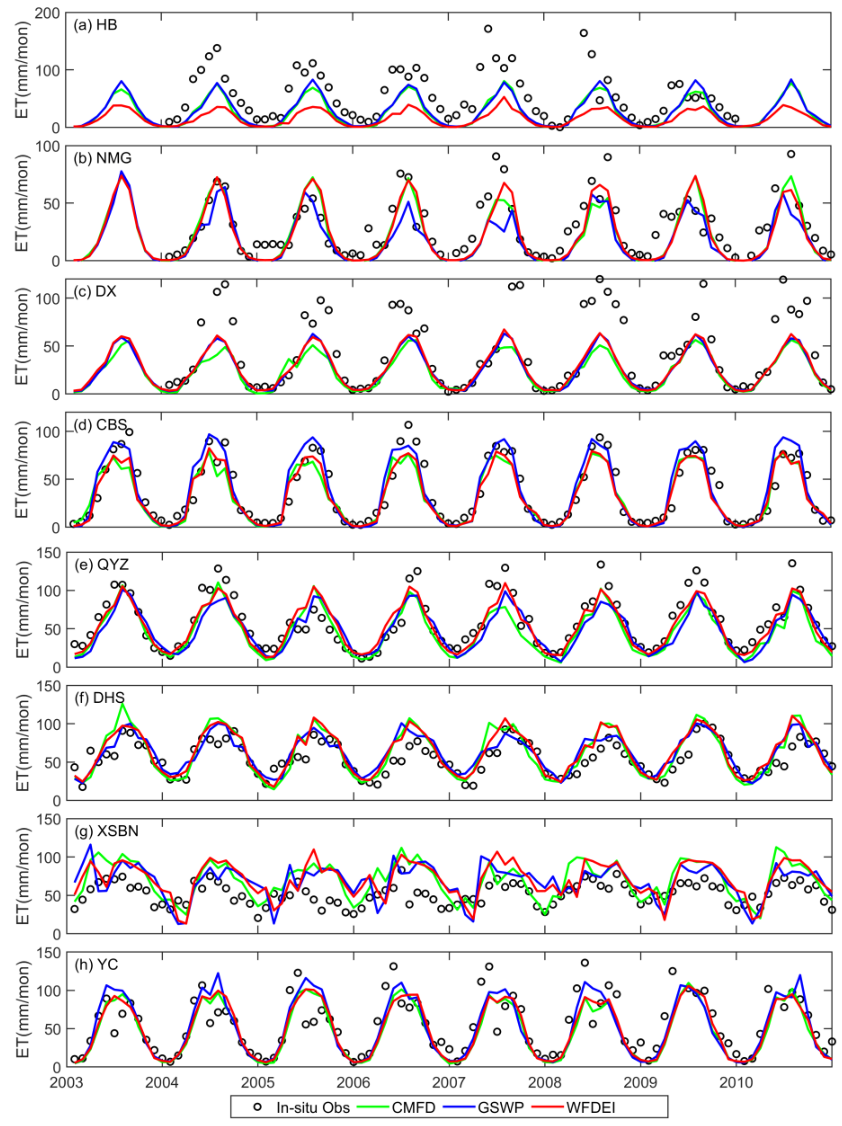
4.2. ET
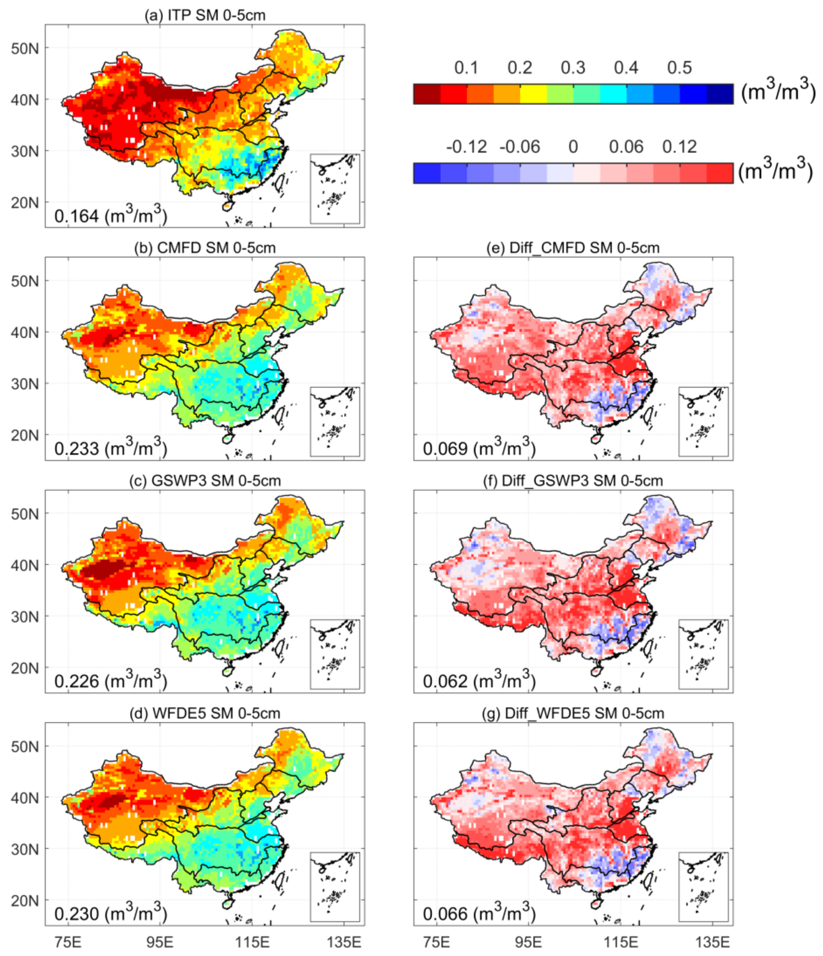
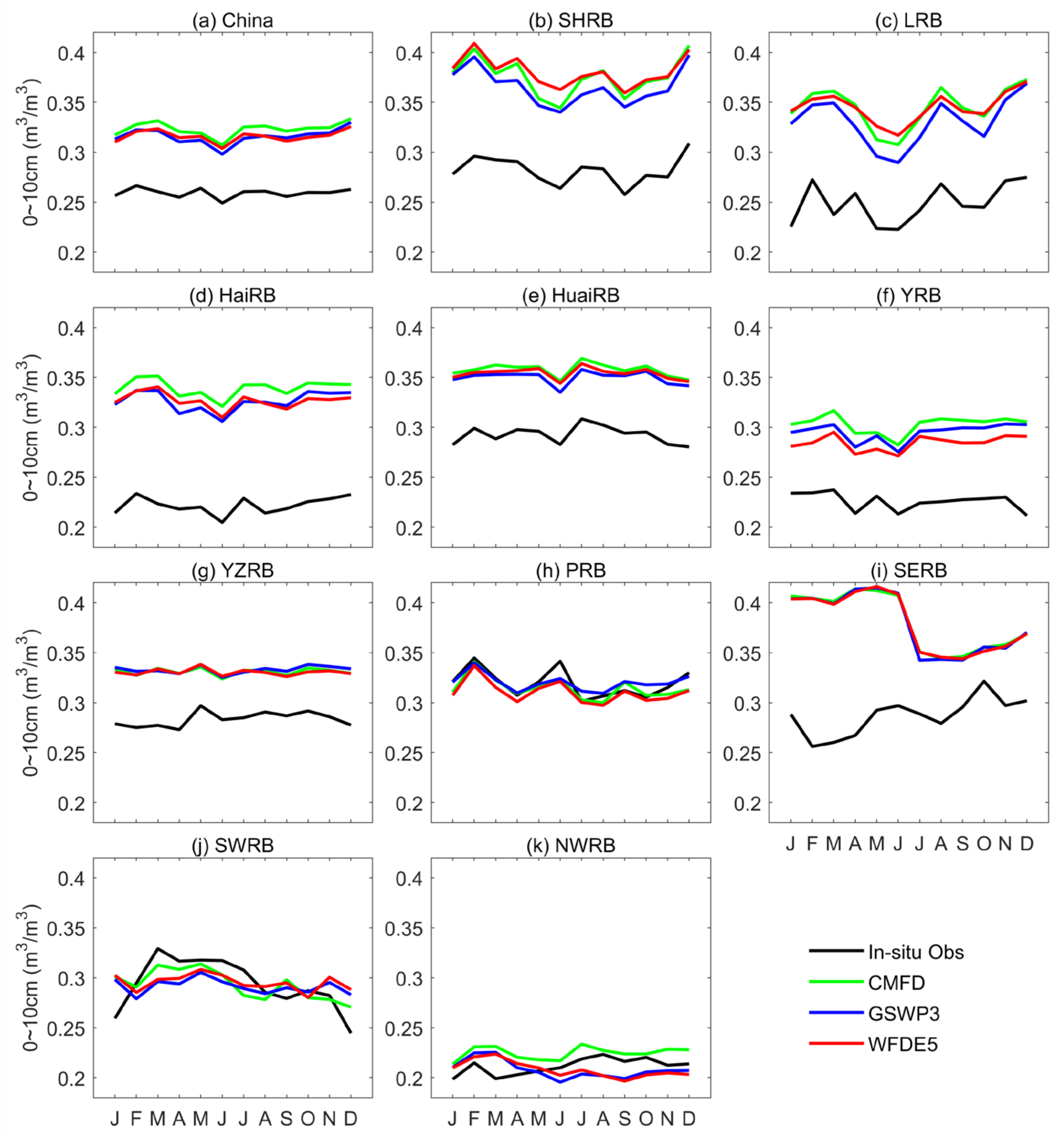
4.3. SM
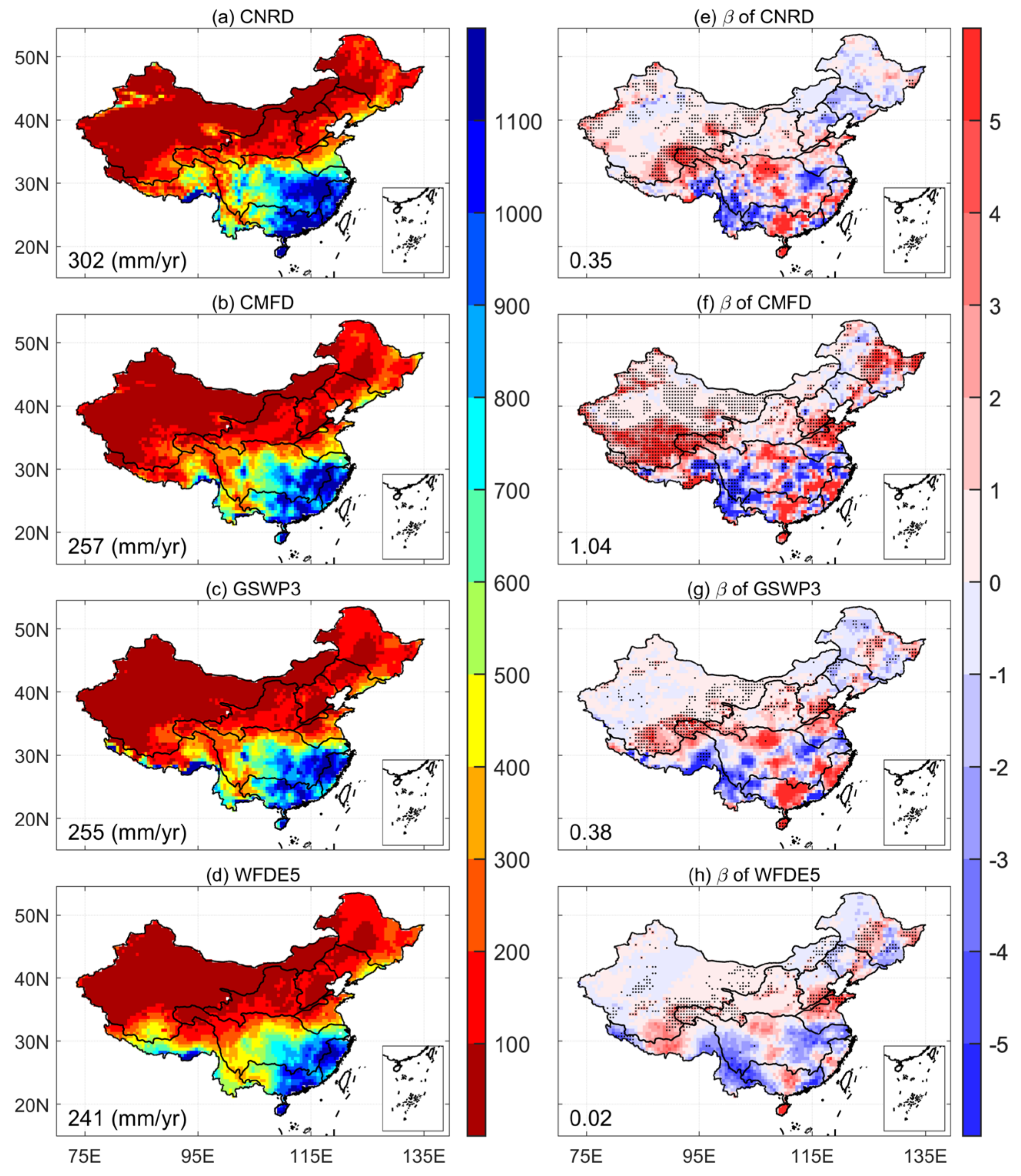
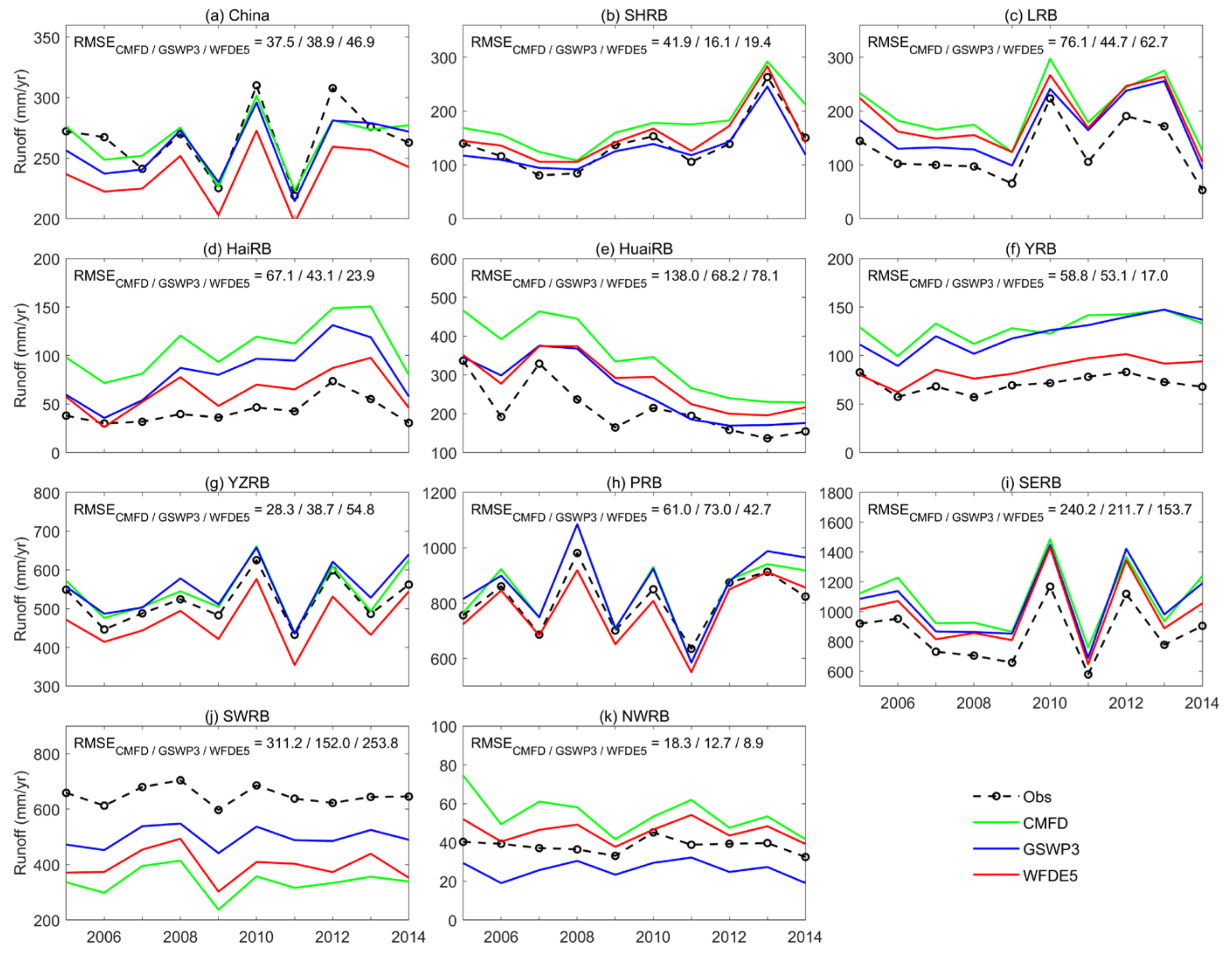
4.4. Runoff
5. Discussion
6. Conclusions
Supplementary Materials
Author Contributions
Funding
Data Availability Statement
Conflicts of Interest
References
- Dickinson, R.E. Land-atmosphere interaction. Rev. Geophys. 1995, 33, 917–922. [Google Scholar] [CrossRef]
- Koster, R.D.; Dirmeyer, P.A.; Guo, Z.; Bonan, G.; Chan, E.; Cox, P.; Gordon, C.T.; Kanae, S.; Kowalczyk, E.; Lawrence, D.; et al. Regions of Strong Coupling Between Soil Moisture and Precipitation. Science 2004, 305, 1138–1140. [Google Scholar] [CrossRef] [PubMed]
- Oleson, K.W.; Niu, G.Y.; Yang, Z.L.; Lawrence, D.M.; Thornton, P.E.; Lawrence, P.J.; Stöckli, R.; Dickinson, R.E.; Bonan, G.B.; Levis, S.; et al. Improvements to the Community Land Model and their impact on the hydrological cycle. J. Geophys. Res. Biogeosci. 2008, 113, 1–26. [Google Scholar] [CrossRef]
- Oki, T.; Kanae, S. Global Hydrological Cycles and World Water Resources. Science 2006, 313, 1068–1072. [Google Scholar] [CrossRef]
- Trenberth, K.E.; Fasullo, J.T.; Kiehl, J. Earth’s Global Energy Budget. Bull. Am. Meteorol. Soc. 2009, 90, 311–324. [Google Scholar] [CrossRef]
- Zhao, M.; Liu, Y.; Konings, A.G. Evapotranspiration frequently increases during droughts. Nat. Clim. Change 2022, 12, 1024–1030. [Google Scholar] [CrossRef]
- Colliander, A.; Reichle, R.H.; Crow, W.T.; Cosh, M.H.; Chen, F.; Chan, S.; Das, N.N.; Bindlish, R.; Chaubell, J.; Kim, S.; et al. Validation of Soil Moisture Data Products from the NASA SMAP Mission. IEEE J. Sel. Top. Appl. Earth Obs. Remote Sens. 2022, 15, 364–392. [Google Scholar] [CrossRef]
- Gao, L.; Gao, Q.; Zhang, H.; Li, X.; Chaubell, M.J.; Ebtehaj, A.; Shen, L.; Wigneron, J.-P. A deep neural network based SMAP soil moisture product. Remote Sens. Environ. 2022, 277, 113059. [Google Scholar] [CrossRef]
- Veldkamp, T.I.E.; Wada, Y.; Aerts, J.C.J.H.; Döll, P.; Gosling, S.N.; Liu, J.; Masaki, Y.; Oki, T.; Ostberg, S.; Pokhrel, Y.; et al. Water scarcity hotspots travel downstream due to human interventions in the 20th and 21st century. Nat. Commun. 2017, 8, 15697. [Google Scholar] [CrossRef]
- Munia, H.A.; Guillaume, J.H.A.; Mirumachi, N.; Wada, Y.; Kummu, M. How downstream sub-basins depend on upstream inflows to avoid scarcity: Typology and global analysis of transboundary rivers. Hydrol. Earth Syst. Sci. 2018, 22, 2795–2809. [Google Scholar] [CrossRef]
- Miao, C.; Gou, J.; Fu, B.; Tang, Q.; Duan, Q.; Chen, Z.; Lei, H.; Chen, J.; Guo, J.; Borthwick, A.G.L.; et al. High-quality reconstruction of China’s natural streamflow. Sci. Bull. 2021, 67, 547–556. [Google Scholar] [CrossRef]
- Bonan, G.B.; Doney, S.C. Climate, ecosystems, and planetary futures: The challenge to predict life in Earth system models. Science 2018, 359, eaam8328. [Google Scholar] [CrossRef]
- Seneviratne, S.I.; Corti, T.; Davin, E.L.; Hirschi, M.; Jaeger, E.B.; Lehner, I.; Orlowsky, B.; Teuling, A.J. Investigating soil moisture–climate interactions in a changing climate: A review. Earth Sci. Rev. 2010, 99, 125–161. [Google Scholar] [CrossRef]
- Wang, D.; Wang, D.; Mo, C. The Use of Remote Sensing-Based ET Estimates to Improve Global Hydrological Simulations in the Community Land Model Version 5.0. Remote Sens. 2021, 13, 4460. [Google Scholar] [CrossRef]
- Wang, A.; Zeng, X.; Guo, D. Estimates of Global Surface Hydrology and Heat Fluxes from the Community Land Model (CLM4.5) with Four Atmospheric Forcing Datasets. J. Hydrometeorol. 2016, 17, 2493–2510. [Google Scholar] [CrossRef]
- Chen, Y.; Yuan, H. Evaluation of nine sub-daily soil moisture model products over China using high-resolution in situ observations. J. Hydrol. 2020, 588, 125054. [Google Scholar] [CrossRef]
- Lawrence, D.M.; Fisher, R.A.; Koven, C.D.; Oleson, K.W.; Swenson, S.C.; Bonan, G.; Collier, N.; Ghimire, B.; Kampenhout, L.; Kennedy, D.; et al. The Community Land Model Version 5: Description of New Features, Benchmarking, and Impact of Forcing Uncertainty. J. Adv. Model. Earth Syst. 2019, 11, 4245–4287. [Google Scholar] [CrossRef]
- Fisher, R.A.; Koven, C.D. Perspectives on the Future of Land Surface Models and the Challenges of Representing Complex Terrestrial Systems. J. Adv. Model. Earth Syst. 2020, 12, e2018MS001453. [Google Scholar] [CrossRef]
- Cherkauer, K.A.; Lettenmaier, D.P. Hydrologic effects of frozen soils in the upper Mississippi River basin. J. Geophys. Res. Atmos. 1999, 104, 19599–19610. [Google Scholar] [CrossRef]
- Andreadis, K.M.; Storck, P.; Lettenmaier, D.P. Modeling snow accumulation and ablation processes in forested environments. Water Resour. Res. 2009, 45, 1–13. [Google Scholar] [CrossRef]
- Hamman, J.J.; Nijssen, B.; Bohn, T.J.; Gergel, D.R.; Mao, Y.X. The Variable Infiltration Capacity model version 5 (VIC-5): Infrastructure improvements for new applications and reproducibility. Geosci. Model Dev. 2018, 11, 3481–3496. [Google Scholar] [CrossRef]
- Ghimire, B.; Riley, W.J.; Koven, C.D.; Mu, M.; Randerson, J.T. Representing leaf and root physiological traits in CLM improves global carbon and nitrogen cycling predictions. J. Adv. Model. Earth Syst. 2016, 8, 598–613. [Google Scholar] [CrossRef]
- van Kampenhout, L.; Lenaerts, J.T.M.; Lipscomb, W.H.; Sacks, W.J.; Lawrence, D.M.; Slater, A.G.; van den Broeke, M.R. Improving the Representation of Polar Snow and Firn in the Community Earth System Model. J. Adv. Model. Earth Syst. 2017, 9, 2583–2600. [Google Scholar] [CrossRef]
- Blyth, E.M.; Arora, V.K.; Clark, D.B.; Dadson, S.J.; De Kauwe, M.G.; Lawrence, D.M.; Melton, J.R.; Pongratz, J.; Turton, R.H.; Yoshimura, K.; et al. Advances in Land Surface Modelling. Curr. Clim. Change Rep. 2021, 7, 45–71. [Google Scholar] [CrossRef]
- Ou, M.; Zhang, S. Evaluation and Comparison of the Common Land Model and the Community Land Model by Using In Situ Soil Moisture Observations from the Soil Climate Analysis Network. Land 2022, 11, 126. [Google Scholar] [CrossRef]
- Yokohata, T.; Kinoshita, T.; Sakurai, G.; Pokhrel, Y.; Ito, A.; Okada, M.; Satoh, Y.; Kato, E.; Nitta, T.; Fujimori, S.; et al. MIROC-INTEG-LAND version 1: A global biogeochemical land surface model with human water management, crop growth, and land-use change. Geosci. Model Dev. 2020, 13, 4713–4747. [Google Scholar] [CrossRef]
- Song, J.; Miller, G.R.; Cahill, A.T.; Aparecido, L.M.T.; Moore, G.W. Modeling land surface processes over a mountainous rainforest in Costa Rica using CLM4.5 and CLM5. Geosci. Model Dev. 2020, 13, 5147–5173. [Google Scholar] [CrossRef]
- Cheng, Y.; Huang, M.; Zhu, B.; Bisht, G.; Zhou, T.; Liu, Y.; Song, F.; He, X. Validation of the Community Land Model Version 5 Over the Contiguous United States (CONUS) Using In Situ and Remote Sensing Data Sets. J. Geophys. Res. Atmos. 2021, 126, e2020JD033539. [Google Scholar] [CrossRef]
- Parr, D.; Wang, G.; Bjerklie, D. Integrating Remote Sensing Data on Evapotranspiration and Leaf Area Index with Hydrological Modeling: Impacts on Model Performance and Future Predictions. J. Hydrometeorol. 2015, 16, 2086–2100. [Google Scholar] [CrossRef]
- Wang, D.; Wang, G.; Parr, D.T.; Liao, W.; Xia, Y.; Fu, C. Incorporating remote sensing-based ET estimates into the Community Land Model version 4.5. Hydrol. Earth Syst. Sci. 2017, 21, 3557–3577. [Google Scholar] [CrossRef]
- Yang, S.; Li, R.; Wu, T.; Wu, X.; Zhao, L.; Hu, G.; Zhu, X.; Du, Y.; Xiao, Y.; Zhang, Y.; et al. Evaluation of soil thermal conductivity schemes incorporated into CLM5.0 in permafrost regions on the Tibetan Plateau. Geoderma 2021, 401, 115330. [Google Scholar] [CrossRef]
- Cucchi, M.; Weedon, G.P.; Amici, A.; Bellouin, N.; Lange, S.; Müller Schmied, H.; Hersbach, H.; Buontempo, C. WFDE5: Bias-adjusted ERA5 reanalysis data for impact studies. Earth Syst. Sci. Data 2020, 12, 2097–2120. [Google Scholar] [CrossRef]
- Wang, A.; Zeng, X. Sensitivities of terrestrial water cycle simulations to the variations of precipitation and air temperature in China. J. Geophys. Res. 2011, 116, 1–11. [Google Scholar] [CrossRef]
- Liu, J.; Shi, C.; Sun, S.; Liang, J.; Yang, Z.-L. Improving Land Surface Hydrological Simulations in China Using CLDAS Meteorological Forcing Data. J. Meteorol. Res. 2020, 33, 1194–1206. [Google Scholar] [CrossRef]
- Tesfa, T.K.; Li, H.Y.; Leung, L.R.; Huang, M.; Ke, Y.; Sun, Y.; Liu, Y. A subbasin-based framework to represent land surface processes in an Earth system model. Geosci. Model Dev. 2014, 7, 947–963. [Google Scholar] [CrossRef]
- Shi, C.; Jiang, L.; Zhang, T.; Xu, B.; Han, S. Status and Plans of CMA Land Data Assimilation System (CLDAS) Project. EGU Gen. Assem. 2014, 16, EGU2014-5671. [Google Scholar]
- He, J.; Yang, K.; Tang, W.; Lu, H.; Qin, J.; Chen, Y.; Li, X. The first high-resolution meteorological forcing dataset for land process studies over China. Sci. Data 2020, 7, 25. [Google Scholar] [CrossRef] [PubMed]
- Liu, J.G.; Xie, Z.H. Improving simulation of soil moisture in China using a multiple meteorological forcing ensemble approach. Hydrol. Earth Syst. Sci. 2013, 17, 3355–3369. [Google Scholar] [CrossRef]
- Lin, X.; Zhang, H.; Zhang, X.-j.; Liu, J.; Chen, J.; Shao, Q.; Chen, B.; Sun, S. Modeling Evapotranspiration over China’s Landmass from 1979 to 2012 Using Multiple Land Surface Models: Evaluations and Analyses. J. Hydrometeorol. 2017, 18, 1185–1203. [Google Scholar]
- Lu, H.; Zheng, D.; Yang, K.; Yang, F. Last-decade progress in understanding and modeling the land surface processes on the Tibetan Plateau. Hydrol. Earth Syst. Sci. 2020, 24, 5745–5758. [Google Scholar] [CrossRef]
- Liu, J.; Yang, Z.-L.; Jia, B.; Wang, L.; Wang, P.; Xie, Z.; Shi, C. Elucidating Dominant Factors Affecting Land Surface Hydrological Simulations of the Community Land Model over China. Adv. Atmos. Sci. 2022, 40, 235–250. [Google Scholar] [CrossRef]
- Ma, X.; Wang, A. Systematic Evaluation of a High-Resolution CLM5 Simulation over Continental China for 1979–2018. J. Hydrometeorol. 2022, 23, 1879–1897. [Google Scholar] [CrossRef]
- Bonan, G.B. The land surface climatology of the NCAR land surface model coupled to the NCAR community climate model. J. Clim. 1998, 11, 1307–1326. [Google Scholar] [CrossRef]
- Zhao, F.; Wang, X.; Wu, Y.; Singh, S.K. Prefectures vulnerable to water scarcity are not evenly distributed across China. Commun. Earth Environ. 2023, 4, 145. [Google Scholar] [CrossRef]
- Hanasaki, N.; Oki, T.; Guo, Z.; Zhao, M.; Gao, X.; Dirmeyer, P.A. GSWP-2: Multimodel Analysis and Implications for Our Perception of the Land Surface. Bull. Am. Meteorol. Soc. 2006, 87, 1381–1398. [Google Scholar]
- Hou, Y.; Guo, H.; Yang, Y.; Liu, W. Global Evaluation of Runoff Simulation from Climate, Hydrological and Land Surface Models. Water Resour. Res. 2022, 59, e2021WR031817. [Google Scholar] [CrossRef]
- Gou, J.; Miao, C.; Samaniego, L.; Xiao, M.; Wu, J.; Guo, X. CNRD v1.0: A High-Quality Natural Runoff Dataset for Hydrological and Climate Studies in China. Bull. Am. Meteorol. Soc. 2021, 102, E929–E947. [Google Scholar] [CrossRef]
- Lawrence, D.M.; Thornton, P.E.; Oleson, K.W.; Bonan, G.B. The Partitioning of Evapotranspiration into Transpiration, Soil Evaporation, and Canopy Evaporation in a GCM: Impacts on Land–Atmosphere Interaction. J. Hydrometeorol. 2007, 8, 862–880. [Google Scholar] [CrossRef]
- Miralles, D.G.; Holmes, T.R.H.; De Jeu, R.A.M.; Gash, J.H.; Meesters, A.G.C.A.; Dolman, A.J. Global land-surface evaporation estimated from satellite-based observations. Hydrol. Earth Syst. Sci. 2011, 15, 453–469. [Google Scholar] [CrossRef]
- Martens, B.; Miralles, D.G.; Lievens, H.; van der Schalie, R.; de Jeu, R.A.M.; Fernández-Prieto, D.; Beck, H.E.; Dorigo, W.A.; Verhoest, N.E.C. GLEAM v3: Satellite-based land evaporation and root-zone soil moisture. Geosci. Model Dev. 2017, 10, 1903–1925. [Google Scholar] [CrossRef]
- Bai, P.; Liu, X. Intercomparison and evaluation of three global high-resolution evapotranspiration products across China. J. Hydrol. 2018, 566, 743–755. [Google Scholar] [CrossRef]
- Zhu, W.; Tian, S.; Wei, J.; Jia, S.; Song, Z. Multi-scale evaluation of global evapotranspiration products derived from remote sensing images: Accuracy and uncertainty. J. Hydrol. 2022, 611, 127982. [Google Scholar] [CrossRef]
- Yao, T.; Lu, H.; Yu, Q.; Feng, S.; Xue, Y.; Feng, W. Uncertainties of three high-resolution actual evapotranspiration products across China: Comparisons and applications. Atmos. Res. 2023, 286, 106682. [Google Scholar] [CrossRef]
- Jia, Y.; Li, C.; Yang, H.; Yang, W.; Liu, Z. Assessments of three evapotranspiration products over China using extended triple collocation and water balance methods. J. Hydrol. 2022, 614 Pt B, 128594. [Google Scholar] [CrossRef]
- Yin, L.; Tao, F.; Chen, Y.; Liu, F.; Hu, J. Improving terrestrial evapotranspiration estimation across China during 2000–2018 with machine learning methods. J. Hydrol. 2021, 600, 126538. [Google Scholar] [CrossRef]
- Li, X.; Zou, L.; Xia, J.; Dou, M.; Li, H.; Song, Z. Untangling the effects of climate change and land use/cover change on spatiotemporal variation of evapotranspiration over China. J. Hydrol. 2022, 612, 128189. [Google Scholar] [CrossRef]
- Bai, P. Comparison of remote sensing evapotranspiration models: Consistency, merits, and pitfalls. J. Hydrol. 2023, 617, 128856. [Google Scholar] [CrossRef]
- Yang, K.; Chen, Y.; He, J.; Zhao, L.; Lu, H.; Qin, J.; Zheng, D.; Li, X. Development of a daily soil moisture product for the period of 2002–2011 in Chinese mainland. Sci. China Earth Sci. 2020, 63, 1113–1125. [Google Scholar] [CrossRef]
- Yang, K.; Zhu, L.; Chen, Y.; Zhao, L.; Qin, J.; Lu, H.; Tang, W.; Han, M.; Ding, B.; Fang, N. Land surface model calibration through microwave data assimilation for improving soil moisture simulations. J. Hydrol. 2016, 533, 266–276. [Google Scholar] [CrossRef]
- Wang, A.; Shi, X. A Multilayer Soil Moisture Dataset Based on the Gravimetric Method in China and Its Characteristics. J. Hydrometeorol. 2019, 20, 1721–1736. [Google Scholar] [CrossRef]
- Sang, Y.; Ren, H.-L.; Shi, X.; Xu, X.; Chen, H. Improvement of Soil Moisture Simulation in Eurasia by the Beijing Climate Center Climate System Model from CMIP5 to CMIP6. Adv. Atmos. Sci. 2021, 38, 237–252. [Google Scholar] [CrossRef]
- Peng, D.; Zhou, Q.; Tang, X.; Yan, W.; Chen, M. Changes in soil moisture caused solely by vegetation restoration in the karst region of southwest China. J. Hydrol. 2022, 613, 128460. [Google Scholar] [CrossRef]
- Zhou, Y.; Chen, H.; Sun, S. Assessing and comparing the subseasonal variations of summer soil moisture of satellite products over eastern China. Int. J. Climatol. 2023, 43, 3925–3946. [Google Scholar] [CrossRef]
- Gou, J.; Miao, C.; Duan, Q.; Tang, Q.; Di, Z.; Liao, W.; Wu, J.; Zhou, R. Sensitivity Analysis-Based Automatic Parameter Calibration of the VIC Model for Streamflow Simulations Over China. Water Resour. Res. 2020, 56, e2019WR025968. [Google Scholar] [CrossRef]
- Mann, H.B. Nonparametric tests against trend. Econometrica 1945, 13, 245–259. [Google Scholar] [CrossRef]
- Sen, P.K. Estimates of the Regression Coefficient Based on Kendall’s Tau. J. Am. Stat. Assoc. 1968, 63, 1379–1389. [Google Scholar] [CrossRef]
- Zhao, R.; Wang, H.; Chen, J.; Fu, G.; Zhan, C.; Yang, H. Quantitative analysis of nonlinear climate change impact on drought based on the standardized precipitation and evapotranspiration index. Ecol. Indic. 2021, 121, 107107. [Google Scholar] [CrossRef]
- Deng, M.; Meng, X.; Lyv, Y.; Zhao, L.; Li, Z.; Hu, Z.; Jing, H. Comparison of Soil Water and Heat Transfer Modeling Over the Tibetan Plateau Using Two Community Land Surface Model (CLM) Versions. J. Adv. Model. Earth Syst. 2020, 12, e2020MS002189. [Google Scholar] [CrossRef]
- Fatichi, S.; Or, D.; Walko, R.; Vereecken, H.; Young, M.H.; Ghezzehei, T.A.; Hengl, T.; Kollet, S.; Agam, N.; Avissar, R. Soil structure is an important omission in Earth System Models. Nat. Commun. 2020, 11, 522. [Google Scholar] [CrossRef]
- Sun, R.; Duan, Q.; Wang, J. Understanding the spatial patterns of evapotranspiration estimates from land surface models over China. J. Hydrol. 2021, 595, 126021. [Google Scholar] [CrossRef]
- Kumar, S.; Holmes, T.; Mocko, D.M.; Wang, S.; Peters-Lidard, C. Attribution of flux partitioning variations between land surface models over the continental U.S. Remote Sens. 2018, 10, 751. [Google Scholar] [CrossRef]
- Cheng, Y.; Ogden, F.L.; Zhu, J. Characterization of sudden and sustained base flow jump hydrologic behaviour in the humid seasonal tropics of the Panama Canal Watershed. Hydrol. Process. 2019, 34, 569–582. [Google Scholar] [CrossRef]
- Cheng, Y.; Ogden, F.L.; Zhu, J.; Bretfeld, M. Land Use-Dependent Preferential Flow Paths Affect Hydrological Response of Steep Tropical Lowland Catchments with Saprolitic Soils. Water Resour. Res. 2018, 54, 5551–5566. [Google Scholar] [CrossRef]
- Hou, Z.; Huang, M.; Leung, L.R.; Lin, G.; Ricciuto, D.M. Sensitivity of surface flux simulations to hydrologic parameters based on an uncertainty quantification framework applied to the Community Land Model. J. Geophys. Res. Atmos. 2012, 117, 1–18. [Google Scholar] [CrossRef]
- Ren, H.; Hou, Z.; Huang, M.; Bao, J.; Sun, Y.; Tesfa, T.; Ruby Leung, L. Classification of hydrological parameter sensitivity and evaluation of parameter transferability across 431 US MOPEX basins. J. Hydrol. 2016, 536, 92–108. [Google Scholar] [CrossRef]
- Gong, W.; Duan, Q.; Li, J.; Wang, C.; Di, Z.; Ye, A.; Miao, C.; Dai, Y. Multiobjective adaptive surrogate modeling-based optimization for parameter estimation of large, complex geophysical models. Water Resour. Res. 2016, 52, 1984–2008. [Google Scholar] [CrossRef]
- Xia, Y.; Mocko, D.M.; Wang, S.; Pan, M.; Kumar, S.V.; Peters-Lidard, C.D.; Wei, H.; Wang, D.; Ek, M.B. Comprehensive Evaluation of the Variable Infiltration Capacity (VIC) Model in the North American Land Data Assimilation System. J. Hydrometeorol. 2018, 19, 1853–1879. [Google Scholar] [CrossRef]
- Xu, T.; Guo, Z.; Xia, Y.; Ferreira, V.G.; Liu, S.; Wang, K.; Yao, Y.; Zhang, X.; Zhao, C. Evaluation of twelve evapotranspiration products from machine learning, remote sensing and land surface models over conterminous United States. J. Hydrol. 2019, 578, 124105. [Google Scholar] [CrossRef]
- Baez-Villanueva, O.M.; Zambrano-Bigiarini, M.; Beck, H.E.; McNamara, I.; Ribbe, L.; Nauditt, A.; Birkel, C.; Verbist, K.; Giraldo-Osorio, J.D.; Thinh, N.X. RF-MEP: A novel random forest method for merging gridded precipitation products and ground-based measurements. Remote Sens. Environ. 2020, 239, 111606. [Google Scholar] [CrossRef]
- Wei, L.; Jiang, S.; Ren, L.; Yuan, S.; Liu, Y.; Yang, X.; Wang, M.; Zhang, L.; Yu, H.; Duan, Z. An extended triple collocation method with maximized correlation for near global land precipitation fusion. Geophys. Res. Lett. 2023, 50, 2023GL105120. [Google Scholar] [CrossRef]


| Sites | Elevation (m) | Ecosystem Type | P (mm/yr) | T (°C) | AI |
|---|---|---|---|---|---|
| HB | 3250 | Alpine meadow | 535 | −1.7 | 1.29 |
| NMG | 1189 | Temperate steppe | 1493 | −0.4 | 2.26 |
| DX | 4333 | Alpine steppe-meadow | 450 | 6.5 | 1.73 |
| CBS | 738 | Temperate mixed forest | 713 | 3.6 | 0.79 |
| QYZ | 102 | Subtropical planted coniferous forest | 1542 | 17.9 | 0.72 |
| DHS | 300 | South subtropical evergreen broadleaved forest | 1956 | 21.0 | 0.67 |
| XSBN | 750 | Tropic seasonal rainforest | 1493 | 21.8 | 0.80 |
| YC | 28 | Temperate farmland | 582 | 13.1 | 1.78 |
| Elements | CMFD | GSWP3 | WFDE5 |
|---|---|---|---|
| Precipitation (mm/yr) | 601 | 602 | 596 |
| Solar radiation (W/m2) | 179.64 | 179.71 | 190.43 |
| Downward longwave radiation (W/m2) | 284.08 | 287.03 | 278.98 |
| Air temperature (°C) | 6.44 | 7.07 | 7.01 |
| Humidity (kg/kg) | 0.006 | 0.006 | 0.006 |
| Wind speed (m/s) | 2.45 | 2.48 | 2.65 |
| Surface pressure (kPa) | 83.76 | 83.29 | 83.26 |
| Regions | Simulations | Bias (mm/yr) | RB (%) | RMSE (mm/yr) | Corr | KGE |
|---|---|---|---|---|---|---|
| China | CMFD | −13.5 | 18.8 | 83.4 | 0.94 | 0.86 |
| GSWP3 | −8.3 | 3.6 | 88.4 | 0.92 | 0.91 | |
| WFDE5 | −0.8 | 23.5 | 91.2 | 0.92 | 0.86 | |
| SHRB | CMFD | −33.7 | −4.2 | 72.7 | 0.35 | 0.29 |
| GSWP3 | −11.9 | 1.1 | 70.8 | 0.36 | 0.35 | |
| WFDE5 | −36.3 | −4.8 | 77.1 | 0.29 | 0.24 | |
| LRB | CMFD | −24.7 | −5.2 | 50.9 | 0.82 | 0.75 |
| GSWP3 | 9.2 | 2.7 | 44.8 | 0.85 | 0.84 | |
| WFDE5 | −13.3 | −2.2 | 49.5 | 0.79 | 0.75 | |
| HaiRB | CMFD | 15.6 | 4.5 | 76.3 | 0.44 | 0.17 |
| GSWP3 | 51.0 | 13.3 | 106.9 | 0.40 | −0.05 | |
| WFDE5 | 34.6 | 9.4 | 104.3 | 0.33 | −0.16 | |
| HuaiRB | CMFD | 51.1 | 12.7 | 91.6 | 0.38 | 0.36 |
| GSWP3 | 133.3 | 29.5 | 159.9 | 0.39 | 0.34 | |
| WFDE5 | 93.5 | 21.3 | 124.9 | 0.38 | 0.35 | |
| YRB | CMFD | −10.8 | −0.4 | 60.5 | 0.82 | 0.82 |
| GSWP3 | −0.9 | 2.7 | 63.7 | 0.80 | 0.80 | |
| WFDE5 | −6.5 | 0.7 | 66.7 | 0.80 | 0.77 | |
| YZRB | CMFD | −43.3 | −5.0 | 102.4 | 0.78 | 0.71 |
| GSWP3 | −36.2 | −3.6 | 103 | 0.76 | 0.72 | |
| WFDE5 | −17.4 | −0.6 | 100.4 | 0.75 | 0.74 | |
| PRB | CMFD | −65.2 | −7.4 | 117.1 | 0.55 | 0.54 |
| GSWP3 | −49.1 | −5.6 | 120.2 | 0.58 | 0.46 | |
| WFDE5 | −31.1 | −2.6 | 106.6 | 0.50 | 0.50 | |
| SERB | CMFD | −192.3 | −23.0 | 220.5 | −0.04 | −0.12 |
| GSWP3 | −142.7 | −16.8 | 172 | 0.24 | 0.14 | |
| WFDE5 | −168.6 | −20.0 | 197.3 | 0.09 | 0.00 | |
| SWRB | CMFD | −24.7 | 4.2 | 98.5 | 0.96 | 0.79 |
| GSWP3 | −12.1 | 10.7 | 117.5 | 0.94 | 0.71 | |
| WFDE5 | 10.0 | 21.2 | 137.5 | 0.91 | 0.62 | |
| NWRB | CMFD | 18.6 | 55.8 | 56.2 | 0.77 | 0.65 |
| GSWP3 | −1.9 | 5.5 | 57.8 | 0.78 | 0.75 | |
| WFDE5 | 19.5 | 60.1 | 65.2 | 0.70 | 0.60 |
| Regions | Simulations | Bias (m3/m3) | RB (%) | RMSE (m3/m3) | Corr | KGE |
|---|---|---|---|---|---|---|
| China | CMFD | 0.069 | 72.6 | 0.094 | 0.75 | 0.40 |
| GSWP3 | 0.062 | 61.7 | 0.093 | 0.73 | 0.47 | |
| WFDE5 | 0.066 | 69.3 | 0.095 | 0.73 | 0.42 | |
| SHRB | CMFD | 0.030 | 17.6 | 0.069 | 0.23 | 0.18 |
| GSWP3 | 0.017 | 11.8 | 0.071 | 0.10 | 0.03 | |
| WFDE5 | 0.032 | 19.3 | 0.070 | 0.19 | 0.16 | |
| LRB | CMFD | 0.047 | 30.5 | 0.070 | 0.61 | 0.42 |
| GSWP3 | 0.040 | 27.3 | 0.068 | 0.55 | 0.40 | |
| WFDE5 | 0.051 | 33.1 | 0.075 | 0.54 | 0.37 | |
| HaiRB | CMFD | 0.097 | 62.9 | 0.123 | −0.39 | −0.49 |
| GSWP3 | 0.095 | 62.3 | 0.124 | −0.40 | −0.51 | |
| WFDE5 | 0.092 | 60.5 | 0.123 | −0.45 | −0.55 | |
| HuaiRB | CMFD | 0.161 | 87.6 | 0.166 | 0.07 | −0.32 |
| GSWP3 | 0.155 | 84.8 | 0.161 | 0.09 | −0.28 | |
| WFDE5 | 0.159 | 86.8 | 0.165 | 0.05 | −0.32 | |
| YRB | CMFD | 0.091 | 61.8 | 0.103 | 0.54 | 0.25 |
| GSWP3 | 0.094 | 63.5 | 0.107 | 0.53 | 0.22 | |
| WFDE5 | 0.081 | 56.4 | 0.098 | 0.37 | 0.17 | |
| YZRB | CMFD | 0.066 | 35.5 | 0.097 | 0.53 | 0.29 |
| GSWP3 | 0.072 | 38.8 | 0.103 | 0.47 | 0.22 | |
| WFDE5 | 0.068 | 36.7 | 0.100 | 0.48 | 0.26 | |
| PRB | CMFD | 0.018 | 12.1 | 0.069 | 0.39 | 0.07 |
| GSWP3 | 0.021 | 13.2 | 0.073 | 0.25 | −0.03 | |
| WFDE5 | 0.013 | 10.6 | 0.069 | 0.35 | 0.02 | |
| SERB | CMFD | −0.038 | −5.7 | 0.087 | −0.07 | −0.21 |
| GSWP3 | −0.045 | −7.5 | 0.091 | −0.09 | −0.24 | |
| WFDE5 | −0.043 | −6.8 | 0.089 | −0.08 | −0.22 | |
| SWRB | CMFD | 0.102 | 87.7 | 0.112 | 0.68 | 0.07 |
| GSWP3 | 0.115 | 98.1 | 0.129 | 0.50 | −0.01 | |
| WFDE5 | 0.117 | 104.1 | 0.131 | 0.36 | −0.17 | |
| NWRB | CMFD | 0.072 | 124.0 | 0.086 | 0.48 | −0.12 |
| GSWP3 | 0.051 | 91.1 | 0.070 | 0.46 | 0.13 | |
| WFDE5 | 0.062 | 111.0 | 0.080 | 0.39 | −0.05 |
| Regions | Simulations | Bias (mm/yr) | RB (%) | RMSE (mm/yr) | Corr | KGE |
|---|---|---|---|---|---|---|
| China | CMFD | −45.7 | −85.6 | 192.2 | 0.88 | 0.80 |
| GSWP3 | −47.6 | −99.4 | 155.4 | 0.92 | 0.78 | |
| WFDE5 | −60.8 | −90.1 | 211.7 | 0.86 | 0.75 | |
| SHRB | CMFD | 15.6 | 17.2 | 65.3 | 0.75 | 0.72 |
| GSWP3 | −10.7 | 0.9 | 53.3 | 0.78 | 0.76 | |
| WFDE5 | 8.5 | 15.4 | 56.5 | 0.77 | 0.76 | |
| LRB | CMFD | −14.7 | −13.1 | 66.4 | 0.91 | 0.60 |
| GSWP3 | −39.1 | −23.7 | 68.4 | 0.90 | 0.57 | |
| WFDE5 | −19.0 | −11.7 | 63.4 | 0.89 | 0.70 | |
| HaiRB | CMFD | −33.4 | 34.3 | 111.2 | 0.03 | −0.06 |
| GSWP3 | −64.9 | 5.9 | 138.0 | −0.11 | −0.78 | |
| WFDE5 | −73.8 | 5.6 | 142.8 | −0.31 | −0.93 | |
| HuaiRB | CMFD | −85.7 | −23.6 | 105.1 | 0.92 | 0.65 |
| GSWP3 | −161.3 | −45.1 | 177.7 | 0.88 | 0.21 | |
| WFDE5 | −138.7 | −37.7 | 153.8 | 0.90 | 0.47 | |
| YRB | CMFD | −24.8 | −18.3 | 65.3 | 0.77 | 0.70 |
| GSWP3 | −33.6 | −27.1 | 75.0 | 0.71 | 0.60 | |
| WFDE5 | −60.4 | −29.3 | 103.1 | 0.47 | 0.31 | |
| YZRB | CMFD | −80.5 | −12.2 | 159.4 | 0.91 | 0.79 |
| GSWP3 | −85.3 | −12.6 | 159.1 | 0.91 | 0.81 | |
| WFDE5 | −151.5 | −23.9 | 212.3 | 0.88 | 0.70 | |
| PRB | CMFD | −104.3 | −7.3 | 203.0 | 0.87 | 0.77 |
| GSWP3 | −111.7 | −6.6 | 237.8 | 0.80 | 0.68 | |
| WFDE5 | −163.7 | −13.8 | 235.3 | 0.88 | 0.76 | |
| SERB | CMFD | 13.4 | 2.2 | 179.9 | 0.37 | 0.33 |
| GSWP3 | −31.9 | −1.8 | 202.8 | 0.19 | 0.15 | |
| WFDE5 | −61.8 | −4.6 | 177.0 | 0.25 | 0.25 | |
| SWRB | CMFD | −134.0 | 1.2 | 548.3 | 0.57 | 0.34 |
| GSWP3 | 35.8 | 163.8 | 343.9 | 0.85 | 0.81 | |
| WFDE5 | −58.6 | 142.4 | 550.2 | 0.53 | 0.27 | |
| NWRB | CMFD | −27.6 | −229.0 | 72.7 | 0.62 | 0.38 |
| GSWP3 | −45.0 | −292.3 | 91.7 | 0.45 | −0.55 | |
| WFDE5 | −21.1 | −261.0 | 109.6 | 0.37 | −0.06 |
Disclaimer/Publisher’s Note: The statements, opinions and data contained in all publications are solely those of the individual author(s) and contributor(s) and not of MDPI and/or the editor(s). MDPI and/or the editor(s) disclaim responsibility for any injury to people or property resulting from any ideas, methods, instructions or products referred to in the content. |
© 2024 by the authors. Licensee MDPI, Basel, Switzerland. This article is an open access article distributed under the terms and conditions of the Creative Commons Attribution (CC BY) license (https://creativecommons.org/licenses/by/4.0/).
Share and Cite
Wang, D.; Wang, D.; Mei, Y.; Yang, Q.; Ji, M.; Li, Y.; Liu, S.; Li, B.; Huang, Y.; Mo, C. Estimates of the Land Surface Hydrology from the Community Land Model Version 5 (CLM5) with Three Meteorological Forcing Datasets over China. Remote Sens. 2024, 16, 550. https://doi.org/10.3390/rs16030550
Wang D, Wang D, Mei Y, Yang Q, Ji M, Li Y, Liu S, Li B, Huang Y, Mo C. Estimates of the Land Surface Hydrology from the Community Land Model Version 5 (CLM5) with Three Meteorological Forcing Datasets over China. Remote Sensing. 2024; 16(3):550. https://doi.org/10.3390/rs16030550
Chicago/Turabian StyleWang, Dayang, Dagang Wang, Yiwen Mei, Qing Yang, Mingfei Ji, Yuying Li, Shaobo Liu, Bailian Li, Ya Huang, and Chongxun Mo. 2024. "Estimates of the Land Surface Hydrology from the Community Land Model Version 5 (CLM5) with Three Meteorological Forcing Datasets over China" Remote Sensing 16, no. 3: 550. https://doi.org/10.3390/rs16030550
APA StyleWang, D., Wang, D., Mei, Y., Yang, Q., Ji, M., Li, Y., Liu, S., Li, B., Huang, Y., & Mo, C. (2024). Estimates of the Land Surface Hydrology from the Community Land Model Version 5 (CLM5) with Three Meteorological Forcing Datasets over China. Remote Sensing, 16(3), 550. https://doi.org/10.3390/rs16030550