1. Introduction
Soil organic matter (SOM) is a critical indicator of soil quality and fertility and resource evaluation. Hyperspectral remote sensing can be used to monitor soil properties rapidly and is less time-consuming and costly than traditional methods [
1]. It can be used to predict soil properties using soil spectral information and is a fast, accurate, quantitative, and cost-effective method for predicting SOM [
2]. Numerous studies have shown that hyperspectral techniques are applicable in the 350–2500 nm wavelength [
3,
4]. Absorption features in soils are attributed to the fundamental vibrations of functional groups, such as C=O, O-H, N-H, and C-H, which exhibit their overtones and combinatorial bands in a specific spectral wavelength range [
5,
6]. Therefore, we can detect the presence of different functional groups in soils and accurately estimate soil properties by analyzing the spectral reflectance data of soils.
Spectral reflectance data are frequently confounded by factors that introduce substantial noise and reduce the accuracy of prediction models [
7]. The noise in spectral reflectance data is often attributed to interference from multiple factors [
7]. Preprocessing is required to improve data quality and model performance. Typical preprocessing methods for spectral data include Savitzky–Golay convolutional smoothing (S-G), continuum removal (CR), resampling, mathematical transforms, and other methods [
8,
9]. These methods can effectively mitigate noise and improve the accuracy and credibility of the data, providing suitable data for establishing prediction models with high performance. CR highlights the absorption and reflection features within the spectrum [
10], and the CR curve can be used to extract the spectral characteristic parameters (SCPs) used for soil classification and prediction. SCP extraction is generally used to distinguish the differences in the spectral features of samples in the same soil class, different soil genera, or the same soil genus and different soil species [
11]. Therefore, the metrics extracted by SCPs can reflect the shape and absorption features of the spectra. Bayer et al. [
12] successfully used SCPs for soil property prediction. Laukamp et al. [
13] extracted characteristic parameters related to soil mineral abundance and composition from shortwave, mid-wave, and thermal infrared reflectance spectra, bridging the gap between mineral diagnostic absorption features and the accurate interpretation of reflectance spectra. They extracted geologically relevant information from reflectance spectra. A commonly used mathematical transformation is the first-order differential [
14]. Fractional-order differentiation (FOD) is suitable for discrete and continuous data and better amplifies the subtle differences between spectral curves with nonlinear characteristics than integer-order differentiation [
15]. However, the predictive power of different input quantities has yet to be verified for large regions.
Spatial heterogeneity exists in the SOM distribution in different regions due to differences in soil types and environmental conditions. The relationship between soil spectral reflectance and soil properties is intricate and nonlinear due to differences in soil parent material, topography, climate, and geology. Consequently, the rational grouping of soil samples is essential for the prediction of SOM content. The effects of different soil types and spectral characteristics on the SOM content were clarified by using different grouping methods [
16,
17] and selecting appropriate prediction models and feature extraction methods, improving the model’s prediction accuracy and generalization ability. Standard grouping methods are divided into three categories. The first is based on soil physicochemical properties. Jaconi et al. [
18] used memory-based learning (MBL) to assess soil properties (depth, pH, and soil texture) and grouped the datasets to reduce the error in predicting soil organic carbon. The second category is land use/land cover-based grouping (e.g., forest, grassland, and farmland) [
19]. For example, Xu et al. [
20] used different soil types, including mineral and organic soils, to analyze the effects of different factors on the SOM content. The third category is a grouping of the soil samples into several clusters with similar spectral features [
21,
22]. Ramirez-Lopez et al. [
23] proposed a spectral-based learner (SBL) that uses an optimized principal component distance (oPC-M) to measure the spectral similarity between soil samples. Based on the spectral similarity, a local sample set is selected as the target domain for the prediction. Soil properties were predicted within the target domain using Gaussian process regression. The methodology and accuracy of SOM prediction approaches have room for improvement. Most studies used single-factor classification. Comprehensive models can be used to capture the interactions of different factors and improve prediction accuracy. Machine learning and deep learning can process multi-source data and mine them for potential patterns. Machine learning algorithms reveal nonlinear relationships between independent and dependent variables, while deep learning, through multi-layer neural networks, can extract deeper nonlinear relationships between input variables and soil properties. For highly nonlinear research problems, deep learning models have a greater advantage compared to machine learning. Feature selection aids in extracting crucial features and reducing dimensionality. The accuracy and reliability of SOM prediction can be enhanced by selecting multiple factors, using advanced techniques, and optimizing the prediction model.
Due to the rapid development of deep learning technology, a transformation from machine learning to deep learning has occurred. Deep learning models demonstrate strong potential for SOM content prediction, as they are capable of unveiling the nonlinear relationships between the reflectance spectra and soil properties. The results are generally better than those obtained from traditional machine learning models [
24]. For example, convolutional neural networks (CNNs) and long short-term memory networks (LSTMs) can learn complex spatial and temporal features from hyperspectral data to capture the relationship between soil spectra and SOM content [
25]. Unlike traditional machine learning algorithms, deep learning models can automatically learn features, eliminating the need for the laborious process of manually designing features using traditional methods. Deep learning network models have been widely used in soil spectroscopy to extract features from input data more accurately, significantly improving prediction performance and efficiency [
26,
27]. However, the prediction ability of different models coupled with different grouping methods in large regions with substantial spatial heterogeneity of the SOM requires improvement.
This study investigates the optimal combination of models, inputs, and grouping methods for SOM content prediction. We use 1477 surface soil (0–20 cm) samples from the northeast region of China and predict the SOM content prediction using three models (random forest (RF), CNN, and LSTM), three grouping methods (no groups (NG), traditional grouping (TG), and spectral grouping (SG)), and four inputs (raw reflectance (RR), CR, FOD, and SCPs). The objectives of this study are (1) to compare the accuracy of the models for different inputs and the optimal combination of inputs and predictive models and (2) to determine the effect of different grouping methods on the accuracy of SOM content prediction. This study’s results will contribute to optimizing SOM content prediction models, thereby enhancing the accuracy and reliability of soil property prediction. This will serve as a valuable reference for large-scale farmland soil fertility assessments and agricultural production.
2. Materials and Methods
2.1. Overview of the Study Area
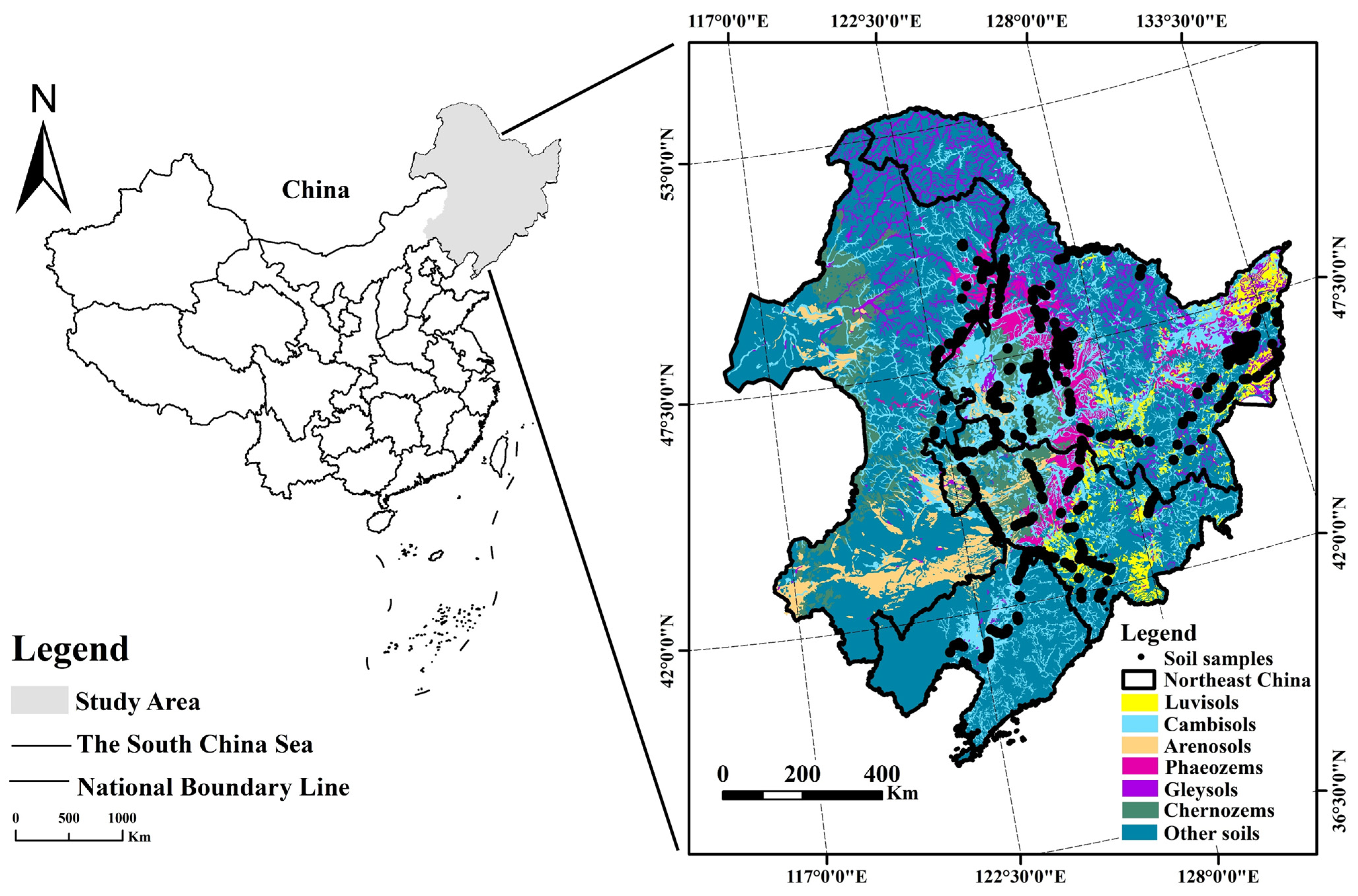
The study area was the northeastern region of China, which includes Heilongjiang, Jilin, Liaoning, and the four eastern leagues of Inner Mongolia (115.52°E–135.09°E and 38.72°N–53.56°N). The area is approximately 1,030,000 km2 and has a temperate continental monsoon climate. Annual precipitation ranges from 300 to 950 mm, with an average of 506 mm. It decreases from southeast to northwest. The landforms include plains, plateaus, hills, and mountains, and the soil types are dominated by Phaeozems, Chernozems, Cambisols, dark brown loams, Arenosols, Luvisols, Gleysols, and other soil types.
Phaeozems have a thick soil layer with a good soil structure, loose soil texture, good drainage, high water-holding capacity, and high organic matter content. Chernozems have a deep humus layer, and the lower and middle parts are calcium carbonate deposits with high potential fertility. Gleysols are composed of a peat layer (T-layer) and a submerged layer (G-layer). The former is rich in organic matter, and the latter has an organic matter content of 11.0%. The parent material of Luvisols is mainly composed of Quaternary river and lake sediments, with a barren layer of a white slurry, which has a sticky and heavy texture and low water permeability. Arenosols have a lower organic matter content than Phaeozems and Chernozems, a loose soil structure, and a fine sandy texture. They have low water and fertilizer retention capacity and are susceptible to wind and water erosion. Cambisols are typically located in low-lying terrains, often interspersed among other soil types. They have high porosity, high organic matter content, and good aeration and are susceptible to wind erosion, resulting in low topsoil quality.
2.2. Soil Sample Collection and Processing
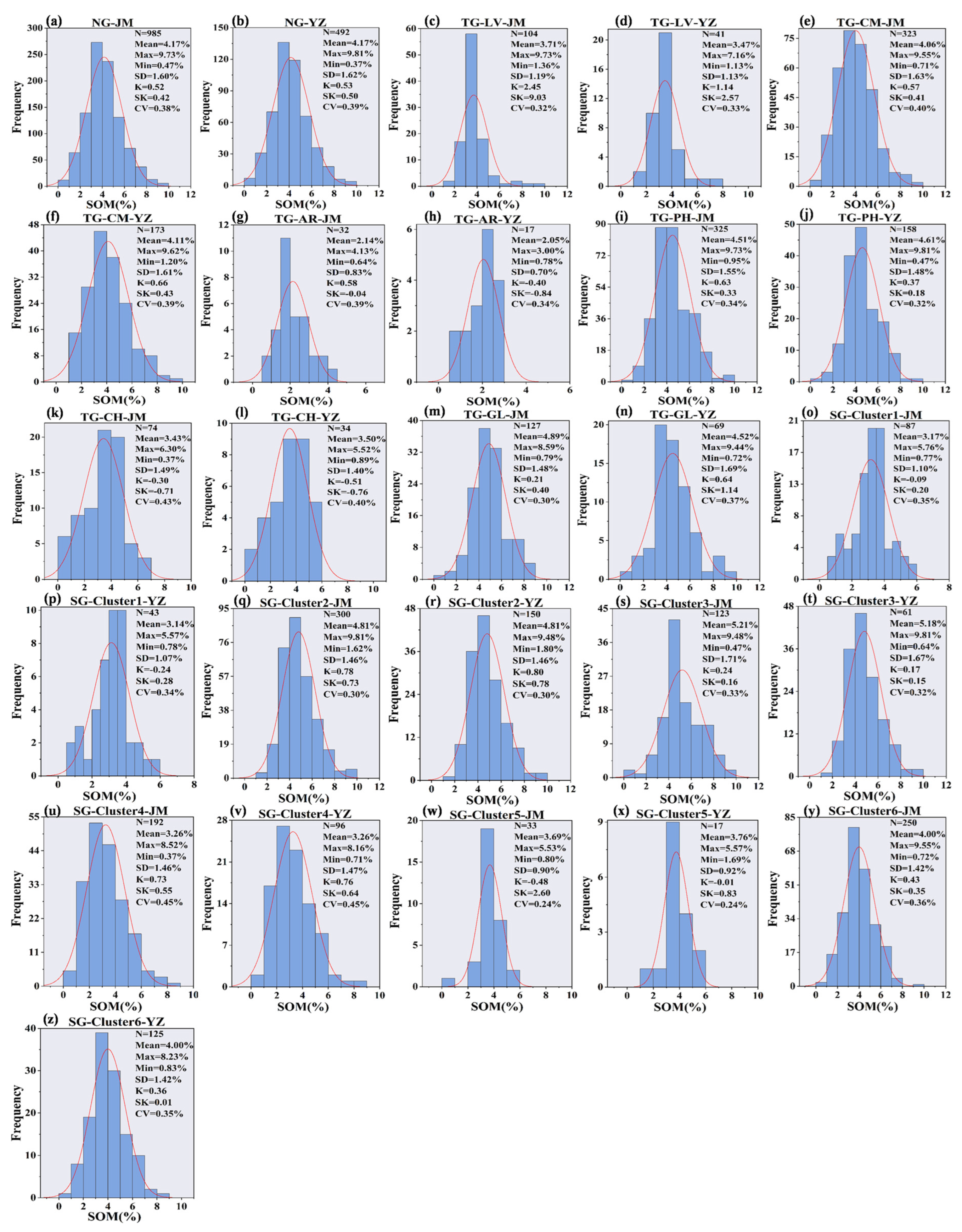
We collected 1477 topsoil samples from the 0–20 cm layer in the northeast (
Figure 1), including Luvisol, Cambisol, Arenosol, Phaeozem, Chernozem, and Gleysol samples (
Table 1). The soil samples were air-dried and milled to obtain a particle size smaller than 2 mm. Each soil sample was divided into two parts, one for spectroscopic measurements and the other for the analysis of the SOM content (%). We obtained reflectance spectra of the soil samples for subsequent analyses. The organic carbon content was determined by the high-temperature exothermic potassium dichromate oxidative capacity method [
28]. The resulting value was multiplied by 1.724 to convert it to SOM content [
29].
2.3. Soil Spectrometry
A FieldSpec@3 portable spectrometer (Analytical Spectral Devices (ASD), Boulder, CO, USA) was used in the laboratory to obtain the spectra of the soil samples. The soil samples were scraped with a straightedge, and the collected material was placed in dishes with a diameter of 12 cm and a depth of 1.8 cm. A 50 W halogen lamp 100 cm from the soil sample surface was used as the light source, with a zenith angle of 30°. The light was parallel to the soil sample surface to minimize the shadow effect caused by soil roughness. A sensor probe with an 8° field of view was placed 15 cm from the surface and perpendicular to the soil sample. The impact of the dark current was eliminated before testing, and calibration was performed with a whiteboard. Ten spectral curves were obtained for each soil sample, and the arithmetic mean was calculated and utilized for subsequent analysis.
2.4. Spectral Data Preprocessing
Most of the noise is concentrated in the ranges of 350–430 nm and 2400–2500 nm; therefore, we selected 430–2400 nm as the wavelength range [
30]. The following processing methods were adopted to eliminate spectral noise and redundant information and enhance the quality of the spectral data.
- (1)
Savitzky–Golay convolutional smoothing (S-G)
Smoothing is a standard preprocessing method used in spectral analysis [
31]. The spectral data were smoothed using S-G and a 9 × 9 window to reduce noise interference [
32,
33]. The spectral library function in ENVI version 5.3 was used to resample the spectral reflectance data to 10 nm [
34]. The result was the initial reflectance (RR) data.
- (2)
Continuum removal (CR)
CR is used to normalize the reflectance spectra. It removes baseline drift and background noise from the spectrum and improves spectral accuracy and stability [
35]. Each peak has a value of 1 after CR, and the non-peak values are less than 1, resulting in reflectance values in the range of 0–1. CR enables the comparison of reflectance values across various spectral bands. This allowed us to highlight the absorption and reflection characteristics of different soils, enhancing the variability of different soils and facilitating the extraction of features and classification analyses.
- (3)
Spectral characteristic parameters (SCPs)
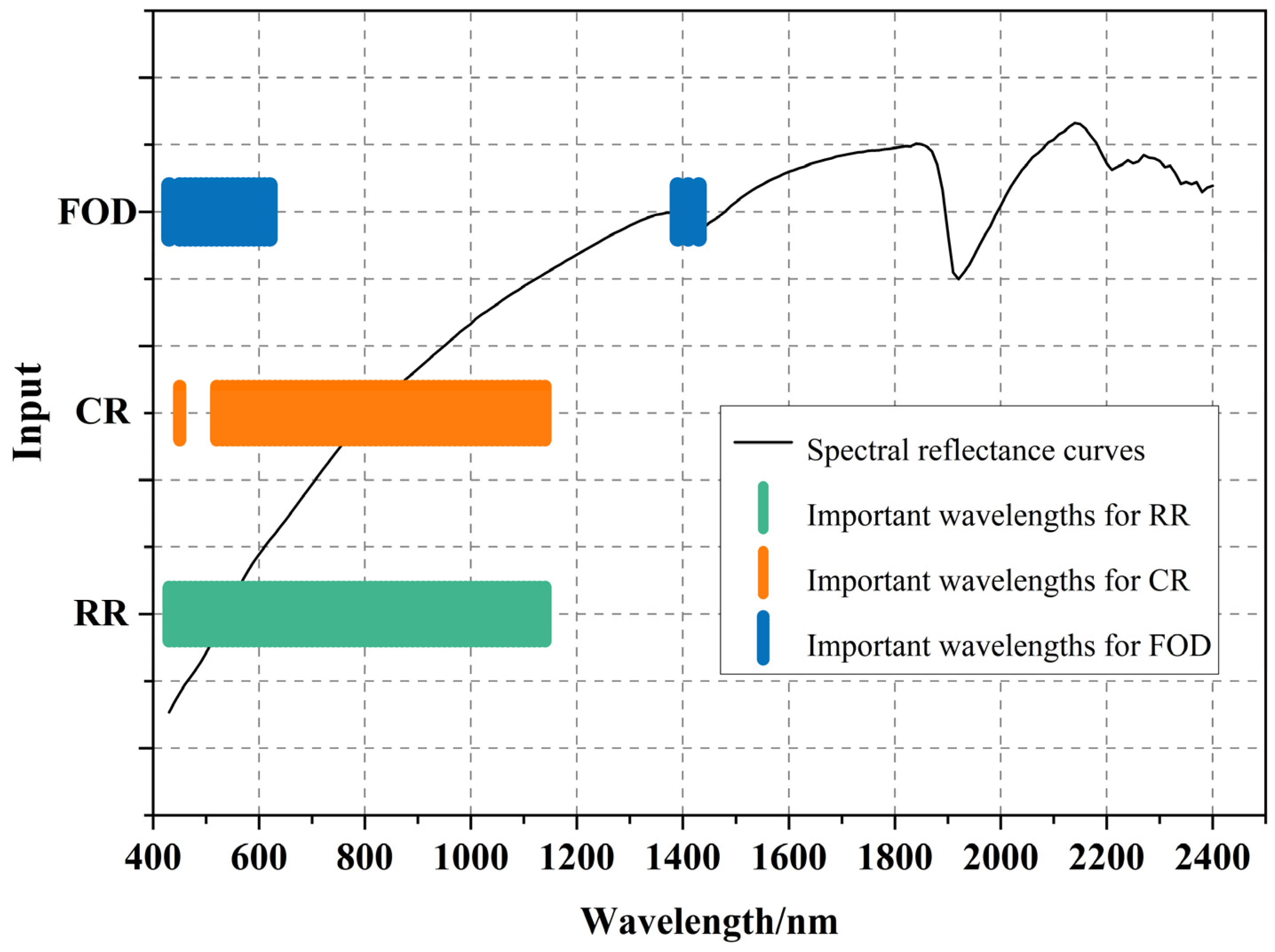
The extraction of the SCPs was based on the shape of the CR spectral curve to obtain accurate parameters. Five key absorption valleys (V
1–V
5) were extracted, and the SOM content was predicted by assessing the characteristics of the first two absorption valleys (V
1 and V
2). The SOM content affects V
1 and V
2, whereas the soil moisture content influences V
3, V
4, and V
5. Sixteen SCPs were selected based on the spectral characteristics of the soil samples (
Figure 2): the positions of the first and second absorption valleys, L
1, L
2; the absorption depths, DP
L1, DP
L2; the absorption valley areas, A
1, A
2, A
1 + A
2; the valley widths, W
1, W
2; the symmetry of the first two valleys, D
1, D
2; and the slopes between the bands of 430–510, 510–580, 580–610, 610–1120, and 510–610 nm, K
1, K
2, K
3, K
4, and K
5. These extracted spectral features were used for spectral classification and as independent variables to predict the SOM content, providing a powerful tool for soil science research. The calculation process is as follows:
where
denotes the envelope value of the
mth absorption valley position,
is the wavelength position,
is the wavelength corresponding to the left end of the
mth absorption valley,
is the wavelength corresponding to the right end of the
mth absorption valley, and
is the area of the right half of the
mth absorption valley.
- (4)
Fractional-order differentiation (FOD)
FOD is a generalization of the differential operation that extends the differential order to any non-integer order. FOD is particularly effective in amplifying subtle differences between spectral curves with nonlinear features compared to integer-order differentiation [
15]. The Grünwald–Letnikov (G-L) FOD method was used to perform differentiation of the smoothed spectral reflectance data from the zeroth to the second order (with an interval of 0.05).
where
d is the differential function,
v is the order,
h is the step size, and
a and
b are the upper and lower limits of the differential, respectively. The gamma function is defined as follows:
In this study,
h is 1, and the differential expression for the fractional differentiation of a unitary signal is defined as follows:
where
v ranges from 0 to 2 in increments of 0.05;
v = 0 denotes the initial reflectance (RR); and Equation (8) is the same as the common first-order and second-order derivative equations when
v = 1 or 2, respectively.
2.5. Grouping Approach
2.5.1. No Groups
The soil samples are not categorized in the NG approach, and the spatial differences between soil classes are ignored.
2.5.2. Traditional Grouping
TG refers to the soil classification of the second national soil census [
36]. The soil samples were classified into six classes using the macro classes. The SOM content of a subset of each soil class was predicted to capture the variability between different soil classes and improve the accuracy and precision of the prediction. The subsets’ prediction results were integrated to evaluate the overall prediction performance.
2.5.3. Spectral Grouping
SG clusters soil spectral data using K-means clustering to predict the SOM content. K-means clustering is a commonly used algorithm that classifies data by dividing the samples into a predetermined number of clusters so that each sample is associated with the nearest cluster center [
37]. We divided the soil spectral data into six classes (Clusters 1–6) and determined the optimal number of clusters based on the minimum Euclidean distance and maximum separability. After determining the optimal number of clusters, individual predictions were made for each cluster, and the results of each cluster model were integrated to evaluate the overall prediction performance.
2.6. Models
2.6.1. Random Forest (RF)
RF is an ensemble machine learning algorithm that enhances model generalization and diversity through two stochastic processes [
38]. First, bootstrap sampling is employed, where each tree uses sampling with replacement to reduce the risk of overfitting and improve model stability. Second, at each split in the decision tree, a portion of the spectral features are randomly selected as candidate features to avoid over-reliance on a single feature and improve the model’s generalization ability. In this study, the optimal number of regression trees (
ntree) and splitting nodes (
mtry) were determined by evaluating the out-of-bag error to obtain the optimal RF prediction model. The
was 500, and
was 1/3 of the number of inputs [
39]. R software (version 4.2.3) and the RF package were used to implement the RF model.
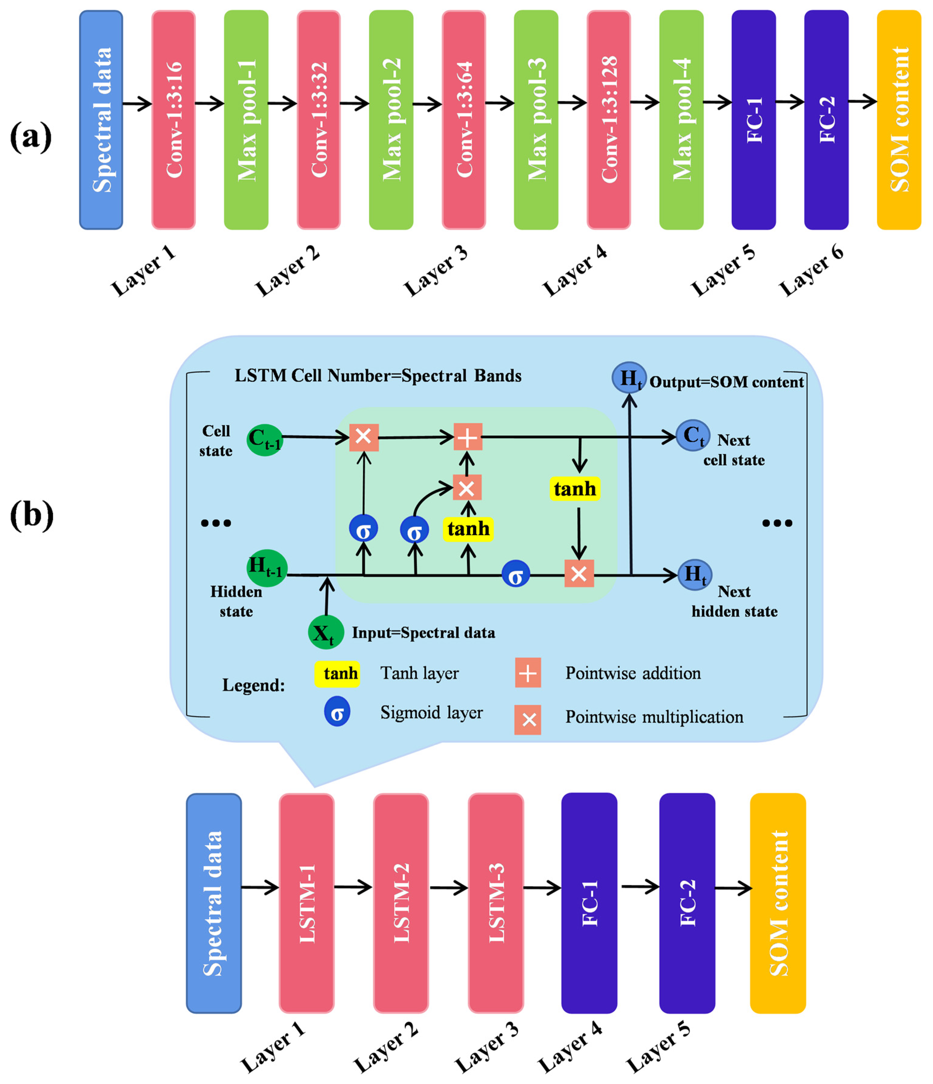
2.6.2. Convolutional Neural Network (CNN)
A CNN is a neural network model. CNNs have been used to analyze spectral data. High-level spectral features are extracted by convolutional layers, which are then passed to fully connected layers for the final prediction. Unlike manual selection of the convolution kernel, a CNN learns the convolution kernel automatically through a backpropagation algorithm. This strategy is more suitable for spectral data features. CNNs can capture the correlation between different bands in hyperspectral data through the convolution layer, enabling a better understanding of the spatial structure and features in the data. A Max-Pooling operation is applied after each convolutional layer to reduce the feature dimensionality, retain salient features, and reduce the number of parameters in subsequent convolutional layers [
40]. The ReLU activation function was used in this study to reduce the computational complexity, redundancy between parameters, and risk of overfitting. Since the soil spectral reflectance data have only one spectral dimension, a one-dimensional CNN model was chosen for predicting the SOM content. The model structure is shown in
Figure 3a. The hyperparameter settings for the model are detailed in
Table 2, comprising an input layer, four convolutional layers, four pooling layers, two fully connected layers, and one output layer.
2.6.3. Long Short-Term Memory (LSTM)
An LSTM model is a type of recurrent neural network (RNN) that is widely used for modeling and prediction using sequential data [
41]. Unlike traditional RNNs, LSTMs solve the long-term dependency and gradient vanishing problems by using a gating mechanism. In this study, the LSTM model was employed for predicting SOM content. LSTMs can handle sequential data, such as spectral data, efficiently. A critical component in the LSTM model is the memory cell, which stores and updates information. The memory cell consists of forgetting, input, and output gates, which determine the importance of the spectral data, adjust the memory state, and generate new candidate values through a sigmoid activation function. The Tanh activation function was used for the final prediction of the SOM content. The LSTM model possesses excellent performance for processing sequential data, enabling it to capture the long-term dependencies within the dataset. The structure of the model is shown in
Figure 3b. The hyperparameter settings for the model are detailed in
Table 3.
2.7. Model Evaluation
The soil samples were divided into modeling and validation sets using a ratio of 2:1. Subsets of soil types were also divided using the same 2:1 ratio. The RF, CNN, and LSTM models were used to predict the SOM content. Model accuracy was compared using the coefficient of determination (R2), root mean squared error (RMSE), ratio of performance to interquartile distance (RPIQ), and residual prediction deviation (RPD).
where
m is the number of samples,
is the measured SOM content at the
mth sample point,
is the predicted SOM content at the
mth sample point, and
is the average SOM content at all sample points. The larger the
R2,
RPIQ, and
RPD and the smaller the
RMSE, the higher the model’s predictive ability.
4. Discussion
This study differs from others predicting SOM content by employing an integrated approach. Unlike studies focusing on a single factor (e.g., grouping method, number of inputs, or prediction model), we considered all three critical elements to address the complexity of SOM content prediction for large-scale farmland. Due to the heterogeneity of SOM, an optimal combination of the grouping method, input volume, and prediction model is required for predicting the SOM content in large regions due to the SOM heterogeneity. The LSTM model precisely captured the relationship between the SOM content and the spectral features; thus, it was the most suitable prediction algorithm for the SOM content in this study. We identified significant differences in the spectral features of different soil types. Therefore, we used SG combined with the K-means method to cluster the spectral features of different soil classes. This approach strengthened our study by providing a more accurate classification of different soil samples. We provide here an in-depth discussion on the impact of several key factors on SOM content prediction, practical recommendations for selecting deep learning models and hyperspectral data, and the limitations of this study.
4.1. Impact of Deep Learning on the Performance of SOM Content Prediction Models
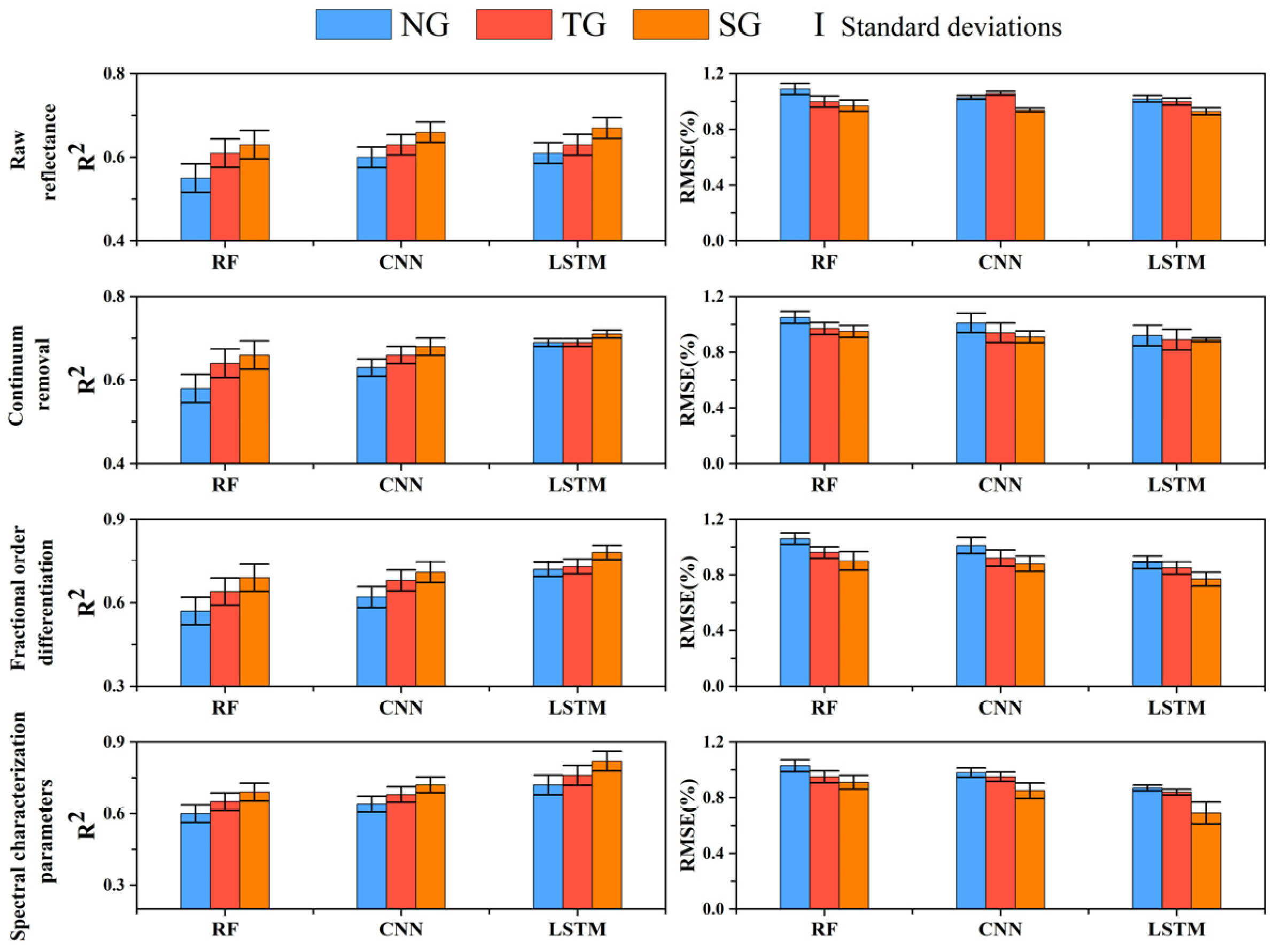
The comprehensive comparison of three different algorithms indicates that LSTM and CNN models outperform RF models in predicting SOM content. Our approach demonstrates flexibility in adapting to hyperspectral data and provides high performance (
Figure 9). The LSTM model, as a type of recurrent neural network with memory functionality, swiftly captures intricate nonlinear relationships and exhibits robust modeling capabilities for continuous data. Consequently, as depicted in
Figure 9, in this study, the accuracy of LSTM in predicting SOM content surpasses the other two models, with an R
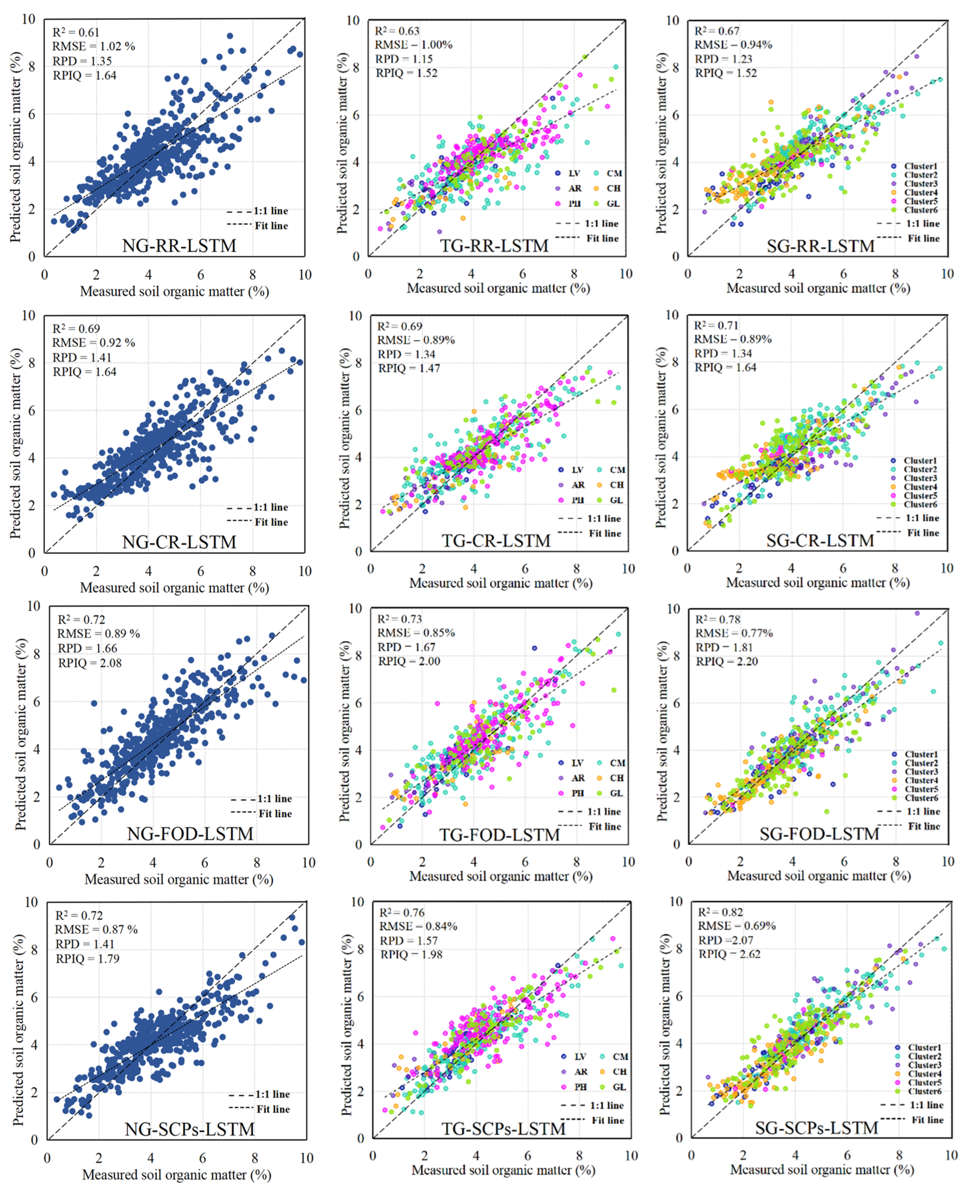
2 of approximately 0.82, an RMSE of about 0.69%, a PRIQ of around 2.62, and an RPD of approximately 2.07. In comparison to RF, CNN and LSTM are more adept at considering sequential features, thereby enhancing model robustness and reducing errors. For preprocessing hyperspectral data, we observed that spectral feature parameters significantly improve deep learning models. Machine learning algorithms, such as RF, coupled with 1.05-order FOD spectral preprocessing, can extract spectral features and achieve performance levels similar to deep learning models. Overall, the LSTM model performs the best, followed by CNN, and RF ranks last. LSTM is suitable for spectral data with limited wavelength inputs, while CNN is effective for features such as hyperspectral reflectance.
In addition, we observed that the performance of the hyperspectral reflectance data did not significantly improve the performance of the LSTM and CNN models. These two highly nonlinear deep learning models already have strong feature learning capabilities and can fit the relationship between the spectral features and the SOM content without much preprocessing. Meanwhile, the performance of the RF model was significantly improved by spectral preprocessing, especially when the FOD was used as the input.
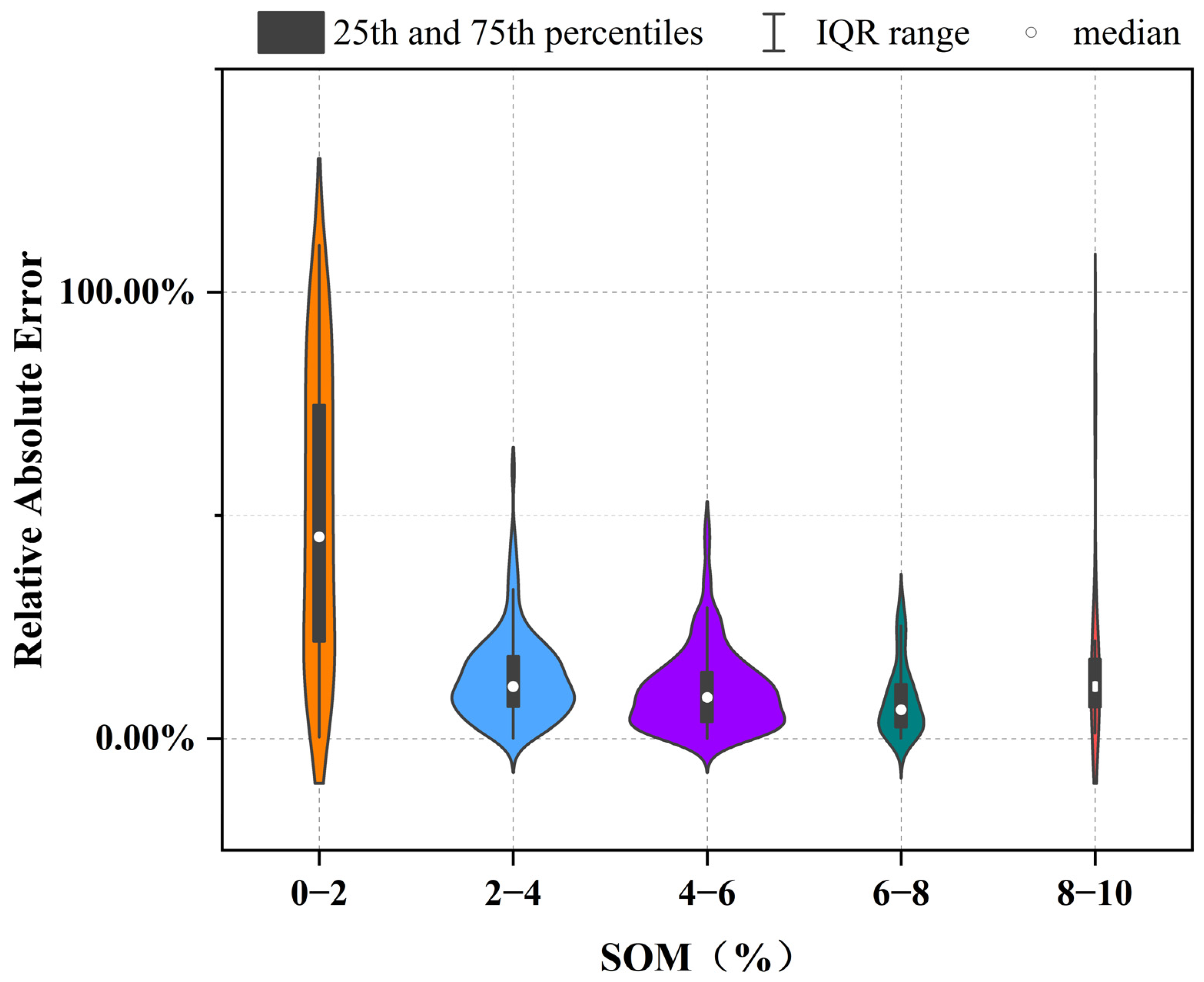
The LSTM model’s uncertainty was evaluated by calculating the relative absolute error (RAE) and dividing the SOM content into five intervals (
Figure 10). The model’s RAE was significantly correlated with the SOM content. The LSTM model had high prediction errors at low (0–2%) and high (8–10%) SOM contents, with lower prediction errors observed at intermediate contents (2–8%).
4.2. Comparison of Grouping Methods and Inputs
Guerrero et al. [
42] found that local regression was superior to global regression. In this study, three groupings (NG, TG, and SG) and four input variables (RR, CR, FOD, and SCPs) were selected. Consistent with previous studies [
43], local regression resulted in a higher accuracy in SOM prediction compared to the NG method, confirming the significance of soil grouping for SOM prediction in large areas.
The rationales of the different methods resulted in differences in the number of variables and locations. The results showed that variable selection helped to reduce model complexity by eliminating redundant variables and retaining only those significantly correlated with the SOM content. The methods based on the four inputs had higher accuracy than the model using all bands. The SOM prediction performance is related to the spectral preprocessing method [
9,
44]. It has been shown that mathematical methods for resampling the spectral curves and enhancing the linearity of the spectral features improved prediction accuracy. For example, spectral reflectance curves are subjected to derivative operations using mathematical transformations, such as first-order differentiation, logarithmic, and inverse transformations [
45], or CR to amplify the local absorption features of the spectral curves [
46]. However, these methods have limitations, i.e., mathematical transformations may increase the noise level [
47]. The number of bands remains the same after mathematical transformations; therefore, dimensionality reduction techniques such as principal component analysis (PCA) or competitive adaptive reweighting (CARS) can be considered [
48,
49]. Limiting the spectral range to 400–1200 nm resulted in higher correlations between the spectral features and the SOM content [
50].
The TG resulted in significantly higher prediction accuracy of the SOM content than NG (
Figure 8); i.e., the R
2 was 0.21 higher, the RMSE was 25% lower, the RPIQ was 0.67 higher, and the RPD was 0.45 higher. The reason for this is that the soil samples were obtained from multiple soil types. Due to differences in the soil parent material and soil structure, the spectral characteristics differed for different soil types, affecting the prediction accuracy. The spectral differences among the soil classes were lower after TG. For instance, the first two absorption valleys of different soil classes were dissimilar after CR. The first two absorption valleys of the Phaeozems were profound, with the second one being larger than the first one. In contrast, the first absorption valley of the Arenosols was symmetric, and the second one was smaller. Thus, SG improved the accuracy of SOM prediction.
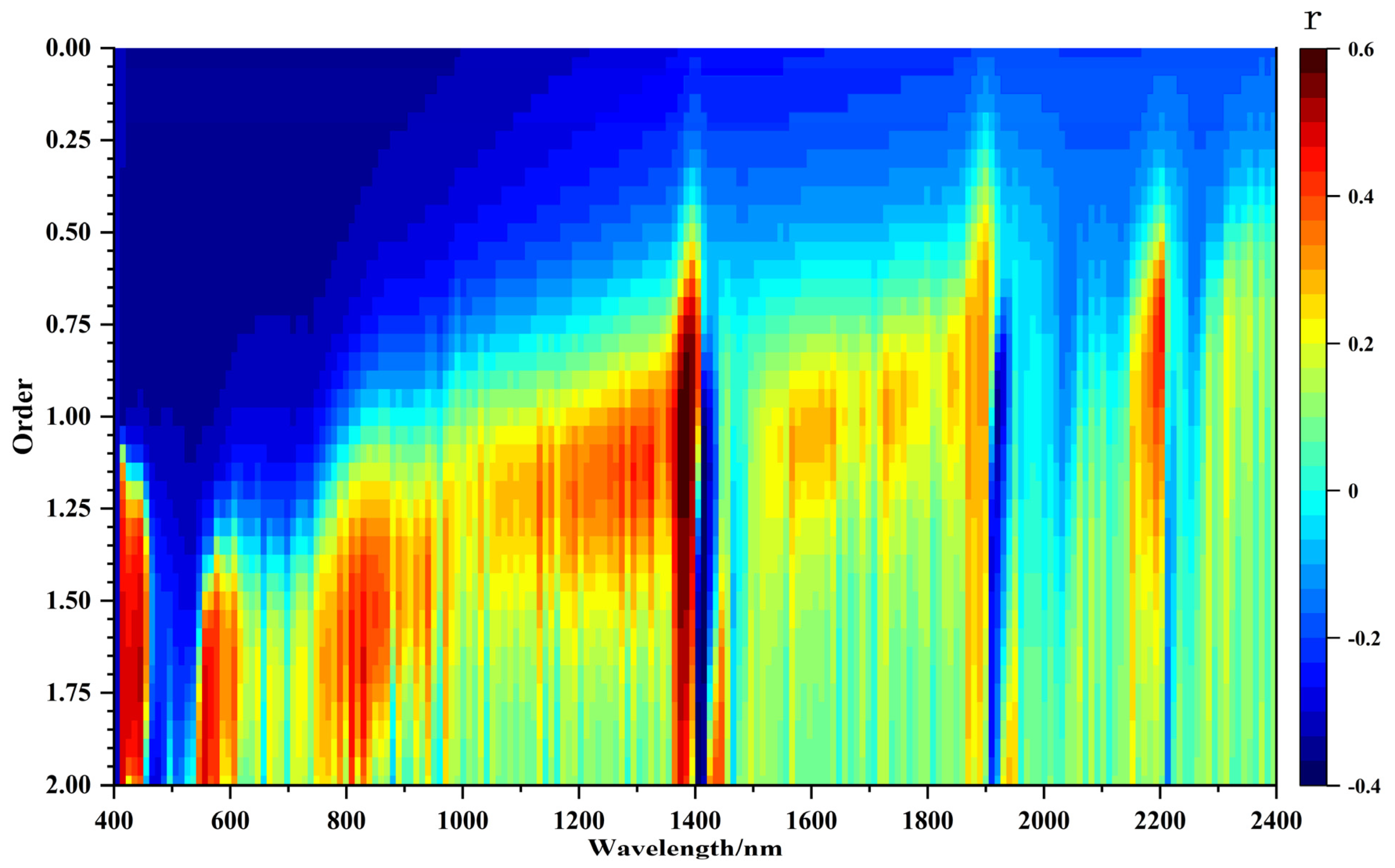
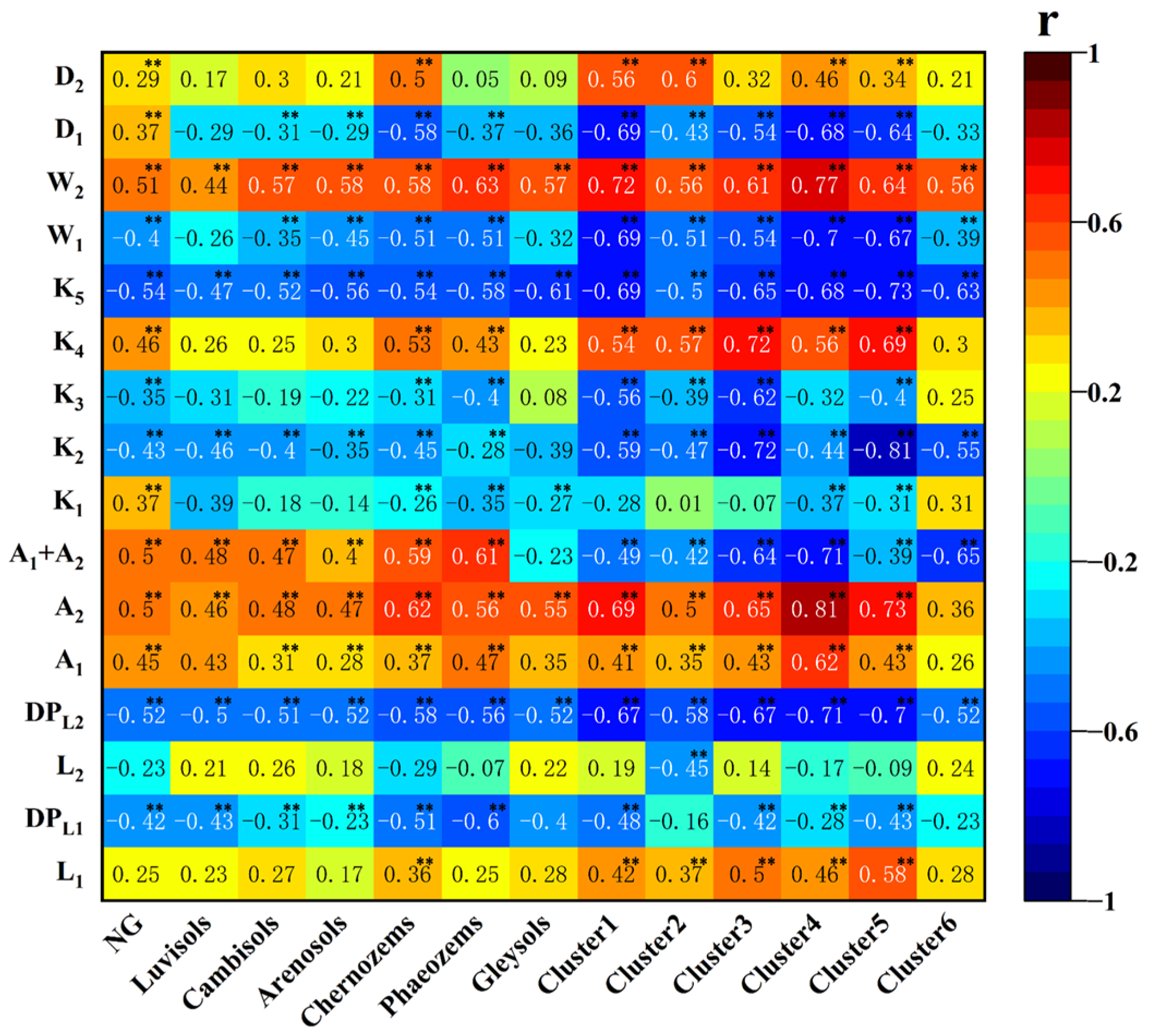
We found that the model with SG and taking the SCPs as input variables performed the best and provided the highest accuracy. SCPs are indicators of soil chemical and physicochemical properties and are highly informative for predicting the SOM content. They were generally highly correlated with the SOM content (
Figure 11). DP
L2, A
2, A
1 + A
2, K
5, and W
2 had the highest correlations. The correlation was higher between SCPs and the SOM content of Phaeozems when TG was used as a grouping method, with a W
2 of 0.63. Only DP
L2 exceeded 0.5 for Luvisols. For SG, Cluster 4 had the highest correlation, with an A
2 of 0.81. Except for Clusters 2 and 6, all other clusters had correlation coefficients exceeding 0.7. These significant correlations indicate that the spectral features were extracted more efficiently using SG to improve the model’s generalization ability. FOD improved the SOM prediction accuracy by capturing the features of the first two absorption valleys of the spectral curves after CR. CR and FOD performed comparably as input variables in terms of prediction accuracy.
4.3. Research Limitations
The results of this study showed that the combination of SG, SCPs, and the deep learning LSTM algorithm was the most effective method for predicting SOM content in Northeast China. Although deep learning has high accuracy, it is challenging to determine the optimal parameters quickly due to the complex network structure [
51,
52]. Therefore, more efficient parameter optimization methods, such as stochastic search or Bayesian optimization, must be considered to optimize model performance. In addition, dropout layers or other activation functions can be incorporated to improve model performance [
53]. The training data for the model were soil data from the northeast region of China. However, the model’s generalization performance should be validated in other regions, as soil properties and environmental conditions in different regions may impact its applicability. Other factors, such as soil moisture, texture, and soil parent material, must be considered when applying the model to other regions. Although several methods and algorithms were used in this study for SOM content prediction, the results have uncertainty. Therefore, the confidence interval or error range should be considered in practical applications. This paper considered only spectral features in the visible, NIR, and shortwave infrared bands. The mid-infrared and thermal infrared bands could be assessed in future studies, expanding the spectral measurement range. In addition, future research could consider optimizing inputs, selecting different algorithms, and considering more uncertainties for SOM prediction.
5. Conclusions
This study evaluated the potential of combining different algorithms, grouping methods, and inputs for SOM prediction using hyperspectral reflectance data from 1477 surface soil samples in Northeastern China. The algorithms included RF, CNN, and LSTM models, with the grouping methods comprising NG, TG, and SG and the inputs including RR, CR, FOD, and SCPs. The study revealed that the LSTM model with SG and SCP inputs obtained the highest prediction accuracy. The LSTM model extracted the deep relationships between the spectral data and the SOM content. SG reduced the variability in the spectral features among different soil classes, and the SCPs reflected the absorption features of the spectral curves so that different soil samples could be distinguished accurately. This combination provided the most accurate results for soil property assessment. The ranking of the models for SOM content prediction was LSTM > CNN > RF, and the ranking of the grouping approach was SG > TG > NG. When SCPs were used as inputs, the RMSE was 0.24%, 0.20%, and 0.08% lower, and the R2 was 0.15, 0.11, and 0.04 higher, respectively, than for the other models. This study also identified the optimum SCPs (DPL2, A2, A1 + A2, and W2) for SOM content prediction. However, the predictive ability of the LSTM model varied for different SOM content ranges. Small errors were observed at intermediate SOM contents (2–8%), whereas relatively large errors occurred at low (0–2%) and high (8–10%) contents. This discrepancy was attributed to the model’s ability to learn the data distribution for different content ranges. Further research is required to optimize the model’s performance. The deep learning model mined the relationship between spectral features and SOM content using different grouping methods and inputs, achieving high-precision SOM content prediction in a large area. The study results strongly support the improvement in large-scale SOM content prediction accuracy and reduction in spatial heterogeneity in large regions, and offer scientific methods and foundations for the future prediction of SOM content snapshots.


 ,
, 


