
Remote Sensing Identification and Spatiotemporal Change Analysis of Cladophora with Different Morphologies

 ,
,
Abstract
1. Introduction
2. Materials
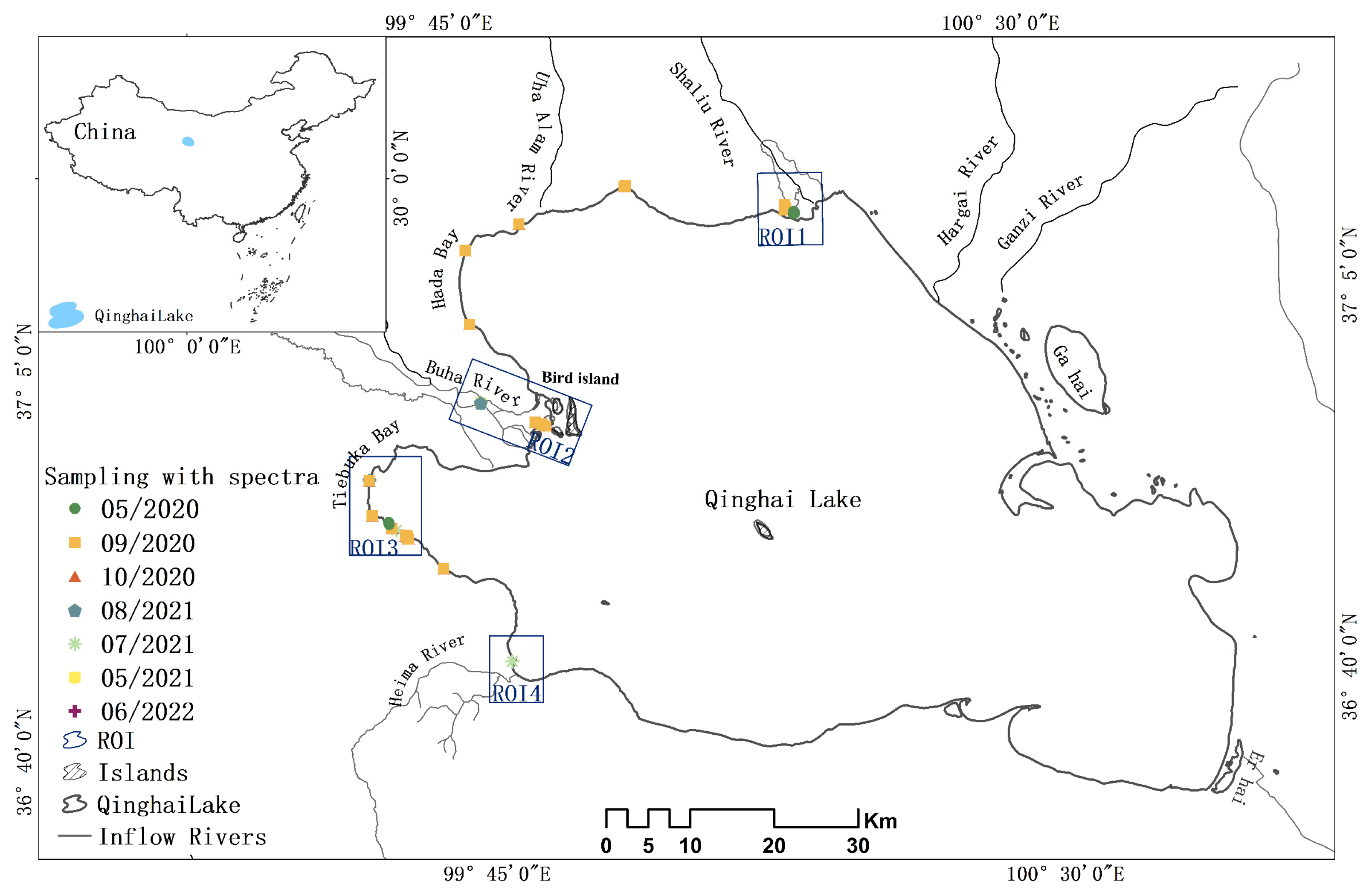
2.1. Study Area
2.2. Data Source
2.2.1. Measured Data
2.2.2. Remote Sensing Images
3. Methods
3.1. Remote Sensing Data Preprocessing
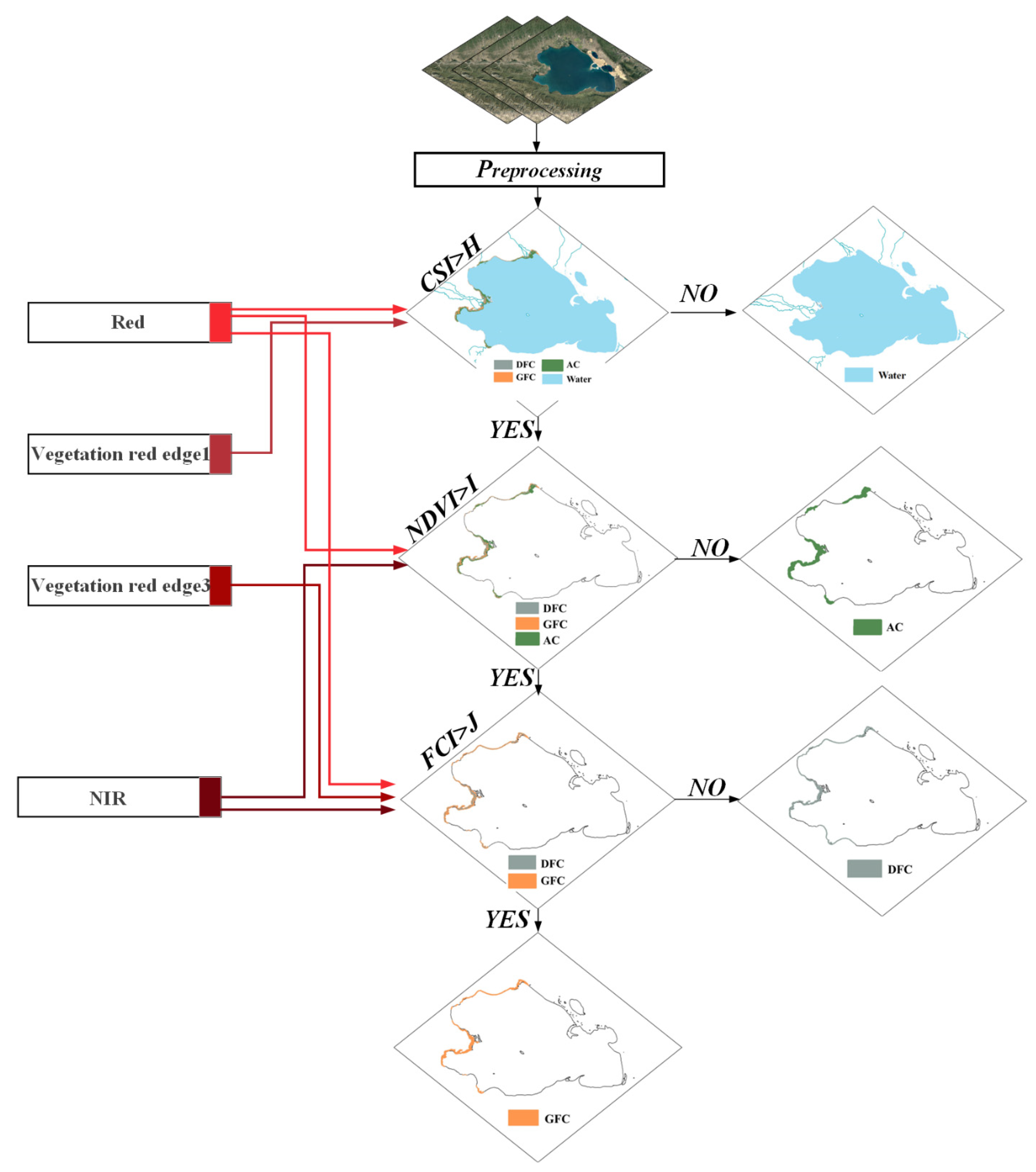
3.2. Classification Decision Tree Model for Three Cladophora Morphologies Using Sentinel-2 Data
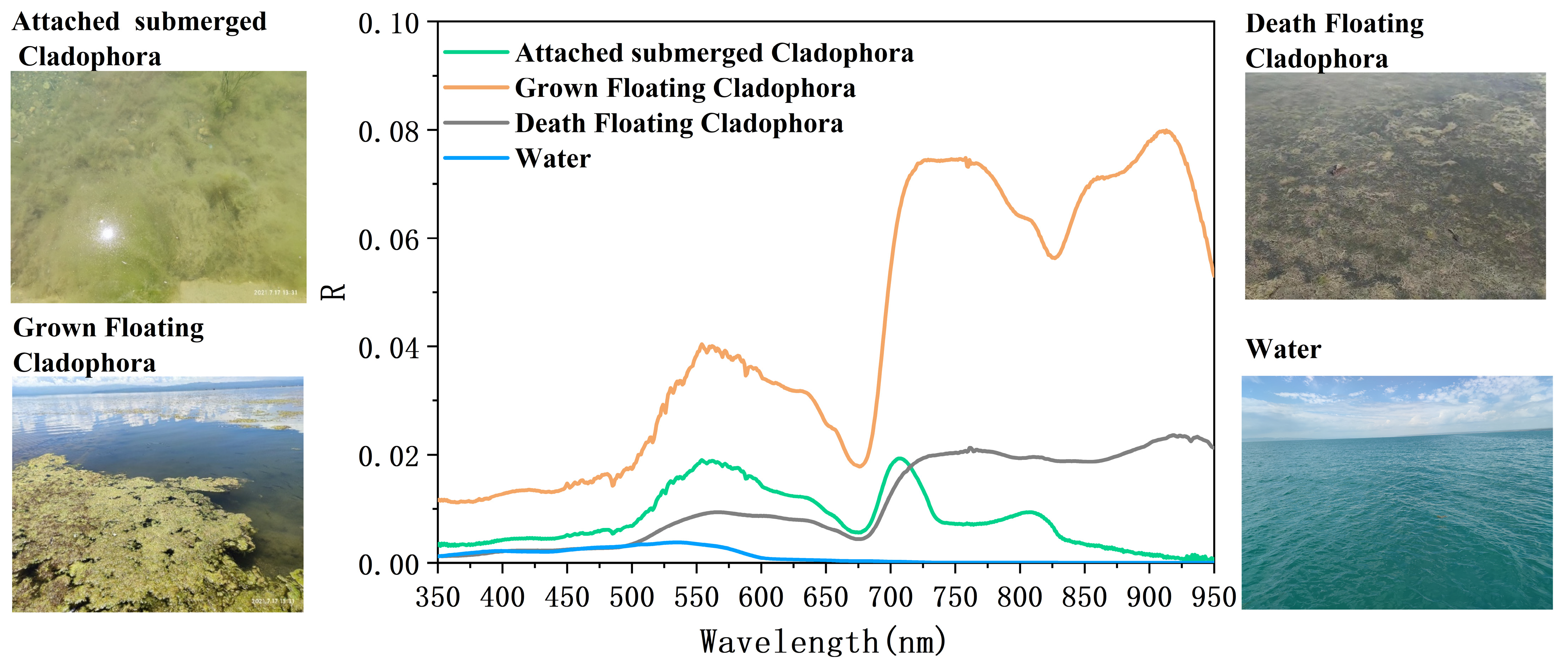
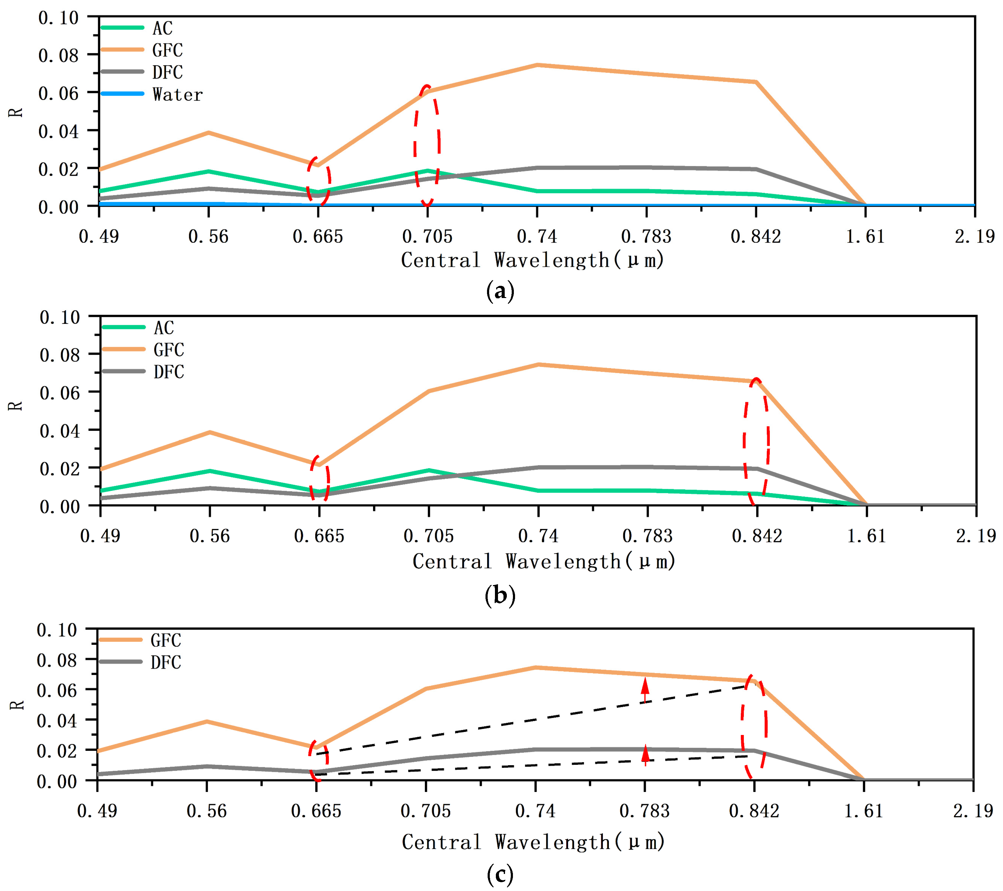
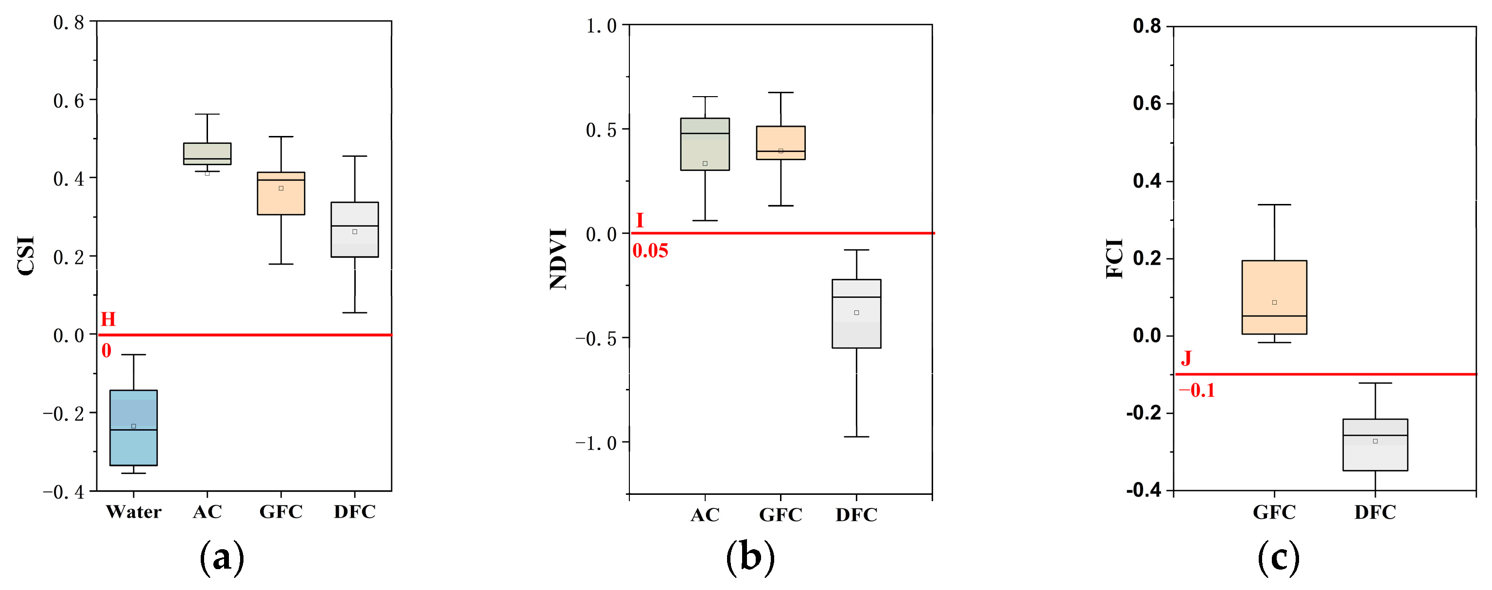
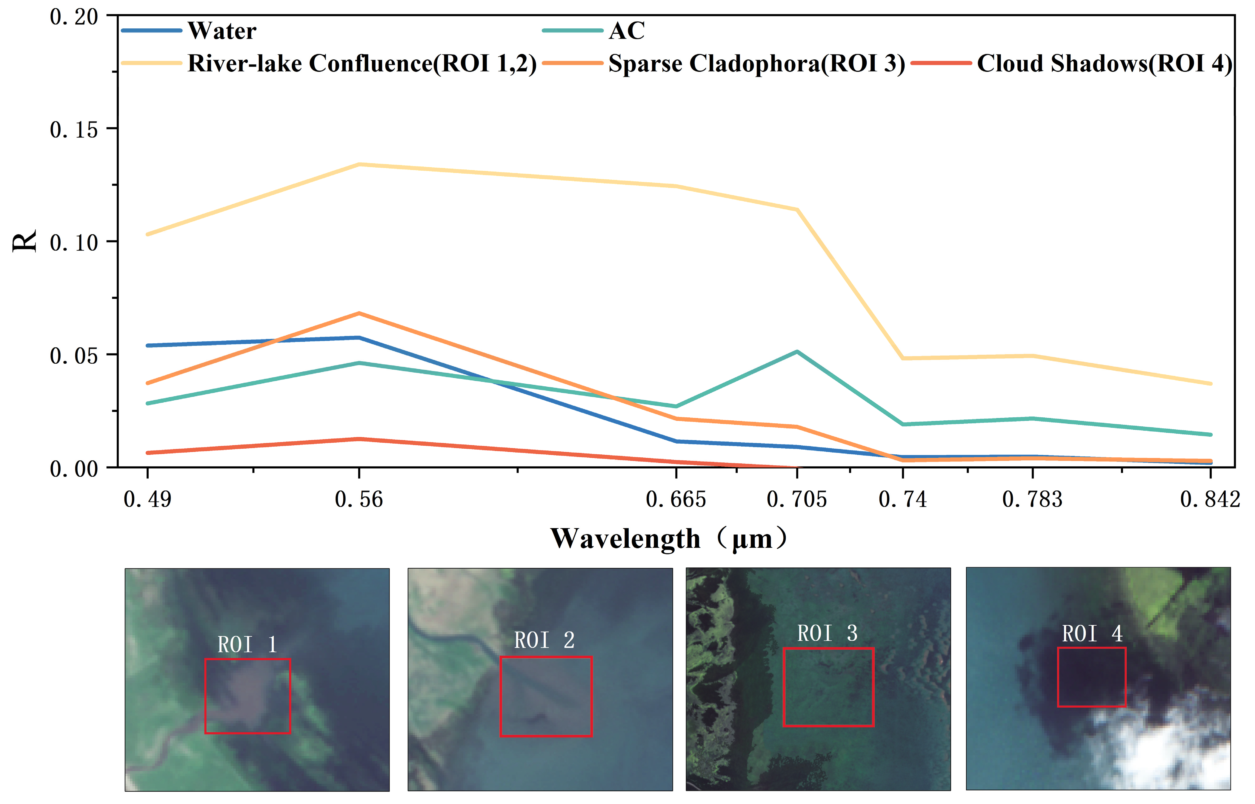
3.2.1. Spectral Characteristics and Indices Selection
3.2.2. Classification Decision Tree Model and Threshold Selection
3.3. Visual Interpretation for Two Cladophora Morphologies Using Landsat
3.4. Accuracy Assessment
4. Results
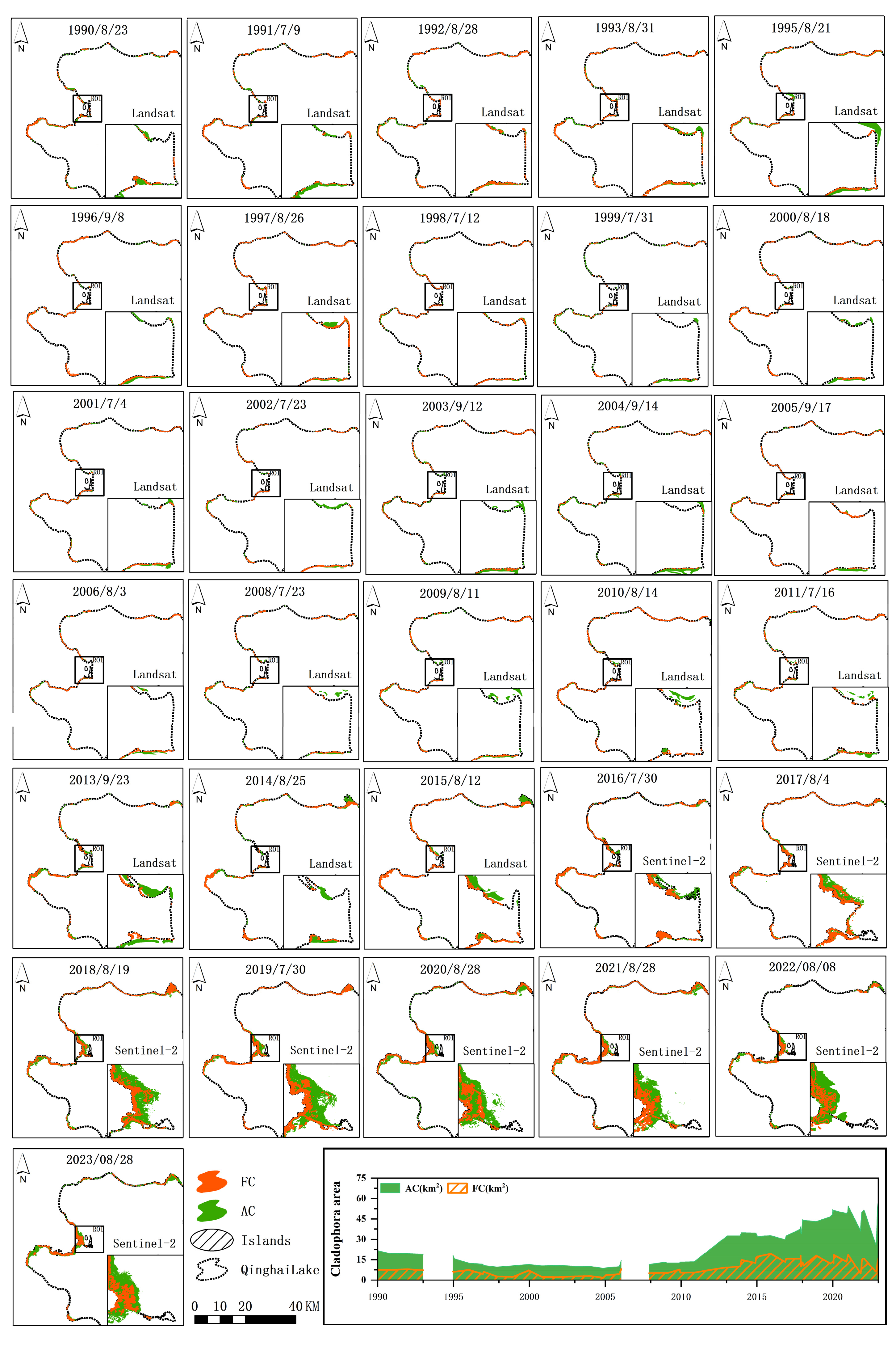
4.1. Interannual Variation Characteristics of Three Cladophora Morphologies
4.2. Interannual Spatiotemporal Characteristics of Two Morphologies Cladophora
4.3. Comparison of Cladophora Classification from Different Remote Sensing Images
4.3.1. Validating the Identification Accuracy of Cladophora Using High Resolution Images
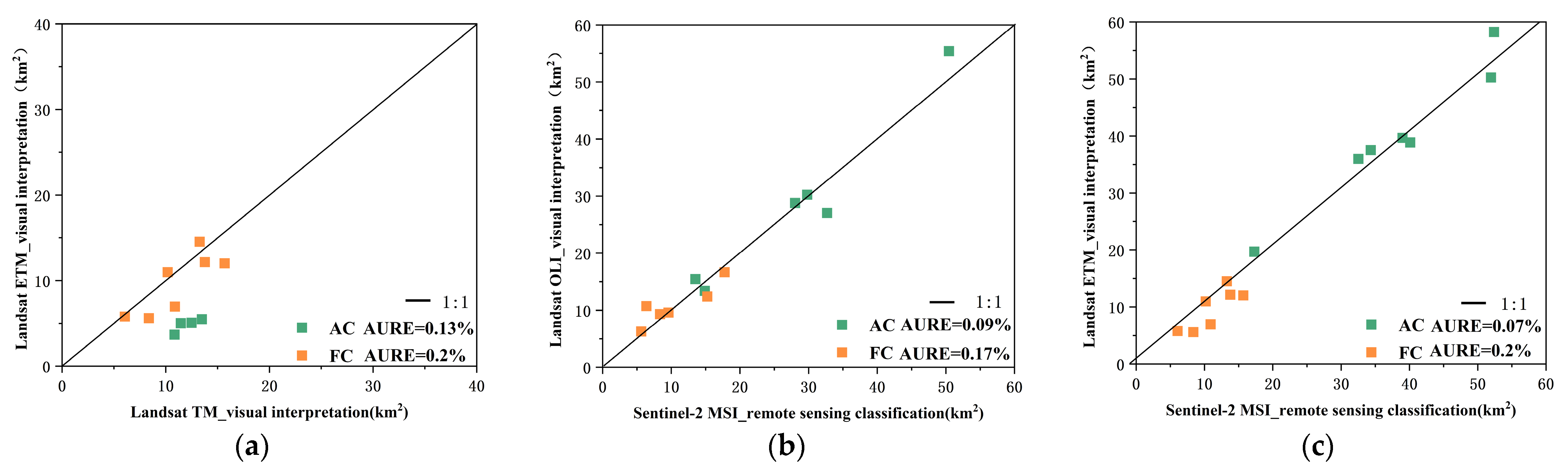
4.3.2. Cross-Validating Landsat and Sentinel-2-Based Identification of Cladophora
5. Discussion
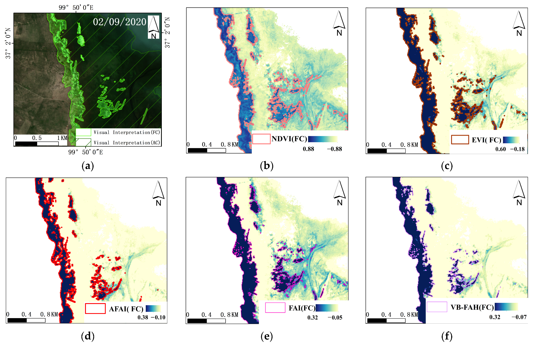
5.1. The Applicability of Classification Decision Tree Model to Other Spectral Indices
5.2. Analysis of Driving Forces Affecting Changes in Cladophora
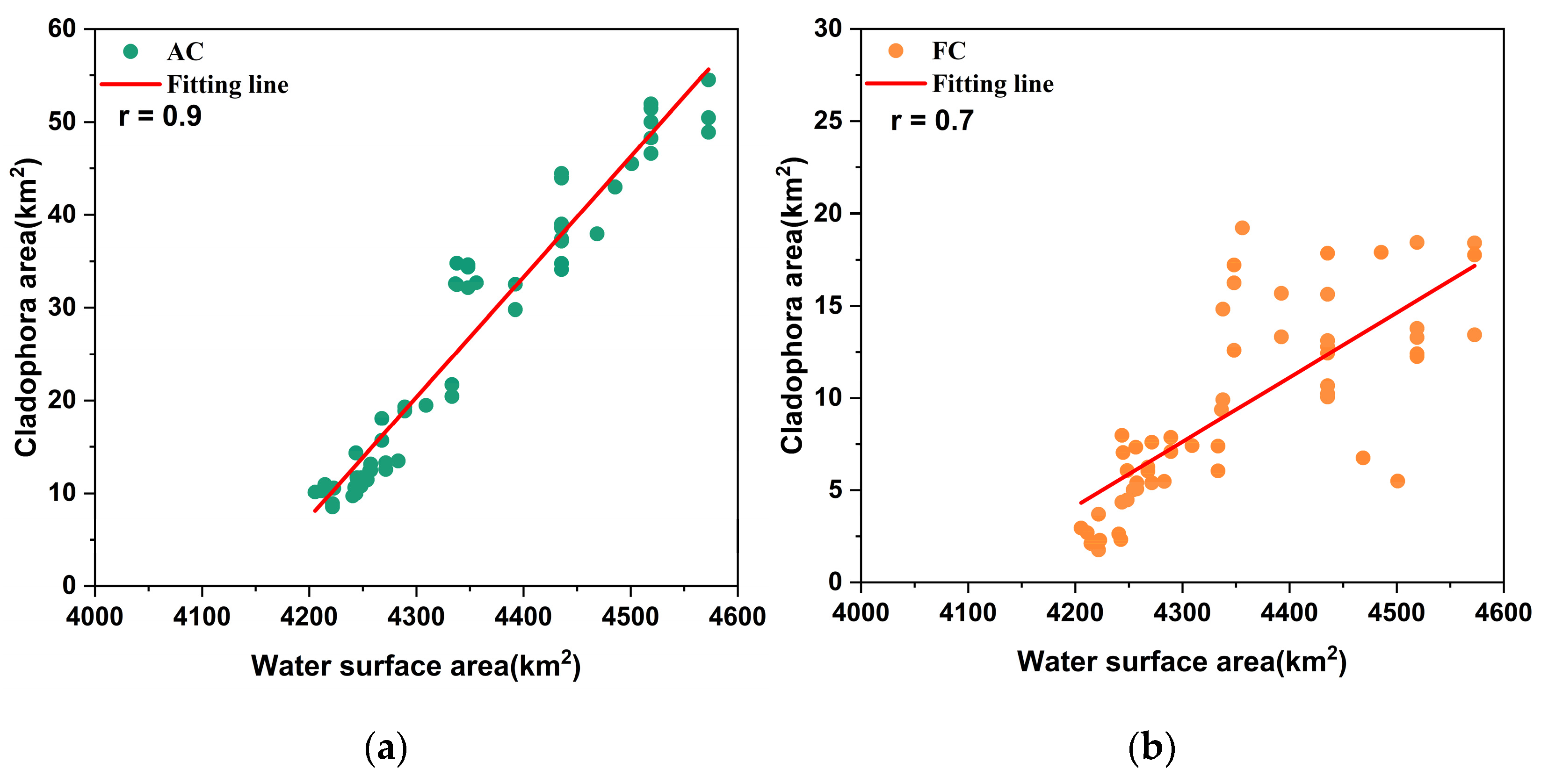
5.2.1. Water Surface Area
5.2.2. Climatic Factors
5.3. CDTM Applicability Analysis
6. Conclusions
Author Contributions
Funding
Data Availability Statement
Conflicts of Interest
References
- Gower, J.; Hu, C.; Borstad, G.; King, S. Ocean color satellites show extensive lines of floating sargassum in the gulf of Mexico. IEEE Trans. Geosci. Remote Sens. 2006, 44, 3619–3625. [Google Scholar] [CrossRef]
- Hu, C.; Lee, Z.; Ma, R.; Yu, K.; Li, D.; Shang, S. Moderate resolution imaging spectroradiometer (MODIS) observations of cyanobacteria blooms in Taihu Lake, China. J. Geophys. Res. Ocean 2010, 115, C4. [Google Scholar] [CrossRef]
- Hu, C.; Li, D.; Chen, C.; Ge, J.; Muller-Karger, F.E.; Liu, J.; Yu, F.; He, M.X. On the recurrent Ulva prolifera blooms in the Yellow Sea and East China Sea. J. Geophys. Res. Ocean 2010, 115, C5. [Google Scholar] [CrossRef]
- Wynne, T.T.; Stumpf, R.P.; Tomlinson, M.C.; Dyble, J. Characterizing a cyanobacterial bloom in western Lake Erie using satellite imagery and meteorological data. Limnol. Oceanogr. 2010, 55, 2025–2036. [Google Scholar] [CrossRef]
- Gower, J.; Young, E.; King, S. Satellite images suggest a new Sargassum source region in 2011. Remote Sens. Lett. 2013, 4, 764–773. [Google Scholar] [CrossRef]
- Shuchman, R.A.; Sayers, M.J.; Brooks, C.N. Mapping and monitoring the extent of submerged aquatic vegetation in the laurentian great lakes with multi-scale satellite remote sensing. J. Great Lakes Res. 2013, 39, 78–89. [Google Scholar] [CrossRef]
- Qi, L.; Hu, C.; Wang, M.; Shang, S.; Wilson, C. Floating Algae Blooms in the East China Sea. Geophys. Res. Lett. 2017, 44, 11501–11509. [Google Scholar] [CrossRef]
- Blondeau-Patissier, D.; Brando, V.E.; Lønborg, C.; Leahy, S.M.; Dekker, A.G. Phenology of Trichodesmium spp. blooms in the Great Barrier Reef lagoon, Australia, from the ESA-MERIS 10-year mission. PLoS ONE 2018, 13, e0208010. [Google Scholar] [CrossRef] [PubMed]
- Xing, Q.; An, D.; Zheng, X.; Wei, Z.; Wang, X.; Li, L.; Tian, L.; Chen, J. Monitoring seaweed aquaculture in the Yellow Sea with multiple sensors for managing the disaster of macroalgal blooms. Remote Sens. Environ. 2019, 231, 111279. [Google Scholar] [CrossRef]
- Qi, L.; Tsai, S.F.; Chen, Y.; Le, C.; Hu, C. In Search of Red Noctiluca scintillans Blooms in the East China Sea. Geophys. Res. Lett. 2019, 46, 5997–6004. [Google Scholar] [CrossRef]
- Zhang, B.; Li, J.; Shen, Q.; Wu, Y.; Zhang, F.; Wang, S.; Yao, Y.; Guo, L.; Yin, Z. Recent research progress on long time series and large scale optical remote sensing of inland water. Natl. Remote Sens. Bull. 2021, 25, 37–52. [Google Scholar] [CrossRef]
- Lyons, D.A.; Arvanitidis, C.; Blight, A.J.; Chatzinikolaou, E.; Guy-Haim, T.; Kotta, J.; Orav-Kotta, H.; Queirós, A.M.; Rilov, G.; Somerfield, P.J.; et al. Macroalgal blooms alter community structure and primary productivity in marine ecosystems. Glob. Chang. Biol. 2014, 20, 2712–2724. [Google Scholar] [CrossRef]
- Ministry of Science and Technology of China. Ministry of Science and Technology Releases. Annual Report on Global Ecological Environment Remote Sensing Monitoring. 2021. Available online: http://www.most.gov.cn/kjbgz/202112/t20211222_178697.html (accessed on 22 December 2021).
- Kutser, T.; Metsamaa, L.; Strömbeck, N.; Vahtmäe, E. Monitoring cyanobacterial blooms by satellite remote sensing. Estuar. Coast. Shelf Sci. 2006, 67, 303–312. [Google Scholar] [CrossRef]
- Duan, H.T.; Zhang, S.; Zhang, Y. Cyanobacteria bloom monitoring with remote sensing in Lake Taihu. J. Lake Sci. 2008, 20, 145–152. [Google Scholar] [CrossRef]
- Ma, R.; Kong, F.; Duan, H. Spatio-temporal distribution of cyanobacteria blooms based on satellite imageries in Lake Taihu, China. J. Lake Sci. 2008, 20, 687–694. [Google Scholar]
- Gower, J.; King, S.; Goncalves, P. Global monitoring of plankton blooms using MERIS MCI. Int. J. Remote Sens. 2008, 29, 6209–6216. [Google Scholar] [CrossRef]
- Duan, H.; Ma, R.; Xu, X.; Kong, F.; Zhang, S.; Kong, W.; Hao, J.; Shang, L. Two-decade reconstruction of algal blooms in China’s Lake Taihu. Environ. Sci. Technol. 2009, 43, 3522–3528. [Google Scholar] [CrossRef]
- Hu, C. A novel ocean color index to detect floating algae in the global oceans. Remote Sens. Environ. 2009, 113, 2118–2129. [Google Scholar] [CrossRef]
- Liu, S.; Yang, M.; Zhang, F.; Zhang, S. Research on early warning of dinoflagellate bloom in Caojie Reservoir base on support vector machine classification. J. Lake Sci. 2015, 27, 38–43. [Google Scholar] [CrossRef]
- Oyama, Y.; Matsushita, B.; Fukushima, T. Distinguishing surface cyanobacterial blooms and aquatic macrophytes using Landsat/TM and ETM+ shortwave infrared bands. Remote Sens. Environ. 2015, 157, 35–47. [Google Scholar] [CrossRef]
- Shen, F.; Tang, R.; Sun, X.; Liu, D. Simple methods for satellite identification of algal blooms and species using 10-year time series data from the East China Sea. Remote Sens. Environ. 2019, 235, 111484. [Google Scholar] [CrossRef]
- Qing, S.; Runa, A.; Shun, B.; Zhao, W.; Bao, Y.; Hao, Y. Distinguishing and mapping of aquatic vegetations and yellow algae bloom with Landsat satellite data in a complex shallow Lake, China during 1986–2018. Ecol. Indic. 2020, 112, 106073. [Google Scholar] [CrossRef]
- Jin, Y.; Zhang, Y.; Niu, Z.; Jiang, S. Application of Environmental Satellite HJ-1 CCD Data for Cyanobacteria Bloom Remote Sensing in Taihu Lake. Adm. Tech. Environ. Monit. 2010, 22, 53–56+66. [Google Scholar] [CrossRef]
- Schroeder, S.B.; Dupont, C.; Boyer, L.; Juanes, F.; Costa, M. Passive remote sensing technology for mapping bull kelp (Nereocystis luetkeana): A review of techniques and regional case study. Glob. Ecol. Conserv. 2019, 19, e00683. [Google Scholar] [CrossRef]
- Liu, M.; Ling, H.; Wu, D.; Su, X.; Cao, Z. Sentinel-2 and Landsat-8 observations for harmful algae blooms in a small eutrophic lake. Remote Sens. 2021, 13, 4479. [Google Scholar] [CrossRef]
- Dai, Y.; Yang, S.; Zhao, D.; Hu, C.; Xu, W.; Anderson, D.M.; Li, Y.; Song, X.-P.; Boyce, D.G.; Feng, L.; et al. Coastal phytoplankton blooms expand and intensify in the 21st century. Nature 2023, 615, 280–284. [Google Scholar] [CrossRef]
- Zhao, Z.J.; Wang, J.Q.; Zhu, H.; Liu, B.W.; Liu, G.X. Cladophora rigida sp. nov., a new freshwater species within Cladophora ceae (Ulvophyceae, Chlorophyta) from China. Phycologia 2021, 60, 164–169. [Google Scholar] [CrossRef]
- Lanzhou Institute of Geology, Chinese Academy of Sciences. Comprehensive Investigation Report of Qinghai Lake; Science Press: Beijing, China, 1979; pp. 15–22. [Google Scholar]
- Li, S. A preliminary Study on the Types, Evolution and Biological Productivity of Qinghai Lake. In Proceedings of the Second Plenary Session of the Western Pacific Fisheries Research Commission; Science Press: Beijing, China, 1959; pp. 97–105. [Google Scholar]
- Northwest Institute of Plateau Biology. Fish Fauna in Qinghai Lake Region and Biology of Gymnocypris przewalskii; Science Press: Beijing, China, 1975; pp. 44–50. [Google Scholar]
- Zhu, H.; Xiong, X.; Ao, H.; Wu, C.; He, Y.; Hu, Z.; Liu, G. Cladophora reblooming after half a century: Effect of climate change-induced increases in the water level of the largest lake in Tibetan Plateau. Environ. Sci. Pollut. Res. 2020, 27, 42175–42181. [Google Scholar] [CrossRef] [PubMed]
- Duan, H.; Yao, X.; Zhang, D.; Jin, H.; Wei, Q. Long-Term Temporal and Spatial Monitoring of Cladophora Blooms in Qinghai Lake Based on Multi-Source Remote Sensing Images. Remote Sens. 2022, 14, 853. [Google Scholar] [CrossRef]
- Liu, X.; Chen, Y. A review on the ecology of Cladophora. J. Lake Sci. 2018, 30, 881–896. [Google Scholar] [CrossRef]
- Hou, X.; Feng, L.; Chen, X.; Zhang, Y. Dynamics of the wetland vegetation in large lakes of the Yangtze Plain in response to both fertilizer consumption and climatic changes. ISPRS J. Photogramm. Remote Sens. 2018, 141, 148–160. [Google Scholar] [CrossRef]
- Hou, X.; Feng, L.; Dai, Y.; Hu, C.; Gibson, L.; Tang, J.; Lee, Z.; Wang, Y.; Cai, X.; Zheng, C.; et al. Global mapping reveals increase in lacustrine algal blooms over the past decade. Nat. Geosci. 2022, 15, 130–134. [Google Scholar] [CrossRef]
- Liang, Q.; Zhang, Y.; Ma, R.; Loiselle, S.; Li, J.; Hu, M. A MODIS-based novel method to distinguish surface cyanobacterial scums and aquatic macrophytes in Lake Taihu. Remote Sens. 2017, 9, 133. [Google Scholar] [CrossRef]
- Shi, H.; Zhang, T.; Li, X.; Niu, Z.C.; Wang, T.T.; Li, Y. Dynamic Monitoring of Distribution of Submerged Vegetation in the North of Taihu Lake in Spring Based on Multi-source Remote Sensing Images. J. Environ. Monit. Forewarning 2016, 8, 13–18. [Google Scholar]
- Yang, J.; Luo, J.; Lu, L.; Sun, Z.; Cao, Z.; Zeng, Q.; Mao, Z. Changes in aquatic vegetation communities based on satellite images before and after pen aquaculture removal in East Lake Taihu. J. Lake Sci. 2021, 33, 507–517. [Google Scholar] [CrossRef]
- Sagan, V.; Peterson, K.T.; Maimaitijiang, M.; Sidike, P.; Sloan, J.; Greeling, B.A.; Maalouf, S.; Adams, C. Monitoring inland water quality using remote sensing: Potential and limitations of spectral indices, bio-optical simulations, machine learning, and cloud computing. Earth Sci. Rev. 2020, 205, 103187. [Google Scholar] [CrossRef]
- Xiong, Y.; Ran, Y.; Zhao, S.; Zhao, H.; Tian, Q. Remotely assessing and monitoring coastal and inland water quality in China: Progress, challenges and outlook. Crit. Rev. Environ. Sci. Technol. 2020, 50, 1266–1302. [Google Scholar] [CrossRef]
- Ghosh, A.; Subudhi, B.N.; Bruzzone, L. Integration of Gibbs Markov random field and hopfield-type neural networks for unsupervised change detection in remotely sensed multitemporal images. IEEE Trans. Image Process. 2013, 22, 3087–3096. [Google Scholar] [CrossRef] [PubMed]
- He, C.; Shi, P.; Xie, D.; Zhao, Y. Improving the normalized difference built-up index to map urban built-up areas using a semiautomatic segmentation approach. Remote Sens. Lett. 2010, 1, 213–221. [Google Scholar] [CrossRef]
- Wang, T.C.; Lu, L.H.; Liu, G.X. Analysis of lakeside wetland evolution and driving factors around Qinghai Lake. J. China Inst. Water Resour. Hydropower Res. 2020, 18, 274–283. [Google Scholar] [CrossRef]
- Hao, M.; Zhu, H.; Xiong, X.; He, Y.; Ao, H.; Yu, G.; Wu, C.; Liu, G.; Luo, Z.; Liu, J.; et al. Analysis on the distribution and origin of Cladophora in the nearshore water of Qing Hai Lake. J. Acta Hydrobiol. Sin. 2020, 44, 1152–1158. [Google Scholar] [CrossRef]
- Wang, Y.; Zhou, P.; Zhou, W.; Huang, S.; Peng, C.; Li, D.; Li, G. Network Analysis Indicates Microbial Assemblage Differences in Life Stages of Cladophora. Appl. Environ. Microbiol. 2023, 89, e0211222. [Google Scholar] [CrossRef] [PubMed]
- Zhang, L. A Dissertation Submitted to Wuhan University of Technology for the Doctor’s Degree in Engineering. Wuhan Univ. Technol. 2019. [Google Scholar] [CrossRef]
- Shen, Q.; Yao, Y.; Li, L.W.; Long, T.F.; Chen, F.; Zhang, B. Annual 0.8 m surface reflectance data set of Beijing plain area from 2015 to 2019. Natl. Remote Sens. Bull. 2021, 25, 2303–2312. [Google Scholar] [CrossRef]
- Zhang, B.; Li, J.; Wang, Q.; Sheng, Q. Hyperspectral Remote Sensing of Inland Water; Science Press: Beijing, China, 2012; pp. 208–210. [Google Scholar]
- Li, J.; Wu, D.; Wu, Y.; Liu, H.; Shen, Q.; Zhang, H. Identification of algae-bloom and aquatic macrophytes in Lake Taihu from in-situ measured spectra data. J. Lake Sci. 2009, 21, 215–222. [Google Scholar] [CrossRef]
- Rouse, J.W.; Haas, R.H.; Schell, J.A.; Deering, D.W. Monitoring vegetation systems in the great plains with ERTS. NASA Spec. Publ. 1974, 351, 309–317. [Google Scholar]
- Zhang, D.; Xun, Y.; Bao, S.; Ding, Y.; Dong, L.; Huang, L.; Zhao, J.; Gao, Y. Using multi-source satellite imagery data to monitor cyanobacterial blooms of Chaohu Lake. Infrared Laser Eng. 2019, 48, 726004. [Google Scholar] [CrossRef]
- Yao, W.; Shi, J.Q.; Qi, H.F.; Yang, J.X.; Jia, L.; Pu, J. Study on the phytoplankton in Qinghai Lake during summer of 2006–2010. Freshw. Fish. 2011, 41, 22–28. [Google Scholar] [CrossRef]
- Yao, W.C. Study on Summer Bait Biological Resources in Qinghai Lake. Ph.D. Thesis, Southwest University, Chongqing, China, 2011. [Google Scholar] [CrossRef]
- Huete, A.; Didan, K.; Miura, T.; Rodriguez, E.P.; Gao, X.; Ferreira, L.G. Overview of the radiometric and biophysical performance of the MODIS vegetation indices. Inorganica Chim. Acta 2002, 83, 195–213. [Google Scholar] [CrossRef]
- Fang, C.; Song, K.S.; Shang, Y.X.; Ma, J.H.; Wen, Z.D.; Du, J. Remote sensing of harmful algal blooms variability for lake Hulun using adjusted FAI (AFAI) algorithm. J. Environ. Inform. 2019, 34, 108–122. [Google Scholar] [CrossRef]
- Xing, Q.; Liu, H.; Li, J.; Hou, Y.; Meng, M.; Liu, C. A Novel Approach of Monitoring Ulva pertusa Green Tide on the Basis of UAV and Deep Learning. Water 2023, 15, 3080. [Google Scholar] [CrossRef]
- Zhang, G.; Liu, D.; Jiang, H.; Hou, Y.; Dai, M.; Chu, G. Population Status of Waterbirds in Qinghai Lake After the Occurrence of Avian Influenza. J. Zool. 2008, 2, 51–56. [Google Scholar] [CrossRef]
- Hou, Y.; He, Y.; Xing, Z.; Cui, P.; Yin, Z.; Lei, F. Diversity and Distribution of Waterbirds in Qinghai Lake National Nature Reserve. Acta Zool. Sin. 2009, 34, 184–187. [Google Scholar]
- Hoffmann, J.P.; Graham, L.E. Effects of selected physicochemical factors on growth and zoosporogenesis of Cladophora glomerata (Chlorophyta). J. Phycol. 1984, 20, 1–7. [Google Scholar] [CrossRef]
- Yang, S.; Jin, W.; Wang, S.; Hao, X.; Yan, Y.; Zhang, M.; Zheng, B. Chlorophyll ratio analysis of the responses of algae communities to light intensity in spring and summer in Lake Erhai. Environ. Earth Sci. 2015, 74, 3877–3885. [Google Scholar] [CrossRef]


| Locations | Floating Cladophora (FC) | Attached Submerged Cladophora (AC) |
|---|---|---|
| Characteristics | Shape: Discontinuous distribution in fragmented blocks Spatial distribution: Near the water–land interface of inflowing rivers and lake bays | Shape: Irregular distribution in continuous patches Spatial distribution: Near the water–land interface of inflowing rivers and lake bays |
| Shaliu River inlet (ROI1) |  |  |
| Buha River inlet (ROI2) |  | 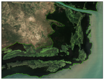 |
| Tiebuka Bay (ROI3) | 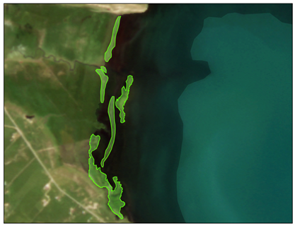 | 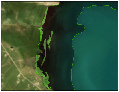 |
| Heima River inlet (ROI4) | 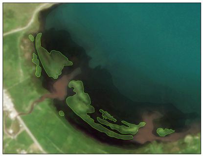 |  |
Disclaimer/Publisher’s Note: The statements, opinions and data contained in all publications are solely those of the individual author(s) and contributor(s) and not of MDPI and/or the editor(s). MDPI and/or the editor(s) disclaim responsibility for any injury to people or property resulting from any ideas, methods, instructions or products referred to in the content. |
© 2024 by the authors. Licensee MDPI, Basel, Switzerland. This article is an open access article distributed under the terms and conditions of the Creative Commons Attribution (CC BY) license (https://creativecommons.org/licenses/by/4.0/).
Share and Cite
Xu, W.; Shen, Q.; Zhang, B.; Yao, Y.; Zhou, Y.; Shi, J.; Zhang, Z.; Li, L.; Li, J. Remote Sensing Identification and Spatiotemporal Change Analysis of Cladophora with Different Morphologies. Remote Sens. 2024, 16, 602. https://doi.org/10.3390/rs16030602
Xu W, Shen Q, Zhang B, Yao Y, Zhou Y, Shi J, Zhang Z, Li L, Li J. Remote Sensing Identification and Spatiotemporal Change Analysis of Cladophora with Different Morphologies. Remote Sensing. 2024; 16(3):602. https://doi.org/10.3390/rs16030602
Chicago/Turabian StyleXu, Wenting, Qian Shen, Bo Zhang, Yue Yao, Yuting Zhou, Jiarui Shi, Zhijun Zhang, Liwei Li, and Junsheng Li. 2024. "Remote Sensing Identification and Spatiotemporal Change Analysis of Cladophora with Different Morphologies" Remote Sensing 16, no. 3: 602. https://doi.org/10.3390/rs16030602
APA StyleXu, W., Shen, Q., Zhang, B., Yao, Y., Zhou, Y., Shi, J., Zhang, Z., Li, L., & Li, J. (2024). Remote Sensing Identification and Spatiotemporal Change Analysis of Cladophora with Different Morphologies. Remote Sensing, 16(3), 602. https://doi.org/10.3390/rs16030602