Radar High-Resolution Range Profile Rejection Based on Deep Multi-Modal Support Vector Data Description

Abstract

Radar Automatic Target Recognition (RATR) based on high-resolution range profile (HRRP) has received intensive attention in recent years. In practice, RATR usually needs not only to recognize in-library samples but also to reject out-of-library samples. However, most rejection methods lack a specific and accurate description of the underlying distribution of HRRP, which limits the effectiveness of the rejection task. Therefore, this paper proposes a novel rejection method for HRRP, named Deep Multi-modal Support Vector Data Description (DMMSVDD). On the one hand, it forms a more compact rejection boundary with the Gaussian mixture model in consideration of the high-dimensional and multi-modal structure of HRRP. On the other hand, it captures the global temporal information and channel-dependent information with a dual attention module to gain more discriminative structured features, which are optimized jointly with the rejection boundary. In addition, a semi-supervised extension is proposed to refine the boundary with available out-of-library samples. Experimental results based on measured data show that the proposed methods demonstrate significant improvement in the HRRP rejection performance.

1. Introduction

Nowadays, radar realizes all-weather observation without relying on ambient radiation and is widely applied in remote sensing, such as ship detection and instance segmentation [1,2] and target tracking [3,4,5]. Radar Automatic Target Recognition (RATR) came into being to satisfy the growing demands of military surveillance, civil monitoring and environmental assessments. RATR is usually implemented based on high-resolution range profiles (HRRP) [6], synthetic aperture radar images [7,8,9], and inverse synthetic aperture radar images [10]. HRRP is more accessible and reflects physical structure information, such as the size of the target and the distribution of scattering points, which receives extensive attention in RATR [6]. The construction of a database containing complete target classes is the basis for RATR. However, it is incapable of guaranteeing the completeness of the HRRP database due to the difficulty of obtaining HRRPs of non-cooperative or even hostile targets in advance, like aircraft that mistakenly intrude and invade airspace. In such a situation, a false alarm or missed alarm will emerge when the target to be identified comes from an unknown class. Therefore, rejecting these targets before recognition, called out-of-library target rejection, is one of the most important yet difficult issues in the practical application of the RATR system.

The rejection task has the following unique problem complexities: (1) missing out-of-library samples are associated with unknown spatial distribution; and (2) the data structure of various in-library samples is complicated. The aforementioned problems give rise to several challenges in designing reasonable rejection models.

Conventional rejection models, such as One-Class Support Vector Machine (OC-SVM, [11]), Support Vector Data Description (SVDD, [12]), and Isolated Forest (IF, [13]), have been applied in the field of RATR. These models have relatively simple shallow structures and demonstrate stable rejection performance. However, the conventional rejection model can no longer accomplish the rejection task well due to the high-dimension and multi-modality characteristics of HRRP.

Deep learning has shown tremendous capabilities in learning expressive representations of such complexly distributed datasets, so deep rejection methods have been advancing to further satisfy practical requirements. Initially, well-trained neural networks are only used to extract features from high-dimensional samples, and then these features are fed into conventional rejection models [14,15]. Such hybrid methods exploit the powerful nonlinear mapping capability of deep networks and reduce the information loss in feature extraction. Nevertheless, they mostly ignore the unique and multi-modal distribution of HRRP. The optimization criteria for feature extraction and rejection boundary learning are usually inconsistent in two-phase procedures, resulting in extracting sub-optimal features for rejection [16]. Hence, many studies explore methods that can unify feature extraction with rejection models. The mainstream is divided into three categories, i.e., deep rejection methods based on reconstruction, self-supervised learning, and one-class classification. The first category has been proposed in the literature [17,18,19,20], which is inspired by the Auto-encoder (AE) and the Generative Adversarial Network. Such methods assume that in-library samples can be reconstructed well, so samples with larger reconstruction errors are rejected as out-of-library samples. Therefore, they usually regard reconstruction error as the rejection criterion and train a well-behaved generator of in-library samples. However, these methods are often irrespective of common features between in-library samples and out-of-library samples that benefit the reconstruction of out-of-library samples. Thus, they may be sub-optimal [16]. And they are weak in the utilization of multi-modal information of HRRP. Recently, self-supervised learning has been proven to be effective in feature extraction, and deep methods based on self-supervised learning have emerged endlessly [21,22,23]. Nevertheless, similar to the first category, most of them leave the latent overlap and multi-modality out of consideration. In addition, they usually have requirements for data types and are more suitable for image data [16]. Deep rejection methods based on one-class classification achieve an integrated design of feature extraction and rejection, such as Deep Support Vector Data Description (DSVDD, [24]). The core idea is similar to the traditional SVDD, with the difference that neural networks instead of kernel functions are leveraged to map in-library samples into a hyper-sphere in the feature space. And it outperforms conventional rejection methods and deep hybrid rejection methods. However, it assumes that all of the in-library samples follow the same distribution, which is unsuitable for describing the multi-modal structure of HRRP [25]. Therefore, Ghafoori et al. [25] embedded in-library samples into multiple hyper-spheres, but this still cannot effectively portray the anisotropic structure of HRRP and has limited performance on rejection.

To address the above problems, this paper proposes a novel rejection method for HRRP, named Deep Multi-modal Support Vector Data Description (DMMSVDD). It mainly contains a data preprocessor, a feature extractor with a dual attention module, and a rejector with a more compact rejection boundary. The data preprocessor aims to address the sensitivity problems specific to HRRP. The feature extractor with the dual attention module obtains distinguishing features with global temporal information and channel-dependent information. Based on the high-dimensional and multi-modal structure of HRRP, the rejector is competent to adaptively fit the complicated underlying distribution of in-library samples with an adjustable Gaussian mixture model (GMM). In the geometric sense, multiple closed hyper-ellipsoids are substituted for hyper-spheres in the existing SVDD-like methods design, which is conducive to constructing a tighter and more explicit rejection boundary. In the proposed method, the feature extraction and rejection boundary learning are jointly optimized under the unified distance-based rejection criterion. It can achieve a high matching between features and the rejection boundary and provide the foundation for improving rejection performance. Moreover, to deal with the situation in which limited out-of-library samples are available, a semi-supervised method is extended to tighten the rejection boundary with those out-of-library samples.

The contributions of this paper are summarized as follows:

• An efficient rejection method for HRRP is proposed, which jointly optimizes feature extraction and rejection boundary learning under a unified distance-based criterion;
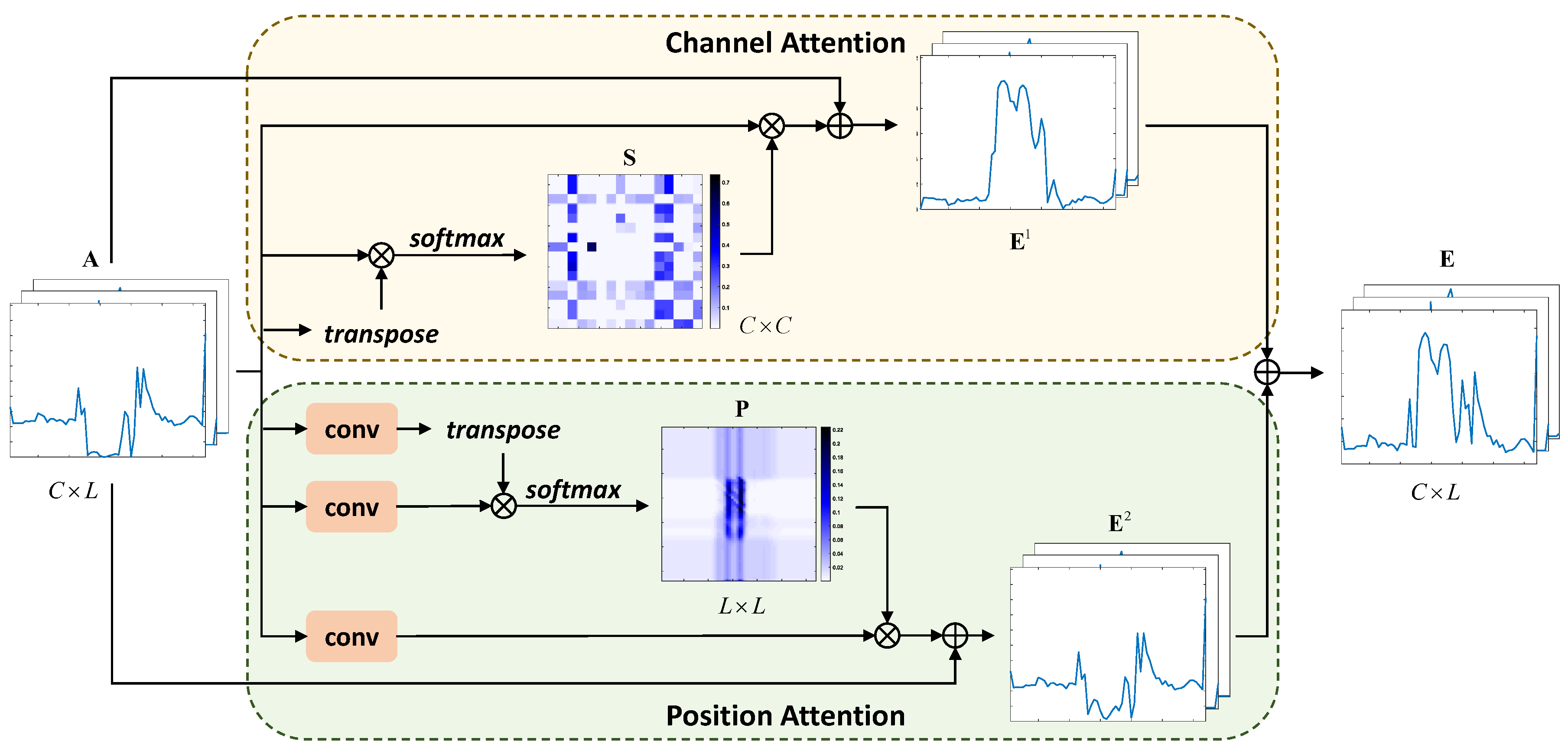
• The dual attention module in the feature extractor is capable of capturing the global and local structure information of HRRP, which further strengthens the feature discrimination between the in-library and out-of-library samples.
• Considering the high-dimensional and multi-modal structure of HRRP, a more compact and explicit rejection boundary is formed with an adjustable GMM;
• A semi-supervised method is extended to take advantage of available out-of-library samples to assist rejection boundary learning;
• Experiments demonstrate that the proposed methods can significantly promote the rejection performance on the measured HRRP dataset.

The rest of this paper is organized as follows: Section 2 describes the major related rejection methods; Section 3 provides the framework of the proposed methods; the experimental results are presented and analyzed in Section 4; and finally, Section 5 summarizes this paper.

2. Related Work

For the sake of notational uniformity, $x_n\in X(n=1,2,\cdots ,N)$ with $X\subset R^d$ denotes an in-library sample, where $N$ denotes the total number of in-library samples. This section provides a brief introduction to several typical rejection methods.

2.1. Support Vector Data Description

Inspired by the support vector classifier, Tax and Duin propose SVDD [12], in which in-library samples are mapped into a hyper-sphere by a kernel function in the feature space, whereas the projected out-of-library samples are located outside the hyper-sphere. The compactness of the hyper-sphere is guaranteed by minimizing the volume of the hyper-sphere, and the cost function of SVDD is as follows:

$$\begin{array}{l}\begin{array}{cc}\underset{R,c,\xi }{\min }& R^2+\frac{1}{vN}{\displaystyle \sum _{n=1}^N{\xi }_n}\end{array}\\ \begin{array}{cc}s.t.& \begin{array}{l}{‖\phi \left(x_n;o\right)-c‖}^2\le R^2+{\xi }_n\\ {\xi }_n\ge 0,n=1,2,\cdots N\end{array}\end{array}\end{array}$$

(1)

where $R$ and $c$ are the radius and center of the hyper-sphere in the feature space, respectively, $v$ is a penalty factor to balance the sample classification error with the complexity of the algorithm, ${\xi }_n$ is a relaxation factor, and $\phi \left(·;o\right)$ is a kernel function with a parameter $o$.

2.2. Deep Support Vector Data Description

DSVDD, proposed by Ruff et al. [24], employs neural networks to extract features instead of kernel functions in SVDD. The powerful expressiveness of neural networks breaks through the limitations of traditional kernel mapping and improves the differentiation between in-library and out-of-library samples in low-dimensional space. Similar to SVDD, it minimizes the volume of the hyper-sphere in the feature space so that the features of the in-library samples mapped by the neural network are contained inside the hyper-sphere as much as possible, while the features of the out-of-library samples are as far away from the hyper-sphere as possible, and the loss function of Deep SVDD is as follows.

$$\begin{array}{cc}\underset{R,W}{\min }& R^2+\frac{1}{vN}{\displaystyle \sum _{n=1}^N\max \left\{0,{‖\varphi \left(x_n;W\right)-c‖}^2-R^2\right\}}+\frac{\lambda }{2}{\displaystyle \sum _{l=1}^L{‖W^l‖}_F^2}\end{array}$$

(2)

where $\varphi \left(·;W\right)$ is a neural network with parameters $W$, $\lambda$ is a regularization parameter, $L$ is the number of network layers, and $W^l$ is l-th layer network parameters.

The training samples for the rejection task are mostly in-library samples, so this problem is ordinarily regarded as a one-class classification. Consequently, Ruff et al. [24] further simplify the above model by directly minimizing the mean distance between the features of training samples and the center, which is equivalent to minimizing the volume of the hyper-sphere.

$$\begin{array}{cc}\underset{W}{\min }& \frac{1}{N}{\displaystyle \sum _{n=1}^N{‖\varphi \left(x_n;W\right)-c‖}^2}+\frac{\lambda }{2}{\displaystyle \sum _{l=1}^L{‖W^l‖}_F^2}\end{array}$$

(3)

2.3. Deep Multi-Sphere Support Vector Data Description

Deep Multi-sphere Support Vector Data Description (DMSVDD) proposed by Ghafoori et al. [25] further improves the rejection performance by mapping in-library samples from different distributions to multiple hyper-spheres in the feature space.

$$\begin{array}{cc}\underset{W,R}{\min }& \frac{1}{K}{\displaystyle \sum _{k=1}^K{R}_k^2}+\frac{1}{vN}{\displaystyle \sum _{n=1}^N\max \left(0,{‖\varphi \left(x_n;W\right)-c_i‖}^2-R_i^2\right)}+\frac{\lambda }{2}{\displaystyle \sum _{l=1}^L{‖W^l‖}_F^2}\end{array}$$

(4)

where $K$ denotes the number of hyper-spheres in the feature space, and $R_k$ and $c_k$ denote the radius and center of the k-th hyper-sphere, respectively. $i={\mathrm{argmin}}_k{‖\varphi \left(x_n;W\right)-c_k‖}^2$.

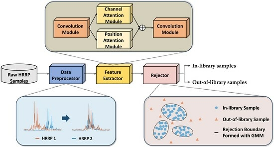
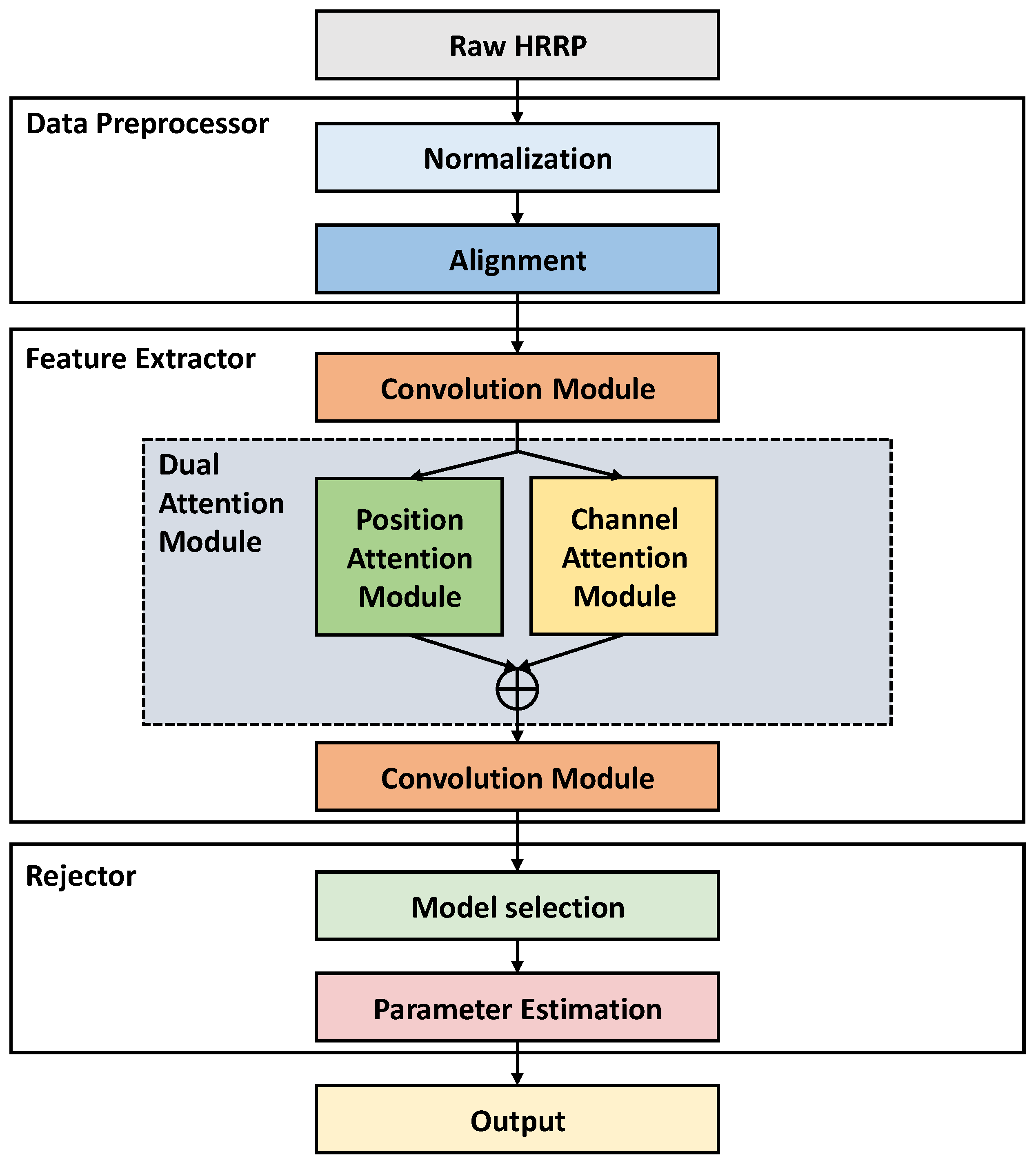
3. The Proposed Method

Considering the complex distribution of radar HRRP with high-dimension and multi-modality structure characteristics, this paper proposes a specific HRRP rejection method. As shown in Figure 1, the framework of the proposed method is mainly divided into a data preprocessor, a feature extractor, and a rejector. Firstly, data preprocessing alleviates the sensitivity problems of HRRP. Secondly, the convolution module and the dual attention module jointly realize the feature extraction of HRRP. The convolution module aims to extract the local spatial features of HRRP envelopes, and the dual attention module further obtains the global temporal and channel-dependent information ignored by the convolution module. Finally, the rejector fits the complex distribution of various in-library samples with the GMM. In-library samples are projected into multiple hyper-ellipsoids in the feature space, and out-of-library samples fall outside hyper-ellipsoids; therefore, a more delicate and closed rejection boundary is formed.

3.1. Data Preprocessor

Taking two HRRP samples as an example, the pre-processing procedure is shown in Figure 2. In particular, it mainly includes normalization and alignment, which alleviate the amplitude-scale and time-shift sensitivity of HRRP, respectively.

In practice, the received HRRP data contain amplitude information and phase information of targets, but the phase is greatly affected by the range variation. Hence, the phase of the target echo is usually ignored, and only the amplitude is preserved. Unfortunately, the amplitude is influenced by the radar antenna gain, target distance, target size, and other factors [26]. In order to alleviate the amplitude-scale sensitivity of HRRP, the L-2 normalization is usually used to erase the amplitude difference among samples and only retain their shape information. For an HRRP $\left\{x\left(r\right),r=1,2,\cdots ,R\right\}$, where $x\left(r\right)$ denotes the echo signal amplitude in the r-th range cell and $R$ denotes the number of range cells, its normalized result can be expressed as:

$$x^{\prime }\left(r\right)=\frac{x\left(r\right)}{\sqrt{{\displaystyle \sum _{u=1}^{R}x\left(u\right)}}},r=1,2,\cdots ,R$$

(5)

An HRRP is usually obtained by sliding the range window and intercepting part of the echo containing the target signal with a certain margin. As a result, the support area of the moving target may produce different degrees of shifting within the window. The center of gravity alignment is utilized to impair the impact of shifting support area on rejection [26]. Specifically, circular translation is operated to move the center of HRRPs to the center of gravity, i.e.,

$$G={\displaystyle {\sum }_{r=1}^{R}r{\left|x^{\prime }\left(r\right)\right|}^2}/{\displaystyle {\sum }_{r=1}^R{\left|x^{\prime }\left(r\right)\right|}^2}$$

(6)

3.2. Feature Extractor

The feature extraction network is divided into two convolution modules and a dual attention module. The convolution module can well reflect the local spatial information of targets [27]. A convolution module consists of several blocks, and one block includes a convolution layer, a batch-norm layer, a Leaky ReLU activation layer, and a pooling layer.

However, Ristea N C et al. [23] showed that stacked convolution layers aggregate low-level local features into high-level semantic features without comprehending the global arrangement. Specifically, given features from different channels, the convolution operation ignores their inter-dependencies and directly concatenates them. Given features from one channel, the convolution operation cannot acquire long-range dependency among all range cells of HRRP within the limitation of the local receptive field size. Attention modules have been widely applied in radar to solve the above-mentioned problems [28,29,30,31]. In this paper, the dual attention module [32] is added between convolution modules to further grasp the long-range and channel dependencies, respectively.

As illustrated in Figure 3, a dual attention module consists of a position attention module and a channel attention module.

The channel attention module adaptively recalibrates channel-wise features by a self-attention mechanism. Specifically, given a local feature $A\in R^{C\times L}$, where $C$ denotes convolution channels and $L$ denotes the feature dimensions, inter-dependencies among channels, called the channel attention map $S$, are calculated by applying a softmax layer to the matrix multiplication result of the transpose of $A$ and itself, i.e.,

$$s_{ij}=\frac{\exp \left(a_i·a_j\right)}{{\displaystyle {\sum }_{c=1}^C\exp \left(a_c·a_j\right)}}$$

(7)

where $s_{ij}$ denotes the impact of the $i$-th channel on the $j$-th channel, and $a_i$ denotes the feature of the $i$-th channel in the local feature $A$. Then, the feature $A$ and the channel attention map $S$ are matrix multiplied with a scale factor $\alpha$, and finally, the result is element-wise added with the local feature $A$ to obtain the feature map $E^1$, i.e.,

$$E_j^1=\alpha ·{\displaystyle \sum _{i=1}^C\left(s_{ij}{a}_i\right)}+a_j$$

(8)

where $E_j^1$ denotes the feature map of the j-th channel obtained by the channel attention module.

Differently, the position attention module first feeds $A$ into three convolutional layers to get three new feature maps $B\in R^{C\times L}$, $C\in R^{C\times L}$, and $D\in R^{C\times L}$. Then, the position attention map $P\in R^{L\times L}$ is computed by the feature map $B$ and $C$, i.e.,

$$p_{ij}=\frac{\exp \left(b_i·c_j\right)}{{\displaystyle {\sum }_{l=1}^L\exp \left(b_l·c_j\right)}}$$

(9)

where $p_{ij}$ denotes the impact of the i-th dimensional feature on the j-th dimensional feature, $b_i$ denotes the i-th dimensional feature of the feature map $B$, and $c_j$ denotes the j-th dimensional feature of the feature map $C$. The feature map $E^2$ is calculated as

$$E_j^2=\beta ·{\displaystyle \sum _{i=1}^L\left(p_{ij}{d}_i\right)}+a_j$$

(10)

where $E_j^2$ denotes the feature map of the j-th dimension obtained by the position attention module, and $d_i$ denotes the i-th dimensional feature of the feature map $D$.

The final feature map $E$ is a fusion of the $E^1$ from the channel attention module and $E^2$ from the position attention module. The dual attention module enables the support area of HRRP with plentiful target information to gain more attention and strengthens the feature discrimination. Moreover, the dynamic capture induces the affection of the shifting support area within HRRP on the rejection task.

3.3. Rejector

The key to rejecting out-of-library samples is to form an accurate distribution of in-library samples. The study [33] manifests that each range cell of HRRP is non-Gaussian and statistically correlated with others in high-dimensional space, which results in anisotropy and multi-modality characteristics of various in-library samples. Hence, it is unreasonable to curtly push them to obey one or several standardized Gaussian distributions. It is known that the GMM is competent at depicting the underlying distribution with the appropriate number of Gaussian components selected [34]. As shown in Figure 4, the left figure briefly depicts the probability distribution of HRRP, and the GMM with three components describes the distribution of in-library samples more accurately. In the geometric sense, the GMM fitting the in-library sample distribution means multiple closed hyper-ellipsoids wrapping in-library samples inside while excluding out-of-library samples outside. Compared with the other SVDD-like methods, the proposed method can better adapt to the non-uniformity and discontinuity of the in-library sample distribution. Note that a sample is considered to affect only one Gaussian component for efficiency. As for details of the structure selection and parameter estimation of the GMM, please refer to Section 3.5.

3.4. Objective Function

As mentioned above, we hope that the GMM can fit the distribution of in-library samples as closely as possible, which is interpreted in geometric terms to push the in-library samples into their nearest hyper-ellipsoids in the feature space as tightly as possible, so that out-of-library samples that deviate from this distribution are excluded from hyper-ellipsoids. Consequently, the goal of modeling the distributions turns to minimize the volume of every hyper-ellipsoid. Thus, the objective function is defined as:

$$\begin{array}{cc}\underset{\theta ,{\mu }_k,{\Sigma }_k,K}{\min }& \frac{1}{N}{\displaystyle \sum _{n=1}^N\underset{k=1,2,\cdots ,K}{\min }\left\{{\left(\varphi \left(x_n;\theta \right)-{\mu }_k\right)}^T{\Sigma }_k{ }^{-1}\left(\varphi \left(x_n;\theta \right)-{\mu }_k\right)\right\}}+\frac{\lambda }{2}{\displaystyle \sum _{p=1}^P{‖{\theta }^p‖}_F^2}\end{array}$$

(11)

where $\varphi (\cdot ;\theta )$ denotes the feature extractor with parameters $\theta$, $K$ denotes the number of Gaussian components, ${\mu }_k$ and ${\Sigma }_k$ denote the mean and covariance matrix of the k-th Gaussian component, respectively, $\lambda$ denotes a non-negative hyperparameter that controls the trade-off between compact loss and regularization, $P$ denotes the number of layers of the feature extractor, and ${\theta }^p$ denotes the p-th layer network parameters. The first term in (11) minimizes the volume of hyper-ellipsoids, and the second term ensures the generalization performance and lessens the risk of over-fitting.

The curse of rejection is that there is no prior knowledge about out-of-library samples. The rejection boundary only relies on limited in-library samples and could be inexplicit, which leads to insufficient rejection performance. To tackle the issue, it is urgent to exploit available out-of-library samples as much as possible. In recent years, semi-supervised rejection methods with outlier exposure [35,36,37] come into being. These methods attempt to regard out-of-library samples as negative samples to adjust the rejection boundary and obtain performance gains.

Based on DMMSVDD, we designed a semi-supervised method called Deep Multi-modal Semi-supervised Anomaly Detection (DMMSAD) for the HRRP rejection task. It makes use of the out-of-library samples to aid in learning a more explicit rejection boundary. The new objective function is defined as:

$$\begin{array}{cc}\underset{\theta ,{\mu }_k,{\Sigma }_k,K}{\min }& \begin{array}{l}\frac{1}{N+M}{\displaystyle \sum _{n=1}^N\underset{k=1,\cdots ,K}{\min }\left\{{\left(\varphi \left(x_n;\theta \right)-{\mu }_k\right)}^T{\Sigma }_k{ }^{-1}\left(\varphi \left(x_n;\theta \right)-{\mu }_k\right)\right\}}\\ +\frac{\eta }{N+M}{\displaystyle \sum _{m=1}^M{\left[\underset{s=1,\cdots ,K}{\min }\left\{{\left(\varphi \left({\tilde{x}}_m;\theta \right)-{\mu }_s\right)}^T{\Sigma }_s{ }^{-1}\left(\varphi \left({\tilde{x}}_m;\theta \right)-{\mu }_s\right)\right\}\right]}^{-1}}+\frac{\lambda }{2}{\displaystyle \sum _{p=1}^P{‖{\theta }^p‖}_F^2}\end{array}\end{array}$$

(12)

where ${\tilde{x}}_m$ denotes an out-of-library sample, $M$ denotes the total number of out-of-library samples, and $\eta$ denotes a non-negative hyperparameter that balances the effects of in-library and out-of-library samples on the boundary optimization. Compared with (11), the added term in (12) constrains out-of-library samples to be excluded from their nearest hyper-ellipsoids and further guarantees the compactness and clarity of the rejection boundary, as shown in Figure 5.

3.5. Training

The training procedure is explained in this section, including initializing and updating parameters.

3.5.1. Initializing

The initialization of the feature extractor parameters and the GMM parameters are described below.

• Initialization of feature extractor

The proposed method uses in-library samples for initializing, and the optimization may get stuck in local optima due to the lack of constraints on the distribution of out-of-library samples [38]. To improve the convergence, the network parameters are initialized with the AE, for which the structure is shown in Figure 6.

Assuming that $f_e(·):X\to Z$ is the encoder and $f_d(·):Z\to X$ is the decoder, both form an AE, where the encoder structure is consistent with the feature extractor structure. Given a sample $x_n\in X$, its reconstructed sample ${\hat{x}}_n$ is obtained by the AE, i.e.,

$${\hat{x}}_n=f_d\left(f_e\left(x_n;{\theta }_e\right);{\theta }_d\right)$$

(13)

where ${\theta }_e$ and ${\theta }_d$ denote the parameters of the encoder and decoder, respectively. During the training, the above AE is optimized using the mean square error as the loss function, i.e.,

$$\begin{array}{cc}\underset{{\theta }_e,{\theta }_d}{\min }& \frac{1}{N}{\displaystyle \sum _{n=1}^N{‖x_n-{\hat{x}}_n‖}_2^2}\end{array}$$

(14)

The training ends when the loss of AE converges. Then, the encoder parameters initialize the feature extractor parameters.

• Initialization of GMM

The parameters of GMM contain the number of Gaussian components $K$, the corresponding mean ${\mu }_k$, and the covariance matrix ${\Sigma }_k$ of each Gaussian component. The number of Gaussian components is selected empirically, and the mean and covariance matrix are initialized by K-means clustering [39].

3.5.2. Updating

Considering the different scales of the network parameters $\theta$, mean ${\mu }_k$ and covariance matrix ${\Sigma }_k$, it is difficult to update them directly using SGD [25], so we alternatively optimize Equation (11).

Step 1: Given the network parameters, the parameters of the GMM are optimized. Firstly, the number of Gaussian components of the GMM is selected. When the component number is too large, the redundant components could describe superfluous noise information and decrease the generalization performance. While the component number is too small, the GMM is incapable of delicately portraying the multi-modal distribution. Therefore, in order to select a fitted model structure, we adopt the ISODATA algorithm [40] to adaptively adjust the number of Gaussian components according to Equation (15).

$$K={\displaystyle {\sum }_{k=1}^K{1}_{\{n_k>=\nu ·\max \{n_1,n_2,\cdots ,n_K\left\}\right\}}}$$

(15)

where $n_k$ is the sample number corresponding to the k-th Gaussian components, and $\nu$ controls a fraction of hyper-ellipsoids to be abandoned. Secondly, the mean ${\mu }_k$ and covariance matrix ${\Sigma }_k$ are estimated using Gaussian mixture clustering [41].

Step 2: Parameters of the GMM are fixed, Equation (11) is optimized using the Adam optimizer [42], and the backpropagation algorithm updates the network parameters.

3.6. Theoretical Analysis

Essentially, parameter optimization is meant to maximize the log-likelihood of all samples in the Expectation-Maximization framework [43], regarding the GMM as latent variables. To be specific, the objective function is to maximize the log-likelihood of all samples, i.e.,

$$\begin{array}{cc}\max & {\displaystyle \sum _{n=1}^N\log p\left(x_n;\theta \right)}\end{array}$$

(16)

In the GMM, the objective function can be further expressed as

$$\begin{array}{cc}\max & {\displaystyle \sum _{n=1}^N{\displaystyle \sum _{k=1}^{K}p\left({\mu }_k,{\Sigma }_k;x_n,\theta \right)·\log p\left(x_n,{\mu }_k,{\Sigma }_k;\theta \right)}}\end{array}$$

(17)

E-step: Estimate the posterior probability $p({\mu }_k,{\Sigma }_k;x_n,\theta )$. Given the parameters of the GMM, we apply a hard shrinkage operation on the posterior probability, i.e.,

$$p({\mu }_k,{\Sigma }_k;x_n,\theta )=1_{k=i}$$

(18)

where $i=\underset{k}{\mathrm{argmin}}\{{(\varphi (x_n;\theta )-{\mu }_k)}^T{\Sigma }_k{ }^{-1}(\varphi (x_n;\theta )-{\mu }_k)\}$.

M-step: Maximize the log-likelihood. Under the assumption of a uniform prior over Gaussian components, we have

$$\begin{array}{cc}\hfill p\left(x_n,{\mu }_k,{\Sigma }_k;\theta \right)& =p\left(x_n;{\mu }_k,{\Sigma }_k,\theta \right)·p\left({\mu }_k,{\Sigma }_k;\theta \right)\hfill \\ & =\frac{1}{K}·\frac{1}{{\left(2\pi \right)}^{\frac{d}{2}}{\left|{\Sigma }_k\right|}^{\frac{1}{2}}}·\exp \left(-\frac{1}{2}{\left(\varphi \left(x_n;\theta \right)-{\mu }_k\right)}^T{\Sigma }_k^{-1}\left(\varphi \left(x_n;\theta \right)-{\mu }_k\right)\right)\hfill \end{array}$$

(19)

Substituting Equations (18) and (19) into (17) and ignoring the constant term, the objective function can be expressed as

$$\begin{array}{cc}\min & {\displaystyle \sum _{n=1}^N{\displaystyle \sum _{k=1}^K{1}_{k=i}\left[{\left(\varphi \left(x_n;\theta \right)-{\mu }_k\right)}^T{\Sigma }_k{ }^{-1}\left(\varphi \left(x_n;\theta \right)-{\mu }_k\right)\right]}}\end{array}$$

(20)

which is consistent with (11).

3.7. Rejection Criterion

In theory, in-library sample distribution fits closely, and the samples that deviate from the distribution are the out-of-library samples. Geometrically, the in-library samples are compactly wrapped inside hyper-ellipsoids in the feature space, while out-of-library samples fall outside. Therefore, the location of the test sample in the feature space can determine its category according to (21).

$$C\left(x\right)=\left\{\begin{array}{l}\mathrm{in}\text{-}\mathrm{library} \mathrm{samples}, \mathrm{dist}\left(x\right)<{\mathrm{dist}}_{\mathrm{threshold}}\\ \mathrm{out}\text{-}\mathrm{of}\text{-}\mathrm{library} \mathrm{samples}, \mathrm{otherwise}\end{array}\right.$$

(21)

where $\mathrm{dist}\left(x\right)=\underset{k=1,2,\cdots ,K}{\min }\left\{{\left(\varphi \left(x;\theta \right)-{\mu }_k\right)}^T{\Sigma }_k{ }^{-1}\left(\varphi \left(x;\theta \right)-{\mu }_k\right)\right\}$, and ${\mathrm{dist}}_{\mathrm{threshold}}$ denotes the distance threshold, which can be set according to the false alarm probability designed by the recognition system.

4. Results

In this section, we verify the rejection performance of proposed methods on the measured HRRP dataset. First, we briefly describe the details of the dataset. Then, implementation details are presented to ensure the reproduction of experiments. Next, we provide the definition and meaning of evaluation metrics. Finally, four experiments are conducted to exhibit the superior rejection performance of the proposed methods.

4.1. Dataset

The experimental radar transmits linear frequency modulation signals with a signal bandwidth of 400 MHz. The collected dataset consists of measured HRRPs of 10 types of aircraft targets. The training set contains 6000 HRRPs for every type, and the test set also contains 6000 HRRPs for every type. In order to verify the generalization performance of the method, the pitch angles of targets in the test set are slightly different from those in the training set.

4.2. Implementation Details

In this section, the performance of the proposed method is compared with conventional rejection methods and newly developed deep rejection methods. Traditional methods, including one-class SVM (OCSVM), isolated forest (IF), and kernel density estimation (KDE), and deep methods such as AE [44], VAE [45], MPN [46], HRN [47], NeuTraLAD [48], DSVDD, and DMSVDD, all use pre-processed HRRPs as inputs. The main structure and parameter settings of the feature extractor and decoder in the AE are shown in

Table 1. Main structure and parameter settings of our method.

	Module	Layer	Output Size	Normalization/Activation
Feature Extractor	Convolution Module 1	Conv1D	8 × 256	BN/Leaky ReLU
		Max Pooling	8 × 128	-
		Conv1D	16 × 128	BN/Leaky ReLU
		Max Pooling	16 × 64	-
	Dual Attention Module	Channel Attention	16 × 64	-
		Position Attention	16 × 64	-
	Convolution Module 2	Conv1D	8 × 64	BN/Leaky ReLU
		Max Pooling	8 × 32	-
		Flattening	1 × 256	-
		Conv1D	1 × 32	-
Decoder	Deconvolution Module 1	Reshape	2 × 16	-
		Upsample	2 × 32	-
		Deconv1D	8 × 32	BN/Leaky ReLU
		Upsample	8 × 64	-
		Deconv1D	16 × 64	BN/Leaky ReLU
		Upsample	16 × 128	-
	Dual Attention Module	Channel Attention	16 × 128	-
		Position Attention	16 × 128	-
	Deconvolution Module 2	Deconv1D	8 × 128	BN/Leaky ReLU
		Upsample	8 × 256	-
		Deconv1D	1 × 256	BN/Leaky ReLU
		Sigmoid	1 × 256	-

, and the encoder in the AE is consistent with the feature extractor. The initial number of Gaussian components is set to 10, and the hyperparameters $\eta$, $\lambda$, and $v$ are set to 0.1, 10⁻⁵, and 0.1, respectively. The learning rate of the Adam optimizer is set to 10⁻⁵. To be fair, we use the same convolution modules and deconvolution modules in other convolutional deep rejection methods.

4.3. Evaluation Metrics

In order to compare the rejection performance of different methods, we use the Receiver Operating Characteristics (ROC) curve and Area Under the Curve (AUC) for evaluation [24]. The ROC curve is obtained by plotting the true positive rate (TPR) versus the false positive rate (FPR), and they are defined as follows:

$$\begin{array}{l}\mathrm{TPR}=\frac{\mathrm{TP}}{\mathrm{TP}+\mathrm{FN}}\\ \mathrm{FPR}=\frac{\mathrm{FP}}{\mathrm{FP}+\mathrm{TN}}\end{array}$$

(22)

where $\mathrm{TP}$ denotes the total number of in-library samples being identified correctly in the test set, $\mathrm{FN}$ denotes the total number of in-library samples being misjudged, $\mathrm{FP}$ denotes the total number of out-of-library samples being misjudged, and $\mathrm{TN}$ denotes the total number of out-of-library samples being identified correctly. Obviously, the closer the ROC curve is to the upper left region, the larger the AUC and the better the rejection performance. In addition, following the previous works [48], we also use the F1-score as the evaluation indicator, which is calculated according to Equation (23), and the larger the F1-score, the better the rejection performance.

$$\begin{array}{l}\mathrm{Precision}=\frac{\mathrm{T}\mathrm{P}}{\mathrm{T}\mathrm{P}+\mathrm{F}\mathrm{P}}\\ \mathrm{Recall}=\frac{\mathrm{T}\mathrm{P}}{\mathrm{T}\mathrm{P}+\mathrm{F}\mathrm{N}}\\ {\mathrm{F}}_1=\frac{2·\mathrm{Precision}·\mathrm{Recall}}{\mathrm{Precision}+\mathrm{Recall}}\end{array}$$

(23)

4.4. Experiment with All Training Samples

In this section, we study how the methods deal with the HRRP rejection task. We randomly select 6 classes from 10 classes as in-library, and the remaining classes are treated as out-of-library. The above operations are repeated 4 times, corresponding to four experimental settings, and each experiment is repeated 10 times. Figure 7 shows the ROC curves of different methods, and

Table 2. AUC and F1-score of different methods under different experiment settings, with the best results bolded and the second-best underlined.

Method	AUC/F1-Score
	Setting I	Setting II	Setting III	Setting IV	Average
OCSVM	50.80/41.07	83.98/73.52	59.03/46.38	61.88/50.46	63.92/52.86
IF	52.62/43.31	80.58/63.59	54.91/45.22	51.82/42.66	59.98/48.70
KDE	47.06/38.10	81.88/69.66	53.91/41.40	55.67/45.38	59.63/48.64
AE	52.06/42.25	64.55/53.19	54.56/43.93	68.02/54.93	59.80/48.58
VAE	48.30/39.09	67.62/56.70	48.28/38.95	48.40/37.76	53.15/43.13
MPN	64.15/53.23	78.64/67.01	59.58/47.64	70.16/57.05	68.13/56.23
HRN	56.55/46.09	68.87/57.64	54.60/44.64	59.43/49.13	59.86/49.38
NeuTraLAD	62.96/51.18	81.55/68.28	56.25/45.45	65.60/53.39	66.59/54.58
DSVDD	62.82/51.08	82.07/69.46	67.32/55.10	66.69/54.76	69.73/57.60
DMSVDD	66.07/53.98	86.77/74.81	67.79/55.63	67.01/55.23	71.91/59.91
DMMSVDD (ours)	74.77/62.46	90.64/79.57	80.79/68.25	69.04/56.19	78.81/66.61
DMMSAD (ours)	75.41/62.39	91.16/81.09	81.01/68.50	76.03/64.00	80.90/68.99

gives the corresponding AUC and F1-score.

We can draw the following conclusions from the experiment results in Figure 7 and Table 2. Firstly, the rejection performance under the four settings is different. This means that the performance is associated with the classes of out-of-library samples, and some classes are difficult to reject. Secondly, the rejection performance of deep rejection methods is generally better than that of traditional methods. Limited by the shallow structure, features extracted by traditional methods, such as OCSVM, IF, and KDE, cannot effectively distinguish multi-class in-library samples and out-of-library samples. In contrast, deep rejection methods use neural networks to nonlinearly project high-dimensional samples to the feature space, where in-library samples are well separated from out-library samples. Finally, the results also illustrate the superiority of the proposed methods in most situations. As shown in Figure 7, the ROC curves of the proposed methods are closer to the upper left region, corresponding to larger AUC and F1-score in Table 2. In the HRRP rejection task, in-library samples are usually multi-class, which makes the multi-modal characteristic more prominent. MPN and NeuTraLAD aim to learn latent features of the in-library samples by data reconstruction or self-supervised learning, and HRN addresses the output bias to in-library samples with a gradient penalization. However, it weakens performance by neglecting the influence of multi-modal information on features. The reason for the decreasing performance of DSVDD and DMSVDD is that they restrict the in-library samples to obey the Gaussian distribution with zero mean and unit variance, which is obviously inconsistent with the multi-modality characteristic of in-library samples. The GMM in our methods fits closely to the complex distribution of multi-class in-library samples and tightens the rejection boundary. The dual attention module in the feature extractor optimizes the integration of convolutional features so that the support area of HRRP attracts more attention, which reflects the abundant physical structure information of the targets. Meanwhile, the dual attention module automatically focuses on the shifting target support area within HRRP and weakens the influence of the time-shift sensitivity on the performance to some extent. Furthermore, available out-of-library samples assist the optimization to a more explicit boundary, and the rejection of unknown out-of-library samples is more effective.

4.5. Experiment with Different Training Sample Sizes

Considering the difficulty of acquiring HRRPs in practice, the rejection performance of DMMSVDD is evaluated on several small sample sets without out-of-library samples. Four training sets are constituted from the aforementioned training set by uniform sampling, and the number of samples of each class target is 6000, 3000, 1500, and 750. For each training set, five classes are randomly selected as in-library targets, and the remaining classes are treated as out-of-library targets. The test set is kept constant. Each experiment is repeated 10 times, and

Table 3. AUC and F1-score of different methods with different training sample sizes, with the best results bolded and the second-best underlined.

Method	Training Sample Sizes (AUC/F1-Score)
	3750	7500	15,000	30,000
OCSVM	79.54/73.93	79.59/73.76	79.63/74.01	79.67/77.46
IF	75.91/71.32	76.07/71.41	76.15/71.45	76.18/71.54
KDE	75.50/71.72	75.79/71.98	75.80/72.01	75.83/73.76
AE	73.93/67.96	77.46/70.44	78.19/70.79	79.01/70.54
VAE	64.83/61.54	64.91/61.57	64.95/61.62	65.13/61.85
MPN	68.75/63.84	73.26/66.83	78.40/71.49	78.77/71.89
HRN	68.12/62.88	71.09/65.41	71.44/66.32	72.19/66.47
NeuTraLAD	78.26/71.14	78.49/71.58	79.01/71.76	79.26/71.93
DSVDD	78.00/71.54	78.19/71.68	78.85/72.09	81.25/74.16
DMSVDD	78.85/71.84	79.86/72.79	80.27/73.09	83.87/73.77
DMMSVDD (ours)	83.06/76.06	84.97/78.08	86.49/79.99	87.70/79.88

shows the AUC and F1-score of each method with different training sample sizes.

Traditional rejection methods work stably yet poorly, and the AUC of OCSVM, IF, and KDE remains at 79%, 76%, and 75%, respectively. Although their shallow structure does not require too many training samples to maintain performance, it limits the feature extraction ability of high-dimensional HRRP. As the training sample size decreases, the performance of most deep rejection methods weakens, but the proposed method still achieves remarkable performance. When the number of training samples drops from 30,000 to 3750, the AUC of AE, MPN, and DMSVDD declines to 73%, 68%, and 78%, respectively, whereas the AUC of DMMSVDD remains above 83%, which is the highest among all rejection methods. This is because the dual attention module grasps more comprehensive information and enhances feature discrimination by dynamically focusing on the HRRP support area. Moreover, the GMM characterizes the anisotropic and multi-modal structure of HRRP, which is beneficial to a more compact and delicate rejection boundary. In summary, the proposed method can cope with the HRRP rejection task in the case of a limited number of samples.

5. Discussion

In this section, we analyze the effectiveness of the proposed method by ablation study and visualization.

5.1. Ablation Study

The effectiveness of different components in the proposed method is evaluated in this section. The experimental setting is the same as in Section 4.4, and the results are shown in

Table 4. Impact of different modules on AUC, with the best results bolded and the second-best underlined.

Method	GMM	Channel Attention	Position Attention	Out-of-Library Samples	AUC
DMSVDD					66.07
DMSVDD-GMM	√				73.77
DMSVDD-GMMCA	√	√			74.22
DMMSVDD (ours)	√	√	√		74.77
DMMSAD (ours)	√	√	√	√	75.41

. The performance comparison between DMMSVDD and DMMSVDD-GMM verifies the significance of the rejection boundary formed with the GMM. DMSVDD-GMM eases restrictions of DMSVDD on the mean and covariance of the spatial distribution, which means the in-library samples are more compactly wrapped with multiple hyper-ellipsoids, then the rejection boundary tightens up. It significantly promotes the rejection performance, and the AUC increases from 66.07% to 73.77%. To quantify the effectiveness of the dual attention module, we add the channel attention module and the position attention module stage by stage to DMSVDD-GMM. Compared with DMSVDD-GMM, DMSVDD-GMMCA adopts the channel attention module, taking the dependency of different channel features into account. DMMSVDD further employs the position attention module, which obtains and utilizes the global temporal information among range cells within HRRP. Both attention modules enlarge the feature distinction between in-library and out-of-library samples and improve the performance. Further, the results of DMMSVDD and DMMSAD illustrate the rational leverage of out-of-library samples is indeed a simple but effective way for performance enhancement. The rejection boundary is more explicit with some out-of-library samples; therefore, the AUC of DMMSAD increases to 75.41%.

5.2. Visualization

5.2.1. Visualization of Separability

To demonstrate the feature extraction ability explicitly, Figure 8 visualizes the features of different methods. As these high-dimensional features are difficult to display directly, we visualize them by using the t-SNE [49] technique to reduce the dimension. The experimental setting is the same as in Section 4.4. Compared with other methods, features extracted by the proposed method show more regularity. The proposed method can obtain more compact features of multi-class in-library samples, while the features of other methods are relatively scattered. At the same time, there is less overlap between the features of in-library samples and out-of-library samples, so the proposed method can distinguish in-library samples well from out-of-library samples. This explains why the proposed methods outperform others.

5.2.2. Visualization of Position Attention Maps

To illustrate the effectiveness of the position attention module explicitly, Figure 9 visualizes measured HRRPs and the corresponding position attention maps of three types of targets with different sizes. The horizontal and vertical coordinates in measured HRRPs are range cell and magnitude, and the horizontal and vertical coordinates in position maps are both feature dimensions. Measured HRRPs in Figure 9 demonstrate that the wider target support area within an HRRP represents the larger actual size of the target. Obviously, the HRRP of target-A has the narrowest target support area, indicating that its actual size is the smallest, and the actual size of target-B and target-C is increasing. Figure 9 also shows the discrepancy among the position attention maps of three targets, with the relevant area in the position attention map of target-B being longer than that of target-A and shorter than that of target-C. In conclusion, the position attention map relates to the target support area within its HRRP, similarly reflecting the actual size of the target. The position attention module is capable of adaptively identifying the region where the target support area is located and assigning more weight to features in this region. It is conducive to strengthening the influence of the support area on the rejection performance and thus learning more discriminative features.

6. Conclusions

In this paper, a novel method named DMMSVDD is proposed to solve the HRRP-based rejection problem. The core ideas are to obtain more discriminative features with an attention module and form a more compact and explicit rejection boundary with the multi-modality of HRRP. Firstly, the data preprocessor is designed to alleviate the sensitivity problems of HRRP. Then, the feature extractor with a dual attention module is responsible for refining convolutional features with the global-dependency and channel-dependency information, which is effective in capturing abundant information in the support area of HRRP. Next, the rejector takes the anisotropy and multi-modality characteristics of HRRP into account and forms a more compact rejection boundary of multiple closed hyper-ellipsoids. The rejector is jointly optimized with the feature extractor under a unified rejection criterion. Moreover, its semi-supervised version, named DMMSAD, is extended to take advantage of out-of-library samples to obtain a more explicit boundary. Experiments demonstrate the promising performance of the proposed methods on the HRRP rejection task.

In applications, the HRRP database can be continuously expanded by merging accumulated out-of-library samples. And the users need to update the rejection model in a timely manner to improve the rejection performance. However, retraining a new rejection model every time is costly. Hence, in the future, we will introduce continual learning methods to update the existing model online based on newly acquired data, which is more efficient and cost-effective.

References

1. Zhang, T.; Zhang, X.; Liu, C.; Shi, J.; Wei, S.; Ahmad, I.; Zhan, X.; Zhou, Y.; Pan, D.; Li, J. Balance learning for ship detection from synthetic aperture radar remote sensing imagery. ISPRS J. Photogramm. 2021, 182, 190–207. [Google Scholar] [CrossRef]
2. Zhang, T.; Zhang, X. A mask attention interaction and scale enhancement network for SAR ship instance segmentation. IEEE Geosci. Remote Sens. Lett. 2022, 19, 4511005. [Google Scholar] [CrossRef]
3. Yan, J.; Jiao, H.; Pu, W.; Shi, C.; Dai, J.; Liu, H. Radar sensor network resource allocation for fused target tracking: A brief review. Inform. Fusion 2022, 86, 104–115. [Google Scholar] [CrossRef]
4. Yan, J.; Pu, W.; Zhou, S.; Liu, H.; Bao, Z. Collaborative detection and power allocation framework for target tracking in multiple radar system. Inform. Fusion 2020, 55, 173–183. [Google Scholar] [CrossRef]
5. Yang, Y.; Zheng, J.; Liu, H.; Ho, K.; Chen, Y.; Yang, Z. Optimal sensor placement for source tracking under synchronization offsets and sensor location errors with distance-dependent noises. Signal Process. 2022, 193, 108399. [Google Scholar] [CrossRef]
6. Liu, X.; Wang, L.; Bai, X. End-to-end radar HRRP target recognition based on integrated denoising and recognition network. Remote Sens. 2022, 14, 5254. [Google Scholar] [CrossRef]
7. Zhang, T.; Zhang, X. A polarization fusion network with geometric feature embedding for SAR ship classification. Pattern Recogn. 2022, 123, 108365. [Google Scholar] [CrossRef]
8. Zhang, T.; Zhang, X. Squeeze-and-excitation Laplacian pyramid network with dual-polarization feature fusion for ship classification in SAR images. IEEE Geosci. Remote Sens. Lett. 2021, 19, 4019905. [Google Scholar] [CrossRef]
9. Zhang, T.; Zhang, X. Injection of traditional hand-crafted features into modern CNN-based models for SAR ship classification: What, why, where, and how. Remote Sens. 2021, 13, 2091. [Google Scholar] [CrossRef]
10. Li, X.; Ran, J.; Wen, Y.; Wei, S.; Yang, W. MVFRnet: A novel high-accuracy network for ISAR air-target recognition via multi-view fusion. Remote Sens. 2023, 15, 3052. [Google Scholar] [CrossRef]
11. Schölkopf, B.; Platt, J.C.; Shawe-Taylor, J.; Smola, A.J.; Williamson, R.C. Estimating the support of a high-dimensional distribution. Neural Comput. 2001, 13, 1443–1471. [Google Scholar] [CrossRef]
12. Tax, D.M.; Duin, R.P. Support vector data description. Mach. Learn. 2004, 54, 45–66. [Google Scholar] [CrossRef]
13. Liu, F.T.; Ting, K.M.; Zhou, Z.-H. Isolation forest. In Proceedings of the Eighth IEEE International Conference on Data Mining, Pisa, Italy, 15–19 December 2008. [Google Scholar]
14. Erfani, S.M.; Rajasegarar, S.; Karunasekera, S.; Leckie, C. High-dimensional and large-scale anomaly detection using a linear one-class SVM with deep learning. Pattern Recogn. 2016, 58, 121–134. [Google Scholar] [CrossRef]
15. Andrews, J.; Tanay, T.; Morton, E.J.; Griffin, L.D. Transfer representation-learning for anomaly detection. In Proceedings of the 33rd International Conference on Machine Learning, New York, NY, USA, 20–22 June 2016. [Google Scholar]
16. Pang, G.; Shen, C.; Cao, L.; Hengel, A.V.D. Deep learning for anomaly detection: A review. ACM Comput. Surv. 2021, 54, 1–38. [Google Scholar] [CrossRef]
17. Perera, P.; Nallapati, R.; Xiang, B. OCGAN: One-class novelty detection using GANs with constrained latent representations. In Proceedings of the IEEE/CVF Conference on Computer Vision and Pattern Recognition, Long Beach, CA, USA, 15–20 June 2019. [Google Scholar]
18. Akcay, S.; Atapour-Abarghouei, A.; Breckon, T.P. GANomaly: Semi-supervised anomaly detection via adversarial training. In Proceedings of the 14th Asian Conference on Computer Vision, Perth, Australia, 2–6 December 2019. [Google Scholar]
19. Zaheer, M.Z.; Lee, J.-h.; Astrid, M.; Lee, S.-I. Old is gold: Redefining the adversarially learned one-class classifier training paradigm. In Proceedings of the IEEE/CVF Conference on Computer Vision and Pattern Recognition, Seattle, WA, USA, 13–19 June 2020. [Google Scholar]
20. Sabokrou, M.; Fathy, M.; Zhao, G.; Adeli, E. Deep end-to-end one-class classifier. IEEE Trans. Neur. Net. Lear. 2020, 32, 675–684. [Google Scholar] [CrossRef]
21. Golan, I.; El-Yaniv, R. Deep anomaly detection using geometric transformations. In Proceedings of the Advances in Neural Information Processing Systems, Montréal, QC, Canada, 3–8 December 2018. [Google Scholar]
22. Tack, J.; Mo, S.; Jeong, J.; Shin, J. CSI: Novelty detection via contrastive learning on distributionally shifted instances. In Proceedings of the Advances in Neural Information Processing Systems, Online, 6–12 December 2020. [Google Scholar]
23. Ristea, N.-C.; Madan, N.; Ionescu, R.T.; Nasrollahi, K.; Khan, F.S.; Moeslund, T.B.; Shah, M. Self-supervised predictive convolutional attentive block for anomaly detection. In Proceedings of the IEEE/CVF Conference on Computer Vision and Pattern Recognition, New Orleans, LA, USA, 18–24 June 2022. [Google Scholar]
24. Ruff, L.; Vandermeulen, R.; Goernitz, N.; Deecke, L.; Siddiqui, S.A.; Binder, A.; Müller, E.; Kloft, M. Deep one-class classification. In Proceedings of the International Conference on Machine Learning, Stockholm, Sweden, 10–15 July 2018. [Google Scholar]
25. Ghafoori, Z.; Leckie, C. Deep multi-sphere support vector data description. In Proceedings of the 2020 SIAM International Conference on Data Mining, Cincinnati, OH, USA, 7–9 May 2020. [Google Scholar]
26. Xia, Z.; Wang, P.; Dong, G.; Liu, H.J. Radar HRRP Open Set Recognition Based on Extreme Value Distribution. IEEE Trans. Geosci. Remote Sens. 2023, 61, 3257879. [Google Scholar] [CrossRef]
27. Chen, J.; Du, L.; Guo, G.; Yin, L.; Wei, D. Target-attentional CNN for radar automatic target recognition with HRRP. Signal Process 2022, 196, 108497. [Google Scholar] [CrossRef]
28. Zhang, T.; Zhang, X.; Shi, J.; Wei, S. HyperLi-Net: A hyper-light deep learning network for high-accurate and high-speed ship detection from synthetic aperture radar imagery. ISPRS J. Photogramm. 2020, 167, 123–153. [Google Scholar] [CrossRef]
29. Zhang, T.; Zhang, X.; Ke, X. Quad-FPN: A novel quad feature pyramid network for SAR ship detection. Remote Sens. 2021, 13, 2771. [Google Scholar] [CrossRef]
30. Zhang, T.; Zhang, X. A full-level context squeeze-and-excitation ROI extractor for SAR ship instance segmentation. IEEE Geosci. Remote Sens. Lett. 2022, 19, 4506705. [Google Scholar] [CrossRef]
31. Zhang, T.; Zhang, X.; Ke, X.; Liu, C.; Xu, X.; Zhan, X.; Wang, C.; Ahmad, I.; Zhou, Y.; Pan, D. HOG-ShipCLSNet: A novel deep learning network with hog feature fusion for SAR ship classification. IEEE Trans. Geosci. Remote Sens. 2021, 60, 1–22. [Google Scholar] [CrossRef]
32. Fu, J.; Liu, J.; Tian, H.; Li, Y.; Bao, Y.; Fang, Z.; Lu, H. Dual attention network for scene segmentation. In Proceedings of the IEEE/CVF Conference on Computer Vision and Pattern Recognition, Long Beach, CA, USA, 15–20 June 2019. [Google Scholar]
33. Wang, P.; Shi, L.; Du, L.; Liu, H.; Xu, L.; Bao, Z. Radar HRRP statistical recognition with temporal factor analysis by automatic Bayesian Ying-Yang harmony learning. Front. Electr. Electron. Eng. China 2011, 6, 300–317. [Google Scholar] [CrossRef]
34. Liu, H.; Du, L.; Wang, P.; Pan, M.; Bao, Z. Radar HRRP automatic target recognition: Algorithms and applications. In Proceedings of the 2011 IEEE CIE International Conference on Radar, Chengdu, China, 24–27 October 2011. [Google Scholar]
35. Hendrycks, D.; Mazeika, M.; Dietterich, T. Deep anomaly detection with outlier exposure. arXiv 2018, arXiv:1812.04606. [Google Scholar]
36. Ruff, L.; Vandermeulen, R.A.; Görnitz, N.; Binder, A.; Müller, E.; Müller, K.-R.; Kloft, M. Deep semi-supervised anomaly detection. arXiv 2019, arXiv:1906.02694. [Google Scholar]
37. Yao, X.; Li, R.; Zhang, J.; Sun, J.; Zhang, C. Explicit Boundary Guided Semi-Push-Pull Contrastive Learning for Supervised Anomaly Detection. In Proceedings of the IEEE/CVF Conference on Computer Vision and Pattern Recognition, Vancouver, BC, Canada, 17–24 June 2023; pp. 24490–24499. [Google Scholar]
38. Zaheer, M.Z.; Mahmood, A.; Khan, M.H.; Segu, M.; Yu, F.; Lee, S.-I. Generative cooperative learning for unsupervised video anomaly detection. In Proceedings of the IEEE/CVF Conference on Computer Vision and Pattern Recognition, New Orleans, LA, USA, 18–24 June 2022. [Google Scholar]
39. MacQueen, J. Some methods for classification and analysis of multivariate observations. In Proceedings of the Fifth Berkeley Symposium on Mathematical Statistics and Probability, Caliafornia, CA, USA, 21 June–18 July 1965 and 27 December 1965–7 January 1966. [Google Scholar]
40. Ball, G.H.; Hall, D.J. A clustering technique for summarizing multivariate data. Behav. Sci. 1967, 12, 153–155. [Google Scholar] [CrossRef] [PubMed]
41. Yang, M.-S.; Lai, C.-Y.; Lin, C.-Y. A robust EM clustering algorithm for Gaussian mixture models. Pattern Recogn. 2012, 45, 3950–3961. [Google Scholar] [CrossRef]
42. Kingma, D.P.; Ba, J. Adam: A method for stochastic optimization. arXiv 2014, arXiv:1412.6980. [Google Scholar]
43. Pernkopf, F.; Bouchaffra, D. Genetic-based EM algorithm for learning Gaussian mixture models. IEEE Trans. Pattern Anal. Mach. Intell. 2005, 27, 1344–1348. [Google Scholar] [CrossRef] [PubMed]
44. Masci, J.; Meier, U.; Cireşan, D.; Schmidhuber, J. Stacked convolutional auto-encoders for hierarchical feature extraction. In Proceedings of the 21st International Conference on Artificial Neural Networks, Espoo, Finland, 14–17 June 2011. [Google Scholar]
45. Kingma, D.P.; Welling, M. Auto-encoding variational bayes. arXiv 2013, arXiv:1312.6114. [Google Scholar]
46. Lv, H.; Chen, C.; Cui, Z.; Xu, C.; Li, Y.; Yang, J. Learning normal dynamics in videos with meta prototype network. In Proceedings of the IEEE/CVF Conference on Computer Vision and Pattern Recognition, Nashville, TN, USA, 20–25 June 2021. [Google Scholar]
47. Hu, W.; Wang, M.; Qin, Q.; Ma, J.; Liu, B. HRN: A holistic approach to one class learning. In Proceedings of the Advances in Neural Information Processing Systems, Online, 6–12 December 2020. [Google Scholar]
48. Qiu, C.; Pfrommer, T.; Kloft, M.; Mandt, S.; Rudolph, M. Neural transformation learning for deep anomaly detection beyond images. In Proceedings of the International Conference on Machine Learning, Virtual, 18–24 July 2021. [Google Scholar]
49. Van der Maaten, L.; Hinton, G. Visualizing non-metric similarities in multiple maps. Mach. Learn. 2012, 87, 33–55. [Google Scholar] [CrossRef]
Figure 1. The framework of the proposed method.
Remotesensing 16 00649 g001
Figure 2. HRRP pre-processing procedure.
Remotesensing 16 00649 g002
Figure 3. The details of the dual attention module.
Remotesensing 16 00649 g003
Figure 4. The design principle of the rejector and its geometric explanation.
Remotesensing 16 00649 g004
Figure 5. The geometric explanation of DMMSAD.
Remotesensing 16 00649 g005
Figure 6. The structure of AE.
Remotesensing 16 00649 g006
Figure 7. ROC curves of different methods under different experiment settings. (a) Experimental setting I; (b) experimental setting II; (c) experimental setting III; (d) experimental setting IV.
Remotesensing 16 00649 g007
Figure 8. The t-SNE visualization of different methods. The blue dots indicate the in-library sample features, and the yellow dots indicate the out-of-library sample features. (a) AE; (b) NeuTraLAD; (c) DSVDD; (d) DMSVDD; (e) DMMSVDD (ours); (f) DMMSAD (ours).
Remotesensing 16 00649 g008
Figure 9. Measured HRRPs and position attention maps of three types of aircraft targets with different sizes. (a) Target-A with small size; (b) target-B with medium size; (c) target-C with large size.
Remotesensing 16 00649 g009