Identification of O₃ Sensitivity to Secondary HCHO and NO₂ Measured by MAX-DOAS in Four Cities in China

Abstract

This study analyzed the differences in ozone (O₃) sensitivity in four different urban areas in China from February 2019 to January 2020 based on data on various near-surface pollutants from passive multi-axis differential optical absorption spectroscopy (MAX-DOAS) sites and nearby China National Environmental Monitoring Center (CNEMC) sites. Across the four cities, the nitrogen dioxide (NO₂) and formaldehyde (HCHO) concentrations varied seasonally. Xianghe consistently displayed the lowest NO₂ levels, suggesting reduced emissions compared to other cities. Guangzhou, a city with a robust economy and a high level of vehicle ownership, exhibited higher concentrations in spring. Summer brought elevated HCHO levels in Guangzhou, Xianghe, and Shenyang due to intensified photochemical processes. Autumn and winter showed higher HCHO concentrations in Guangzhou and Xianghe compared to Lanzhou and Shenyang. Overall, Guangzhou recorded the highest annual averages, due to its developed economy, while Xianghe’s lower NO₂ levels were offset by the elevated HCHO due to higher O₃ values. The analysis delved into primary and secondary HCHO sources across seasons and used carbon monoxide (CO) and O₃ data. Xianghe showcased the dominance of secondary sources in summer and autumn, while Lanzhou was characterized by primary dominance throughout the year. Shenyang mirrored Xianghe’s evolution due to industrial emissions. In Guangzhou, due to the high levels of vehicular traffic and sunlight conditions, secondary sources predominantly influenced HCHO concentrations. These findings highlight the interplay between primary and secondary emissions in diverse urban settings. This study explored O₃ sensitivity variations across seasons. Xianghe exhibited a balanced distribution among volatile organic compound (VOC)-limited conditions, nitrogen oxide (NO_x)-limited conditions, and transitional influences. Lanzhou was mainly affected by VOC-limited conditions in winter and NO_x-limited conditions in other seasons. Shenyang’s sensitivity varied with the seasons and was primarily influenced by transitions between VOCs and NO_x in autumn and NO_x-limited conditions otherwise. Guangzhou experienced varied influences. During periods of high O₃ pollution, all regions were affected by NO_x-limited conditions, indicating the necessity of NO_x monitoring in these areas, especially during summer in all regions and during autumn in Xianghe and Guangzhou.

1. Introduction

In recent years, air pollutant emissions have intensified in China. These pollutant emissions mainly include aerosols and ozone (O₃) [1,2]. Near-surface O₃ is mainly produced by precursor nitrogen oxides and volatile organic compounds in response to solar radiation [3], and it can damage the human respiratory system and vegetation. According to the 2021 World Health Organization air quality guidelines, regional long-term ozone pollution occurs when the peak season average concentration exceeds 60 µg/m³, while regional short-term ozone pollution occurs when the 8 h average concentration exceeds 100 µg/m³. According to the 2012 Technical Regulation on Ambient Air Quality Index of China, O₃ pollution in a region is classified as Class I if the 8 h average concentration exceeds 100 µg/m³ or the hourly concentration exceeds 160 µg/m³. It is classified as Class II if the 8 h average concentration exceeds 160 µg/m³ or the hourly concentration exceeds 200 µg/m³. Due to O₃’s complex formation mechanism, control of a single precursor cannot effectively control O₃ pollution [4]. Therefore, it is of great scientific significance to study O₃ sensitivity in different regions for the prevention and control of O₃ generation. However, O₃ tends to exhibit significant variations with the changing seasons [5]. Meanwhile, due to differences in economic and social development and living habits among different regions in China, the concentrations of atmospheric components show regional characteristics [6]. Therefore, it is generally necessary to compile and summarize data on the sensitivity of O₃ across different cities and seasons in an organized manner.

In previous studies, the ratio of formaldehyde (HCHO) and nitrogen dioxide (NO₂) columns in the troposphere was used to determine the sensitivity regime of O₃ formation [7]. HCHO is positively correlated with the formation of peroxy radicals and can be recognized as an indicator of total volatile organic compounds’ (VOCs) reactivity [8]. NO₂ is derived from transportation, industrial and residential use, power plants, etc. [9]. HCHO is not only the main indicator of VOCs but also a major precursor of O₃ and secondary organic aerosols (SOAs) near the surface [10,11]. There are two sources of HCHO. One type is mainly derived from direct emissions, referred to as primary sources, and the other is based on the photochemical oxidation process, referred to as secondary sources [12,13]. Strictly speaking, only the secondary source concentration of HCHO combined with NO₂ concentration can be used to analyze the sensitivity regime of O₃ formation [14]. Since the secondary source of HCHO is the main source of HCHO, many studies use the total HCHO to replace the secondary HCHO as the reactivity indicator of total VOCs [15]. However, in regions with more human activities, the contribution of the primary source of HCHO to the total HCHO cannot be ignored [16]. Therefore, the isolation of the secondary HCHO from HCHO is conducive to the analysis of the O₃ sensitivity mechanism in urban industrial areas.

In previous studies, the primary source, secondary source, and background source of HCHO were generally determined by multiple linear regression analysis [17,18]. The primary source of HCHO is strongly related to carbon monoxide (CO) emissions, while O₃ is strongly related to the secondary source generation of HCHO. Therefore, CO and O₃ are generally selected as tracers for primary and secondary sources of HCHO, and different sources of HCHO are separated by linear regression analysis [19,20]. In addition, some researchers have pointed out that it is more reasonable to use CO and glyoxal (CHOCHO) as tracers to separate the primary source and secondary source of HCHO, because the lifetimes of CHOCHO and HCHO in the atmosphere are similar [21]. Distinguishing the primary source and secondary source of HCHO can aid in quantitatively analyzing the relative contributions of air pollutants, such as industrial coal burning and motor vehicle exhaust, and provide a scientific basis for the formulation of emission reduction measures.

Since the concentrations of various atmospheric components vary at different times and in different regions, it is necessary to obtain long-term atmospheric component monitoring data in different regions through monitoring sites. At present, there are many methods used to obtain air pollutant concentration data worldwide. In China, the near-surface concentrations of O₃, CO, and NO₂ can be obtained from the China National Environmental Monitoring Center (CNEMC) [22]. The CNEMC has constructed pollutant monitoring sites throughout China which can perform long-term observations of the near-surface concentrations of various atmospheric components. Unfortunately, these sites do not have HCHO data. Passive multi-axis differential optical absorption spectroscopy (MAX-DOAS) is a detection method based on the characteristic absorption of trace gas molecules in the UV–visible band [23]. According to the position of the absorption peak and the intensity of the absorption line, it can identify and quantitatively analyze various gas components in the atmosphere. This method has many advantages, such as rapid detection, high sensitivity, a wide application range, and a high degree of automation; thus, it has been widely used [24].

This study delves into O₃ sensitivity in major industrial cities across China’s diverse regions and throughout the seasons. Ground-based MAX-DOAS monitoring stations were set up in Xianghe (representing the east), Lanzhou (west), Shenyang (north), and Guangzhou (south). We examined the diurnal and seasonal fluctuations in NO₂ and HCHO near the surface from February 2019 to January 2020. Utilizing O₃ and CO data from CNEMC sites, we distinguished the primary and secondary HCHO sources and scrutinized the near-surface O₃ sensitivity across these cities. The findings reveal the differences in O₃ generation, crucial for better pollution prevention and control. Section 2 and Section 3 detail the instrument setup, pollutant profile inversion, and data comparison among cities. To ensure accuracy, the NO₂ inversion results were validated with CNEMC data. Section 4 delineates the primary and secondary HCHO sources using MAX-DOAS and CNEMC data, analyzing O₃-NO_x-VOCs sensitivity in these areas.

2. Method and Methodology

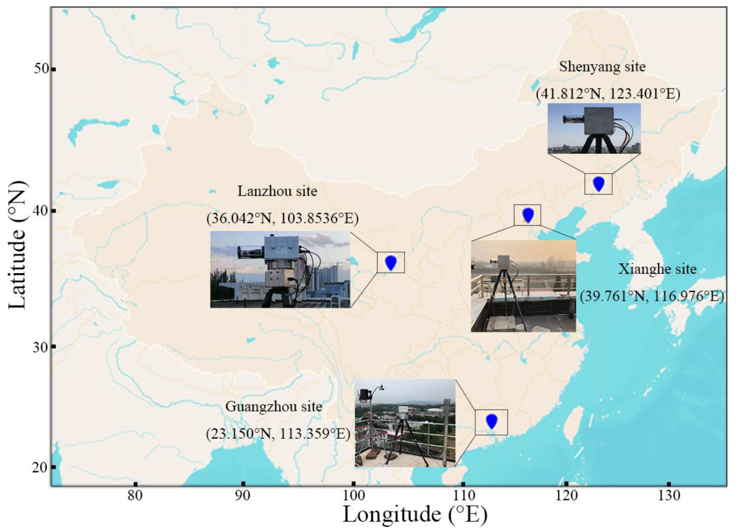
2.1. Instrument Setup

Ground-based MAX-DOAS is one important method in the field of atmospheric pollutant monitoring. It is based on the spectrum of solar scattered light received by the surface and can obtain the column concentration of trace gas in a rapid manner [23]. The University of Science and Technology of China (USTC) has built a ground-based remote sensing network of MAX-DOAS observation sites in many cities in China. It can realize long-term and online observations of the vertical structure of air pollution and haze pollution [25]. Through the observation results of each site, the vertical distribution of the concentration of atmospheric pollutants can be learned, providing insight into the transport of pollutants. To discuss the distribution differences of NO₂ and HCHO in different seasons and regions in China, typical metropolis measurement results from four regions were selected as representatives. In this study, the Xianghe site (39.761°N, 116.976°E) was selected as the eastern typical metropolis, the Lanzhou site (36.042°N, 103.854°E) was selected as the western typical metropolis, the Shenyang site (41.812°N, 123.401°E) was selected as the northern typical metropolis, and the Guangzhou site (23.150°N, 113.359°E) was selected as the southern typical metropolis. Figure 1 shows the location information for the MAX-DOAS in the four cities. Spectral instruments at each site were derived from the SkySpec-2D-210 system, which is manufactured by the Airyx company [26]. Detailed information for the instruments at the four sites is available in Appendix A and Table S1 in the Supplementary Materials. The telescope instrument performed observations at 10 elevation angles (1°, 2°, 3°, 4°, 5°, 8°, 10°, 15°, 30°, and a zenith angle of 90°), and each spectral data acquisition period was approximately 15 min. Spectral data detected at 8:00~16:00 during the daytime from January 2019 to February 2020 at the four sites were used to invert the vertical column concentrations of trace gases. The spectra collected by the instruments at each of the ground-based MAX-DOAS sites required the removal of noise in the spectrum—which includes the dark current (DC) and electronic offset—from the instruments themselves [23,27].

2.2. Spectral Analysis

All the measurement spectra were analyzed using the spectral analysis software QDOAS at http://uv-vis.aeronomie.be/software/QDOAS/ (accessed on 1 January 2024), which was developed at the Belgian Institute for Space Aeronomy (BIRA-IASB) [28]. Due to the influence of the working environment, there will be deviation between estimated wavelength and true wavelength; therefore, the high-resolution solar spectrum was used as the wavelength calibration file in the software [29]. In this study, the zenith spectrum (elevation angles = 90°) was used as the reference spectrum to retrieve the differential slant column densities (DSCDs). The DSCD is defined as the difference between the slant column density (SCD) of the measured spectrum and the corresponding zenith reference spectrum. The QDOAS software (version 3.4), based on the DOAS fitting method, uses the least squares method to obtain the SCDs of different atmospheric components [27]. A low-order polynomial ($\mathrm{P}\left(\lambda \right)=\sum b_k{\lambda }^k$) is added to the QDOAS software (version 3.4) fitting process to consider the contribution of broadband spectral structures (Rayleigh and Mie scattering) to the atmosphere. The inversion bands for NO₂ and HCHO are based on the ultraviolet ranges of 338.0–370.0 nm and 336.5–359.0 nm, respectively. All the required absorption cross-sections for the inversion of target pollutants are sourced from the UV–vis spectra website at https://uv-vis-spectral-atlas-mainz.org/uvvis/cross_sections/ (accessed 1 January 2024) [30].

Table 1. Inversion spectrum settings in the QDOAS software (version 3.4).

Parameter	NO2	HCHO
Wavelength range	338.0–370.0 nm	322.5–358.0 nm
NO2 (220 K) [32]	√	√
NO2 (298 K) [32]	√	√
O3 (223 K) [33]	√	√
O3 (243 K) [33]	√	√
O4 (293 K) [34]	√	√
BrO (223 K) [35]	√	√
HCHO (298 K) [36]	√	√
Ring spectrum [37]	By QDOAS	By QDOAS
Polynomial degree	5th order	5th order
Intensity offset	Constant	Constant

details the specific information required for the inversion of these two gases. With this method, we can obtain the SCD of the target pollutant. Usually, the SCD is highly dependent on the instrument’s observation mode and will be affected by the wavelength and different geometric parameters; thus, it is generally necessary to convert the SCD into vertical column densities (VCDs) via the air mass factor (AMF). The VCD represents the integral concentration of trace gas along the vertical path and is not affected by the geometric angle. In this study, we use the radiative transfer model to simulate the AMF required by MAX-DOAS inversion. The solution of the radiative transfer model used is SCIATRAN (version 2.2), which was developed by the Institute of Remote Sensing and the Institute of Environmental Physics of Bremen University [31]. When using SCIATRAN, users input parameters, such as aerosol properties, surface characteristics, temperature-pressure profiles, trace gas prior profiles, and observational geometric positions, into the input file to calculate and obtain the AMF.

2.3. Vertical Profile Retrieval

The information contained in the DSCD (measurement vector y) of multiple elevations in a scanning sequence from MAX-DOAS cannot be used to obtain a single solution of the profile, so the optimal estimation (OE) method and atmospheric radiative transfer model are needed to solve such problems in the actual calculation [38,39].

The essence of atmospheric inversion is to infer the atmospheric state vector x through the observation vector y, which can be expressed as in the following Equation (1) [40]:

$$y=F\left(x,b\right)+\epsilon$$

(1)

where y represents the O₄ or trace gas DSCD at various elevations obtained in a MAX-DOAS measurement cycle. O₄ is a relatively stable gas in the atmosphere, and the surface number density of O₄ is proportional to the square of the molecular oxygen (O₂) concentration [41]. Based on the number density of O₄, we can estimate the effective optical path of the MAX-DOAS instrument during observations [42]. Appendix B details the method for estimating an effective optical path based on O₄ SCD. x represents the aerosol extinction vertical profile or trace gas vertical profile, and b represents system parameters not involved in the inversion but affecting the measurement results (such as temperature and pressure profiles, albedo, single scattering albedo, asymmetry factor, etc.). F(x,b) represents the functional relationship between measurement vector y and atmospheric state vector x, and ε is the measurement error.

In the inversion of the OE method, the prior vector x_a is introduced, and the minimum value function χ²(x) is used to solve the optimal estimated state quantity x between the measurement information and the prior information to invert the real atmospheric state quantity [40]:

$${\chi }^2\left(x\right)={\left[F\right(x,b)-y]}^T{S}_{\epsilon }^{-1}\left[F\left(x,b\right)-y\right]+{[x-x_a]}^T{S}_a^{-1}[x-x_a]$$

(2)

where $x_a$ is the prior vector, containing the state vector of a priori information. S_ε is the covariance matrix of the measurement vector y, and the size is determined by the inversion results of the dependence of the measurement vector. S_a represents the covariance matrix of the prior vector $x_a$, and its magnitude reflects the dependence of the inversion results on the prior state vector. The inversion strategy is based on a Gauss–Newton (GN) scheme. Jacobians of $F\left(x,b\right)$, which describe the changes in the simulated DSCDs of each elevation angle, are used as a weighting function in this strategy [40].

In this study, to invert vertical profiles, we divided the atmospheric height into a sequence of 0 m, 100 m, 200 m, 300 m, 400 m, 500 m, 600 m, 700 m, 800 m, 900 m, 1000 m, 1200 m, 1400 m, 1600 m, 1800 m, 2000 m, 2200 m, 2400 m, 2600 m, 2800 m, and 3000 m. However, for the analysis of primary and secondary sources of near-surface formaldehyde and of ozone sensitivity, we mainly utilized trace gas results in the range of 0 to 100 m.

2.4. Regression Model for Source Separation in Ambient HCHO

There are two main HCHO sources of pollution in the atmosphere: one type arises mainly from the combustion of fossil fuels, which is referred to as the primary source, and the other arises mainly from the photochemical oxidation process in the atmosphere, which is referred to as the secondary source. In this study, the contributions of the primary and secondary sources are distinguished based on the use of source tracers. This was based on the method proposed by Ma et al.: CO is used as the primary source tracer and O₃ as the secondary source tracer [16,43,44,45,46]. The contributions of primary sources, secondary sources, and background sources to atmospheric HCHO are preliminarily calculated based on a multiple regression model, and the equation is as follows:

$$\left[HCHO\right]={\beta }_0+{\beta }_1\times \left[C_{\mathrm{C}\mathrm{O}}\right]+{\beta }_2\times \left[C_{{\mathrm{O}}_3}\right]$$

(3)

where β₀ represents the background value of HCHO in the atmospheric environment, and ${\beta }_1\times \left[C_{\mathrm{C}\mathrm{O}}\right]$ represents the primary source of HCHO. This means that an increase of one unit of CO will increase the HCHO concentration of the β₁ unit accordingly. ${\beta }_2\times \left[C_{{\mathrm{O}}_3}\right]$ represents the secondary source of HCHO, which means that an increase of one unit of CO will increase the HCHO concentration of β₂ units accordingly. Thus, the primary and secondary sources of HCHO in the four cities can be obtained. The specific formula is as follows:

$$P_{primary}=\frac{{\beta }_1\times \left[C_{\mathrm{C}\mathrm{O}}\right]}{{\beta }_0+{\beta }_1\times \left[C_{\mathrm{C}\mathrm{O}}\right]+{\beta }_2\times \left[C_{{\mathrm{O}}_3}\right]}\times 100\%$$

(4)

$$P_{secondary}=\frac{{\beta }_2\times \left[C_{{\mathrm{O}}_3}\right]}{{\beta }_0+{\beta }_1\times \left[C_{\mathrm{C}\mathrm{O}}\right]+{\beta }_2\times \left[C_{{\mathrm{O}}_3}\right]}\times 100\%$$

(5)

$$P_{background}=\frac{{\beta }_0}{{\beta }_0+{\beta }_1\times \left[C_{\mathrm{C}\mathrm{O}}\right]+{\beta }_2\times \left[C_{{\mathrm{O}}_3}\right]}\times 100\%$$

(6)

Through this regression model, we can distinguish between the concentrations of primary and secondary sources of HCHO in the environment.

2.5. Methodology for O₃ Sensitivity Analysis

At present, a common method to determine O₃ sensitivity is through the ratio of HCHO/NO₂ [47]. The determination index $f_{regime}$ is defined as follows [48]:

$$f_{regime}=c_{\mathrm{H}\mathrm{C}\mathrm{H}\mathrm{O}}/c_{{\mathrm{N}\mathrm{O}}_2}$$

(7)

Under different HCHO/NO₂ ratios, linear fitting is performed for O₃ and the normalized HCHO and NO₂ concentrations. After enumerating the threshold range during each layer observation period and constantly reducing the upper and lower limits of the threshold, the index meets the threshold upper limit $f_1$ and threshold lower limit $f_2$. When $f_{regime}$ < $f_1$, O₃ generation is considered to be VOC limited. When the index is $f_{gime}$ > $f_2$, O₃ generation is considered to be NO_x limited. When $f_1$ < $f_{regime}$ < $f_2$, O₃ generation is considered to be transitional between VOCs and NO_x.

2.6. Ancillary Data

In this study, to verify the accuracy of the inverted data, the results of NO₂ are directly compared with the data from the nearest sites of the CNEMC website https://air.cnemc.cn:18007/ (accessed on 1 January 2024). The CNEMC has set up ground-based sites, in various cities in China, which measure the near-ground concentrations of various atmospheric trace gases with in situ chemical point instruments. The CNEMC records the concentration values of atmospheric components every hour. Since the CNEMC sites are all in situ measuring instruments, they can only obtain the near-surface trace gas concentration. Therefore, this study compares the concentration at the bottom of the profile with the results from the CNEMC sites. Meanwhile, near-surface O₃ and CO₂ data were also obtained from the CNEMC sites. To ensure uniformity in the subsequent calculations, we were required to transform the data from the CNEMC sites. At near-surface standard pressure (1 atm), the conversion relationship between units of mass per volume (μg/m³) and parts per billion by volume (ppb) can be approximately calculated using the following Equation (8) [49,50]:

$$\mathsf{\mu }\mathrm{g}/{\mathrm{m}}^3=\frac{\left(\mathrm{p}\mathrm{p}\mathrm{b}\right)·\left(12.187\right)\ast \left(M\right)}{273.15+°\mathrm{C}}$$

(8)

where $M$ represents the relative molecular mass of the trace gas.

3. Results

In this section, we show the profile results obtained by the OE method. We verify the NO₂ near-surface results in four cities by comparing them with the data of the CNEMC sites in the same period. Then, we provide the NO₂ and HCHO profile results of the four cities in different seasons and analyze the similarities and differences between the NO₂ and HCHO profile results in the four cities. This section analyzes the distribution characteristics of polluted gases at the four sites based on the MAX-DOAS ground-based instrument’s measurements across one year (measurement time: February 2019–January 2020). Since MAX-DOAS observation can only be carried out in the daytime, we mainly analyze the variations in pollutant gases during this period (8:00~16:00).

3.1. Verification of MAX-DOAS Results

Based on the method in Section 2.3, we obtained the NO₂ and HCHO vertical profile information of four MAX-DOAS sites. Since the CNEMC sites do not provide hourly HCHO concentration results, this study mainly compares the near-surface NO₂ results of the vertical profiles (0–100 m) of the four MAX-DOAS sites with the nearest CNEMC site’s results.

Table 2. CNEMC sites within the MAX-DOAS observation direction.

	Nearest CNEMC Site Name	Longitude	Latitude	Distance from MAX-DOAS Instrument
Xianghe	Development Zone	116.7729°E	39.5747°N	3.0592 km
Lanzhou	Railway Design Institute	103.8310°E	36.0464°N	2.5557 km
Shenyang	Taiyuan Street	123.3997°E	41.7972°N	1.6491 km
Guangzhou	Tiyu West Street	113.3208°E	23.132 °N	4.6733 km

shows the information of the nearest CNEMC sites to the four MAX-DOAS sites. To enhance the reliability of our results, we applied a rigorous filtration process to the trace gas data. Here, we primarily referred to Wang’s paper and applied the following criteria for filtering: excluding data with solar zenith angle (SZA) > 85°, root-mean square (RMS) < 2 × 10⁻³, deviations of modeled and measured dSCD < 1 × 10¹⁶ molecules/cm⁻², relative intensity offset (RIO) in the DOAS fit < 1%, and excluding data under thick cloudy conditions [51]. Additionally, to account for variations in SZA throughout the year and across different regions, we consistently selected results within the timeframe of 8:00 to 16:00. Figure S1 in the Supplementary Materials illustrates the average diurnal variations of SZA for the four sites in different seasons.

Figure 2A–D show the correlation test results of the NO₂ near-surface concentration obtained through the OE algorithm and corresponding CNEMC sites at the four MAX-DOAS sites. Figure 2A–D show that the correlation coefficients of the hourly NO₂ results of the four MAX-DOAS sites and the corresponding CNEMC sites reach 0.732, 0.806, 0.812, and 0.751, respectively. The near-surface NO₂ concentrations at the four sites exhibit evolution in time consistent with the NO₂ concentrations observed at the CNEMC site. The correlation coefficient of the comparison results between the Guangzhou site and Xianghe site is lower than that between the Lanzhou site and Shenyang site. This possibly occurs because the distance between each of the four sites and the corresponding CNEMC site is different. In general, the correlation coefficient between the results of two sites that are closer to each other is better. The slope values for the linear regression analysis in Xianghe, Lanzhou, Shenyang, and Guangzhou are 0.996, 0.806, 1.083, and 0.617, respectively. Correspondingly, the intercepts are 11.286, 31.881, 13.833, and 17.784. There are many reasons for this. First, the spectrum captured by the MAX-DOAS instrument differs from the environment observed by the in situ instrument. In situ instruments mainly obtain the NO₂ concentration in the nearby range, while MAX-DOAS obtains the environmental information in the effective optical path in one direction [24]. According to the method outlined in Appendix B, under clear sky conditions, the UV effective optical path calculated using O₄ SCD for the MAX-DOAS instrument we used is approximately 5–9 km. Secondly, there is a systematic error between the method of retrieving the SCD and the gas concentration obtained by the in situ instrument [52]. Tirpitz et al. discusses that the systematic errors in MAX-DOAS SCD primarily stem from uncertainties in cross-sections of the literature, instrumental effects, or simplifying assumptions made during DOAS spectral analysis [53]. Finally, the OE algorithm may produce certain calculation errors when calculating the MAX-DOAS profile due to prior information and the number of iterations [54,55,56]. These errors will lead to direct differences between the two results.

3.2. Vertical Structural Differences in NO₂ and HCHO among the Four Cities

Using the atmospheric pollutant profile obtained from the inversion results, this section discusses the differences in and causes of the vertical profiles of trace gases based on the comparison of different seasons in the four cities.

Figure 3 shows the profile of the average NO₂ concentration in the four cities in different seasons. Due to the influence of the shape of the a priori concentration distribution, the NO₂ concentration profiles in all four regions exhibit an exponential decrease from the ground upward. From Figure 3, the concentration of NO₂ in Xianghe is the lowest in all four seasons, which proves that the total amount of NO₂ gas emissions in Xianghe is lower than that in other cities in all seasons of the year. Among the four cities, Guangzhou’s economy is more developed, and its level of motor vehicle ownership is the highest across China. Therefore, the concentration of NO₂ in Guangzhou is higher than that in the other three cities in spring. In summer, due to the influence of the monsoon, clean air entering the mainland from the ocean will dilute the NO₂ in the troposphere in the Pearl River Delta region. Therefore, the concentrations of NO₂ in Lanzhou, Shenyang, and Guangzhou are relatively similar in summer. In autumn, the level of NO₂ in Lanzhou is the highest among the four cities, which may be due to the influence of natural sources and weather in the inland area in autumn. Organisms are active in autumn and easily produce NO₂. At the same time, the climate is dry in autumn and has a weak effect on the deposition and dilution of atmospheric pollutants. However, Shenyang and Guangzhou are close to the ocean and still experience the rainy season at this time, which dilutes and purifies the NO₂ in the atmosphere. However, the weather in winter itself is milder, which easily increases the air pollution. Lanzhou and Shenyang, as provincial capitals, experience increased coal burning when they enter the heating season, while the motor vehicles used in Guangzhou emit more exhaust gas. Therefore, the concentration of NO₂ in these three cities is high.

Figure 4 shows the profile of the average HCHO concentration in the four cities in different seasons. Overall, similar to NO₂, the concentration profiles of HCHO gradually decrease from low to high altitudes. However, during spring, summer, and autumn in Guangzhou, as well as during summer in Shenyang and Lanzhou, there are elevated levels of HCHO observed at altitudes between 200 m and 400 m. This is primarily due to the photochemical reactions of volatile organic compounds in favorable sunlight conditions at lower altitudes, resulting in the formation of HCHO [57]. In spring, the highest HCHO concentration is obtained in Guangzhou. NO₂ is the primary source of HCHO generation, and the large number of vehicles used in Guangzhou emit NO₂ tail gas; thus, the concentration of HCHO in Guangzhou increases. However, the HCHO concentration in the Xianghe area is higher than that in Shenyang and Lanzhou, which may be due to the high values of O₃ in the Xianghe area during the MAX-DOAS normal observation period (Figure S2 in the Supplementary Materials). O₃ is the secondary source of HCHO; therefore, the HCHO concentration in the Xianghe area increases. In summer, the photochemical oxidation process occurs more easily due to the increase in light intensity, so the HCHO concentrations in Guangzhou, Xianghe, and Shenyang all show a notable increase. However, Lanzhou, as a city in the western region with less vegetation and lower anthropogenic activity compared to the other three cities, exhibits the lowest HCHO concentration among them during the summer. In autumn, the evolution of the HCHO concentration in the four cities is similar to that in spring, with Guangzhou showing the highest, Xianghe the second highest, and Lanzhou and Shenyang the lowest levels. In winter, the concentration of HCHO in Guangzhou is higher than that in the other three cities due to the strong illumination in the south and the greater vehicle exhaust emissions in Guangzhou. Meanwhile, in the other three cities, it is difficult for the transformation process of HCHO to take place due to the low light levels in winter and insignificant change in temperature.

Overall, from an annual average perspective, the near-surface NO₂ and HCHO concentration are the highest in Guangzhou. Guangzhou is one of the most developed cities in China, and the concentrations of NO₂ and HCHO emitted by industry are also higher. Shenyang and Lanzhou are both provincial capitals in the north, and their industrial areas and living habits are similar, to some extent, which makes their yearly mean vertical profiles of NO₂ and HCHO similar. The near-surface NO₂ concentration in Xianghe City is the lowest, which may be caused by the overall low emissions of industrial combustion and automobile exhaust in Xianghe. Additionally, the overall O₃ concentration in the Xianghe area is high, and the air circulates relatively well, resulting in many photochemical oxidation processes occurring in Xianghe. This may be the reason that the near-surface HCHO concentration in Xianghe is higher than that in Lanzhou and Shenyang.

3.3. Detailed Overview of NO₂ and HCHO in Four Cities

Based on the inversion results, the diurnal variation characteristics of NO₂ and HCHO in the four cities are summarized in the following section.

Figure 5A–D and Figure 6A–D show the vertical average concentration profiles of NO₂ and HCHO from 8 to 16 o’clock in different seasons in Xianghe. From Figure 5A–D, it can be observed that the vertical profile of NO₂ concentrations in Xianghe is at its lowest during summer, with a near-surface average NO₂ concentration of approximately 4.795 ppb, and it is highest during winter, with a near-surface average NO₂ concentration of approximately 8.789 ppb, while the values for spring and autumn lie between these extremes. The increased use of coal, oil, and other fuels for heating during winter contributes to higher NO₂ emissions. Additionally, the weaker solar radiation and lower atmospheric temperatures in winter prolong the lifespan of NO₂. Conversely, the stronger sunlight in summer facilitates NO₂ photolysis. Across the seasons, the overall evolution in time for spring and summer shows higher NO₂ concentrations in the morning and lower concentrations in the afternoon, attributed to increased sunlight in the afternoon, accelerating NO₂ photolysis. In contrast, during autumn, the NO₂ concentrations are higher in the morning and evening but lower at midday due to the reduced sunlight duration, leading to elevated NO₂ values in the early morning and evening. In winter, the NO₂ concentrations exhibit relatively stable diurnal variations. With lower atmospheric boundary layers and the frequent occurrence of temperature inversions in Xianghe during winter, NO₂ tends to accumulate in the lower atmosphere, persisting for longer periods within the troposphere [58,59,60].

Figure 6A–D show that Xianghe’s highest HCHO concentration occurs during summer, with a near-surface average HCHO concentration of approximately 6.126 ppb, followed by autumn, with a near-surface average HCHO concentration of approximately 3.999 ppb. Conversely, the HCHO concentrations are lowest during spring and winter, with near-surface average HCHO concentrations of approximately 2.868 ppb and 2.492 ppb, respectively. During summer, the atmospheric photochemical oxidation process primarily influences the HCHO value. Alkanes, alkenes, and benzene derivatives can serve as precursors for HCHO through atmospheric photochemical processes [61,62,63]. These precursors, originating from both natural emissions and anthropogenic sources, undergo complex reactions with O₃, nitrogen oxide (NO_x), and hydroxyl (OH) radicals, leading to the formation of photochemical smog and, consequently, generating greater quantities of oxygenated compounds such as HCHO.

Figure 5E–H and Figure 6E–H show the vertical average concentration profiles of NO₂ and HCHO from 8 to 16 o’clock in different seasons in Lanzhou. From Figure 5E–H, the lowest concentrations are observed in summer, with a daytime average near-surface concentration of approximately 10.372 ppb; it increases slightly in spring, to an average of approximately 14.613 ppb during the day. However, it peaks in autumn and winter, reaching near-surface daytime average concentrations of around 24.339 ppb and 25.395 ppb, respectively. During spring and summer in Lanzhou, the NO₂ concentrations tend to be higher before noon and decrease in the afternoon due to higher temperatures and longer daylight hours. With stronger sunlight around midday, NO₂ readily undergoes photochemical reactions with VOCs in the ambient air, leading to the generation of O₃. In contrast, the lower temperatures during autumn and winter reduce the reactivity of NO₂. Coupled with unfavorable meteorological conditions hindering pollutant dispersion, this results in higher NO₂ concentrations during these seasons, with a relatively stable daytime pattern.

Figure 6E–H show that the HCHO concentrations in Lanzhou show relatively insignificant differences among the four seasons, with daytime average near-surface HCHO concentrations ranging between approximately 2.675 ppb and 3.725 ppb. There is a slight increase in the near-surface HCHO concentration during autumn and winter in Lanzhou, but these results are unusual. There could be multiple reasons for them. First, in the western regions, during autumn and winter, severe haze conditions, especially in winter due to atmospheric transmission processes, often carry higher values of HCHO pollution [64,65]. Second, chemical combustion during the heating season in winter in these western areas might contribute to the production of HCHO. Third, the lower temperatures during autumn and winter can prolong the survival time of HCHO in the air, reducing its volatility.

Figure 5I–L and Figure 6I–L show the vertical average concentration profiles of NO₂ and HCHO from 8 to 16 o’clock in different seasons in Shenyang. From Figure 5I–L, it is evident that, overall, the NO₂ concentrations in Shenyang are highest during winter, with a daytime average near-surface concentration of approximately 17.758 ppb, and lowest during summer, with a daytime average near-surface concentration of approximately 9.635 ppb. The higher NO₂ value in the morning during spring and summer might be due to human activities at this time. However, during midday and the afternoon in spring and summer, the NO₂ concentrations gradually decrease. Due to the smaller SZA (Figure S1 in the Supplementary Materials) in spring and summer compared to autumn and winter, more intense sunlight is present. This enhanced sunlight contributes to the photochemical depletion or atmospheric dilution of NO₂. In autumn and winter, the peaks in NO₂ concentration mainly occur in the early morning and evening. This could be attributed to the shorter daylight hours in the northern winter and earlier off-work hours, causing peak traffic emissions during these times. Additionally, in winter, Shenyang experiences the heating season, with significant coal combustion contributing to substantial amounts of NO₂ emissions.

Figure 6I–L show that the HCHO concentration in Shenyang peaks during summer, with a daytime average near-surface concentration of approximately 3.907 ppb, while the daytime average near-surface concentrations are lower in the other three seasons. During summer, the daytime variation in HCHO exhibits a continuous rise in the morning, reaching its peak around 11:00 a.m., and then remains relatively stable until the afternoon. This pattern is likely due to the intense and prolonged sunlight in the northern summer and the favorable weather conditions. The strong solar radiation during midday to the afternoon enhances the photochemical oxidation process, leading to the increased formation of HCHO. However, in the other three seasons, with shorter daylight hours, the HCHO concentration follows a different pattern, remaining lower in the morning and afternoon but showing a higher value around midday.

Figure 5M–P and Figure 6M–P show the vertical average concentration profiles of NO₂ and HCHO from 8 to 16 o’clock in different seasons in Guangzhou. Figure 5M–P show that the NO₂ concentration is lower during summer and autumn, with daytime average near-surface concentrations of approximately 11.978 ppb and 13.960 ppb, respectively. However, during spring and winter, the near-surface NO₂ concentration is higher, with daytime averages of approximately 23.926 ppb and 23.058 ppb, respectively. Given Guangzhou’s southern location, with longer daylight hours throughout the year and greater human activity, the NO₂ concentrations in all seasons are significantly influenced by anthropogenic emissions [66]. Nonetheless, in summer and autumn, due to the overall hotter weather and stronger sunlight, there is a decreasing trend in the NO₂ concentration after noon; this trend is less pronounced in spring and winter.

Figure 6M–P show that, during daytime in Guangzhou, the near-surface average concentration of HCHO peaks in summer at approximately 5.776 ppb, and the near-surface HCHO concentrations in the other three seasons are comparatively lower. The diurnal variations in HCHO show some similarity across the four seasons, with higher values in the morning and afternoon and lower values around midday. HCHO at Guangzhou showed different diurnal variation than the observations in other sites. However, this result aligns with the diurnal variation in HCHO observed in southern Chinese cities by Li in 2013 [67]. Li explained in the article that in southern Chinese cities, the elevated values in the morning are primarily due to vehicular emissions during peak hours and the accumulation of HCHO generated overnight. After sunrise, due to the increase in photolysis frequencies and the mixing layer height, HCHO mixing ratios started to decrease. Subsequently, the HCHO concentrations start to rise again in the afternoon due to vehicular emissions during peak hours.

4. Discussion

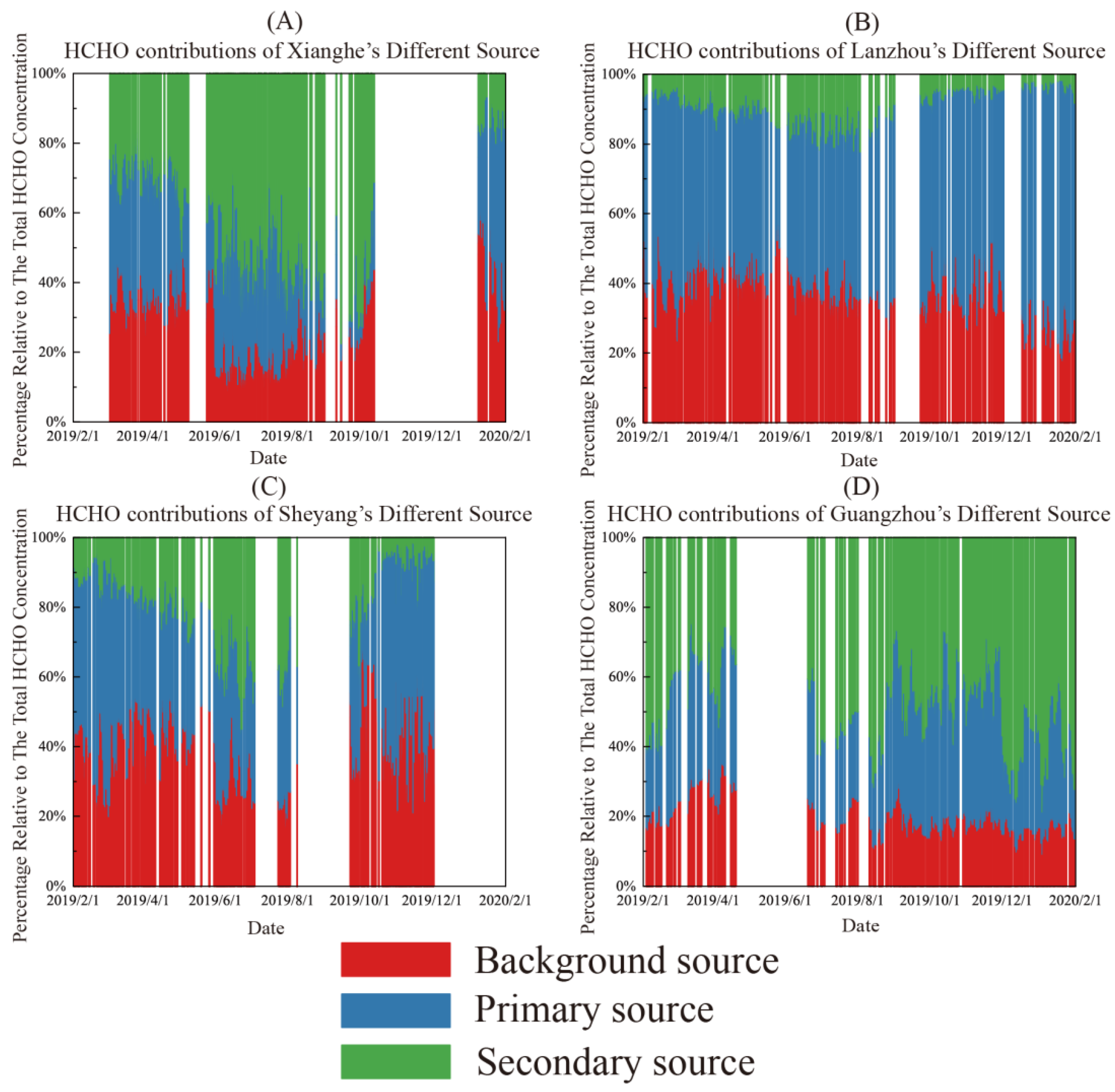
4.1. Primary and Secondary Sources of HCHO in Four Cities

In this section, we use data from the CNEMC sites and the near-surface results from the MAX-DOAS profiles to distinguish the contributions of the primary, secondary, and background sources of HCHO in the lower atmosphere in the four cities.

In previous studies, the background value was often fixed at 1 ppbv [44,68]. Therefore, we set the background source as a constant value of 1 and calculated primary and secondary formaldehyde for the four regions based on the methodology outlined in Section 2.4. We compared the fitted HCHO results with the measured HCHO, and Figure 7A–P presents the results. In Figure 7A–P, the slopes and intercepts of all simulation results are consistently set to 1. From Figure 7A–P, it can be observed that only the simulation results for spring in Shenyang (Figure 7I) exhibit a correlation of 0.857. This indicates a strong correlation between the simulated and actual HCHO concentrations. However, in seasons other than spring in Shenyang and in all seasons in the other cities, the overall correlation coefficients range approximately between 0.3 and 0.8. This implies a relatively weaker correlation between the simulated HCHO concentrations and the actual HCHO concentrations.

Figure 8A shows the annual contributions of HCHO in Xianghe. During summer and autumn, the major contributions of HCHO are from secondary sources, accounting for 54.32% (±14.26%) and 62.20% (±15.08%) of the total HCHO sources, respectively. However, in spring, the primary, secondary, and background sources show significant contributions, accounting for 34.09% (±13.08%), 30.80% (±9.75%), and 35.12% (±6.73%) of the total sources, respectively. During winter, primary and background sources dominate, contributing 40.00% ± 15.57% and 44.87% ± 11.81% of the total HCHO sources, respectively. This indicates that in Xianghe, an eastern city, HCHO primarily arises from volatile organic compound emissions during summer and autumn. However, in the seasons with less sunlight, such as spring and winter, the process of converting volatile organic compounds into HCHO is somewhat inhibited, while heating combustion increases the contribution from primary sources.

Figure 8B shows the annual contributions of HCHO in Lanzhou. In Lanzhou, throughout the year, primary sources dominate HCHO emissions, contributing 49.16% (±11.09%), 48.26% (±10.31%), 56.29% (±10.13%), and 61.45% (±12.80%) in spring, summer, autumn, and winter, respectively. These results show that, in Lanzhou, a developing city in the west, HCHO mainly stems from initial atmospheric pollutants, biomass combustion, and industrial emissions.

Figure 8C shows the annual contributions of HCHO in Shenyang. The trend in the HCHO contribution in Shenyang exhibits some similarities to that in Xianghe, where the contribution from primary sources significantly increases during spring and winter, while it decreases, to some extent, during summer and autumn. However, as Shenyang is relatively more northern than Xianghe, it experiences more industrial emissions and biomass burning. Hence, primary sources dominate during spring and winter, at 41.20% (±14.02%) and 51.06% (±13.52%), respectively. In contrast, both primary and secondary sources contribute significantly to the HCHO concentrations during summer and autumn in Shenyang.

Figure 8D shows the annual contributions of HCHO in Guangzhou. Throughout the year in Guangzhou, HCHO is predominantly derived from secondary sources, accounting for 38.01% (±11.41%), 55.49% (±13.79%), 69.05% (±12.13%), and 60.15% (±11.35%) during the four seasons. Given Guangzhou’s status as a developed city with significant vehicular traffic and substantial emissions of methane and non-methane hydrocarbons, coupled with the favorable sunlight conditions year-round, the generation of secondary HCHO is intensified.

Based on the analysis above, there are significant variations in HCHO emissions among the four cities. In the humid eastern city of Xianghe, volatile organic compounds predominantly contribute to HCHO emissions during summer and autumn, while primary and background sources become more prominent in spring and winter due to reduced sunlight and increased heating combustion. In Lanzhou, a developing western city, primary sources consistently dominate HCHO emissions throughout the year, originating from atmospheric pollutants, biomass combustion, and industrial emissions. Shenyang exhibits similar seasonal trends to Xianghe, but being further north, has higher industrial emissions and biomass burning, leading to primary sources dominating in spring and winter. In Guangzhou, a developed city with substantial vehicular traffic and year-round favorable sunlight, secondary sources intensify, contributing significantly to HCHO concentrations throughout the year.

4.2. O₃-NO_x-VOCs Sensitivities in Vertical Space in Four Cities

Finally, we analyzed the near-surface O₃ sensitivities in the four cities. The O₃ sensitivity is mainly determined by the ratio of HCHO/NO₂. Based on the CNEMC observation data of O₃ and the near-surface vertical profiles retrieved by precursors in the four cities in the different seasons, the near-surface O₃ sensitivities in different seasons can be calculated. These results can better aid in O₃ monitoring and prevention in different industrial parks in China.

Due to the significant variations in O₃ across the different regions and seasons, it is necessary to employ the above algorithm to systematically screen, calculate, and determine the thresholds for each city in different seasons. This helps to analyze the O₃ sensitivity of the four cities across various seasons. Here, we utilized the measured O₃ concentration data from the CNEMC station nearest to the MAX-DOAS sites, the measured NO₂ concentration data from the MAX-DOAS sites, and the secondary HCHO data obtained through simulation analysis in Section 4.1. We calculated the sensitivity thresholds for O₃ in different seasons and locations using the methodology outlined in Section 2.5. Figure 9 illustrates the O₃ sensitivity for the four cities across the four seasons. In Figure 9, the light- pink background indicates that O₃ generation is considered to be VOC limited, the light-yellow background indicates that O₃ generation is considered to be transitional between VOCs and NO_x, and the light-gray background indicates that O₃ generation is considered to be NO_x limited.

Table 3. The specific parameters of O₃ sensitivity in different seasons for the four cities.

City	Season	Threshold	VOCs	NOx-VOCs	NOx
Xianghe	Spring	[0.2, 0.5]	71.76%	22.90%	5.34%
	Summer	[0.8, 1.8]	44.83%	36.38%	18.78%
	Autumn	[0.5, 0.9]	50.53%	22.11%	27.34%
	Winter	[0.07, 0.1]	71.03%	12.15%	16.82%
Lanzhou	Spring	[0.045, 0.080]	69.39%	25.07%	5.54%
	Summer	[0.09, 0.12]	54.82%	18.94%	26.25%
	Autumn	[0.007, 0.008]	11.96%	7.18%	80.86%
	Winter	[0.014, 0.021]	73.36%	21.83%	4.80%
Shenyang	Spring	[0.042, 0.065]	38.30%	30.70%	31.00%
	Summer	[0.15, 0.23]	37.04%	22.75%	40.21%
	Autumn	[0.04, 0.14]	51.76%	44.72%	3.52%
	Winter	[0.016, 0.023]	24.04%	17.31%	58.66%
Guangzhou	Spring	[0.19, 0.31]	82.22%	12.22%	5.56%
	Summer	[0.34, 0.47]	35.48%	19.35%	45.16%
	Autumn	[0.3, 0.6]	53.79%	31.05%	15.16%
	Winter	[0.19, 0.35]	33.48%	33.03%	33.48%

provides more detailed O₃ sensitivity parameters for the four cities. In Xianghe, during spring, autumn, and winter, the near-surface O₃ sensitivity is primarily influenced by VOC-limited conditions, accounting for 71.76%, 50.53%, and 71.03%, respectively. However, in summer, the near-surface O₃ sensitivity is mainly affected by VOC-limited conditions and is transitional between VOCs and NO_x, accounting for 44.83% and 36.38%, respectively, while NO_x-limited conditions remain minimal across all four seasons.

In Lanzhou, during spring, summer, and winter of the same year, the near-surface O₃ sensitivity was primarily influenced by VOC-limited conditions, accounting for 69.39%, 52.82%, and 73.36%, respectively. However, during autumn, the near-surface O₃ sensitivity was predominantly affected by NO_x-limited conditions, accounting for nearly 80.86%.

In Shenyang, during spring and summer, the near-surface O₃ sensitivity is primarily influenced by a combination of VOC-limited conditions, transitional interference, and NO_x-limited conditions. During autumn, the near-surface O₃ sensitivity is mainly affected by VOC-limited conditions, accounting for 51.76%. However, during winter, the near-surface O₃ sensitivity is primarily influenced by NO_x-limited conditions, accounting for 58.66%.

In the Guangzhou area, during spring and autumn, the near-surface O₃ sensitivity is mainly affected by VOC-limited conditions, accounting for 82.22% and 53.79%, respectively. In summer, the influence is mainly derived from both VOC-limited and NO_x-limited conditions, accounting for 35.48% and 45.16% of the total interference time, respectively. During winter in Guangzhou, the near-surface O₃ sensitivity is more evenly affected by VOC-limited conditions, NO_x-limited conditions, and transitional interference between VOCs and NO_x.

According to the Technical Regulation on Ambient Air Quality Index (AQI) of China, O₃ concentrations exceeding 160 μg/m³ per hour are classified as O₃ pollution. In some parts of Figure 9A–P, there is a green dashed line. O₃ data points above this green dashed line in the figure represent O₃ pollution in this area during this specific time period. From Figure 9, it is evident that there are extended periods of O₃ pollution during summer (Figure 9B,F,J,N) across all four regions as well as during autumn in Guangzhou and Xianghe (Figure 9C,O). Figure S3 in the Supplementary Materials illustrates the time periods during which O₃ pollution was monitored at these sites. Therefore, we conducted a more detailed analysis of these six extended pollution periods.

As shown in Figure 9B, from 1 June 2019 to 31 August 2019, in Xianghe, approximately 24.53% of the time period was marked by O₃ pollution as per the MAX-DOAS instrument records. Within these O₃-polluted periods, the O₃ sensitivity was predominantly affected. Approximately 39.31% of the time, the region experienced transitional interference between VOCs and NO_x, while 60% of the time, it was primarily influenced by NO_x-limited conditions. Despite Xianghe’s summer being largely influenced by VOC-limited conditions and transitional interference between VOCs and NO_x, the presence of NO_x-limited conditions led to a higher level of O₃ pollution. As seen in Figure 9C and Figure S3, Xianghe experienced significant O₃ pollution during the afternoon period from 22 September 2019 to 3 October 2019. Throughout this period, Xianghe’s O₃ sensitivity was predominantly influenced by NO_x-limited conditions. Therefore, it can be concluded that the autumn O₃ pollution in Xianghe primarily stemmed from NO_x-limited conditions.

Lanzhou experiences relatively low O₃ pollution throughout the year. However, in Figure 9F and Figure S3, instances of O₃ pollution in the afternoon period can be observed from 12 July 2019 to 12 August 2019, a month-long timespan. During these times, the O₃ sensitivity in Lanzhou was also predominantly influenced by NO_x-limited conditions. This indicates that NO_x-limited situations, similarly, constitute the primary cause of O₃ pollution in the Lanzhou region during these periods.

In the Shenyang region, the occurrence of O₃ pollution is relatively high compared to Lanzhou, although it still predominantly occurs during the summer. As shown in Figure 9J, during the two observation periods—2 June 2019 to June 12, 2019, and July 26, 2019, to 1 August 2019—Shenyang experienced notable O₃ pollution near the surface. Similarly, during these O₃-polluted times, the O₃ sensitivity was primarily within the NO_x-limited range. Hence, it is evident that NO_x-limited conditions also serve as the main cause of O₃ pollution in the Shenyang region.

In the Guangzhou region, O₃ pollution was mainly concentrated during the afternoon from 11 August to 22 August in 2019 (as depicted in Figure 9N and Figure S3) and during the afternoon from 8 September to 27 November in 2019 (as illustrated in Figure 9O). In the near-ground O₃ pollution periods in Guangzhou’s summer, the primary influence was NO_x limited. However, during the near-ground pollution periods in Guangzhou’s autumn, the O₃ sensitivity indicates that 39.17% of the time period was mainly influenced by a transitional interference between VOCs and NO_x interference, while another 48.45% of the time period was primarily affected by NO_x limitations. As indicated in Table 3, Guangzhou is expected to be predominantly VOC limited in autumn. Nonetheless, transitional interference and NO_x limitations resulted in more O₃ pollution periods during this time.

Based on the analysis above, although the O₃ sensitivity was found in different seasons in the four cities, the main cause of O₃ exceeding the threshold is NO_x limited. Therefore, anthropogenic emissions of NO_x are the primary cause of O₃ pollution in the four cities mentioned above.

5. Conclusions

The study used ground-based MAX-DOAS instruments to analyze the seasonal variations of two pollutants, NO₂ and HCHO, in typical cities across the eastern, western, northern, and southern regions of China. Spectral data collected by MAX-DOAS from February 2019 to January 2020 were used to retrieve the vertical profiles of NO₂ and HCHO in these four cities. A comparison between the near-surface NO₂ concentrations obtained from the vertical profiles and the CNEMC in situ of each site’s NO₂ results exhibited high consistency between the two datasets.

We first analyzed the variations in the NO₂ and HCHO concentrations across the four cities. The cities exhibited varied NO₂ and HCHO concentrations across the seasons. Xianghe consistently recorded the lowest NO₂ values, indicating lower emissions than the other cities. Guangzhou, with its advanced economy and vehicle ownership, showed higher NO₂ and HCHO concentrations in spring. Summer brought elevated HCHO concentrations in Guangzhou, Xianghe, and Shenyang due to the intensified photochemical processes, contrasting with the lower values in Lanzhou. Autumn and winter showed a similar evolution, highlighting higher HCHO concentrations in Guangzhou and Xianghe compared to Lanzhou and Shenyang. Overall, Guangzhou exhibited the highest annual average concentrations of NO₂ and HCHO due to its developed economy and industrial emissions. Xianghe’s lower NO₂ values may result from reduced industrial and vehicular emissions, offset by higher O₃ values, leading to elevated HCHO concentrations.

Next, we analyzed the near-surface primary and secondary sources of HCHO across different seasons in each city based on the near-surface CO and O₃ data provided by the CNEMC sites. The HCHO source analysis across the four cities reveals distinctive patterns: in Xianghe, secondary sources dominate during summer and autumn, while primary, secondary, and background sources contribute significantly in spring and winter. In Lanzhou, the primary source dominates the HCHO concentrations in spring, summer, autumn, and winter, amounting to approximately 49.16%, 48.26%, 56.29%, and 61.45%, respectively. This distinct seasonal variation in HCHO sources emphasizes the influence of natural and anthropogenic factors on HCHO generation, reflecting the city’s characteristics as a developing western region with specific pollution origins. Shenyang’s seasonal trend contributions of HCHO show similarities to Xianghe due to industrial emissions and biomass burning. In Guangzhou, a developed city, HCHO is predominantly derived from secondary sources, accounting for 38.01%, 55.49%, 69.05%, and 60.15% during the four seasons, correlating with its high levels of vehicular traffic and favorable sunlight conditions. These findings reveal the seasonal dynamics of HCHO sources, showing the interplay between primary and secondary emissions in different urban contexts.

Finally, we analyzed the differences in O₃ sensitivity across different seasons in the four cities based on the near-surface HCHO and NO₂ results obtained from MAX-DOAS. The four cities again exhibited distinct seasonal variations. In these four cities, the influence of VOCs and NO_x on the near-surface O₃ sensitivity varies across different seasons. In Xianghe, VOCs predominantly impact the O₃ levels during spring, autumn, and winter, accounting for 71.76%, 50.53%, and 71.03%, respectively. However, in summer, both VOCs and NO_x significantly affect O₃, contributing 44.83% and 36.38%, respectively. Lanzhou experiences VOC-driven O₃ sensitivity in spring, summer, and winter, at 69.39%, 52.82%, and 73.36%, respectively, while autumn is primarily influenced by NO_x, reaching 80.86%. In Shenyang, VOCs, transitional interference, and NO_x collectively affect O₃ sensitivity in spring and summer, whereas autumn is primarily impacted by VOCs (51.76%), and winter is predominantly influenced by NO_x (58.66%). In Guangzhou, VOCs have a substantial impact during spring (82.22%) and autumn (53.79%), while in summer, both VOCs (35.48%) and NO_x (45.16%) play significant roles. Winter in Guangzhou demonstrates a more balanced influence from VOCs, NO_x, and their transition. The primary near-ground O₃ pollution periods in the four regions of China are concentrated during the afternoon hours of the summer season, and their O₃ sensitivity is predominantly influenced by NO_x-limited conditions.

Based on the above results, Xianghe and other eastern cities in China need to pay more attention to the precursors of secondary sources of formaldehyde during summer and autumn. Lanzhou and other western cities in China may need to focus on the heavy industrial combustion emissions of primary formaldehyde throughout the year. For Shenyang and other northern cities in China, heavy industrial combustion emissions in winter and spring are more likely to increase primary formaldehyde, causing excessive levels. Meanwhile, Guangzhou and other southern cities in China need to be vigilant about the precursors of secondary sources of formaldehyde throughout the year. On the other hand, all cities nationwide need to control anthropogenic emissions of NO as these emissions are more likely to cause urban O₃ pollution.

References

1. Li, G.; Fang, C.; Sun, S. The effect of economic growth, urbanization, and industrialization on fine particulate matter (PM2.5) concentrations in China. Environ. Sci. Technol. 2016, 50, 11452–11459. [Google Scholar] [CrossRef]
2. Zhang, Z.; Zhang, X.; Gong, D.; Quan, W.; Zhao, X.; Ma, Z.; Kim, S.-J. Evolution of surface O3 and PM2.5 concentrations and their relationships with meteorological conditions over the last decade in Beijing. Atmos. Environ. 2015, 108, 67–75. [Google Scholar] [CrossRef]
3. Knowlton, K.; Rosenthal, J.E.; Hogrefe, C.; Lynn, B.; Gaffin, S.; Goldberg, R.; Rosenzweig, C.; Civerolo, K.; Ku, J.-Y.; Kinney, P.L. Assessing ozone-related health impacts under a changing climate. Environ. Health Perspect. 2004, 112, 1557–1563. [Google Scholar] [CrossRef]
4. Li, Y.; Yin, S.; Yu, S.; Bai, L.; Wang, X.; Lu, X.; Ma, S. Characteristics of ozone pollution and the sensitivity to precursors during early summer in central plain, China. J. Environ. Sci. 2021, 99, 354–368. [Google Scholar] [CrossRef]
5. Kgabi, N.A.; Sehloho, R.M. Seasonal variations of tropospheric ozone concentrations. Glob. J. Sci. Front. Res. 2012, 12, 21–29. [Google Scholar]
6. Zhang, Z.; Yao, M.; Wu, W.; Zhao, X.; Zhang, J. Spatiotemporal assessment of health burden and economic losses attributable to short-term exposure to ground-level ozone during 2015–2018 in China. BMC Public Health 2021, 21, 1069. [Google Scholar] [CrossRef]
7. Ren, B.; Xie, P.; Xu, J.; Li, A.; Qin, M.; Hu, R.; Zhang, T.; Fan, G.; Tian, X.; Zhu, W.; et al. Vertical characteristics of NO2 and HCHO, and the ozone formation regimes in Hefei, China. Sci. Total Environ. 2022, 823, 153425. [Google Scholar] [CrossRef] [PubMed]
8. Steiner, A.L.; Cohen, R.C.; Harley, R.A.; Tonse, S.; Millet, D.B.; Schade, G.W.; Goldstein, A.H. VOC reactivity in central California: Comparing an air quality model to ground-based measurements. Atmos. Chem. Phys. 2008, 8, 351–368. [Google Scholar] [CrossRef]
9. Mohajan, H. Acid rain is a local environment pollution but global concern. Open Sci. J. Anal. Chem. 2018, 3, 47–55. [Google Scholar]
10. Altshuller, A.P. Production of aldehydes as primary emissions and from secondary atmospheric reactions of alkenes and alkanes during the night and early morning hours. Atmos. Environ. Part A General. Top. 1993, 27, 21–32. [Google Scholar] [CrossRef]
11. Levy, H. Normal atmosphere: Large radical and formaldehyde concentrations predicted. Science 1971, 173, 141–143. [Google Scholar] [CrossRef]
12. Parrish, D.D.; Ryerson, T.B.; Mellqvist, J.; Johansson, J.; Fried, A.; Richter, D.; Walega, J.G.; Washenfelder, R.A.; de Gouw, J.A.; Peischl, J.; et al. Primary and secondary sources of formaldehyde in urban atmospheres: Houston Texas region. Atmos. Chem. Phys. 2012, 12, 3273–3288. [Google Scholar] [CrossRef]
13. Rappenglück, B.; Dasgupta, P.K.; Leuchner, M.; Li, Q.; Luke, W. Formaldehyde and its relation to CO, PAN, and SO2 in the Houston-Galveston airshed. Atmos. Chem. Phys. 2010, 10, 2413–2424. [Google Scholar] [CrossRef]
14. Carter, W.P.L. Development of ozone reactivity scales for volatile organic compounds. Air Waste 1994, 44, 881–899. [Google Scholar] [CrossRef]
15. De Smedt, I.; Müller, J.F.; Stavrakou, T.; van der A, R.; Eskes, H.; Van Roozendael, M. Twelve years of global observations of formaldehyde in the troposphere using GOME and SCIAMACHY sensors. Atmos. Chem. Phys. 2008, 8, 4947–4963. [Google Scholar] [CrossRef]
16. Ma, Y.; Diao, Y.; Zhang, B.; Wang, W.; Ren, X.; Yang, D.; Wang, M.; Shi, X.; Zheng, J. Detection of formaldehyde emissions from an industrial zone in the Yangtze River Delta region of China using a proton transfer reaction ion-drift chemical ionization mass spectrometer. Atmos. Meas. Tech. 2016, 9, 6101–6116. [Google Scholar] [CrossRef]
17. Friedfeld, S.; Fraser, M.; Ensor, K.; Tribble, S.; Rehle, D.; Leleux, D.; Tittel, F. Statistical analysis of primary and secondary atmospheric formaldehyde. Atmos. Environ. 2002, 36, 4767–4775. [Google Scholar] [CrossRef]
18. Wood, E.C.; Canagaratna, M.R.; Herndon, S.C.; Onasch, T.B.; Kolb, C.E.; Worsnop, D.R.; Kroll, J.H.; Knighton, W.B.; Seila, R.; Zavala, M.; et al. Investigation of the correlation between odd oxygen and secondary organic aerosol in Mexico City and Houston. Atmos. Chem. Phys. 2010, 10, 8947–8968. [Google Scholar] [CrossRef]
19. Li, Y.; Shao, M.; Lu, S.; Chang, C.-C.; Dasgupta, P.K. Variations and sources of ambient formaldehyde for the 2008 Beijing Olympic games. Atmos. Environ. 2010, 44, 2632–2639. [Google Scholar] [CrossRef]
20. Lui, K.H.; Ho, S.S.H.; Louie, P.K.K.; Chan, C.S.; Lee, S.C.; Hu, D.; Chan, P.W.; Lee, J.C.W.; Ho, K.F. Seasonal behavior of carbonyls and source characterization of formaldehyde (HCHO) in ambient air. Atmos. Environ. 2017, 152, 51–60. [Google Scholar] [CrossRef]
21. Garcia, A.R.; Volkamer, R.; Molina, L.T.; Molina, M.J.; Samuelson, J.; Mellqvist, J.; Galle, B.; Herndon, S.C.; Kolb, C.E. Separation of emitted and photochemical formaldehyde in Mexico City using a statistical analysis and a new pair of gas-phase tracers. Atmos. Chem. Phys. 2006, 6, 4545–4557. [Google Scholar] [CrossRef]
22. Kong, L.; Tang, X.; Zhu, J.; Wang, Z.; Li, J.; Wu, H.; Wu, Q.; Chen, H.; Zhu, L.; Wang, W.; et al. A 6-year-long (2013–2018) high-resolution air quality reanalysis dataset in China based on the assimilation of surface observations from CNEMC. Earth Syst. Sci. Data 2021, 13, 529–570. [Google Scholar] [CrossRef]
23. Hönninger, G.; Von Friedeburg, C.; Platt, U. Multi axis differential optical absorption spectroscopy (MAX-DOAS). Atmos. Chem. Phys. 2004, 4, 231–254. [Google Scholar] [CrossRef]
24. Irie, H.; Takashima, H.; Kanaya, Y.; Boersma, K.F.; Gast, L.; Wittrock, F.; Brunner, D.; Zhou, Y.; Van Roozendael, M. Eight-component retrievals from ground-based MAX-DOAS observations. Atmos. Meas. Tech. 2011, 4, 1027–1044. [Google Scholar] [CrossRef]
25. Liu, C.; Xing, C.; Hu, Q.; Li, Q.; Liu, H.; Hong, Q.; Tan, W.; Ji, X.; Lin, H.; Lu, C.; et al. Ground-based hyperspectral stereoscopic remote sensing network: A promising strategy to learn coordinated control of O3 and PM2.5 over China. Engineering 2022, 19, 71–83. [Google Scholar] [CrossRef]
26. Lampel, J.; Pöhler, D.; Horbanski, M.; Platt, U. Performance of Airyx SkySpec MAX-DOAS systems during different field campaigns. Geophys. Res. Abstr. 2019, 21, 12267. [Google Scholar]
27. Stutz, J.; Platt, U. Numerical analysis and estimation of the statistical error of differential optical absorption spectroscopy measurements with least-squares methods. Appl. Opt. 1996, 35, 6041–6053. [Google Scholar] [CrossRef] [PubMed]
28. Danckaert, T.; Fayt, C.; Van Roozendael, M. QDOAS Software User Manual. 2012. Available online: https://uv-vis.aeronomie.be/software/QDOAS/ (accessed on 1 January 2024).
29. Chance, K.; Kurucz, R.L. An improved high-resolution solar reference spectrum for earth’s atmosphere measurements in the ultraviolet, visible, and near infrared. J. Quant. Spectrosc. Radiat. Transf. 2010, 111, 1289–1295. [Google Scholar] [CrossRef]
30. Keller-Rudek, H.; Moortgat, G.K.; Sander, R.; Sörensen, R. The MPI-Mainz UV/VIS Spectral Atlas of Gaseous Molecules of Atmospheric Interest. Earth Syst. Sci. Data. 2013, 5, 365–373. [Google Scholar] [CrossRef]
31. Rozanov, V.V.; Buchwitz, M.; Eichmann, K.U.; de Beek, R.; Burrows, J.P. SCIATRAN—A new radiative transfer model for geophysical applications in the 240–2400 nm spectral region: The pseudo-spherical version. Adv. Space Res. 2002, 29, 1831–1835. [Google Scholar] [CrossRef]
32. Vandaele, A.C.; Hermans, C.; Simon, P.C.; Carleer, M.; Colin, R.; Fally, S.; Mérienne, M.F.; Jenouvrier, A.; Coquart, B. Measurements of the NO2 absorption cross-section from 42,000 cm−1 to 10,000 cm−1 (238–1000 nm) at 220 K and 294 K. J. Quant. Spectrosc. Radiat. Transf. 1998, 59, 171–184. [Google Scholar] [CrossRef]
33. Serdyuchenko, A.; Gorshelev, V.; Weber, M.; Chehade, W.; Burrows, J.P. High spectral resolution ozone absorption cross-sections—Part 2: Temperature dependence. Atmos. Meas. Tech. 2014, 7, 625–636. [Google Scholar] [CrossRef]
34. Volkamer, R.; Spietz, P.; Burrows, J.; Platt, U. High-resolution absorption cross-section of glyoxal in the UV–vis and IR spectral ranges. J. Photochem. Photobiol. A Chem. 2005, 172, 35–46. [Google Scholar] [CrossRef]
35. Fleischmann, O.C.; Hartmann, M.; Burrows, J.P.; Orphal, J. New ultraviolet absorption cross-sections of BrO at atmospheric temperatures measured by time-windowing Fourier transform spectroscopy. J. Photochem. Photobiol. A Chem. 2004, 168, 117–132. [Google Scholar] [CrossRef]
36. Meller, R.; Moortgat, G.K. Temperature dependence of the absorption cross sections of formaldehyde between 223 and 323 K in the wavelength range 225–375 nm. J. Geophys. Res. Atmos. 2000, 105, 7089–7101. [Google Scholar] [CrossRef]
37. Chance, K.V.; Spurr, R.J.D. Ring effect studies: Rayleigh scattering, including molecular parameters for rotational Raman scattering, and the Fraunhofer spectrum. Appl. Opt. 1997, 36, 5224–5230. [Google Scholar] [CrossRef] [PubMed]
38. Chan, K.L.; Wiegner, M.; van Geffen, J.; De Smedt, I.; Alberti, C.; Cheng, Z.; Ye, S.; Wenig, M. MAX-DOAS measurements of tropospheric NO2 and HCHO in Munich and the comparison to OMI and TROPOMI satellite observations. Atmos. Meas. Tech. 2020, 13, 4499–4520. [Google Scholar] [CrossRef]
39. Chan, K.L.; Wiegner, M.; Wenig, M.; Pöhler, D. Observations of tropospheric aerosols and NO2 in Hong Kong over 5 years using ground based MAX-DOAS. Sci. Total Environ. 2018, 619–620, 1545–1556. [Google Scholar] [CrossRef] [PubMed]
40. Rodgers, C.D. Inverse Methods for Atmospheric Sounding: Theory and Practice; World Scientific: Singapore, 2000. [Google Scholar]
41. Wagner, T.; Dix, B.; Friedeburg, C.v.; Frieß, U.; Sanghavi, S.; Sinreich, R.; Platt, U. MAX-DOAS O4 measurements: A new technique to derive information on atmospheric aerosols—Principles and information content. J. Geophys. Res. Atmos. 2004, 109, D22205. [Google Scholar] [CrossRef]
42. Seyler, A.; Wittrock, F.; Kattner, L.; Mathieu-Üffing, B.; Peters, E.; Richter, A.; Schmolke, S.; Burrows, J.P. Monitoring shipping emissions in the German Bight using MAX-DOAS measurements. Atmos. Chem. Phys. 2017, 17, 10997–11023. [Google Scholar] [CrossRef]
43. Lin, H.; Xing, C.; Hong, Q.; Liu, C.; Ji, X.; Liu, T.; Lin, J.; Lu, C.; Tan, W.; Li, Q.; et al. Diagnosis of Ozone Formation Sensitivities in Different Height Layers via MAX-DOAS Observations in Guangzhou. J. Geophys. Res. Atmos. 2022, 127, e2022JD036803. [Google Scholar] [CrossRef]
44. Hong, Q.; Liu, C.; Chan, K.L.; Hu, Q.; Xie, Z.; Liu, H.; Si, F.; Liu, J. Ship-based MAX-DOAS measurements of tropospheric NO2, SO2, and HCHO distribution along the Yangtze River. Atmos. Chem. Phys. 2018, 18, 5931–5951. [Google Scholar] [CrossRef]
45. Sun, Y.; Yin, H.; Liu, C.; Zhang, L.; Cheng, Y.; Palm, M.; Notholt, J.; Lu, X.; Vigouroux, C.; Zheng, B.; et al. Mapping the drivers of formaldehyde (HCHO) variability from 2015 to 2019 over eastern China: Insights from Fourier transform infrared observation and GEOS-Chem model simulation. Atmos. Chem. Phys. 2021, 21, 6365–6387. [Google Scholar] [CrossRef]
46. Su, W.J.; Liu, C.; Hu, Q.H.; Zhao, S.H.; Sun, Y.W.; Wang, W.; Zhu, Y.Z.; Liu, J.G.; Kim, J. Primary and secondary sources of ambient formaldehyde in the Yangtze River Delta based on Ozone Mapping and Profiler Suite (OMPS) observations. Atmos. Chem. Phys. 2019, 19, 6717–6736. [Google Scholar] [CrossRef]
47. Souri, A.H.; Nowlan, C.R.; Wolfe, G.M.; Lamsal, L.N.; Chan Miller, C.E.; Abad, G.G.; Janz, S.J.; Fried, A.; Blake, D.R.; Weinheimer, A.J.; et al. Revisiting the effectiveness of HCHO/NO2 ratios for inferring ozone sensitivity to its precursors using high resolution airborne remote sensing observations in a high ozone episode during the KORUS-AQ campaign. Atmos. Environ. 2020, 224, 117341. [Google Scholar] [CrossRef]
48. Chen, X.; Zhan, J.; Su, W. Analyses of velocity field and energy transmission in the interaction between adjacent twin floating bodies and waves. Prog. Comput. Fluid Dyn. Int. J. 2017, 17, 221–231. [Google Scholar] [CrossRef]
49. Vallecillos, L.; Marcé, R.M.; Borrull, F. Applicability of a gas chromatograph-photoionization detection analyzer for the continuous monitoring of 1,3-butadiene in urban and industrial atmospheres. Atmos. Pollut. Res. 2024, 15, 101949. [Google Scholar] [CrossRef]
50. Tang, Z.; Guo, J.; Zhou, J.; Yu, H.; Wang, Y.; Lian, X.; Ye, J.; He, X.; Han, R.; Li, J.; et al. The impact of short-term exposures to ambient NO2, O3, and their combined oxidative potential on daily mortality. Environ. Res. 2024, 241, 117634. [Google Scholar] [CrossRef]
51. Kumar, V.; Beirle, S.; Dörner, S.; Mishra, A.K.; Donner, S.; Wang, Y.; Sinha, V.; Wagner, T. Long-term MAX-DOAS measurements of NO2, HCHO, and aerosols and evaluation of corresponding satellite data products over Mohali in the Indo-Gangetic Plain. Atmos. Chem. Phys. 2020, 20, 14183–14235. [Google Scholar] [CrossRef]
52. Xue, J.; Zhao, T.; Luo, Y.; Miao, C.; Su, P.; Liu, F.; Zhang, G.; Qin, S.; Song, Y.; Bu, N.; et al. Identification of ozone sensitivity for NO2 and secondary HCHO based on MAX-DOAS measurements in northeast China. Environ. Int. 2022, 160, 107048. [Google Scholar] [CrossRef]
53. Tirpitz, J.L.; Frieß, U.; Spurr, R.; Platt, U. Enhancing MAX-DOAS atmospheric state retrievals by multispectral polarimetry—Studies using synthetic data. Atmos. Meas. Tech. 2022, 15, 2077–2098. [Google Scholar] [CrossRef]
54. Tian, X.; Chen, M.; Xie, P.; Xu, J.; Li, A.; Ren, B.; Zhang, T.; Fan, G.; Wang, Z.; Zheng, J.; et al. Evaluation of MAX-DOAS Profile Retrievals under Different Vertical Resolutions of Aerosol and NO2 Profiles and Elevation Angles. Remote Sens. 2023, 15, 5431. [Google Scholar] [CrossRef]
55. Bösch, T.; Rozanov, V.; Richter, A.; Peters, E.; Rozanov, A.; Wittrock, F.; Merlaud, A.; Lampel, J.; Schmitt, S.; de Haij, M.; et al. BOREAS—A new MAX-DOAS profile retrieval algorithm for aerosols and trace gases. Atmos. Meas. Tech. 2018, 11, 6833–6859. [Google Scholar] [CrossRef]
56. Wang, Y.; Dörner, S.; Donner, S.; Böhnke, S.; De Smedt, I.; Dickerson, R.R.; Dong, Z.; He, H.; Li, Z.; Li, Z.; et al. Vertical profiles of NO2, SO2, HONO, HCHO, CHOCHO and aerosols derived from MAX-DOAS measurements at a rural site in the central western North China Plain and their relation to emission sources and effects of regional transport. Atmos. Chem. Phys. 2019, 19, 5417–5449. [Google Scholar] [CrossRef]
57. Hong, Q.; Liu, C.; Hu, Q.; Xing, C.; Tan, W.; Liu, H.; Huang, Y.; Zhu, Y.; Zhang, J.; Geng, T.; et al. Evolution of the vertical structure of air pollutants during winter heavy pollution episodes: The role of regional transport and potential sources. Atmos. Res. 2019, 228, 206–222. [Google Scholar] [CrossRef]
58. Miao, Y.; Guo, J.; Liu, S.; Liu, H.; Li, Z.; Zhang, W.; Zhai, P. Classification of summertime synoptic patterns in Beijing and their associations with boundary layer structure affecting aerosol pollution. Atmos. Chem. Phys. 2017, 17, 3097–3110. [Google Scholar] [CrossRef]
59. Sun, Z.; Zhao, X.; Li, Z.; Tang, G.; Miao, S. Boundary layer structure characteristics under objective classification of persistent pollution weather types in the Beijing area. Atmos. Chem. Phys. 2021, 21, 8863–8882. [Google Scholar] [CrossRef]
60. Xu, T.; Song, Y.; Liu, M.; Cai, X.; Zhang, H.; Guo, J.; Zhu, T. Temperature inversions in severe polluted days derived from radiosonde data in North China from 2011 to 2016. Sci. Total Environ. 2019, 647, 1011–1020. [Google Scholar] [CrossRef]
61. Atkinson, R.; Arey, J. Gas-phase tropospheric chemistry of biogenic volatile organic compounds: A review. Atmos. Environ. 2003, 37, 197–219. [Google Scholar] [CrossRef]
62. Luecken, D.J.; Hutzell, W.T.; Strum, M.L.; Pouliot, G.A. Regional sources of atmospheric formaldehyde and acetaldehyde, and implications for atmospheric modeling. Atmos. Environ. 2012, 47, 477–490. [Google Scholar] [CrossRef]
63. Wu, Y.; Huo, J.; Yang, G.; Wang, Y.; Wang, L.; Wu, S.; Yao, L.; Fu, Q.; Wang, L. Measurement report: Production and loss of atmospheric formaldehyde at a suburban site of Shanghai in summertime. Atmos. Chem. Phys. 2023, 23, 2997–3014. [Google Scholar] [CrossRef]
64. Ma, T.; Furutani, H.; Duan, F.; Kimoto, T.; Jiang, J.; Zhang, Q.; Xu, X.; Wang, Y.; Gao, J.; Geng, G.; et al. Contribution of hydroxymethanesulfonate (HMS) to severe winter haze in the North China Plain. Atmos. Chem. Phys. 2020, 20, 5887–5897. [Google Scholar] [CrossRef]
65. Moch, J.M.; Dovrou, E.; Mickley, L.J.; Keutsch, F.N.; Cheng, Y.; Jacob, D.J.; Jiang, J.; Li, M.; Munger, J.W.; Qiao, X.; et al. Contribution of hydroxymethane sulfonate to ambient particulate matter: A potential explanation for high particulate sulfur during severe winter haze in Beijing. Geophys. Res. Lett. 2018, 45, 11969–11979. [Google Scholar] [CrossRef]
66. Shen, Y.; Jiang, F.; Feng, S.; Zheng, Y.; Cai, Z.; Lyu, X. Impact of weather and emission changes on NO2 concentrations in China during 2014–2019. Environ. Pollut. 2021, 269, 116163. [Google Scholar] [CrossRef]
67. Li, X.; Brauers, T.; Hofzumahaus, A.; Lu, K.; Li, Y.P.; Shao, M.; Wagner, T.; Wahner, A. MAX-DOAS measurements of NO2, HCHO and CHOCHO at a rural site in Southern China. Atmos. Chem. Phys. 2013, 13, 2133–2151. [Google Scholar] [CrossRef]
68. Liu, J.; Li, X.; Tan, Z.; Wang, W.; Yang, Y.; Zhu, Y.; Yang, S.; Song, M.; Chen, S.; Wang, H.; et al. Assessing the Ratios of Formaldehyde and Glyoxal to NO2 as Indicators of O3–NOx–VOC Sensitivity. Environ. Sci. Technol. 2021, 55, 10935–10945. [Google Scholar] [CrossRef] [PubMed]
69. Lu, C. Replication Data for: Identification of O3 sensitivity to secondary HCHO and NO2 measured by MAX-DOAS in Four Cities in China. Harv. Dataverse 2024. [Google Scholar] [CrossRef]
Figure 1. Map illustrating the locations of the four sites and MAX-DOAS instrument images.
Remotesensing 16 00662 g001
Figure 2. Linear regression analysis between the near-surface concentration of NO2 vertical profile obtained at four MAX-DOAS sites and the hourly NO2 results at corresponding CNEMC sites. (A) Xianghe; (B) Lanzhou; (C) Shenyang; (D) Guangzhou. The fitting line is in blue; the color of the points represents the number of other points within a radius of 2.
Remotesensing 16 00662 g002
Figure 3. Vertical profiles of NO2 concentrations of four cities in different seasons. (A) spring; (B) summer; (C) autumn; (D) winter. The profile values in each figure represent the average from valid data obtained during the observation period.
Remotesensing 16 00662 g003
Figure 4. Vertical profiles of HCHO concentrations of four cities in different seasons. (A) spring; (B) summer; (C) autumn; (D) winter. The profile values in each figure represent the average from valid data obtained during the observation period.
Remotesensing 16 00662 g004
Figure 5. Vertical average concentration profile of NO2 from 8 to 16 o’clock in different seasons in the Xianghe (AD), Lanzhou (EH), Shenyang (IL), and Guangzhou (MP) regions. The color of the background represents the NO2 concentration values.
Remotesensing 16 00662 g005
Figure 6. Vertical average concentration profile of HCHO from 8 to 16 o’clock in different seasons in the Xianghe (AD), Lanzhou (EH), Shenyang (IL), and Guangzhou (MP) regions. The color of the background represents the HCHO concentration values.
Remotesensing 16 00662 g006
Figure 7. Linear regression analysis of simulated HCHO primary and secondary sources in four different regions across seasons in Xianghe (AD), Lanzhou (EH), Shenyang (IL), and Guangzhou (MP). The fitting lines are dashed lines.
Remotesensing 16 00662 g007
Figure 8. Simulated analysis background, primary, and secondary sources of total HCHO contribution. (A) Xianghe; (B) Lanzhou; (C) Shenyang; (D) Guangzhou. The red background represents the contribution from the background source, the blue background represents the contribution from the primary source, and the green background represents the contribution from the secondary source.
Remotesensing 16 00662 g008
Figure 9. O3 sensitivity across different seasons in Xianghe (AD), Lanzhou (EH), Shenyang (IL), and Guangzhou (MP). The light-pink background demonstrates that during this time period, the city’s O3 concentration was primarily influenced by VOC-limited conditions. The light-yellow background indicates that during this time period, the city’s O3 concentration was mainly influenced by transitional interference between VOCs and NOx. The light-gray background signifies that during this time period, the city’s O3 concentration was primarily influenced by NOx-limited conditions. The green dashed line represents the threshold for O3 pollution of Class I, as specified by AQI of China standards. The solid line represents the concentration of different trace gases.
Remotesensing 16 00662 g009