Pansharpening Low-Altitude Multispectral Images of Potato Plants Using a Generative Adversarial Network

Abstract

Image preprocessing and fusion are commonly used for enhancing remote-sensing images, but the resulting images often lack useful spatial features. As the majority of research on image fusion has concentrated on the satellite domain, the image-fusion task for Unmanned Aerial Vehicle (UAV) images has received minimal attention. This study investigated an image-improvement strategy by integrating image preprocessing and fusion tasks for UAV images. The goal is to improve spatial details and avoid color distortion in fused images. Techniques such as image denoising, sharpening, and Contrast Limited Adaptive Histogram Equalization (CLAHE) were used in the preprocessing step. The unsharp mask algorithm was used for image sharpening. Wiener and total variation denoising methods were used for image denoising. The image-fusion process was conducted in two steps: (1) fusing the spectral bands into one multispectral image and (2) pansharpening the panchromatic and multispectral images using the PanColorGAN model. The effectiveness of the proposed approach was evaluated using quantitative and qualitative assessment techniques, including no-reference image quality assessment (NR-IQA) metrics. In this experiment, the unsharp mask algorithm noticeably improved the spatial details of the pansharpened images. No preprocessing algorithm dramatically improved the color quality of the enhanced images. The proposed fusion approach improved the images without importing unnecessary blurring and color distortion issues.

1. Introduction

World hunger and food insecurity remain significant problems even in the twenty-first century. Thereby, global agricultural production is crucial to ensuring food security. Numerous biotic and abiotic plant stressors substantially impact the final yield quality, which hampers global agricultural production [1]. The global average annual yield loss in agriculture is between 51% and 82% due to abiotic stressors [2]. For decades, chemical fertilizers and nutrients have been used for nutritional support. Pesticides, herbicides, and insecticides have been used to control pests, weeds, and insects, respectively. The uncontrolled use of fertilizers and pesticides has a direct and indirect impact on the environment, such as an increase in the salinity of the soil, accumulation of heavy metals, water pollution, eutrophication, air pollution, loss of soil microorganisms, and biodiversity [3]. Early detection of stress and site-specific management (SSM) are two essential approaches for reducing the overuse of chemicals [4]. Early diagnosis of plant stressors is crucial in maximizing the quantity and quality of agricultural harvests [5]. Smart farming reduces chemical leaching loss and greenhouse gas evaporation by initiating SSM of fertilizers and other chemicals in response to the early detection of plant disease [6].

Smart farming is facilitated by remote sensing because it allows for the inexpensive monitoring of crops, crop classification, stress detection yield forecasting using lightweight sensors over a wide area in a relatively short amount of time [7]. Deep learning (DL)-based computer vision is one of the important aspects of the automatic detection and monitoring of plant stress.

Challenges for DL algorithms in the agricultural dataset include size variation in objects, image resolution, background clutter, precise annotation with the expert, high object density or the demand for different spectral images [8]. As a result of weather conditions, clouds, and spectral reflectance, remotely sensed images lack adequate spatial and temporal resolutions. In the case of UAVs, image degradation is generated by blurriness resulting from camera movement during image capture [9], noise caused by varying illuminations [10], a lack of brightness and issues with low contrast [11]. Insufficient textural information [12] and low contrast [13] in degraded images hinder the detection of edges by object detection and image classification algorithms [14]. Therefore, preprocessing and improving remotely sensed images are some of the essential preliminary tasks for automated plant stress detection. The study of Hung et al. (2021) [15] indicates that image enhancement provides a beneficial influence on classification tasks.

Image filtering is a classical part of computer vision for image improvements and restoration tasks, such as image denoising, deblurring, sharpening, brightness, and contrast adjustments [16]. In the remote sensing domain, enhancing contrast is one of the essential critical tasks as well [17]. Various high-pass and low-pass filters are used to restore image quality.

In remote sensing, different spectral bands are captured by panchromatic (PAN) and Multispectral (MS) sensors. PAN and MS spectral bands can exhibit dissimilarities due to capture time and spectral band properties. Although almost identical capture times, image dissimilarities can happen due to inverse contrast and object disappearance because PAN and different spectral sensors capture specific regions. Furthermore, even though the sensors capture the images simultaneously, the capture time is not identical, which can cause geometrical differences in the moving object [18]. For this reason, the problem can be solved by combining PAN and MS images. Multi-sensor image fusion is an image enhancement activity in which the fused images provide more rich information regarding spatial and spectral details, hence facilitating subsequent image analysis tasks, especially in Geographic Information Systems (GIS) [19]. The pansharpened images incorporate spatial and color spectral features from the panchromatic and multispectral images. Due to more excellent spectral and spatial object detail, pansharpened images are superior to panchromatic, multispectral, and hyperspectral images for object detection [20] and image classification applications [21]. However, object detection accuracy in pansharpened images depends on the image-fusion algorithms used [22]. Although state-of-the-art DL algorithms have entered the pansharpening field, there are still challenges to be resolved.

The most common challenges pansharpening algorithms face are color distortion, spatial artifacts, misregistration, and object misalignment issues [23].

Image improvement via pansharpening was quite a common topic in the satellite domain. In this study, we tried to implement image fusion via pansharpening on low-altitude UAV multispectral images.

This study is motivated by the following research questions:

• How well does the PanColorGAN pansharpens the input panchromatic and multispectral images concerning the preservation of spatial attributes measured by the no-reference image quality assessment (NR-IQA) metrics?
• What effect does image preprocessing using image denoising, deblurring, and the CLAHE technique have on improving spatial characteristics and preserving color in the fused images?

In the image preprocessing task, Wiener and total variance denoising algorithms were used for image denoising, and unsharp mask filters were used to sharpen the images. In addition, contrast-limited histogram equalization (CLAHE) was applied to unprocessed and preprocessed images to normalize the histogram and adjust the brightness and contrast.

For pansharpening, a Generative Adversarial Network-based model PanColorGAN [24], was deployed. To meet the requirements of PanColorGAN, the different spectral bands are combined into a single composite MS image. A Python module named Arcpy [25], available by ArcGIS pro, was used to fuse the four spectral bands to construct a composite MS image. The PAN and MS images were then fed into the PanColorGAN to generate synthetic pansharpened images. Afterward, the spatial features of the pansharpened images were quantitatively and qualitatively compared with PAN and MS images. Multiple no-reference image quality assessment (NR-IQA) metrics were used in the quantitative evaluation.

2. Theoretical Background

The following section starts with describing challenges which are present in agricultural image datasets. Moreover, the current theoretical background for facing these challenges in agricultural image datasets are listed. Therefore, Filter Algorithms as well as Deep Neural Networks, such as Generative Adversarial Networks are introduced in further detail.

2.1. Challenges in Agricultural Image Datasets

Machine Learning (ML) models have a great potential for various agricultural applications, e.g., for plant stress detection. However, these agricultural applications produce their own specific challenges, which require image preprocessing. For instance, in the case of disease detection in plant stands, different diseases have almost identical spectral features due to disease stages and environmental influences, making digital image processing difficult. It can challenge even experts in visual differentiation [26]. Likewise, computer vision algorithms encounter difficulties in detecting these diseases [27]. In the case of weed detection, weeds with the same leaf colour as the plant to be protected, spectral features could lead to a low performance in detecting the weeds [28].

In general, large image datasets are required to train robust ML and DL models. Insufficient amount of training images could cause an overfitting issue, leading to a reduction of the model’s generalization capability [29]. Careful annotations of the available image datasets are an indispensable image preprocessing step for agricultural use cases. Disturbing backgrounds scenes and objects, such as soil and other biomass, create problems in target image annotation for visible images in automated disease and weed detection and [30,31]. Noise, blurring, brightness, and contrast issues can degrade the image quality, where image noise results from the interaction of natural light and camera mechanics [32]. Due to the speed of UAVs, captured images could be impacted by motion blur and excessive brightness, posing a significant challenge for classification and object detection [33]. However, low-priced sensors produce low-quality images for UAVs at high altitudes. UAV propellers create shadows and blurring in low-altitude photographs [34]. Clouds and their shadows are significant obstacles for space-borne sensors, which interfere with identifying plants and their diseases [35]. Low-light conditions diminish the image’s clarity and uniformity, resulting in low contrast and a distorted focal point, which is a significant issue in object detection [36].

Multispectral images comprise more bands than RGB images, where each band represents different data characteristics (red, near-infrared) of the same scene. Hence, band-to-band registration is needed to merge the information from the individual bands. However, proper image alignment for registration is a well-known issue in the image registration task [37]. Another issue with multispectral images is that they often lack sufficient spatial resolution, which is undesirable for subsequent image-processing tasks. The fusion of multispectral images with high spatial resolution panchromatic (PAN) images, also called pansharpening, can result in improved images in terms of both spectral and spatial details [38]. Pansharpened images can improve the accuracy in object detection and image classification based on deep neural networks as, e.g., demonstrated in [39,40]. On the other hand, Xu et al. [23] also found that most of the pansharpening algorithms suffered from distortions regarding color and spatial details. Moreover, misregistration and object size differences also resulted in poor and blurry pansharpened images. As a result, the object detection algorithm struggled with the spatially distorted pansharpened images [22].

Various image processing algorithms and DL techniques have been developed in the computer vision domain to address the aforementioned issues. We discuss the current state of the art in the following section.

2.2. Filter Algorithms

Due to the abnormality in the capturing process, sensor issues, and environmental conditions, images can suffer degradation through blurring, noise, geometric distortions, inadequate illumination, and lack of sharpness [41]. Some high- and low-pass image filtering algorithms are available for various image preprocessing tasks, such as image denoising, image enhancement, image deblurring, histogram equalization, and contrast correction. Image noise is undesired information that degrades the visual quality of the images, which can be happened by various factors, such as data acquisition, signal transmission, and computational errors [42]. Usually, images are corrupted with additive noise, such as salt and pepper, Gaussian, Poisson noise or multiplicative noise, such as speckle noise [43]. Salt and pepper noise arises from the sudden changes in the image acquisition process, for example; dust particles or over heated components, which arises black and white dots [44]. According to the name, the Gaussian noise is a noise distribution that follows the Gaussian distribution. In the noisy image, each pixel is the sum of the true pixel and a random, normally distributed noise value [45]. Poisson noise occurs when the amount of photons detected by the sensor is not enough to provide measurable statistical information [46]. The speckle noise is a common phenomena in the coherent imaging system, for example; laser, Synthetic Aperture Radar (SAR), ultrasonic, and acoustics images, where the noisy image is the product of the obtained signal and the speckle noise [47].

To start with denoising, Gaussian and Wiener denoising, median and bilateral filters are standard filters which eliminate unwanted noises from images [48]. The median filter is a nonlinear denoising filter that removes salt-and-pepper noise and softens edges. The bilateral filter has several applications for denoising tasks due to its property of preserving edges [49,50]. On the other hand, the Wiener filter performs well to denoise the Speckle and Gaussian noisy images [51]. Archana and Sahayadhas [52] stated that the Wiener filter outperformed the Gaussian and mean filter for the case of noise removal in images of paddy leaves.

Image blurring is the unsharp area of images, caused by camera movement, shaking, and lack of focusing, which is classified into average blur, Gaussian blur, motion blur, defocus blur, and atmospheric turbulence blur [53], which is a bottleneck for the high-quality of images and responsible for corrupting important image information [54]. Image deblurring filters are the inverse techniques, which aim to restore the sharpness of the images from the degraded images [54]. The blur algorithms are broadly classified into two main categories: blind and non-blind, depending on the availability of the Point Spread Function (PSF) information [55]. Among them, Wiener is one of most common non-blind image restoration technique of degraded image by motion blur, unfocused optic blur, noise, and linear blur [56]. According to Al-Ameen et al. [57], the Laplacian sharpening filter performs well with Gaussian blur but poorly with noisy images. On the other hand, with a more significant number of iterations, the optimized Richardson-Lucy algorithm is the more stable option for blurry and noisy images [57]. In case of plant disease diagnosis, edge sharpening filters can highlight the pixels around the border of the region and thereby improved image segmentation [58]. On the other hand, maximum likelihood-based image deblurring algorithms do not require the PSF information, hence, they are an effective tool for blind image deblurring [59]. Yi and Shimamura [60] developed an improved maximum likelihood-based blind image restoration technique for degraded images affected by noise and blur. Moreover, in blind-image restoration techniques, unsharp masking is a classic technique to restore the blurry and noisy images and subsequently enhance the details and improve the edge-information [61].

Edge detection filters are essential for extracting the edges of the discontinuities. For the task of image enhancement, Histogram Equalization (HE) is a standard method for transforming a darkened image into a clearer one. It stretches the image’s dynamic range by flattening the histogram to transform lower contrast areas into more distinct contrast [62]. Moreover, it can improve the accuracy of automatic leaf disease detection as has been shown in [63]. Adaptive Histogram Equalization (AHE) is an additional algorithm that reduces HE’s limitations by increasing the local contrast of the input images. Contrast Limited Adaptive Histogram Equalization (CLAHE) is an even further advanced form of HE that reduces noise amplification and can further improve the clarity of distorted input images [64,65]. CLAHE has been demonstrated to be able to improve Convolutional Neural Network (CNN) classification accuracy by enhancing images with low contrast, and poor quality [66].

2.3. Deep Neural Networks and Generative Adversarial Networks

Deep neural networks have demonstrated a variety of image restoration tasks in recent years, including denoising, deblurring, and super-resolution [67]. Tian et al. [68] reviewed the contemporary state-of-the-art networks for image denoising, where the authors concluded that most DL-based denoising networks performed well with additive noise. On the other hand, ground truth is the most critical factor to allow for robust feature learning in DL models. In contrast, images taken in real-world environments usually exhibit inherent noise not added artificially and thus lack a ground truth. Dealing with this issue constitutes a significant research direction in DL-based denoising models. Recent studies have therefore developed self-supervised-based denoisers such as self2self [69], Neighbor2Neighbor [70], and Deformed2Self [71].

Generative Adversarial Networks (GANs) have been considered a breakthrough in the DL domain focussing on computer vision applications [72]. Since their creation, GANs have been used in various computer vision tasks such as image preprocessing, super-resolution, and image fusion [73]. Recently, a GAN model known as hierarchical Generative Adversarial Network (HI-GAN) [74] has been developed to address the aforementioned issue of real-world noisy images. Unlike other DCNN-based denoisers, HI-GAN not only maintains a higher Peak Signal-To-Noise Ratio (PSNR) score but also preserves high-frequency details and low-contrast features. As for denoising, deblurring has seen the development of several GAN models in recent years. However, most models require a corresponding pair of blurred and sharp images for training purposes (the ground-truth issue again), which is contradictory to the requirements for training on real-world data having innate noise [75].

Nevertheless, unsupervised GANs have been developed to fix these issues. Nimisha and Sunil [76] developed the first self-supervised approach for the unsupervised deblurring of real-world and synthetic images. A self-supervised model for blind model deblurring was later enhanced by Liu et al. [77], while a self-supervised model for event-based real-world blurred photos was developed by Xu et al. [71]. Li et al. [78] designed a self-supervised You Only Look Yourself (YOLY) model that can enhance images without using ground truth and any prior training, reducing the time and effort required for data collection.

In computer vision, deciphering low-resolution images represents a major hurdle in object detection and classification tasks, because the resolution is not sufficient for disease recognition [34]. This challenge is tackled by the invention of image super-resolution techniques. Dong et al. [79] presented SRCNN, the first CNN-based lightweight Single Image Super-Resolution (SISR) approach that performed better than the previous sparse-coding-based super-resolution model. As for deblurring and denoising, unsupervised and self-supervised DL strategies have been devised to approach this image upsampling issue for real-world images [80].

In remote sensing, simultaneously receiving images from multiple sensors is common, including panchromatic images providing high spatial resolution and lower-resolution multispectral images delivering the valuable spectral data. Higher spatial and spectral resolution images can be achieved by fusing images captured simultaneously by individual multispectral and panchromatic sensors, which is called pansharpening [81]. Broadly, pansharpening methods can be categorized into five main groups: those based on Component Substitution (CS), Multi-Resolution Analysis (MRA), Variational Optimization-based (VO) approaches, hybrid and DL-based methods [82,83]. According to Javan et al. [83], Multi-Resolution Analysis (MRA) had a higher spectral quality. At the same time, the hybrid method performed better with the spatial quality, and Component Substitution (CS)-based performed the least in maintaining both spectral and spatial quality. Nonetheless, both CS and MRA-based pansharpening methods produce distorted images in spatial and spectral dimensions due to misregistration. DL models have been shown to resolve this issue [84]. CNN- and GAN-based pansharpening models, see [85] for a recent review, produce a more stable spatial and spectral balance obtaining high correlation to the original multispectral bands.

Considering the current literature on the application of the aforementioned DL-based technology to agricultural image analysis use cases reveals a strong and expanding body of research. Image Super Resolution (SR) has demonstrated a higher classification accuracy in plant disease detection. For instance, SR images by Super-Resolution Generative Adversarial Networks (SRGAN) gained higher classification accuracy for wheat stripe rust classification [86]. Similarly, Wider-activation for Attention-mechanism based on a Generative Adversarial Network (WAGAN) has led to the higher classification accuracy of tomato diseases via LR images [87]. Furthermore, the employment of a SR approach through a Residual Skip Network-based method for enhancing imagery resolution, as demonstrated in grape plant leaf disease detection [88], and the integration of dual-attention and topology-fusion mechanisms within a Generative Adversarial Network (DATFGAN) for agricultural image analysis [89], have collectively contributed to improved classification accuracy.

Despite the limited number of studies conducted on DL-based deblurring and motion deblurring in the context of agricultural images, the available research indicates noteworthy advancements in crop image classification accuracy. Shah and Kumar [90] utilized DeblurGANv2 [91] to fix the motion blur issue in grape detection, which significantly improved the classification accuracy. Correspondingly, WRA-Net—Wide Receptive Field Attention Network, see [92]—was introduced to deblur the motion-blurred images, which improved the crop weed segmentation accuracy. Moreover, Xiao et al. [93] introduced a novel hybrid technique, namely SR-DeblurUGAN, encompassing both image deblurring and super-resolution, which gained a stable performance on agricultural drone image enhancement.

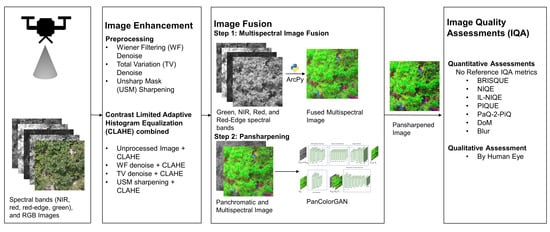
3. Materials and Methods

In our work, we combined different image preprocessing and fusion methods to overcome challenges in preserving spatial details and to improve spatial features of UAV images to detect plant stress. Therefore, the following sections describes where we gathered the data, how we preprocessed the images and which methods we used. In addition, the architecture of the used GAN and the quality assessment of the results via metrics is mentioned.

3.1. Dataset

An open dataset of multispectral potato images that was obtained from the University of Idaho’s Aberdeen Research and Extension Center [94] served as basis for our experiments. A low-altitude (3 m) unmanned aerial vehicle (UAV) equipped with a Parrot SEQUOIA+ multispectral camera featuring RGB sensors (3456 × 4608 pixels) and four monochrome sensors (960 × 1280 pixels), including green, red, red-edge, and near-infrared, was utilized by the researchers to capture images of potato plants. High-resolution RGB and multispectral images were cropped, rotated, and resized to extract image patches of 750 × 750 and 416 × 416 pixels, respectively. The first five rows and the field’s western edge received 50% less irrigation than the rest, resulting in stressed potato plants. The intention of the study [94] was to detect the water stress based on the captured UAV images.

Exemplary images from the dataset are depicted below in Figure 1:

3.2. Image Preprocessing

Image processing algorithms can change the image brightness, contrast, and sharpness, strongly affecting human and machine perception. In this study, the Wiener and total variation denoise filters were used for denoising, while the unsharp mask sharpening filters were utilized for deblurring.

3.2.1. Wiener Filtering (WF) Denoise

Wiener filtering is an efficient linear averaging algorithm for restoring degraded images from additive noise and blurring [95]. In this study, we employed an adaptive Wiener filter, which dynamically adjusts its behaviour based on the local variance present within the image. When encountering regions with high variance, indicative of significant noise or intricate details, the filter applies minimal smoothing to preserve these features. Conversely, in areas with low variance, suggesting smoother regions or less pronounced details, the filter applies more substantial smoothing. Notably, this adaptive approach facilitates the preservation of high-frequency details and edges within the image [96]. In this study, Wiener filtering is performed by the Scipy image processing library [97].

3.2.2. Total Variation (TV) Denoise

Total Variation (TV) denoise is an optimal solution for image denoising and retaining the sharp edges [98]. In this study, we opted for the utilization of Chambolle’s TV denoising algorithm [99], because of its faster computational performance and remarkable efficacy in dealing with synthetic Gaussian noises [100]. We implemented Chambolle’s algorithm through the utilization of the Scikit image restoration library [101], a well-established resource in the field of image processing.

3.2.3. Unsharp Mask (USM) Sharpening

Unsharp mask is a linear image improvement algorithm for enhancing the image’s contrast and sharpening the edges and other high-frequency details [102]. An unsharp masking filter works based on Equation (1):

$$ImprovedImage=Original+(Original-Blurred)\times amount.$$

(1)

According to Equation (1), the original image first is blurred. Then the original one is subtracted from the blurred one to obtain a high-contrast mask. Afterwards, the high-contrast mask is combined with the original images to enhance its sharpness. Moreover, the “$amount$” parameter plays a crucial role in contrast scaling, where the larger value leads to more of a sharpening effect.

The value of the “$amount$” parameter should be always $(amount\ge 1)$, where ($amount$ > 1) is referred to as Highboost Filtering, and $(amount<1)$ undervalued the unsharp masking. Selecting an appropriate $amount$ value is crucial for maintaining the balance between sharpening image details and over-enhancement; such as introduction image enhancement or a halo effect around the edges [103]. However, selecting the optimum $amount$ value is not a trivial task. Iterative experimentation and careful assessment are required to select the $amount$ value for a balance between image enhancement and the introduction of the image artifacts.

3.2.4. Contrast Limited Adaptive Histogram Equalization (CLAHE)

When images are processed, the uniformity of the images may decrease which results in non-uniform images. CLAHE is an algorithm that can alter the appearance of images by adjusting their brightness and contrast. It operates based on two parameters, including CLIP LIMIT and the BLOCK SIZE, with CLIP LIMIT resolving the issue of noise amplification by limiting the histogram’s value. In addition, BLOCK SIZE divides images into equal-sized, non-overlapping sub-sections. The CLAHE algorithm creates uniformity in the intensity distribution of images by employing the two functions listed above. Python’s OpenCV library was used to implement the algorithm, with a CLIP LIMIT of 3 and a BLOCK SIZE of 8*8. CLAHE was applied to all the images, including unprocessed and preprocessed images, the latter including Wiener filtering, total variation denoising, and unsharp masking. The components of the techniques and their combination are summarized in

Table 1. Image enhancement techniques with preprocessing and CLAHE integration.

Technique	Operators
Preprocessing	WF denoise
	TV denoise
	USM sharpening
CLAHE	Unprocessed Image + CLAHE
	WF denoise + CLAHE
	TV denoise + CLAHE
	USM sharpening + CLAHE

.

3.3. Image Enhancement

Image fusion is a significant part of image enhancement, where images from various sensors of the same scene are gathered and fused to produce enhanced, i.e., denoised, and more detailed images. In remote sensing, pansharpening is conducted by fusing low-resolution multispectral and high-resolution panchromatic satellite images in order to obtain such an enhanced, highly detailed image.

As previously applied mostly to satellite images, in this study a DL-based pansharpening approach utilizing a GAN has been adopted for enhancing UAV-based airborne images. The spectral bands are first fused to obtain a color composite of a multispectral image. Afterwards, the PAN and the MS images are fused by a color injection-based DL model, PanColorGAN [24], to yield spatially enhanced pansharpened images.

3.3.1. Multispectral Image Fusion

Four spectral images from green, near-infrared (NIR), red and red-edge channels were fused to obtain a highly detailed composite multispectral image, where the information from each spectral band will be merged (cf. Figure 2). A Python module named ArcPY [25] by ArcGIS pro was deployed in band co-registration.

The compositebands_ management function can successfully merge the spectral data from various sensors and produce a color composite of multispectral images. The color composite is beneficial in preserving all the details from individual bands. This module can produce square pixel output only [25]. However, in our case the size of the images is 416 × 416 pixels, which meets this requirement. Therefore, the output images have not been affected by unnecessary cropping.

3.3.2. Pansharpening

The 4-bands’ multispectral and panchromatic (PAN) images have been pansharpened by means of the self-supervised pansharpening model PanColorGAN [24]. The selected model was superior to the current CNN pansharpening networks because it succeeds in slowly upsampling and colorization of the low-resolution multispectral images and, thus, can effectively fuse it with the provided PAN images in order to avoid spatial detail loss. According to Ozcelik et al. [24], conventional CNN-based pansharpening approaches utilized the super-resolution task. Most of the super-resolution-based pansharpening approaches adopted the traditional MRA method (see Section 2.3), where the model attempts to implement the spatial details of the reduced-resolution panchromatic images into the spectral images during the training stage.

PanColorGAN, in contrast, employs the conventional CS-based pansharpening approach, where the model segregates multispectral images into spatial and spectral components and substitutes the spatial details of multispectral images with those derived from panchromatic images (see Section 2.3). The spatial details of the reduced-resolution panchromatic images were higher than the original multispectral images, which causes a spatial detail disagreement issue. Due to this disagreement, spatial details of the PAN images can get lost during the training phase. Accordingly, the generated pansharpened images suffered from a spatial detail loss compared to the original PAN images.

To avoid this spatial detail disagreement issue in the training phase, instead of using a reduced resolution PAN image, a grayscale multispectral image was provided, whose spatial details perfectly align with those of the original multispectral image. Consequently, our training dataset consisted of pairs comprising a grayscale multispectral image and its original multispectral counterpart, instead of the conventional pairings of PAN images and reduced-resolution multispectral data. During training, the model learns to separate the spatial and spectral details of the multispectral image and subsequently replace the spatial information of the multispectral image by the spatial information of the grayscale multispectral image.

In the testing phase, however, the original PAN images are input instead of the low-resolution grayscale multispectral images, which is considered as a spatial substitution between two images, that follows the CS-based approach.

3.3.3. Architecture Details

PanColorGAN, as the name indicates, uses the Generative Adversarial Network approach. The utilized implementation has been developed in the PyTorch framework. According to Figure 3, the training scheme can be described as follows: First, the multispectral ($Y_{MS}$) image is downsampled by k = 4×, and subsequently upsampled by by k = 4× to obtain $X_{MS}$ by bi-linear interpolation, which is a default setting of PanColorGAN architecture. On the other hand, $X_{MS}$ is then converted into the input format to obtain a single-channel grayscale signal $X_{GMS}$. Consequently, $X_{GMS}$ and $X_{MS}$ are fed into the generator network G and $\widehat{Y_G}$ is obtained as an output pansharpened image (cf. Figure 3).

The function of generator G is divided into four main parts, such as spatial detail extraction, color injection, transformation of features and finally image synthesis (cf. Figure 4).

The generator network (G) extracts the spatial features from a grayscale multispectral and PAN images. Then, the color from the multispectral images is injected into the PAN image before synthesizing it into the final pansharpened image by 3 × 3 convolutions. The residual block helps to transform the concatenated features and prepares them for final synthesis. Finally, the model obtains the feature from the detail extraction part and slowly increases the height and weight of the model by using upsampling and 3 × 3 convolution. For optimization, the activation function LeakyReLU and batch normalization are added after each convolutional layer. Furthermore, after obtaining features, the tanh activation function is used to map the image intensities to [−1, 1] interval to provide more stable and faster training.

The discriminator network (D) mimics the concept of Conditional Patch GAN [104] in that it uses the input images, ground truth, and generated images to distinguish between real and ‘fake’ images. After training in the inference stage when applied to (tested on) real-world images, the multispectral input images are first upsampled (by means of bi-linear interpolation operation) to match with the high-resolution PAN images. Then this pair is fed into the generator network (G) in order to obtain a full-resolution pansharpened image. Figure 5 illustrates this process.

3.3.4. Transfer Learning

In this study, we utilized Google Colab (https://colab.research.google.com/ (accessed on 4 August 2023)) which provided GPU support throughout the workflow. Specifically, we employed the Tesla T4 GPU with 16 GB of memory for the entire fusion process.

Our approach involved the utilization of a pre-trained PanColorGAN model on satellite images to enhance the spatial resolution of our Unmanned Aerial Vehicle (UAV) images through a process known as pansharpening.

In our testing phase, the input images (PAN and MS) were resized to 512 × 512 pixels by bi-linear interpolation to match the image size. The resized result was accomplished by downsampling and upsampling the PAN images ($X_{PAN}^{DOWN}$) and the MS images ($X_{MS}^{UP}$), respectively. Then the images were fed into the generator network G to obtain the final pansharpened image $\widehat{Y_{ps}}$ (cf. Figure 5).

3.4. Image Quality Assessments (IQA) Metrics

Being able to asses the quality of images is essential in image analysis tasks such as classification, object detection, image improvement and fusion. Considering the nature of images, their quality assessment, however, can be approached from two directions: subjective (or qualitative) or objective (or quantitative). In this work, both perspectives will be followed in Section 4 in order to evaluate the resulting images pansharpened by our proposed method.

In recent years, several types of objective image quality assessment (IQA) metrics, such as Full Reference (FR-IQA), Reduced Reference (RR-IQA), and No Reference (NR-IQA), have been proposed to calculate quantitative scores of images. For assessment using FR-IQA and RR-IQA, reference images are needed for comparison with the improved images. Since in our setting, the assumption of having access to reference images does not hold; in this work, we use several statistical, shallow ML- and deep-learning-based NR-IQA metrics in order to obtain objective, quantitative image scores. The resulting scores of such approaches are based on spatial details, blurriness, sharpness, and image contrast.

Due to the use of low-pass filters and image noise-reducing tasks, the images can become blurry. This potentially constitutes a problem for edge detection in images for modern image analysis tasks. Crété-Roffet et al. [105] developed no-reference blur evaluation metrics matching human perception. The blur metric ranges from 0 to 1, with 0 representing the best quality and 1 representing the worst quality. Therefore, lower values indicate higher quality [105]. The blur metric was computed using the Scikit image processing library [106].

On the other hand, the image can be blurred due to unstable sensor movement (e.g., shaky hands), defocus, and other image capture-related issues, which results in images with reduced sharpness. Kumar et al. [107] developed a metric called DoM, which can measure image sharpness by calculating the grayscale luminance values of the edges within the images. The sharpness score falls between 0 and $\sqrt{2}$, where lower scores indicate less sharp images [107]. This DoM sharpness score is calculated using a public Python library made available by the authors [108].

The Blind/Referenceless Image Spatial Quality Evaluator (BRISQUE) [109] is an opinion-aware (subjective human opinion score accompanied in the training process), NR-IQA method that evaluates images by a locally normalized luminance coefficients factor which measures the naturalness of the image. It is a holistic measure of the quality of the images instead of focusing on specific blurring, noises, and pixel blocking of the images. Despite its straightforward statistical model and low computational power demand, it outperforms the popular FR-IQA methods, such as locally normalized luminance coefficients and Structural Similarity Index (SSIM) [109]. BRISQUE scores generally range from 0 to 100, with lower scores indicating better image quality [109].

Natural Image Quality Evaluator (NIQE) on the other hand is an opinion-unaware NR-IQA metric based upon the Natural Scene Statistics (NSS) algorithm. It does not require human-modified images or human supervision to verify it [110]. Inspired by NIQE, another opinion-unaware NR-IQA method named Integrated Local NIQE (IL-NIQE) has been proposed. It deployed five NSS features, i.e., normalized luminance, Mean Subtracted and Contrast Normalized (MSCN) product, gradient, log-Gabor filter responses, and color statistics, which renders it more robust and feature-rich for image quality evaluation [111]. Both NIQE and IL-NIQE scores can range from 0 to infinity, with lower values indicating better image quality [110,111].

Similarly, the Perception-based Image Quality Evaluator (PIQUE) is a blind image evaluator that tries to evaluate the distortion without training images. The quality is measured by analyzing the spatial regions based on human perception by extracting block/patch features [112]. Typically, the PIQUE value ranges between 0 and 100. A lower value indicates better perceptual quality. An image is considered to have ’excellent’ perceptual quality when its PIQUE value falls between 0 and 20 [113].

Another DL-based image quality evaluator, Patches to Images (PaQ-2-PiQ), has been trained over the subjective score based on human perception. It can quantify the overall image quality, which matches perfectly with the human assessment. Other shallow-ML-based NR-IQA metrics can also accurately evaluate synthetically distorted images, however, are challenged by real-world datasets. On the other hand, PaQ-2-PiQ has been found to perform quite well with the naturally distorted dataset. The PaQ-2-PiQ metric spans from 0 to 100, where a higher score correlates with superior image quality [114].

For our quality assessment of the resulting images pansharpended by our proposed approach, the images’ BRISQUE, NIQE, and PIQUE metrics have been calculated with MATLAB^®’s image processing toolbox. In addition, IL-NIQE, and PaQ-2-PiQ have been calculated using a Python-based PyTorch image quality assessment (Pyiqa) library [115].

To further investigate the statistical significance of the difference among unprocessed, processed, and enhanced images, hypothesis tests have been conducted on 50 different samples. First, we performed the Shapiro–Wilk test [116] to confirm the normal distribution of the considered metrics. Afterwards, we performed the Tukey pairwise test [117] for cases of confirmed normal distribution and the non-parametric Mann–Whitney U test otherwise. The significance level $\alpha$ has been set to $0.05$.

The IQA metrics and their characteristics are summarized in

Table 2. Image quality metrics and characteristics.

Metrics	Characteristics
BRISQUE [109]	Holistic, uses luminance coefficients and human opinion scores.
NIQE [110]	NSS algorithm, opinion-unaware, no human-modified images.
IL-NIQE [111]	Robust, uses five NSS features for opinion-unaware assessment.
PIQUE [112]	Blind evaluator, assesses distortion without training images.
PaQ-2-PiQ [114]	Deep learning-based, trained on subjective scores, effective overall quality quantification.
DoM [107]	Measures sharpness through grayscale luminance values of edges.
Blur [105]	Evaluates blurriness using a no-reference metric, considers human perception.

.

4. Results

In the following, the spatial quality of unprocessed, preprocessed, and pansharpened images are reported and compared quantitatively and qualitatively. The quantitative results of the various NR-IQA metrics are summarized in

Table 3. Quantitative evaluation of Non-Reference Image Quality Assessment (NR-IQA) metrics for unprocessed, preprocessed multispectral, and pansharpened images of 50 image samples each. The table presents scores for various image quality metrics, including BRISQUE, NIQE, IL-NIQE, PIQUE, PaQ2PiQ, DoM, and blur, along with their respective standard deviations (±1 SD). Superscript letters (a, b, c, etc.) indicate statistical groupings for each metric, highlighting significant differences between the unprocessed, preprocessed multispectral, and pansharpened images, and the the best results are denoted as bold lettering. Abbreviations: UN: Unprocessed, MS: Multispectral, PS: Pansharpened, WF: Wiener Filtering, TV: Total Variation Denoise, USM: Unsharp Masking, CL: Contrast Limited Adaptive Histogram Equalization.

Methods		Metrics
		BRISQUE (± 1SD)	NIQE (± 1 SD)	IL-NIQE (± 1 SD)	PIQUE (± 1 SD)	PaQ2PiQ (± 1 SD)	DoM (± 1 SD)	Blur (± 1 SD)
Unprocessed RGB and Multispectral	RGB	43.40 ${ }^a$ ± 1.15	5.61 ${ }^a$ ± 0.57	24.06 ${ }^a$ ± 1.85	36.28 ${ }^a$ ± 4.91	67.74 ${ }^a$ ± 2.66	0.89 ${ }^a$ ± 0.02	0.37 ${ }^a$ ± 0.02
	UN MS	36.14 ${ }^b$ ± 2.55	4.69 ${ }^b$ ± 0.69	67.45 ${ }^b$ ± 7.58	11.34 ${ }^b$ ± 2.28	69.46 ${ }^b$ ± 2.20	0.97 ${ }^b$ ± 0.03	0.32 ${ }^b$ ± 0.02
Preprocessed Multispectral	MS WF	40.87 ${ }^c$ ± 2.20	5.51 ${ }^a$ ± 0.38	82.19 ${ }^c$ ± 7.31	32.20 ${ }^c$ ± 6.11	63.52 ${ }^c$ ± 1.18	0.84 ${ }^c$ ± 0.03	0.37 ${ }^a$ ± 0.02
	MS TV	40.70 ${ }^c$ ± 1.46	4.83 ${ }^b$ ± 0.36	61.24 ${ }^d$ ± 6.90	21.24 ${ }^d$ ± 6.00	69.50 ${ }^b$ ± 1.67	0.94 ${ }^d$ ± 0.03	0.34 ${ }^c$ ± 0.02
	MS USM	26.85 ${ }^d$ ± 3.53	4.13 ${ }^c$ ± 0.37	56.43 e ± 6.81	6.51 e ± 1.10	72.61 ${ }^d$ ± 1.68	1.08 e ± 0.02	0.25 ${ }^d$ ± 0.01
	MS CL	32.64 e ± 3.17	5.11 ${ }^b$ ± 1.40	86.21 ${ }^c$ ± 12.30	9.71 ${ }^b$ ± 2.44	73.25 ${ }^{de}$ ± 1.26	0.98 ${ }^b$ ± 0.03	0.30 e ± 0.02
	MS CL+WF	39.86 ${ }^c$ ± 1.73	5.78 ${ }^d$ ± 1.78	95.31 ${ }^f$ ± 9.61	25.96 ${ }^f$ ± 5.35	67.57 ${ }^a$ ± 1.18	0.85 ${ }^c$ ± 0.02	0.33 ${ }^{bc}$ ± 0.02
	MS Cl+USM	32.20 e ± 5.13	5.23 ${ }^{abd}$ ± 1.04	88.71 ${ }^c$ ± 12.31	8.49 ${ }^{be}$ ± 2.32	76.25 ${ }^f$ ± 0.97	1.05 ${ }^f$ ± 0.03	0.26 ${ }^d$ ± 0.01
	MS CL+TV	37.31 ${ }^b$ ± 2.68	5.56 ${ }^{abd}$ ± 0.35	75.31 ${ }^g$ ± 9.79	16.57 ${ }^g$ ± 4.53	72.28 ${ }^d$ ± 1.27	0.96 ${ }^{bd}$ ± 0.03	0.33 ${ }^{bc}$ ± 0.02
Unprocessed and Preprocessed Pansharpened	UN PS	36.13 ${ }^b$ ± 1.68	5.06 ${ }^b$ ± 0.58	58.64 ${ }^{de}$ ± 8.13	25.86 ${ }^f$ ± 2.86	72.99 ${ }^{de}$ ± 0.68	0.95 ${ }^{bd}$ ± 0.02	0.30 e ± 0.01
	PS WF	38.6 ${ }^b$ ± 1.92	5.32 ${ }^{bd}$ ± 0.57	60.29 ${ }^d$ ± 7.00	36.45 ${ }^a$ ± 2.39	69.92 ${ }^{bc}$ ± 1.66	0.86 ${ }^c$ ± 0.03	0.33 ${ }^{bc}$ ± 0.02
	PS TV	37.97 ${ }^b$ ± 1.80	5.18 ${ }^{bd}$ ± 0.59	55.71 e ± 7.362	40.57 ${ }^h$ ± 3.52	72.00 ${ }^g$ ± 0.87	0.91 ${ }^h$ ± 0.03	0.32 ${ }^{be}$ ± 0.02
	PS USM	27.58 ${ }^d$ ± 1.97	4.57 e ± 0.57	49.67 ${ }^h$ ± 8.09	10.94 ${ }^b$ ± 1.05	77.56 ${ }^h$ ± 0.51	1.03 ${ }^i$ ± 0.01	0.26 ${ }^d$ ± 0.01
	PS CL	42.88 ${ }^a$ ± 1.96	6.19 ${ }^f$ ± 0.69	70.42 ${ }^b$ ± 9.89	29.68 ${ }^c$ ± 4.17	73.50 e ± 0.71	0.90 ${ }^a$ ± 0.02	0.30 e ± 0.01
	PS CL+WF	42.17 ${ }^{ac}$ ± 2.14	6.07 ${ }^f$ ± 0.63	74.13 ${ }^g$ ± 9.45	40.58 ${ }^h$ ± 3.57	71.16 ${ }^d$ ± 1.02	0.96 ${ }^{bd}$ ± 0.01	0.32 e ± 0.01
	PS CL+TV	43.02 ${ }^a$ ± 1.52	6.09 ${ }^f$ ± 0.67	66.31 ${ }^b$ ± 10.08	36.94 ${ }^a$ ± 3.97	73.10 ${ }^{de}$ ± 0.77	1.03 ${ }^i$ ± 0.01	0.32 ${ }^{bce}$ ± 0.01
	PS CL+USM	34.16 ${ }^f$ ± 2.98	4.57 ${ }^g$ ± 0.57	72.83 ${ }^g$ ± 10.80	16.60 ${ }^g$ ± 2.24	75.16 ${ }^i$ ± 0.53	0.98 ${ }^b$ ± 0.01	0.26 ${ }^d$ ± 0.01

. The entries in the table reflect the means of the metrics over all images in the dataset. The dataset contains 360 multispectral images.

Figure 6 and Figure 7 are additionally presented to allow for qualitative inspection. In this section, $UNRGB$, $UNMS$, and $UNPS$ refer to the unprocessed RGB, multispectral, and pansharpened images, respectively. $WF$, $TV$, $USM$, and $CL$ represent the preprocessed images with the Wiener filter, total variance, unsharp masking, and CLAHE algorithm, respectively.

4.1. Quantitative Assessment

We compared numerous combinations of unprocessed, preprocessed, and enhanced images in terms of the BRISQUE, NIQE, IL-NIQE, PIQUE, PaQ2PiQ, DoM, and blur metrics to quantify the spatial quality of images in Table 3. A lower score means better perceptual quality for BRISQUE, NIQE, IL-NIQE, PIQUE, and blur metrics. On the other hand, in PaQ2PiQ, and DOM metrics, a higher score indicates better perceptual quality.

MS USM scored best (i.e., lower) compared to all images in terms of the BRISQUE metric. However, no statistically significant difference has been found with PS USM $(p>0.05)$. In the case of NIQE metrics, MS USM shows significantly $(p<0.05)$ improved spatial details than the other images. On the other hand, RGB exhibited a significantly higher spatial quality according to IL-NIQE measurements. Regarding PIQUE metrics, MS USM images evaluate better on average than the other images. However, no significant difference has been found with MS CL+USM $(p>0.05)$. Regarding human perception-based quantification, PS USM resulted in significantly $(p<0.05)$ better image quality metrics as calculated by the PaQ-2PiQ. According to the DoM metrics, MS USM has scored for significantly $(p<0.05)$ better sharpness. Regarding the blur metrics, MS USM images have revealed less blurriness, but no statistically significant difference when compared to MS CL+USM, PS USM, and PS CL+USM $(p>0.05)$.

On the other hand, UN RGB possessed the least spatial quality in terms of BRISQUE metrics, but no significant difference has been found when compared with PS CL, PS CL+WF, and PS CL+TV $(p>0.05)$. Considering the NIQE metrics, PS CL resulted in lower image quality, with no significant differences between PS CL+WF and PS CL+TV $(p>0.05)$. According to IL-NIQE metrics, MS CL+WF has the lowest spatial quality. The score differed significantly from the other variants of the images $(p<0.05)$. PS CL+WF results in a lower perceptual quality in terms of the PIQUE metric, where no significant difference can be confirmed compared to PS TV $(p>0.05)$. In the case of PaQ2PiQ metrics, MS WF shows a lower image quality. However, no significant difference has been found to PS WF $(p>0.05)$. MS WF also resulted in a lower sharpness score, as measured by the DoM metric. Nevertheless, MS WF again no significant differences when compared with MS CL+WF and PS WF $(p>0.05)$ have become apparent. In blur metrics, UN RGB and MS WF exhibited the most blurry image output, with no significant differences between each other $(p>0.05)$.

In summary, MS USM outperformed all other images in terms of the BRISQUE metric, showcasing superior quality. NIQE metrics revealed MS USM’s significantly enhanced spatial details, while RGB excelled in spatial quality according to IL-NIQE measurements. Moreover, MS USM demonstrated better overall performance in PIQUE metrics and human perception-based quantification, with notable improvements in sharpness and reduced blurriness. Conversely, UN RGB displayed the lowest spatial quality, albeit without significant differences compared to certain variants. In image preprocessing, PS CL exhibited lower image quality across various metrics, while MS CL+WF showed the least spatial quality. Despite these variations, some comparisons did not yield statistically significant differences.

4.2. Qualitative Assessment

To complement the quantitative evaluation from the previous section, we now focus on a concrete example images depicted in Figure 6 and Figure 7 and rate their quality based on subjective (qualitative) properties.

The PAN image is constructed from the RGB image and has a spatial resolution of 750 × 750 pixels. The multispectral images (7–14) represent a color composite derived from spectral bands (3–6), where UN MS (7) is derived from the unprocessed spectral bands and the multispectral images (8–14) are the output of various preprocessed spectral bands. Similarly, the pansharpened images (15–22) were generated with PanColorGAN by fusing the unprocessed and preprocessed PAN (1) and the multispectral images (7–14).

The red box in Figure 6 was used to emphasize the structural similarities and differences among the images. Similarly, the red box in Figure 7 is used to focus and highlight the images’ color difference and edge sharpness.

In Figure 6, spectral images (3–6) had structural dissimilarities inside the red box. Focusing the green spectral band as a reference image for now, the multispectral images have been fused into a color composite of MS images, which contains the spectral information from all of the spectral bands and follows the structure of the green band. The merged details from the spectral bands render the MS images structurally prominent and chromatically detailed. The unsharp mask-filtered image (9) displayed more sharp leaf edges. On the other hand, MS WF (8) and MS TV (10) provided a blurry appearance. The PS images (15–18) obtained the structure of the MS images. The PS images were chromatically more natural, and the structure and edges of the leaves appear sharper. The PS WF (16) images visually exhibit more blur than the UN PS (15), while PS USM (17) had sharp features which can be seen prominently in the leaf edges. Conversely, the CLAHE-preprocessed MS images (11–14) suffered from chromatic distortion, resulting in undesirable color artifacts at the image edges. Since PANColorGAN incorporates colors from the MS images, the PS images (15–22) also exhibited this chromatic distortion issue.

In Figure 7, the red box marked the color differences between the small round shadow and the leaf foliage. Similar to Figure 6, the MS color composite was generated by following the structure of the green spectral bands (3). The color composite of multispectral images clearly distinguishes the spectral difference between the shadow and the leaf foliage, where the shadow was purplish, and the leaves were green. MS WF (8) and MS TV (10) show blurry images. On the other hand, MS USM (9) has been found sharper than the other multispectral images. In the case of the PS images (15–18), the canopy structure of the potato plants was sharper, and the small shadow can also be clearly distinguished in comparison with the MS images. The edges of the small leaves of PS USM (17) are sharper and more distinguishable. Similar to Figure 6, CLAHE preprocessed MS (11–14) and PS images (19–22), both MS and PS have been found to face the color distortion issue, which is not the case for the combination of other preprocessing techniques.

5. Discussion

Our study investigated the effectiveness of image-fusion methods, more precisely pansharpening, regarding the preservation of high spatial information of PAN images for the transfer to MS images. It further evaluates the impact of several image preprocessing algorithms applied to the PAN image on the examined GAN-based approach’s capability to improve both the spatial as well as the color properties. In the following section, our results are critically examined and contextualized to the current state-of-the-art.

To start with the image-fusion methods, this study determined that the presented color injection-based pansharpening approach can combine the information from the PAN images and all spectral bands without sacrificing the images’ spatial details. Furthermore, images preprocessed with more conventional image filters have been found to impose certain effects on the fusion quality and spatial details of the resulting pansharpened images. Among the filters applied in image preprocessing steps, unsharp mask filters were revealed to have the overall better capability to preserve the sharpness and features in the pansharpened images. The final pansharpened images have been evaluated by means of quantitative metrics and qualitatively based on the visual assessment of two exemplary images from the case study dataset containing low-altitude multispectral potato images. The pansharpened images were compared with the PAN images as well as unprocessed and preprocessed multispectral images in order to determine how much spatial quality the images gained or lost. NR-IQA metrics scores were used for the quantitative evaluation.

According to the BRISQUE metric, the pansharpened images’ overall spatial scores were similar to the multispectral images and better than the RGB images, which is interpreted as a positive indication of the presented approach’s capability to preserve the spatial quality. According to Ozcelik et al. [24], blurriness was one of the major problems of the synthetically generated, i.e., pansharpened, images. However, our PS images that have been improved by combining with targeted preprocessing techniques revealed less blur in the corresponding metrics than the unprocessed RGB and MS images. Moreover, the unsharp masking algorithm improved images by enhancing the overall spatial details and at the same time by reducing blurriness, as became apparent by looking at the BRISQUE and blur metrics.

Although NIQE and IL-NIQE were calculated based on NSS features, the spatial scores of the images are quite different. In terms of the NIQE metric, the GAN-enhanced UN PS images scored for better image quality than the UN RGB images. However, no statistically significant difference was found between the NIQE scores of UN PS and UN MS $(p>0.05)$. Moreover, the positive impact of the unsharp mask algorithm was observable in the NIQE’s score. Interestingly, in terms of IL-NIQE, the RGB image have been found to possess better spatial quality than the others, which contradicts the result of other evaluation metrics. This is due to the fact that IL-NIQE has been developed on the five major features of the NSS, which denotes its robustness of measuring natural scenes of the images. The color feature of the IL-NIQE boosted its capacity to determine the quality of the natural scene of the images. A MultiVariate Gaussian (MVG) model was trainedto generate a representation of those NSS features of the natural images, and the pristine MVG model serves as a reference to evaluate the capacity of a given image [118]. Hence, any artificially distorted and computer-generated images exhibited lesser spatial details of the images. In the dataset, all images were computer generated with artificial coloring except the RGB image. Consequently, the RGB image processes the best quality scores in IL-NIQE metrics, which indicates its naturalness as well. However, compared with the UN MS, UN PS showed better image quality in terms of naturalness, measured by the NSS features. Furthermore, PS USM had the second-best image quality in IL-NIQE metrics, which corroborates the observed robustness of the combination of PanColorGAN and the unsharp masking filters in inducing the naturalness of the fused images. These findings indicated a strong correlation with and thus substantiate the insights from the qualitative assessment of the images.

A PIQUE value between 0 and 20 denotes an image’s “excellent” perceptual quality [113]. The average PIQUE value of the PS images was revealed to be 25.86. Furthermore, the score even increased when applying the unsharp masked preprocessing for the finally pansharpened images.

The PaQ-2-PiQ metric is a standard ground evaluation of local and global image quality, which on the one hand, can score the images based on the Region of Interest Pooling (RoIPool) method, which is used to extract small feature maps within an image, and, on the other hand, can merge the global feedback to calculate precise subjective scores. According to PaQ-2-PiQ, PS has had almost similar scores to MS USM, while MS USM already outperformed in the BRISQUE, NIQE, PIQUE, DoM, and blur metrics. Here, PS USM has the highest significant image quality. This result also indicates the profound effect of unsharp masking filtering in improving the spatial quality of the PS images.

On the other hand, both denoising filters, such as Wiener and total variation denoising filters, struggled with removing the noise from the dataset and imported unnecessary blurriness and reduced sharpness. In every metric, the Wiener and total variation denoising filters had a lower level of spatial image quality. However, the denoising algorithms faced challenges in removing real-world noise and preserving the image details. Anam et al. [119] also found that the Wiener denoising filter cannot preserve the spatial details of the images after denoising. According to the review of Buades et al. [120], TV denoise faced challenges in preserving the images’ details and edges.

On the contrary, in several studies, it was found that classical denoising filters work well for removing artificially added noise. For example, classical image restoration filters can successfully remove artificially added noises in remotely sensed images [121], and in the medical images domain [122]. From the above arguments, it becomes apparent that the Wiener and total variation denoise images only work with certain artificially added noises. Since we did not induce any artificial noise in the dataset, Wiener and total variation denoise filters could not be found helpful in improving image quality for our case study. Our observations confirm that the image denoising algorithm has no positive effect for improving the spatial image quality of the pansharpened images. Furthermore, it degraded the image quality. On the other hand, unsharp mask filters significantly improved the image quality of the fused images according to the respective metrics. Our findings conform with those of the study of Liu et al. [123], where the authors found the image details and contrast improvement of the remotely sensed images using unsharp masking.

The quantitative scores of the CLAHE-applied images showed positive values in NR-IQA metrics. For example, PIQUE’s score indicated that MS CL, MS CL + USM, MS CL + TV, and PS CL + USM are perceptually “excellent” and have less blurriness and higher sharpness. However, in Figure 6 and Figure 7, CLAHE preprocessed images showed color distortions and extra colors compared to other input images. In [124], Malik et al. also found that the CLAHE algorithm leads to distortions of the image’s color.Hu et al. [125] also found that CLAHE-applied images can experience an oversaturation issue. Therefore, despite having good quantitative scores of CLAHE processed images, they were color-distorted and complex to distinguish visually (cf. Figure 6 and Figure 7). On the other hand, Zheng et al. [126] discovered that applying CLAHE on PAN images improved the quality of pansharpened images. Instead of preprocessing the CLAHE approach on the spectral bands, applying it solely to the PAN images might help to reduce the color distortion issue.

In pansharpening, qualitative analysis is one of the most critical evaluation techniques of the images. The human visual system can compare image contrast, chromatic preservation, and image detail to determine which image is superior. The acutance of the images, which is a measure of the contrast of the edges, is an additional essential component of qualitative analysis of the images. As there is no unit for measuring the acutance of images, it cannot be quantified. The higher the edge contrast, the more distinct an image’s edges appear to the human visual system [127]. In addition, Masi et al. [128] found that higher quantitative scores were not always associated with superior perceptual quality of photos.

The visual characteristics of the images were compared using Figure 6 and Figure 7. In Figure 6, within the red box, the contrast between the small round shadow and the green pixels of the leaves in the RGB image was nearly indistinguishable. In the red spectral bands, the spectral difference between the shadow and the leaves was minimal; however, in the NIR band, it was significant. Additionally, green spectral images showed occurrences of motion-blurring difficulties. The chromatic dissimilarity between the leaves, shadows, and soil was visible after merging all spectral bands into a color composite of the multispectral image. Visually, the sharper edges and the contrast of the pansharpened images were more easily detectable than the multispectral images. Moreover, in the pansharpened images, just beneath the red box, the sharp contrast differences among the green pixels indicated less dense foliage in Figure 6.

Compared with the multispectral images, the edge contrast of the little leaves is more prominent in the pansharpening images. In PS WF, undesirable artifacts such as image ringing are observable that degrade the image quality. In the quantitative metrics, it has already been demonstrated that USM leads to higher spatial features compared to others; visually, it can be seen as a better sharpness compared to others. Therefore, the USM filter can improve the sharpness of pansharpened images. Khan et al. [127] also discovered that images preprocessed with the sharpness filter enhanced the quality of pansharpened images. Teke et al. [129] pansharpened the satellite images with the sharpened PAN image, which again improved the spatial quality of the images. In terms of color preservation, no dramatic effect of the WF, TV, and USM filters was observed on the pansharpened images. On the other hand, PanColorGAN was able to preserve the color of the input multispectral images. Additionally, it introduced the naturalness to the chromatic quality of the pansharpened images (15–18) (cf. Figure 6 and Figure 7), which perfectly aligns with the quantitative scores of the IL-NIQE matrices Table 3.

In Figure 6, inside the red box, geometrical dissimilarities were noticeable among the PAN and spectral bands. Green (3) and red band (5) images differ structurally from NIR (4) and the red-edge band (6) images. In image fusion, it was challenging for the fusion algorithms to match the feature of different structures and fuse them correctly, which might introduce unwanted features in the reference image and produce misregistered and blurry fused images [23]. The slight blurriness of the fused multispectral images (7) resulted from the differently structured spectral bands. Li et al. [130] discussed a similar remote-sensing image-fusion issue. In order to address the geometrical variations in the spectral bands, it is necessary to capture images carefully and choose the most adequate image-fusion algorithm.

We have used the ArcPy Python module of ArcGIS to merge the spectral bands, which were developed in the context of the satellite images. However, our images were low-altitude UAV images. We have seen the geometrical differences among the spectral bands that challenged the applied fusion model to combine the spectral information correctly.

Moreover, the PanColorGAN network used for pansharpening was originally trained on a satellite image dataset. Further, while comparing the pansharpened images against RGB, some missing pixels became apparent. For further comparison, our output image was compared against Brovey transform-based pansharpening (see Figure 8). In the red circle, white flowers in the RGB images can be detected. However, both pansharpened images failed to import the flower structure. Such so-called object disappearance issues should be more thoroughly considered when designing a new pansharpening model for low-altitude UAV photos in the future.

Considering again the preprocessing techniques, the image-denoising algorithms could not successfully counteract naturally occurring noise sources properly, which is considered a major limitation of those algorithms. On one hand, there may be an issue with providing denoising filters in general, as in real-world scenarios, when datasets are large, various images may exhibit different types of noise issues stemming from the image capture process. On the other hand, instead of using classical image denoising algorithms, DL-based blind denoising method could be a viable option for real-world scenarios (see Section 2.3). For example, CBDNet [131], a blind-image denoising approach, was trained on a Poisson-Gaussian noise model for the raw images captured by imaging sensors and the complex noise present in real-world images after image processing. Furthermore, the noise distribution in real-world image datasets is not always Gaussian; it can be more complex. Consequently, Gaussian denoisers often perform poorly. To address this issue, a hybrid technique combining classical denoisers and DL-based methods could be applicable [132].

Furthermore, motion blur constitutes one of the major issues of UAV-captured images. We deem blind motion deblurring algorithms promising to alleviate the negative impacts of such degraded images on subsequent image analysis tasks. However, there is a limitation on the DL-based deblurring technique, because most of the image deblurring algorithms are trained on a pair of real-world GT images and a synthetically blurred image, which performs well on the synthetically blurred images, and failed miserably on the real-world blurred images. Moreover, real-world blurred images not only bring blurred artifacts but also suffer from noises, hence, one unifying image restoration algorithm would be a better choice in real-world scenarios [75].

Additionally, we employed the ArcPy tool for spectral band fusion, which successfully merged the spectral bands. However, it inadvertently introduced non-realistic colors to the images. This could be attributed to the tool’s development, which primarily targeted high-altitude satellite imagery. To address this issue in future endeavors, research should prioritize a spectral band merging technique that emphasizes guided colorization and feature preservation of low-altitude UAV spectral bands. In addition to band merging, it seems promising to intensify the work towards developing further improved DL models for specifically pansharpening low-altitude UAV-captured images from the crop production domain.

Moreover, the original PanColorGAN model was mainly developed to address the issues of guided colorization and the preservation of spatial details, and ignored to focus on spectral details. Additionally, spectral image details are the important features for the remote-sensing images. Hence, in a future study, the research will focus on a model that focuses on the both spatial and spectral detail improvements.

Furthermore, in image processing, evaluations can be both image-specific and task-specific. We employed NR-IQA-based evaluation metrics as part of the image-specific evaluation method. For task-specific evaluation, the enhanced images are utilized in various machine learning- (ML) and deep learning (DL)-based downstream tasks, such as image classification, object detection, and instance segmentation, to assess whether accuracy of the DL-based models improves or not. However, employing both methods of evaluation would be time-consuming. Therefore, implementation and comparison of various downstream tasks would be a part of another research study.

Moreover, the adoption of DL models specifically developed for image enhancement and trained on low-altitude UAV-based multispectral agricultural image datasets appears to be in its infancy.Due to the lack of open-source low-altitude multispectral UAV image datasets, comparing them with different datasets is out of the scope right now. Although, collecting low-altitude multispectral UAV dataset is a time-consuming task; in a future study we will explore the opportunity to collect and test the different dataset of different crops and environmental conditions.

6. Conclusions

Unmanned aerial vehicles (UAVs) are used in several agricultural applications, such as the detection of stress or pathogens. While operating in a natural environment, UAVs have to adapt to different challenging conditions, such as changing light conditions or windy weather. Although UAVs can provide images with a higher spatial resolution compared to satellites, the image quality can heavily vary because of blurriness or noise. This can lead to unsatisfactory image quality, which we intend to improve based on the PanColorGAN approach.

The study presented a combination of image preprocessing and fusion methods to improve the spatial features of the UAV images for plant stress detection. The research was motivated to address the challenges of preserving spatial details by image-fusion algorithms. Furthermore, to find out the effect of the image preprocessing filters on improving image sharpness, contrast, and edges. Considering spatial quality degradation as the pansharpening problem, the image preprocessing task was proposed to produce better spatially improved pansharpened images. For image preprocessing, Wiener denoise, total variance denoise, and unsharp mask sharpening filters were used. Moreover, CLAHE was applied to the unprocessed and filtered images to fix image contrast. First, the spectral bands were fused into multispectral images for image fusion. For the pansharpening process, the panchromatic and the multispectral images were fused using a color injection-based DL model called, PanColorGAN. In our study, the generated pansharpened images had better image details, sharpness, and more distinguished image edges. Among the preprocessing techniques, unsharp mask sharpening improved the image details, contrast, and sharpness. However, the other image-denoising algorithms faced challenges in improving the image quality, rather ended up with blurry and degraded images. Moreover, CLAHE preprocessed images had better quantitative scores in some metrics, but the images faced major chromatic distortion issues. Due to the geometrical dissimilarities of the spectral bands, the fused multispectral images faced a small object missing issue. Finally, during pansharpening, the model struggled to import the small object from the PAN images.

The innovative character of the study consists of applying Generative Artificial Intelligence for producing high quality low-altitude images. As our literature review reveals, existing research primarily focuses on satellite images. From this follows a lack of studies about the improvement of low-altitude images. The approach of using Generative Artificial Intelligence to fuse low-altitude images as of yet has not received enough attention in the literature. The investigated combination with conventional methods shows an improvement in NR-IQA metrics.Therefore, our study also supports the enhancement of image quality in low-altitude images for following Artificial Intelligence tasks. Another contribution of our work is to obtain the first insights regarding the question of to what extent the application of Generative Artificial Intelligence combination with conventional image processing algorithms allows for quality improvements of multispectral images in the context of our considered use case (UAV-based inspection of potato plants).

For future work, DL-based state-of-the-art blind image denoising and motion deblurring algorithms should be implemented in image preprocessing task. On the other hand, two image-fusion models need to be developed in the future, which will solely focus on low-altitude UAV images. One will be for the spectral band fusions and another for pansharpening. PanColorGAN effectively completed the pansharpening process while maintaining the color and spatial characteristics of the images. A pansharpening model that shares a common ground for improving spatial and spectral features should be considered in future research. The absence of diverse low-altitude multispectral UAV data hindered our ability to compare the method across various crops and diverse environmental settings. Thus, for future research endeavors, it is imperative to gather additional data pertaining to similar agricultural use cases and conduct comparative analyses among them.

References

1. Lipiec, J.; Doussan, C.; Nosalewicz, A.; Kondracka, K. Effect of drought and heat stresses on plant growth and yield: A review. Int. Agrophys. 2013, 27, 463–477. [Google Scholar] [CrossRef]
2. Oshunsanya, S.O.; Nwosu, N.J.; Li, Y.; Oshunsanya, S.O.; Nwosu, N.J.; Li, Y. Abiotic stress in agricultural crops under climatic conditions. In Sustainable Agriculture, Forest and Environmental Management; Springer: Singapore, 2019; pp. 71–100. [Google Scholar] [CrossRef]
3. Savci, S. Investigation of Effect of Chemical Fertilizers on Environment. APCBEE Procedia 2012, 1, 287–292. [Google Scholar] [CrossRef]
4. Bongiovanni, R.; Lowenberg-Deboer, J. Precision agriculture and sustainability. Precis. Agric. 2004, 5, 359–387. [Google Scholar] [CrossRef]
5. Maimaitiyiming, M.; Ghulam, A.; Bozzolo, A.; Wilkins, J.L.; Kwasniewski, M.T. Early Detection of Plant Physiological Responses to Different Levels of Water Stress Using Reflectance Spectroscopy. Remote Sens. 2017, 9, 745. [Google Scholar] [CrossRef]
6. Walter, A.; Finger, R.; Huber, R.; Buchmann, N. Smart farming is key to developing sustainable agriculture. Proc. Natl. Acad. Sci. USA 2017, 114, 6148–6150. [Google Scholar] [CrossRef]
7. Steven, M.D.; Clark, J.A. Applications of Remote Sensing in Agriculture; Elsevier: Amsterdam, The Netherlands, 2013. [Google Scholar]
8. Chiu, M.T.; Xu, X.; Wei, Y.; Huang, Z.; Schwing, A.G.; Brunner, R.; Khachatrian, H.; Karapetyan, H.; Dozier, I.; Rose, G.; et al. Agriculture-Vision: A Large Aerial Image Database for Agricultural Pattern Analysis. In Proceedings of the IEEE/CVF Conference on Computer Vision and Pattern Recognition (CVPR), Seattle, WA, USA, 13–19 June 2020; pp. 2828–2838. [Google Scholar]
9. Sieberth, T.; Wackrow, R.; Chandler, J.H. Automatic detection of blurred images in UAV image sets. ISPRS J. Photogramm. Remote Sens. 2016, 122, 1–16. [Google Scholar] [CrossRef]
10. Wang, R.; Xiao, X.; Guo, B.; Qin, Q.; Chen, R. An Effective Image Denoising Method for UAV Images via Improved Generative Adversarial Networks. Sensors 2018, 18, 1985. [Google Scholar] [CrossRef] [PubMed]
11. Jeong, E.; Seo, J.; Wacker, J.P. UAV-aided bridge inspection protocol through machine learning with improved visibility images. Expert Syst. Appl. 2022, 197, 116791. [Google Scholar] [CrossRef]
12. Kwak, G.H.; Park, N.W. Impact of Texture Information on Crop Classification with Machine Learning and UAV Images. Appl. Sci. 2019, 9, 643. [Google Scholar] [CrossRef]
13. Maini, R.; Aggarwal, H. Study and comparison of various image edge detection techniques. Int. J. Image Process. (IJIP) 2009, 3, 1–11. [Google Scholar]
14. Motayyeb, S.; Fakhri, S.A.; Varshosaz, M.; Pirasteh, S.; Motayyeb, S.; Fakhri, S.A.; Varshosaz, M.; Pirasteh, S. Enhancing Contrast of Images to Improve Geometric Accuracy of a Uav Photogrammetry Project. Int. Arch. Photogramm. Remote Sens. Spat. Inf. Sci. 2022, 43-B1, 389–398. [Google Scholar] [CrossRef]
15. Hung, S.C.; Wu, H.C.; Tseng, M.H. Integrating image quality enhancement methods and deep learning techniques for remote sensing scene classification. Appl. Sci. 2021, 11, 11659. [Google Scholar] [CrossRef]
16. Milanfar, P. A tour of modern image filtering: New insights and methods, both practical and theoretical. IEEE Signal Process. Mag. 2012, 30, 106–128. [Google Scholar] [CrossRef]
17. Al-amri, S.S.; Kalyankar, N.V.; Khamitkar, S.D. Contrast Stretching Enhancement in Remote Sensing Image. BIOINFO Sens. Netw. 2011, 1, 6–9. [Google Scholar]
18. Thomas, C.; Ranchin, T.; Wald, L.; Chanussot, J. Synthesis of multispectral images to high spatial resolution: A critical review of fusion methods based on remote sensing physics. IEEE Trans. Geosci. Remote Sens. 2008, 46, 1301–1312. [Google Scholar] [CrossRef]
19. Fonseca, L.; Namikawa, L.; Castejon, E.; Carvalho, L.; Pinho, C.; Pagamisse, A.; Fonseca, L.; Namikawa, L.; Castejon, E.; Carvalho, L.; et al. Image Fusion for Remote Sensing Applications. In Image Fusion and Its Applications; IntechOpen: London, UK, 2011. [Google Scholar] [CrossRef]
20. Kremezi, M.; Kristollari, V.; Karathanassi, V.; Topouzelis, K.; Kolokoussis, P.; Taggio, N.; Aiello, A.; Ceriola, G.; Barbone, E.; Corradi, P. Pansharpening PRISMA Data for Marine Plastic Litter Detection Using Plastic Indexes. IEEE Access 2021, 9, 61955–61971. [Google Scholar] [CrossRef]
21. Karakus, P.; Karabork, H. Effect of Pansharpened Image on Some of Pixel Based and Object Based Classification Accuracy. Int. Arch. Photogramm. Remote Sens. Spat. Inf. Sci. 2016, XLI-B7, 235–239. [Google Scholar] [CrossRef]
22. Chen, F.; Lou, S.; Song, Y. Improving object detection of remotely sensed multispectral imagery via pan-sharpening. In Proceedings of the ICCPR 2020: 2020 9th International Conference on Computing and Pattern Recognition, Xiamen, China, 30 October–1 November 2020; ACM International Conference Proceeding Series. ACM: New York, NY, USA, 2020; pp. 136–140. [Google Scholar] [CrossRef]
23. Xu, Q.; Zhang, Y.; Li, B. Recent advances in pansharpening and key problems in applications. Int. J. Image Data Fusion 2014, 5, 175–195. [Google Scholar] [CrossRef]
24. Ozcelik, F.; Alganci, U.; Sertel, E.; Unal, G. Rethinking CNN-Based Pansharpening: Guided Colorization of Panchromatic Images via GANs. IEEE Trans. Geosci. Remote Sens. 2021, 59, 3486–3501. [Google Scholar] [CrossRef]
25. ArcGIS API for Python—ArcGIS Pro|Documentation; Esri: Redlands, CA, USA, 2023.
26. Haridasan, A.; Thomas, J.; Raj, E.D. Deep learning system for paddy plant disease detection and classification. Environ. Monit. Assess. 2023, 195, 120. [Google Scholar] [CrossRef]
27. Bhujade, V.G.; Sambhe, V. Role of digital, hyper spectral, and SAR images in detection of plant disease with deep learning network. Multimed. Tools Appl. 2022, 81, 33645–33670. [Google Scholar] [CrossRef]
28. Wang, A.; Zhang, W.; Wei, X. A review on weed detection using ground-based machine vision and image processing techniques. Comput. Electron. Agric. 2019, 158, 226–240. [Google Scholar] [CrossRef]
29. Arsenovic, M.; Karanovic, M.; Sladojevic, S.; Anderla, A.; Stefanovic, D. Solving Current Limitations of Deep Learning Based Approaches for Plant Disease Detection. Symmetry 2019, 11, 939. [Google Scholar] [CrossRef]
30. Barbedo, J.G.A. A review on the main challenges in automatic plant disease identification based on visible range images. Biosyst. Eng. 2016, 144, 52–60. [Google Scholar] [CrossRef]
31. Di Cicco, M.; Potena, C.; Grisetti, G.; Pretto, A. Automatic model based dataset generation for fast and accurate crop and weeds detection. In Proceedings of the 2017 IEEE/RSJ International Conference on Intelligent Robots and Systems (IROS), Vancouver, BC, Canada, 24–28 September 2017; pp. 5188–5195. [Google Scholar] [CrossRef]
32. Labhsetwar, S.R.; Haridas, S.; Panmand, R.; Deshpande, R.; Kolte, P.A.; Pati, S. Performance Analysis of Optimizers for Plant Disease Classification with Convolutional Neural Networks. In Proceedings of the 2021 4th Biennial International Conference on Nascent Technologies in Engineering (ICNTE), Navi Mumbai, India, 15–16 January 2021; pp. 1–6. [Google Scholar]
33. Barbedo, J.G.A.; Koenigkan, L.V.; Santos, T.T.; Santos, P.M. A Study on the Detection of Cattle in UAV Images Using Deep Learning. Sensors 2019, 19, 5436. [Google Scholar] [CrossRef]
34. Wen, D.; Ren, A.; Ji, T.; Flores-Parra, I.M.; Yang, X.; Li, M. Segmentation of thermal infrared images of cucumber leaves using K-means clustering for estimating leaf wetness duration. Int. J. Agric. Biol. Eng. 2020, 13, 161–167. [Google Scholar] [CrossRef]
35. Ouhami, M.; Hafiane, A.; Es-Saady, Y.; Hajji, M.E.; Canals, R. Computer Vision, IoT and Data Fusion for Crop Disease Detection Using Machine Learning: A Survey and Ongoing Research. Remote Sens. 2021, 13, 2486. [Google Scholar] [CrossRef]
36. Xu, J.X.; Ma, J.; Tang, Y.N.; Wu, W.X.; Shao, J.H.; Wu, W.B.; Wei, S.Y.; Liu, Y.F.; Wang, Y.C.; Guo, H.Q. Estimation of Sugarcane Yield Using a Machine Learning Approach Based on UAV-LiDAR Data. Remote Sens. 2020, 12, 2823. [Google Scholar] [CrossRef]
37. Laliberte, A.S.; Goforth, M.A.; Steele, C.M.; Rango, A. Multispectral Remote Sensing from Unmanned Aircraft: Image Processing Workflows and Applications for Rangeland Environments. Remote Sens. 2011, 3, 2529–2551. [Google Scholar] [CrossRef]
38. Choi, M.; Kim, R.Y.; Nam, M.R.; Kim, H.O. Fusion of multispectral and panchromatic satellite images using the curvelet transform. IEEE Geosci. Remote Sens. Lett. 2005, 2, 136–140. [Google Scholar] [CrossRef]
39. Lu, Y.; Perez, D.; Dao, M.; Kwan, C.; Li, J. Deep Learning with Synthetic Hyperspectral Images for Improved Soil Detection in Multispectral Imagery. In Proceedings of the 2018 9th IEEE Annual Ubiquitous Computing, Electronics and Mobile Communication Conference (UEMCON 2018), New York, NY, USA, 8–10 November 2018; pp. 666–672. [Google Scholar] [CrossRef]
40. Sekrecka, A.; Kedzierski, M.; Wierzbicki, D. Pre-Processing of Panchromatic Images to Improve Object Detection in Pansharpened Images. Sensors 2019, 19, 5146. [Google Scholar] [CrossRef]
41. Lagendijk, R.L.; Biemond, J. Basic methods for image restoration and identification. In The Essential Guide to Image Processing; Elsevier: Amsterdam, The Netherlands, 2009; pp. 323–348. [Google Scholar]
42. Diwakar, M.; Kumar, M. A review on CT image noise and its denoising. Biomed. Signal Process. Control 2018, 42, 73–88. [Google Scholar] [CrossRef]
43. Saxena, C.; Kourav, D. Noises and image denoising techniques: A brief survey. Int. J. Emerg. Technol. Adv. Eng. 2014, 4, 878–885. [Google Scholar]
44. Verma, R.; Ali, J. A comparative study of various types of image noise and efficient noise removal techniques. Int. J. Adv. Res. Comput. Sci. Softw. Eng. 2013, 3, 617–622. [Google Scholar]
45. Vijaykumar, V.; Vanathi, P.; Kanagasabapathy, P. Fast and efficient algorithm to remove gaussian noise in digital images. IAENG Int. J. Comput. Sci. 2010, 37, 300–302. [Google Scholar]
46. Kumain, S.C.; Singh, M.; Singh, N.; Kumar, K. An efficient Gaussian noise reduction technique for noisy images using optimized filter approach. In Proceedings of the 2018 first international conference on secure cyber computing and communication (ICSCCC), Jalandhar, India, , 2018, 15–17 December 2018; IEEE: New York, NY, USA, 2018; pp. 243–248. [Google Scholar]
47. Ren, R.; Guo, Z.; Jia, Z.; Yang, J.; Kasabov, N.K.; Li, C. Speckle noise removal in image-based detection of refractive index changes in porous silicon microarrays. Sci. Rep. 2019, 9, 15001. [Google Scholar] [CrossRef]
48. Aboshosha, A.; Hassan, M.; Ashour, M.; Mashade, M.E. Image denoising based on spatial filters, an analytical study. In Proceedings of the 2009 International Conference on Computer Engineering and Systems (ICCES’09), Cairo, Egypt, 14–16 December 2009; pp. 245–250. [Google Scholar] [CrossRef]
49. Bera, T.; Das, A.; Sil, J.; Das, A.K. A survey on rice plant disease identification using image processing and data mining techniques. Adv. Intell. Syst. Comput. 2019, 814, 365–376. [Google Scholar]
50. Paris, S.; Kornprobst, P.; Tumblin, J.; Durand, F. Bilateral filtering: Theory and applications. Found. Trends Comput. Graph. Vis. 2009, 4, 1–73. [Google Scholar] [CrossRef]
51. Kumar, S.; Kumar, P.; Gupta, M.; Nagawat, A.K. Performance Comparison of Median and Wiener Filter in Image De-noising. Int. J. Comput. Appl. 2010, 12, 27–31. [Google Scholar] [CrossRef]
52. Archana, K.S.; Sahayadhas, A. Comparison of various filters for noise removal in paddy leaf images. Int. J. Eng. Technol. 2018, 7, 372–374. [Google Scholar] [CrossRef]
53. Gulat, N.; Kaushik, A. Remote sensing image restoration using various techniques: A review. Int. J. Sci. Eng. Res. 2012, 3, 1–6. [Google Scholar]
54. Wang, R.; Tao, D. Recent progress in image deblurring. arXiv 2014, arXiv:1409.6838. [Google Scholar]
55. Rahimi-Ajdadi, F.; Mollazade, K. Image deblurring to improve the grain monitoring in a rice combine harvester. Smart Agric. Technol. 2023, 4, 100219. [Google Scholar] [CrossRef]
56. Al-qinani, I.H. Deblurring image and removing noise from medical images for cancerous diseases using a Wiener filter. Int. Res. J. Eng. Technol. 2017, 4, 2354–2365. [Google Scholar]
57. Al-Ameen, Z.; Sulong, G.; Johar, M.G.M.; Verma, N.; Kumar, R.; Dachyar, M.; Alkhawlani, M.; Mohsen, A.; Singh, H.; Singh, S.; et al. A comprehensive study on fast image deblurring techniques. Int. J. Adv. Sci. Technol. 2012, 44, 1–10. [Google Scholar]
58. Petrellis, N. A Review of Image Processing Techniques Common in Human and Plant Disease Diagnosis. Symmetry 2018, 10, 270. [Google Scholar] [CrossRef]
59. Holmes, T.J.; Bhattacharyya, S.; Cooper, J.A.; Hanzel, D.; Krishnamurthi, V.; Lin, W.c.; Roysam, B.; Szarowski, D.H.; Turner, J.N. Light microscopic images reconstructed by maximum likelihood deconvolution. In Handbook of Biological Confocal Microscopy; Springer: Boston, MA, USA, 1995; pp. 389–402. [Google Scholar]
60. Yi, C.; Shimamura, T. An Improved Maximum-Likelihood Estimation Algorithm for Blind Image Deconvolution Based on Noise Variance Estimation. J. Signal Process. 2012, 16, 629–635. [Google Scholar] [CrossRef]
61. Liu, L.; Jia, Z.; Yang, J.; Kasabov, N.; Fellow IEEE. A medical image enhancement method using adaptive thresholding in NSCT domain combined unsharp masking. Int. J. Imaging Syst. Technol. 2015, 25, 199–205. [Google Scholar] [CrossRef]
62. Chourasiya, A.; Khare, N. A Comprehensive Review of Image Enhancement Techniques. Int. J. Innov. Res. Growth 2019, 8, 60–71. [Google Scholar] [CrossRef]
63. Bashir, S.; Sharma, N. Remote area plant disease detection using image processing. IOSR J. Electron. Commun. Eng. 2012, 2, 31–34. [Google Scholar] [CrossRef]
64. Ansari, A.S.; Jawarneh, M.; Ritonga, M.; Jamwal, P.; Mohammadi, M.S.; Veluri, R.K.; Kumar, V.; Shah, M.A. Improved Support Vector Machine and Image Processing Enabled Methodology for Detection and Classification of Grape Leaf Disease. J. Food Qual. 2022, 2022, 9502475. [Google Scholar] [CrossRef]
65. Rubini, C.; Pavithra, N. Contrast Enhancementof MRI Images using AHE and CLAHE Techniques. Int. J. Innov. Technol. Explor. Eng. 2019, 9, 2442–2445. [Google Scholar] [CrossRef]
66. Lilhore, U.K.; Imoize, A.L.; Lee, C.C.; Simaiya, S.; Pani, S.K.; Goyal, N.; Kumar, A.; Li, C.T. Enhanced Convolutional Neural Network Model for Cassava Leaf Disease Identification and Classification. Mathematics 2022, 10, 580. [Google Scholar] [CrossRef]
67. Dong, W.; Wang, P.; Yin, W.; Shi, G.; Wu, F.; Lu, X. Denoising Prior Driven Deep Neural Network for Image Restoration. IEEE Trans. Pattern Anal. Mach. Intell. 2019, 41, 2305–2318. [Google Scholar] [CrossRef] [PubMed]
68. Tian, C.; Fei, L.; Zheng, W.; Xu, Y.; Zuo, W.; Lin, C.W. Deep learning on image denoising: An overview. Neural Netw. 2020, 131, 251–275. [Google Scholar] [CrossRef] [PubMed]
69. Quan, Y.; Chen, M.; Pang, T.; Ji, H. Self2self with dropout: Learning self-supervised denoising from single image. In Proceedings of the IEEE/CVF Conference on Computer Vision and Pattern Recognition (CVPR), Seattle, WA, USA, 13–19 June 2020. [Google Scholar]
70. Huang, T.; Li, S.; Jia, X.; Lu, H.; Liu, J. Neighbor2neighbor: Self-supervised denoising from single noisy images. In Proceedings of the IEEE/CVF Conference on Computer Vision and Pattern Recognition (CVPR), Nashville, TN, USA, 20–25 June 2021. [Google Scholar]
71. Xu, J.; Adalsteinsson, E. Deformed2Self: Self-supervised Denoising for Dynamic Medical Imaging. In Medical Image Computing and Computer Assisted Intervention—MICCAI 2021; Springer International Publishing: Cham, Switzerland, 2021; pp. 25–35. [Google Scholar]
72. Goodfellow, I.J.; Pouget-Abadie, J.; Mehdi, B.M.; Xu, B.; Warde-Farley, D.; Ozair, S.; Courville, A.; Bengio, Y. Generative Adversarial Networks. arXiv 2014, arXiv:1406.2661. [Google Scholar] [CrossRef]
73. Iglesias, G.; Talavera, E.; Díaz-Álvarez, A. A survey on GANs for computer vision: Recent research, analysis and taxonomy. Comput. Sci. Rev. 2023, 48, 100553. [Google Scholar] [CrossRef]
74. Vo, D.M.; Nguyen, D.M.; Le, T.P.; Lee, S.W. HI-GAN: A hierarchical generative adversarial network for blind denoising of real photographs. Inf. Sci. 2021, 570, 225–240. [Google Scholar] [CrossRef]
75. Zhang, K.; Ren, W.; Luo, W.; Lai, W.S.; Stenger, B.; Yang, M.H.; Li, H. Deep Image Deblurring: A Survey. Int. J. Comput. Vis. 2022, 130, 2103–2130. [Google Scholar] [CrossRef]
76. Nimisha, T.M.; Sunil, K.; Rajagopalan, A.N. Unsupervised class-specific deblurring. In Proceedings of the European Conference on Computer Vision (ECCV), Munich, Germany, 8–14 September 2018. [Google Scholar]
77. Liu, P.; Janai, J.; Pollefeys, M.; Sattler, T.; Geiger, A. Self-Supervised Linear Motion Deblurring. IEEE Robot. Autom. Lett. 2020, 5, 2475–2482. [Google Scholar] [CrossRef]
78. Li, B.; Gou, Y.; Gu, S.; Liu, J.Z.; Zhou, J.T.; Peng, X. You Only Look Yourself: Unsupervised and Untrained Single Image Dehazing Neural Network. Int. J. Comput. Vis. 2021, 129, 1754–1767. [Google Scholar] [CrossRef]
79. Dong, C.; Loy, C.C.; He, K.; Tang, X. Image Super-Resolution Using Deep Convolutional Networks. IEEE Trans. Pattern Anal. Mach. Intell. 2016, 38, 295–307. [Google Scholar] [CrossRef] [PubMed]
80. Wang, Z.; Chen, J.; Hoi, S.C.H. Deep Learning for Image Super-Resolution: A Survey. IEEE Trans. Pattern Anal. Mach. Intell. 2021, 43, 3365–3387. [Google Scholar] [CrossRef] [PubMed]
81. Ehlers, M. Multi-image fusion in remote sensing: Spatial enhancement vs. spectral characteristics preservation. In Advances in Visual Computing—ISVC 2008; Lecture Notes in Computer Science—LNCS (Including Subseries Lecture Notes in Artificial Intelligence and Lecture Notes in Bioinformatics); Springer: Berlin/Heidelberg, Germany, 2008; Volume 5359, pp. 75–84. [Google Scholar] [CrossRef]
82. Meng, X.; Shen, H.; Li, H.; Zhang, L.; Fu, R. Review of the pansharpening methods for remote sensing images based on the idea of meta-analysis: Practical discussion and challenges. Inf. Fusion 2019, 46, 102–113. [Google Scholar] [CrossRef]
83. Javan, F.D.; Samadzadegan, F.; Mehravar, S.; Toosi, A.; Khatami, R.; Stein, A. A review of image fusion techniques for pan-sharpening of high-resolution satellite imagery. ISPRS J. Photogramm. Remote Sens. 2021, 171, 101–117. [Google Scholar] [CrossRef]
84. Saxena, N.; Saxena, G.; Khare, N.; Rahman, M.H. Pansharpening scheme using spatial detail injection–based convolutional neural networks. IET Image Process. 2022, 16, 2297–2307. [Google Scholar] [CrossRef]
85. Wang, P.; Alganci, U.; Sertel, E. Comparative analysis on deep learning based pan-sharpening of very high-resolution satellite images. Int. J. Environ. Geoinform. 2021, 8, 150–165. [Google Scholar] [CrossRef]
86. Maqsood, M.H.; Mumtaz, R.; Haq, I.U.; Shafi, U.; Zaidi, S.M.H.; Hafeez, M. Super resolution generative adversarial network (Srgans) for wheat stripe rust classification. Sensors 2021, 21, 7903. [Google Scholar] [CrossRef]
87. Salmi, A.; Benierbah, S.; Ghazi, M. Low complexity image enhancement GAN-based algorithm for improving low-resolution image crop disease recognition and diagnosis. Multimed. Tools Appl. 2022, 81, 8519–8538. [Google Scholar] [CrossRef]
88. Yeswanth, P.; Deivalakshmi, S.; George, S.; Ko, S.B. Residual skip network-based super-resolution for leaf disease detection of grape plant. Circuits Syst. Signal Process. 2023, 42, 6871–6899. [Google Scholar] [CrossRef]
89. Dai, Q.; Cheng, X.; Qiao, Y.; Zhang, Y. Crop leaf disease image super-resolution and identification with dual attention and topology fusion generative adversarial network. IEEE Access 2020, 8, 55724–55735. [Google Scholar] [CrossRef]
90. Shah, M.; Kumar, P. Improved handling of motion blur for grape detection after deblurring. In Proceedings of the 2021 8th International Conference on Signal Processing and Integrated Networks (SPIN), Noida, India, 26–27 August 2021; IEEE: New York, NY, USA, 2021; pp. 949–954. [Google Scholar]
91. Kupyn, O.; Martyniuk, T.; Wu, J.; Wang, Z. Deblurgan-v2: Deblurring (orders-of-magnitude) faster and better. In Proceedings of the IEEE/CVF International Conference on Computer Vision, Seoul, Republic of Korea, 27 October–2 November 2019; pp. 8878–8887. [Google Scholar]
92. Yun, C.; Kim, Y.H.; Lee, S.J.; Im, S.J.; Park, K.R. WRA-Net: Wide Receptive Field Attention Network for Motion Deblurring in Crop and Weed Image. Plant Phenomics 2023, 5, 0031. [Google Scholar] [CrossRef]
93. Xiao, Y.; Zhang, J.; Chen, W.; Wang, Y.; You, J.; Wang, Q. SR-DeblurUGAN: An End-to-End Super-Resolution and Deblurring Model with High Performance. Drones 2022, 6, 162. [Google Scholar] [CrossRef]
94. Butte, S.; Vakanski, A.; Duellman, K.; Wang, H.; Mirkouei, A. Potato crop stress identification in aerial images using deep learning-based object detection. Agron. J. 2021, 113, 3991–4002. [Google Scholar] [CrossRef]
95. Veldhuizen, T.L. Grid Filters for Local Nonlinear Image Restoration. Master’s Thesis, University of Waterloo, Waterloo, ON, Canada, 1998. Available online: http://osl.iu.edu/čtveldhui/papers/MAScThesis/node18.html (accessed on 20 December 2005).
96. 2-D Adaptive Noise-Removal Filtering—MATLAB Wiener2—MathWorks Deutschland—De.mathworks.com. Available online: https://de.mathworks.com/help/images/ref/wiener2.html (accessed on 22 November 2023).
97. Scipy.signal.wiener—SciPy v1.11.4 Manual—Docs.scipy.org. Available online: https://docs.scipy.org/doc/scipy/reference/generated/scipy.signal.wiener.html (accessed on 22 November 2023).
98. Fan, L.; Zhang, F.; Fan, H.; Zhang, C. Brief review of image denoising techniques. Vis. Comput. Ind. Biomed. Art 2019, 2, 7. [Google Scholar] [CrossRef]
99. An algorithm for total variation minimization and applications. J. Math. Imaging Vis. 2004, 20, 89–97. [CrossRef]
100. Duran, J.; Coll, B.; Sbert, C. Chambolle’s projection algorithm for total variation denoising. Image Process. Line 2013, 2013, 311–331. [Google Scholar] [CrossRef]
101. Skimage.restoration—Skimage 0.22.0 Documentation—Scikit-image.org. Available online: https://scikit-image.org/docs/stable/api/skimage.restoration.html#skimage.restoration.denoise_tv_chambolle (accessed on 22 November 2023).
102. Bhateja, V.; Misra, M.; Urooj, S. Unsharp masking approaches for HVS based enhancement of mammographic masses: A comparative evaluation. Future Gener. Comput. Syst. 2018, 82, 176–189. [Google Scholar] [CrossRef]
103. Gonzalez, R.C. Digital Image Processing; Pearson Education India: Noida, India, 2009. [Google Scholar]
104. Isola, P.; Zhu, J.Y.; Zhou, T.; Efros, A.A. Image-to-image translation with conditional adversarial networks. In Proceedings of the IEEE Conference on Computer Vision and Pattern Recognition, Honolulu, HI, USA, 21–26 July 2017; pp. 1125–1134. [Google Scholar]
105. Crete, F.; Dolmiere, T.; Ladret, P.; Nicolas, M. The blur effect: Perception and estimation with a new no-reference perceptual blur metric. In Proceedings of the Human Vision and Electronic Imaging XII—SPIE, San Jose, CA, USA, 29 January–1 February 2007; Volume 6492, pp. 196–206. [Google Scholar]
106. Estimate Strength of Blur—Skimage 0.21.0 Documentation. Available online: https://scikit-image.org (accessed on 3 September 2023).
107. Kumar, J.; Chen, F.; Doermann, D. Sharpness estimation for document and scene images. In Proceedings of the 21st International Conference on Pattern Recognition (ICPR2012), Tsukuba, Japan, 11–15 November 2012; IEEE: New York, NY, USA, 2012; pp. 3292–3295. [Google Scholar]
108. GitHub—Umang-Singhal/Pydom: Sharpness Estimation for Document and Scene Images. Available online: https://github.com (accessed on 3 September 2023).
109. Mittal, A.; Moorthy, A.K.; Bovik, A.C. No-reference image quality assessment in the spatial domain. IEEE Trans. Image Process. 2012, 21, 4695–4708. [Google Scholar] [CrossRef]
110. Mittal, A.; Soundararajan, R.; Bovik, A.C. Making a “Completely Blind” Image Quality Analyzer. IEEE Signal Process. Lett. 2013, 20, 209–212. [Google Scholar] [CrossRef]
111. Zhang, L.; Zhang, L.; Bovik, A.C. A feature-enriched completely blind image quality evaluator. IEEE Trans. Image Process. 2015, 24, 2579–2591. [Google Scholar] [CrossRef]
112. Venkatanath, N.; Praneeth, D.; Bh, M.C.; Channappayya, S.S.; Medasani, S.S. Blind image quality evaluation using perception based features. In Proceedings of the 2015 Twenty First National Conference on Communications (NCC), Mumbai, India, 27 February–1 March 2015; IEEE: New York, NY, USA, 2015; pp. 1–6. [Google Scholar]
113. Zhuang, Y.; Zhai, H. Multi-focus image fusion method using energy of Laplacian and a deep neural network. Appl. Opt. 2020, 59, 1684–1694. [Google Scholar] [CrossRef]
114. Ying, Z.; Niu, H.; Gupta, P.; Mahajan, D.; Ghadiyaram, D.; Bovik, A. From patches to pictures (PaQ-2-PiQ): Mapping the perceptual space of picture quality. In Proceedings of the IEEE/CVF Conference on Computer Vision and Pattern Recognition, Seattle, WA, USA, 13–19 June 2020; pp. 3575–3585. [Google Scholar]
115. Pyiqa—Pypi.org. Available online: https://pypi.org/project/pyiqa/ (accessed on 3 September 2023).
116. Shapiro, S.S.; Wilk, M.B. An Analysis of Variance Test for Normality (Complete Samples). Biometrika 1965, 52, 591. [Google Scholar] [CrossRef]
117. Tukey, J.W. Comparing Individual Means in the Analysis of Variance. Biometrics 1949, 5, 99. [Google Scholar] [CrossRef]
118. Zhang, S.; Wu, X.; You, Z.; Zhang, L. Leaf image based cucumber disease recognition using sparse representation classification. Comput. Electron. Agric. 2017, 134, 135–141. [Google Scholar] [CrossRef]
119. Anam, C.; Fujibuchi, T.; Toyoda, T.; Sato, N.; Haryanto, F.; Widita, R.; Arif, I.; Dougherty, G. An investigation of a CT noise reduction using a modified of wiener filtering-edge detection. J. Phys. Conf. Ser. 2019, 1217, 12022. [Google Scholar] [CrossRef]
120. Buades, A.; Coll, B.; Morel, J.M. A Review of Image Denoising Algorithms, with a New One. Multiscale Model. Simul. 2005, 4, 490–530. [Google Scholar] [CrossRef]
121. Bhosale, N.P.; Manza, R.; Kale, K. Analysis of Effect of Gaussian, Salt and Pepper Noise Removal from Noisy Remote Sensing Images. Int. J. Sci. Eng. Res. 2014, 4, 1511–1514. [Google Scholar]
122. Kumar, N.; Nachamai, M. Noise removal and filtering techniques used in medical images. Orient. J. Comp. Sci. Technol. 2017, 10, 103–113. [Google Scholar] [CrossRef]
123. Liu, L.; Jia, Z.; Yang, J.; Kasabov, N. A remote sensing image enhancement method using mean filter and unsharp masking in non-subsampled contourlet transform domain. Trans. Inst. Meas. Control 2017, 39, 183–193. [Google Scholar] [CrossRef]
124. Malik, R.; Dhir, R.; Mittal, S.K. Remote sensing and landsat image enhancement using multiobjective PSO based local detail enhancement. J. Ambient Intell. Humaniz. Comput. 2019, 10, 3563–3571. [Google Scholar] [CrossRef]
125. Hu, L.; Qin, M.; Zhang, F.; Zhenhong, D.; Liu, R. RSCNN: A CNN-Based Method to Enhance Low-Light Remote-Sensing Images. Remote Sens. 2020, 13, 62. [Google Scholar] [CrossRef]
126. Zheng, Y.; Li, J.; Li, Y.; Cao, K.; Wang, K. Deep Residual Learning for Boosting the Accuracy of Hyperspectral Pansharpening. IEEE Geosci. Remote Sens. Lett. 2020, 17, 1435–1439. [Google Scholar] [CrossRef]
127. Khan, S.S.; Ran, Q.; Khan, M. Image pan-sharpening using enhancement based approaches in remote sensing. Multimed. Tools Appl. 2020, 79, 32791–32805. [Google Scholar] [CrossRef]
128. Masi, G.; Cozzolino, D.; Verdoliva, L.; Scarpa, G. Pansharpening by Convolutional Neural Networks. Remote Sens. 2016, 8, 594. [Google Scholar] [CrossRef]
129. Teke, M.; San, E.; Koc, E. Unsharp masking based pansharpening of high resolution satellite imagery. In Proceedings of the 26th IEEE Signal Processing and Communications Applications Conference (SIU 2018), Izmir, Turkey, 2–5 May 2018; pp. 1–4. [Google Scholar] [CrossRef]
130. Li, S.; Kang, X.; Fang, L.; Hu, J.; Yin, H. Pixel-level image fusion: A survey of the state of the art. Inf. Fusion 2017, 33, 100–112. [Google Scholar] [CrossRef]
131. Guo, S.; Yan, Z.; Zhang, K.; Zuo, W.; Zhang, L. Toward convolutional blind denoising of real photographs. In Proceedings of the IEEE/CVF Conference on Computer Vision and Pattern Recognition, Long Beach, CA, USA, 15–20 June 2019; pp. 1712–1722. [Google Scholar]
132. Zheng, D.; Tan, S.H.; Zhang, X.; Shi, Z.; Ma, K.; Bao, C. An unsupervised deep learning approach for real-world image denoising. In Proceedings of the International Conference on Learning Representations, Addis Ababa, Ethiopia, 26–30 April 2020. [Google Scholar]
Figure 1. Sample images from the dataset: RGB, and spectral bands (NIR, red, red-edge, green). (a) RGB; (b) NIR; (c) red; (d) red-edge; (e) green.
Remotesensing 16 00874 g001
Figure 2. Integration of green channel, Near-Infrared (NIR), red, and red-edge channels into a composite multispectral image—combining multiple spectral layers for comprehensive data insight using the ArcPy Python module.
Remotesensing 16 00874 g002
Figure 3. PanColorGAN training: the pansharpened image Y G ^ is generated from the input X G M S and X M S . The quality of the generation was measured by calculating the reconstruction loss ( L o s s ( L 1 ) ) between the colorized output Y G ^ and the multispectral input Y M S . This loss serves as a crucial metric for training the PanColorGAN model. The methodology is adapted from the approach proposed in PanColorGAN paper [24].
Remotesensing 16 00874 g003
Figure 4. PanColorGAN architecture for training: grayscale X P A N or X G M S and multispectral X M S are input to the generator G, which produces pansharpened Y G ^ or Y P ^ . In the discriminator network, X G M S , X M S , and Y M S are included in the genuine batch image, while Y P ^ or Y G ^ are placed back into the fake batch image. The architecture is adapted from Ozcelik et al. (2021) [24].
Remotesensing 16 00874 g004
Figure 5. Pansharpening process: Y P A N (750 × 750 pixels) and Y M S (416 × 416 pixels) are resized into ( X P A N D O W N ), ( X M S U P ) of 512 × 512 pixel size and put into the generator network. The final enhanced pansharpened image is Y p s ^ (512 × 512 pixels).
Remotesensing 16 00874 g005
Figure 6. Visual representation of various image types: RGB (1), PAN (2), and spectral bands (green, NIR, red, red-edge) (3–6); Multispectral (MS) images (UN MS, MS WF, MS USM, MS TV, MS CL, MS CL WF, MS CL USM, MS CL TV) (7–14); and Pansharpened (PS) images (UN PS, PS WF, PS USM, PS TV, PS CL, PS CL WF, PS CL USM, PS CL TV) (15–22).
Remotesensing 16 00874 g006
Figure 7. Visual representation of various image types: RGB (1), PAN (2), and spectral bands (green, NIR, red, red-edge) (3–6); Multispectral (MS) images (UN MS, MS WF, MS USM, MS TV, MS CL, MS CL WF, MS CL USM, MS CL TV) (7–14); and Pansharpened (PS) images (UN PS, PS WF, PS USM, PS TV, PS CL, PS CL WF, PS CL USM, PS CL TV) (15–22).
Remotesensing 16 00874 g007
Figure 8. Visual comparison of (A) RGB, (B) PanColorGAN pansharpened and (C) Brovey transform-based pansharpened images, where the red circle in the RGB image highlights white flowers which disappear in both pansharpened images.
Remotesensing 16 00874 g008