Abstract
Chlorophyll a concentration (Chl) is a key variable for estimating primary production (PP) through ocean-color remote sensing (OCRS). Accurate Chl estimates are crucial for better understanding of the spatio-temporal trends in PP in recent decades as a consequence of climate change. However, a number of studies have reported that currently operational chlorophyll a algorithms perform poorly in the Arctic Ocean (AO), largely due to the interference of colored and detrital material (CDM) with the phytoplankton signal in the visible part of the spectrum. To determine how and to what extent CDM biases the estimation of Chl, we evaluated the performances of eight currently available ocean-color algorithms: OC4v6, OC3Mv6, OC3V, OC4L, OC4P, AO.emp, GSM01 and AO.GSM. Our results suggest that the empirical AO.emp algorithm performs the best overall, but, for waters with high CDM acdm(443) > 0.067 m−1), a common scenario in the Arctic, the two semi-analytical GSM models yield better performance. In addition, sensitivity analyses using a spectrally and vertically resolved Arctic primary-production model show that errors in Chl mostly propagate proportionally to PP estimates, with amplification of up to 7%. We also demonstrate that, the higher level of CDM in relation to Chl in the water column, the larger the bias in both Chl and PP estimates. Lastly, although the AO.GSM is the best overall performer among the algorithms tested, it tends to fail for a significant number of pixels (16.2% according to the present study), particularly for waters with high CDM. Our results therefore suggest the ongoing need to develop an algorithm that provides reasonable Chl estimates for a wide range of optically complex Arctic waters.
1. Introduction
The Arctic Ocean (AO) is the ocean that receives the largest amount of river discharge relative to its volume (11% of global river discharge, while its volume represents only 1% of global ocean [1]). In this context, as its drainage basin is even larger than its area, the AO is characterized by a high level of colored dissolved organic matter (CDOM) in relation to other optically significant components when compared to the other oceans. In addition, under the pressure of global warming, significant amounts of dissolved organic carbon (DOC) deriving from the thawing of permafrost are delivered into the AO, which is currently experiencing a long-term increase in river discharge [2,3]. As a result, unlike other oceans, the optical properties of the AO are much affected by CDOM, as pointed out by multiple studies [4,5,6,7,8,9,10,11,12].
In this most river-influenced and landlocked ocean [13], the impact of CDOM on optical properties is most prominent in Arctic coastal regions, especially in and around large river plumes and under the influence of coastal erosion, permafrost thaw and glacial run-off. In such complex coastal waters, phytoplankton blooms are a common major ecological event making up a substantial part of the annual primary production (PP) and energy transfer supporting the entire marine food web [14,15,16].
Ocean-color remote sensing (OCRS) has been used extensively to estimate PP in the AO (e.g., [17,18,19,20]). Despite the efforts made to address the complex optical properties using regionally tuned empirical [21] and semi-analytical ones, (e.g., [20]), doubts persist regarding the validity of the very high PP values systematically found in coastal waters, especially above the Russian continental shelves. More specifically, uncertainty surrounding chlorophyll concentration (Chl) retrievals, and, consequently, PP estimates, is not quantitatively known.
CDOM exhibits high absorption in the ultraviolet and visible portions of the spectrum and decays approximately exponentially to the red [22]. Waters with high CDOM content (denoted as “CDOM-rich” waters hereafter) are subject to significant interference with the phytoplankton signal in the blue-to-green band ratio for derivations of Chl. Algorithms for the latter are not limited to global empirical algorithms (distinguished by the number of wavelengths, the satellite involved and the version number; e.g., OC4v6, OC3Mv6 and OC4Mev6; [23,24]), but also include Arctic regional algorithms (e.g., OC4L and OC4P [21,25], respectively) and semi-analytical algorithm GSM01 (Garver–Seigel–Maritorena algorithm [26]).
Before seeking solutions to the problems that high CDOM content in the water column raise for obtaining accurate Chl estimates, we first need to assess how and to what extent CDOM biases Chl estimates. In addition, Chl being a key variable used for PP estimates, it is necessary to quantify uncertainties in PP estimates induced by errors in algorithm-derived Chl estimates. Unlike the case of oligotrophic waters, where large relative errors in Chl estimates have limited impact on absolute PP estimates, for coastal eutrophic waters, small relative errors in Chl estimates can result in significant absolute errors in the estimation of PP.
To address these issues, we first built a high-quality bio-optical in situ dataset at a pan-Arctic scale. The objectives of this study were then to (1) evaluate the performances of currently available ocean-color algorithms in terms of the impact of colored and detrital material (CDM); and (2) determine how errors in algorithm-derived Chl propagate to PP estimates using a spectrally and vertically resolved Arctic primary-production model. Here, CDM (sum of CDOM and non-algal particles (NAP)) was used instead of CDOM, as CDM is a direct retrieval from OCRS and the absorption due to NAP is limited compared to CDOM.
2. Materials and Methods
2.1. In Situ Data
The Arctic dataset that we used to evaluate the algorithms was gathered from the following five cruises: the France–Canada–USA joint Arctic campaign MALINA [27], ICESCAPE (Impacts of Climate on Ecosystems and Chemistry of the Arctic Pacific Environment) 2010 and 2011 [28], TARA Oceans Polar Circle expedition [29] and the GREEN EDGE project [30]. Sampling of MALINA and GREEN EDGE (ship operation) was conducted aboard the Canadian icebreaker CCGS Amundsen. The two ICESCAPEs were aboard the US icebreaker USCGC Healy. The Tara expedition was conducted using the French schooner TARA.
Among the measured variables, remote-sensing reflectance and Chl are the two most important variables for evaluating the performance of Chl algorithms. In the present study, all were determined with the same instrument, the Compact-Optical Profiling System (C-OPS, Biospherical Instrument Inc., San Diego, CA, USA). Specific information about the C-OPS is provided by [31]. Briefly, the C-OPS consists of two 7 cm-diameter radiometers, one measuring in-water upwelling radiance and the other measuring in-water downward irradiance , pressure/depth and dual-axis tilts. The above-water downward solar irradiance () was also measured to account for changes in the incident light field during in-water profiles. All radiometers were equipped with 19 state-of-the-art microradiometers spanning the 320–780 nm spectral range, and only data with tilt angle less than 5° were used. Subsurface and were derived by LOESS, extrapolating and through progressively optimized depth intervals within the first optical depth [32]. Finally, was calculated as . Only wavebands common to the five selected cruises (412, 443, 490, 510, 555 and 670 nm) were used in this study.
Chl was determined by High-Performance Liquid Chromatography (HPLC). Generally, 25 mm GF/F filters were used to collect phytoplankton from seawater samples. Filters were soaked in 100% methanol, disrupted by sonication and clarified by filtration (GF/F Whatman) before being analyzed by HPLC later in the laboratory to obtain separated pigments. HPLC measurements for ICESCAPE samples followed the protocols described in [33], while for MALINA, Tara Arctic and GREEN EDGE samples, we applied a protocol modified from [34] to increase sensitivity in the analysis of ultra-oligotrophic waters. Finally, total chlorophyll pigment concentration was defined as the sum of mono- and divinyl chlorophyll concentrations, chlorophyllide and the allomeric and epimeric forms of chlorophyll [35,36].
The absorption coefficient of CDM () is the sum of absorption coefficient of CDOM () and NAP (). was measured using a liquid-core waveguide system, UltraPath (WPIInc., http://www.wpi-europe.com/products/spectroscopy/ultrapath.htm, accessed on 25 February 2024), following [7,37]. was determined using a Perkin-Elmer Lambda-19 spectrophotometer equipped with a 15 cm integrating sphere, following the methodology described in [37]. In this study, was only used for water-type classification purposes.
There are 148 data records containing contemporaneous observations of Chl and from these five cruises, and the number of coincident is 96.
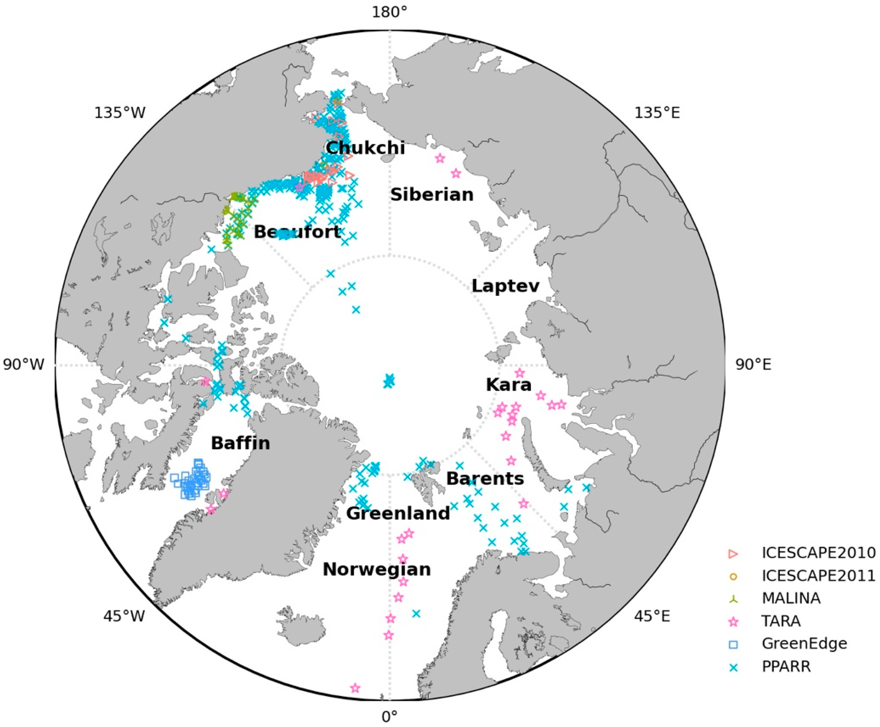
Data collected through PPARR (Primary Production Algorithm Round-Robin) was used for comparison purposes with the satellite climatology products only. In short, at each station, surface Chl was measured via the fluorometric method at depths between 0 and 5 m, while PP was measured at various depths using 13C- or 14C-labeled compounds. Details are described at [38]. The numbers of stations, sampling dates, sampling regions and data source from all expeditions are summarized in Table 1, while the locations of sampling stations are shown in Figure 1.

Table 1.
Summary of in situ datasets.
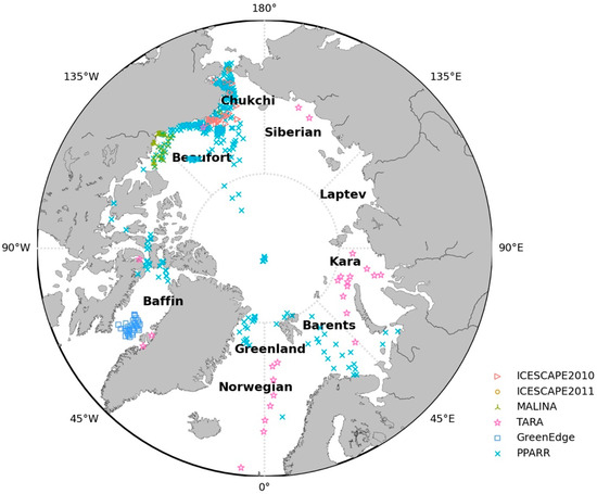
Figure 1.
Map of the Arctic Ocean showing the locations of stations from various datasets.
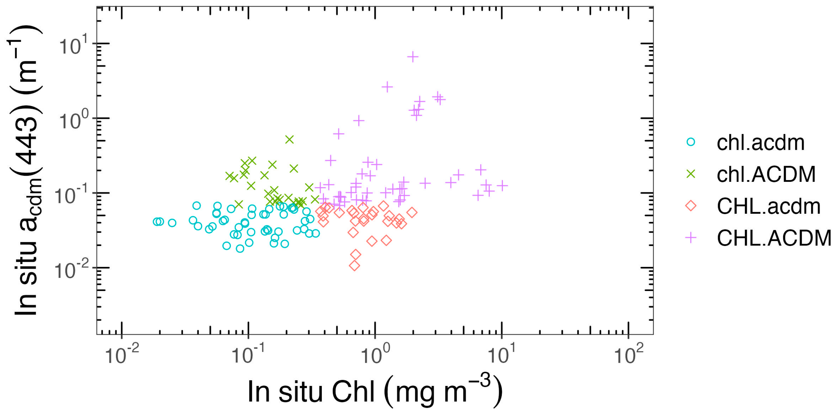
To evaluate algorithms from the perspective of the impact of CDM, we arbitrarily split the algorithm-evaluation dataset into 4 water types. For this purpose, missing values were estimated according to [39]. Then, based on the measured median value of Chl (0.35 mg m−3), we split the in situ dataset in half. For the half with Chl 0.35 mg m−3, samples with 0.067 m−1 were classified as chl.acdm, while those with > 0.067 m−1 were regarded as chl.ACDM. The same procedure was applied to the other half of the dataset with Chl > 0.35 mg m−3, thus deriving CHL.acdm and CHL.ACDM. This classification approach is illustrated in Figure 2 and Table 2.
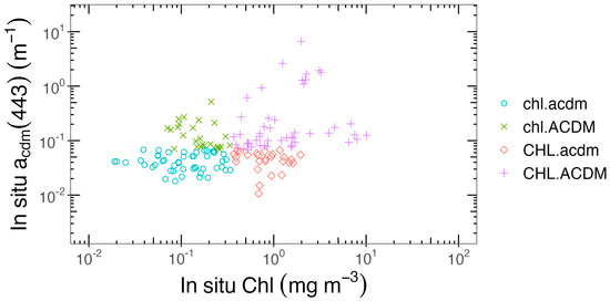
Figure 2.
This scatter plot illustrates water-type classification according to the level of and Chl in the water column.
Table 2.
Classification criteria.
2.2. Satellite Products
OC-CCI (Ocean Color Climate Change Initiative, https://esa-oceancolour-cci.org/, accessed on 12 August 2020) L3b daily chlorophyll products and reflectance products and MODIS atmospheric products (MYD08, https://ladsweb.modaps.eosdis.nasa.gov, accessed on 20 August 2020) in August from 2003 to 2018 were downloaded to generate climatology Chl and PP products for the AO. Note that the OC-CCI chlorophyll products were merged products based on SeaWiFS (Sea-viewing Wide Field-of-view Sensor), MERIS (Medium Resolution Imaging Spectrometer), aqua-MODIS (Moderate Resolution Imaging Spectroradiometer) and VIIRS (Visible Infrared Imaging Radiometer Suite) data to obtain as many pixels as possible, and Chl values were calculated using blending algorithms based on the water types, as documented in ATBD–OCAB (Algorithm Theoretical Baseline Document–Ocean Color Algorithm Blending, [40]), which is substantially an empirical approach.
2.3. Descriptions of Existing Operational Ocean-Color Algorithms
In this study, global empirical algorithms for SeaWiFS (OC4v6), MODIS (OC3Mv6), VIIRS (OC3V), two regional empirical algorithms (OC4L and OC4P), one AO empirical algorithm AO.emp and two semi-analytical algorithms (GSM01 and GSM.AO) were evaluated.
2.3.1. Empirical Algorithms
All empirical algorithms use polynomial functions to fit the relationship between Chl and the maximum blue-to-green ratio of remote-sensing reflectance:
where is the base-10 logarithm of the maximum blue-to-green band ratio of and are empirically derived coefficients listed in Table 3.
Table 3.
Band configurations and coefficients of the empirical chlorophyll a algorithms evaluated.
Note that wavelengths used for the blue and green bands vary slightly among sensors (see Table 3) and they were designed for different water bodies. OC3Mv6, OC4v6 and OC3V were obtained using a global in situ dataset, mainly from Case 1 and non-polar waters [23,24]. OC4P and OC4L were tuned using in situ measurements made in Canadian Arctic waters (in the vicinity of Resolute Bay and in the Labrador Sea [25]) and the Western Arctic (Chukchi and Beaufort Seas [21]), respectively. AO.emp was optimized using a large dataset compiled at a pan-Arctic scale [20,41].
2.3.2. Semi-Analytical Algorithm—GSM
The GSM semi-analytical ocean-color model was initially developed by [42] and later updated by [26] for SeaWiFS over non-polar Case 1 waters. The basic principle is to minimize the difference between the measured and modeled below-surface remote-sensing reflectance using non-linear optimization until a predefined convergence threshold is met. A detailed description of the GSM01 model and values of model parameters can be found in [26].
The GSM model can be tuned easily by reparameterizing model parameters using bio-optical data. The authors in [20] optimized the model parameters using a genetic optimization method for the AO based on the Arctic dataset described in [41], and the tuned model was named AO.GSM. They found that the optimized parameters more accurately represent the AO’s unique bio-optical characteristics. Details of the genetic optimization procedure and parameter values were described in [20].
2.4. Evaluation Criteria
The performance of each ocean-color algorithm was assessed following the metrics described in [43]. The first is the number of effective retrievals, . For example, GSM01 may generate negative Chl values due to the optimization regime; these negative retrievals were considered as failures. The next two metrics are bias and mean absolute error (MAE), which have been proven to be robust and straightforward metrics for evaluating ocean-color algorithms with non-Gaussian distributions and outliers [43].
Bias illustrates the systematic direction of error, as either underestimation or overestimation on average. A bias close to 1 means minimum bias, while a value lower than 1 reflects underestimation. A bias of 0.8, for instance, reflects 20% underestimation. The same reasoning holds for overestimations. MAE indicates random error and is always larger than 1. For instance, an MAE of 1.2 means an average of 20% relative error in retrievals compared to measured values.
The fourth metric is wins, which is obtained through pairwise comparison. That is, for each pair of estimated and measured variables, residuals (defined as estimated value minus measured value) for model A and model B are calculated, and the model with the lower residual is the winner, while models that fail are directly designated as losers. Wins, described as the percentage of winners to the total number of pairs, can be used to tell which model performs better and help to decide which model should be used in applications.
In addition, the slope and coefficient of determination () for log-transformed variables were also produced via type II reduced major axis (RMA) regression [44] as complementary metrics.
2.5. Primary-Production Model
The spectrally resolved primary-production model for the Arctic waters developed by [18] was adopted in the present study. One advantage of this model compared to others [17,45,46] is its consideration of the propagation of spectral light in the atmosphere and the ocean, using methods appropriate for both Case 1 and Case 2 waters. In recent years, this model has been further optimized to account for subsurface chlorophyll maxima often observed in the AO. This was achieved using the statistical relationships between Chl at surface and at depth, published by [47]. Furthermore, instead of using and Chl data from the GlobColour dataset as in [18], the present study used -merged products based on SeaWiFS, MERIS, aqua-MODIS and VIIRS data from OC-CCI for better coverage and derived Chl products through the merged products using the above-mentioned chlorophyll algorithms.
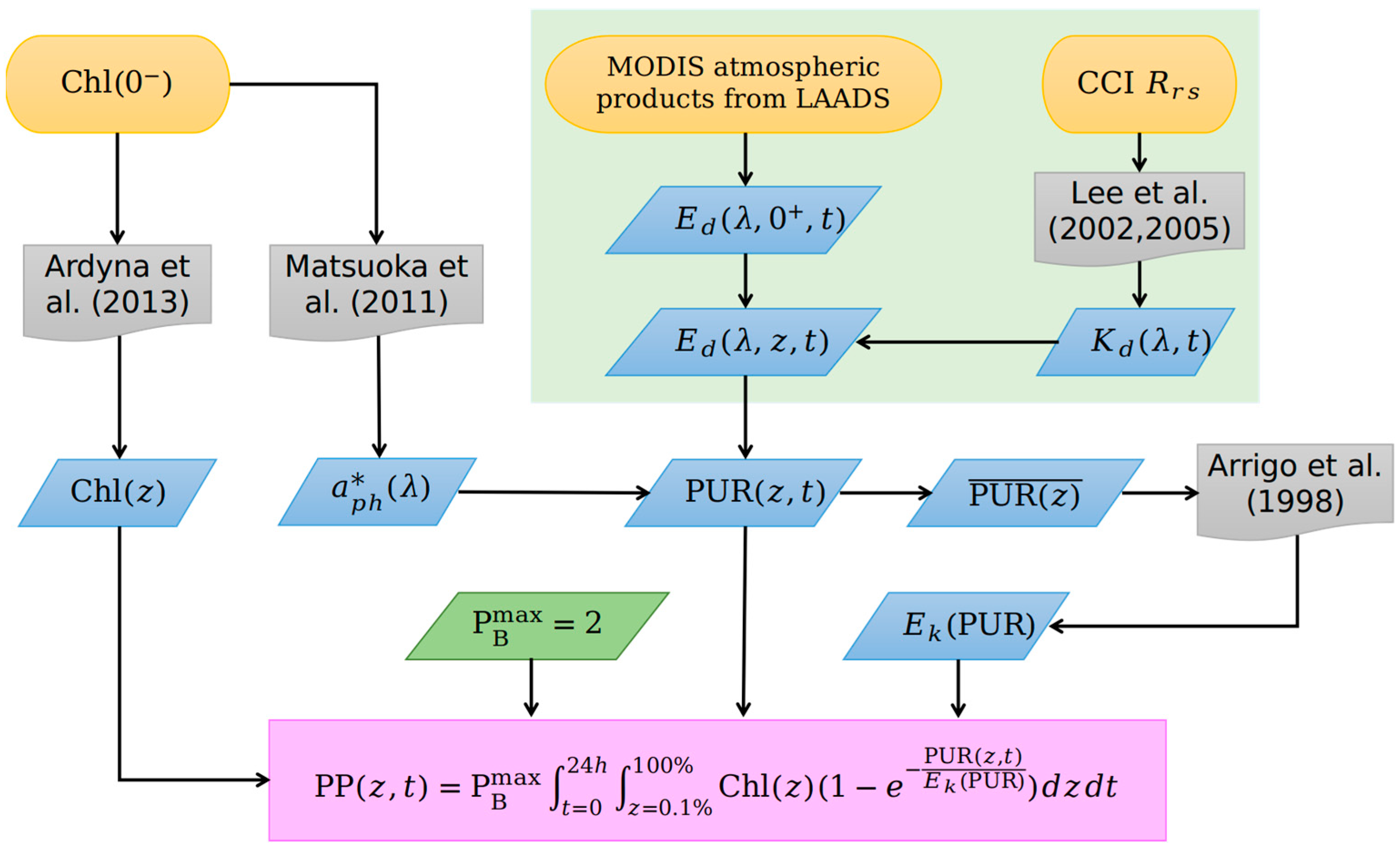
The structure of this spectrally and vertically resolved Arctic primary-production model is illustrated in Figure 3. Basically, the daily rates of carbon fixation by phytoplankton cells in units of mgC m−2 d−1 are estimated using the classical photosynthesis versus light model [48]:
where (mgC mgChl−1 h−1) is the light-saturated chlorophyll-normalized carbon-fixation rate, which is assumed as being constant at 2.0 mgC mgChl−1 h−1 (see [18] and references therein). Chl(z) is chlorophyll concentration at a given depth , which can be propagated from surface values following [47]. is the photosynthetically usable radiation expressed in µmol photons m−2 s−1 [49], which can be estimated using input atmospheric data and satellite-observed , and the spectral model of light propagation through the atmosphere and ocean has been described in [18]. (µmol photons m−2 s−1) is the saturation irradiance, parameterized here as a function of PUR [18].
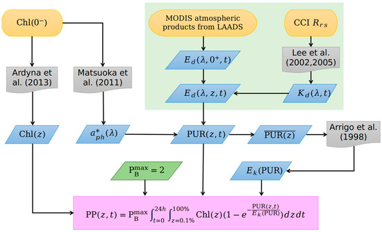
Figure 3.
Structure of the spectrally and vertically resolved Arctic primary-production model. Yellow, gray, blue, green and magenta frames refer to model inputs, methods described in the literature, intermediate variables, constant values and photosynthesis models, respectively (courtesy of Marcel Babin and Simon Bélanger) [47,50,51,52,53].
To quantify the impact of Chl retrievals derived from various algorithms on PP estimates, we performed a sensitivity analysis using an Arctic primary-production model, as described below. In short, measured Chl and , along with the temporally and geographically matched atmospheric parameters, were inputted into the Arctic primary-production model to derive spectrally and vertically resolved PP (named as PP-Ref). Subsequently, the Chl input alone was replaced by the Chl estimates derived through the various above-mentioned chlorophyll algorithms, using measured to obtain PP estimates (named as PP-Algorithm; for instance, PP generated via OC4L-derived Chl was referred to as PP-OC4L). Note that, since the primary-product model is a bin-based approach, several samples might be projected to the same bin; therefore, the total number of PP estimates is 135 rather than 148. Also note that, in this model, PP is not exactly proportional to Chl (Figure 3).
2.6. Climatology Products
Chl climatology product in August was obtained by averaging all the OC-CCI daily Chl products collected in August from 2003 to 2018. Meanwhile, to obtain the PP climatology product in August, firstly, each daily Chl product acquired in August was entered into the Arctic primary-production model (described in Section 2.4) along with corresponding daily reflectance product and MODIS atmospheric product to derive the daily PP product; then, all the daily PP products were averaged to calculate the climatology PP product.
2.7. Matchup Analysis
The algorithm-evaluation dataset was first matched with PPARR to search for concurrent measurements of both Chl and PP. This in situ dataset was then compared with daily Chl and PP products (described in Section 2.6) to look for temporal- and spatial-matched pairs. Concretely, this meant, for each in situ entry, keeping only the closest (within 4 km) satellite data obtained on the same day. Finally, only 5 in situ and satellite matchups were thus identified due to the lack of in situ measurements in the AO.
3. Results
3.1. Overview of Product Performance
Given the lack of in situ and satellite matchups, the accuracy of Chl products at a pan-Arctic scale was generally assessed by comparing the climatology Chl product in August (Figure 4a) with the in situ Chl measurements taken in August from PPARR via a kernel density plot (Figure 4b). It was found that the Chl product tends to generate higher estimates (median Chl = 0.66 mg m−3) compared with the in situ values (median Chl = 0.40 mg m−3), especially in the section where Chl < 1.2 mg m−3 (accounting for nearly 2/3 of all pixels). This comparison also yielded a small percentage of visibly higher estimates in the 4.0 to 11.0 mg m−3 range. By referring to the Chl distribution shown in Figure 4a, we can see that this proportion of higher estimates can be attributed to areas in and around the large river plumes, which hold considerable amounts of CDM as a result of river discharge.
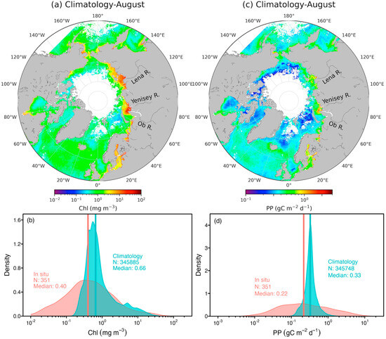
Figure 4.
(a) Climatology chlorophyll product in August derived through the blended empirical algorithm; (b) kernel density plot of Chl measurements collected in August from PPARR (red) and Chl climatology product in August (green); (c) climatology primary product in August produced through the Arctic primary-production model using OC-CCI daily reflectance and chlorophyll products; (d) kernel density plot of PP measurements collected in August from PPARR (red) and PP climatology product in August (green).
The corresponding climatology PP product is shown in Figure 4c, and the density curve compared with PP measurements from PPARR (same pairs of Chl measurements shown in Figure 4b) is illustrated in Figure 4d. As in the case of Chl estimates, PP estimates were also higher overall (median PP = 0.33 gC m−2d−1) in comparison with in situ values (median PP = 0.22 gC m−2d−1). Only one crest was recorded, located at 0.33 gC m−2d−1. One-third of all the PP estimates in the 0.007 to 0.2 gC m−2d−1 range were higher than the measurements, which is likely due to the higher Chl estimates. In the higher range PP > 0.6 gC m−2d−1, another one-third of PP estimates were lower than measurements. The higher estimates on the left side and lower estimates on the right side steepened the crest, resulting in the density at the crest being nearly 8 times that of the in situ one. Significantly, the higher Chl estimates in and around the large river plumes did not lead to higher PP estimates. It is likely that the high proportion of CDM in the water column was extremely absorbent of sunlight, thereby resulting in less PUR for absorption by phytoplankton [54].
3.2. Bio-Optical Algorithm Evaluations
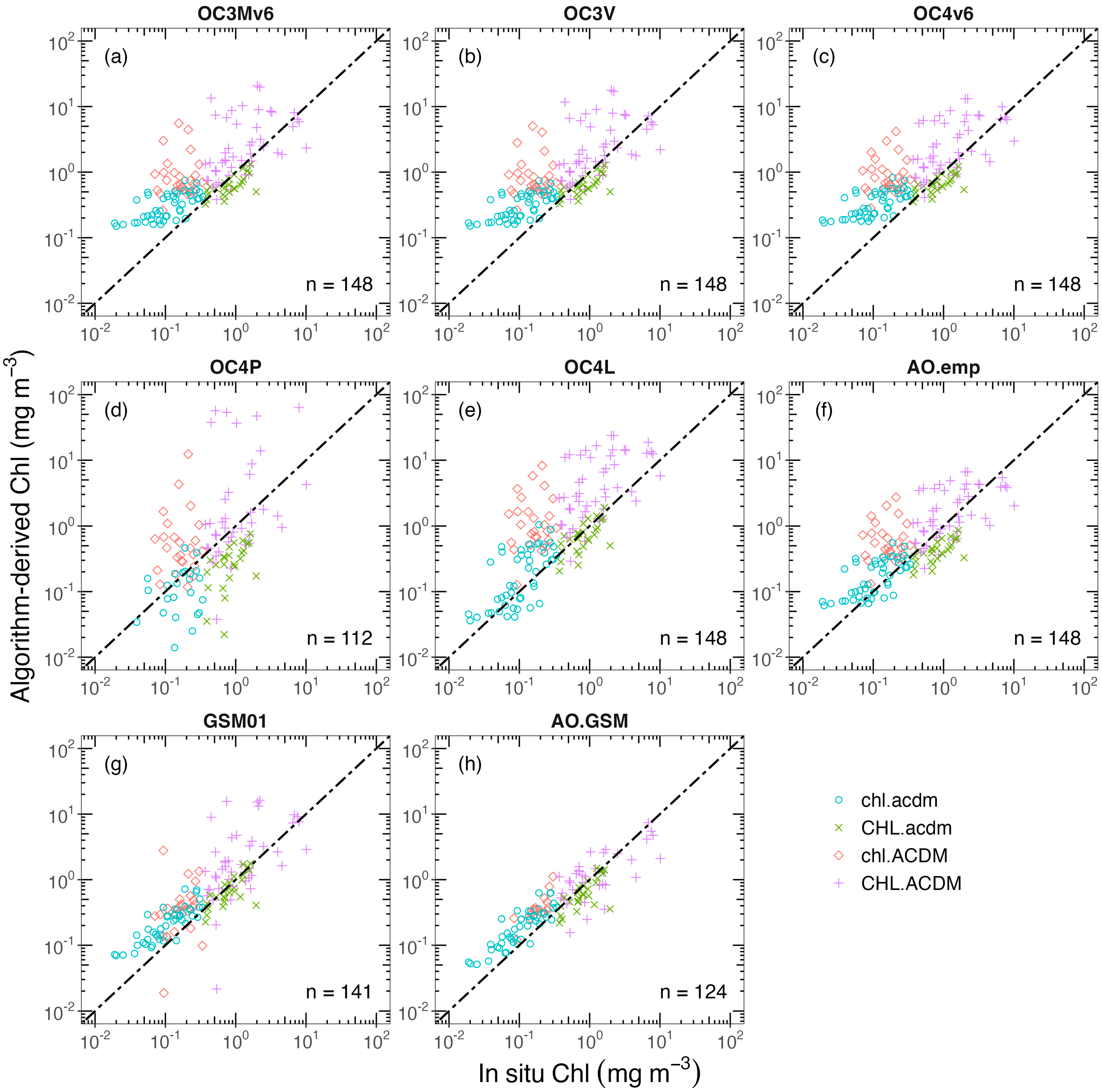
Chl is one of the key variables that influences PP estimates [18]. Because several chlorophyll algorithms are available, their relative performance needs to be examined first. Figure 5 shows the comparison between measured and estimated Chl using the various algorithms mentioned above for the four water types (see definition in Section 2.3). Overall, all the algorithms showed a trend of overestimation. OC4v6 and OC4L boosted estimations the most, overestimating by 132%, whereas OC4P was the least biased but had the largest MAE (Table 4). The MAE of AO.GSM was the smallest, followed by GSM01, AO.emp and, lastly, by the three global algorithms. The MAE of OC4L was noticeably larger than that of the global algorithms, indicating that regional Arctic empirical algorithm was not suitable for the pan-Arctic Ocean, as regional algorithms are subject to the compatibility of the waters under study with the waters from which data were obtained for algorithm development. As for the performance of regression, AO.GSM had the largest , but its slope was not as close to 1 as those of the other algorithms, except the two Arctic regional algorithms OC4P and OC4L.
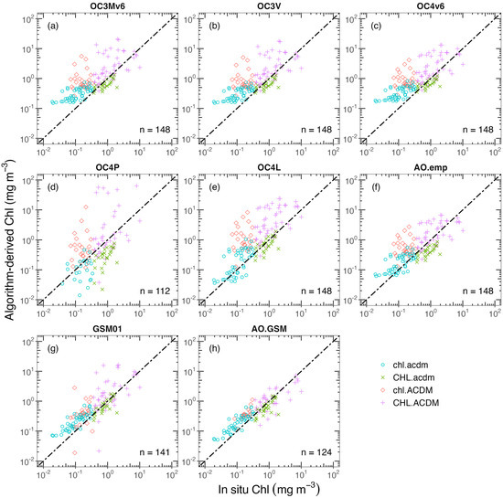
Figure 5.
Comparisons between measured and estimated Chl using (a) OC3Mv6, (b) OC3V, (c) OC4v6, (d) OC4P, (e) OC4L, (f) AO.emp, (g) GSM01, and (h) AO.GSM in 4 water types (see Table 2 for definition).
Table 4.
Performance metrics of the various algorithms evaluated.
To rank the overall performances of all the algorithms tested, percentage wins between every pair combination of two algorithms were calculated (Table 5). Among the three global algorithms, OC3Mv6 performed the best and OC4v6 was the worst. They all outperformed the two regional Arctic algorithms, but lost when compared with AO.emp, GSM01 and AO.GSM. OC4L only performed better than OC4P, which had the worst performance among all. As for GSM01, it outperformed the other algorithms except AO.emp and AO.GSM. The percentage wins of AO.emp were equal to those of AO.GSM. However, AO.emp emerged with a larger proportion of overall wins (65.6%). In this way, AO.emp was the best algorithm among all tested in the present study.
Table 5.
Algorithm performance assessed through pair-to-pair comparison.
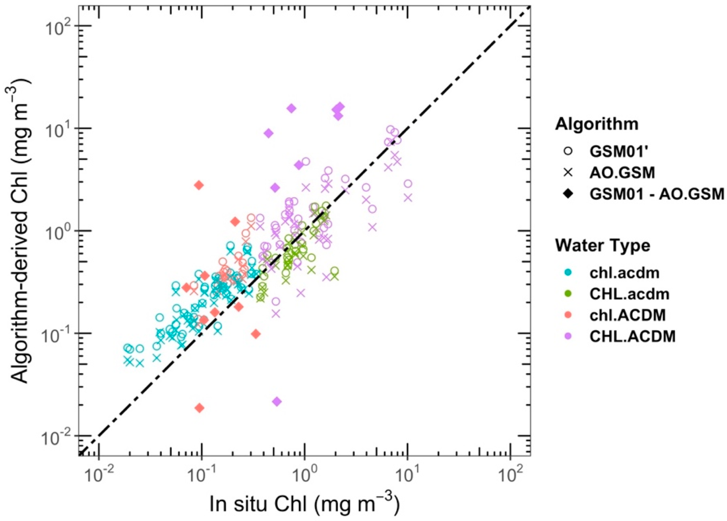
When taking a closer look at the different water types, symbols representing waters with high CDM (i.e., ‘diamonds’ for chl.ACDM and ‘pluses’ for CHL.ACDM) are distributed in a more scattered fashion than those for waters with low CDM for all empirical algorithms and GSM01 (Figure 5). However, this phenomenon is not visible for AO.GSM because, for waters with high CDM, this algorithm obtained 24 failures (accounting for 16.2% of the total sample), which were excluded from comparisons (see Figure 6 and Table 6). In other words, AO.GSM is more likely to fail for waters with high CDM. These findings indicate that the high proportion of CDM in the water column is the main obstacle for the success of these empirical and semi-analytical algorithms.

Figure 6.
Pair-to-pair comparison between GSM01 and AO.GSM; circles and x symbols refer to the same data pairs derived from GSM01 and AO.GSM, and diamonds refer to the data failed using AO.GSM but succeeding using GSM01.
Table 6.
Performance metrics of GSM01 and AO.GSM by individual water type and across all water types.
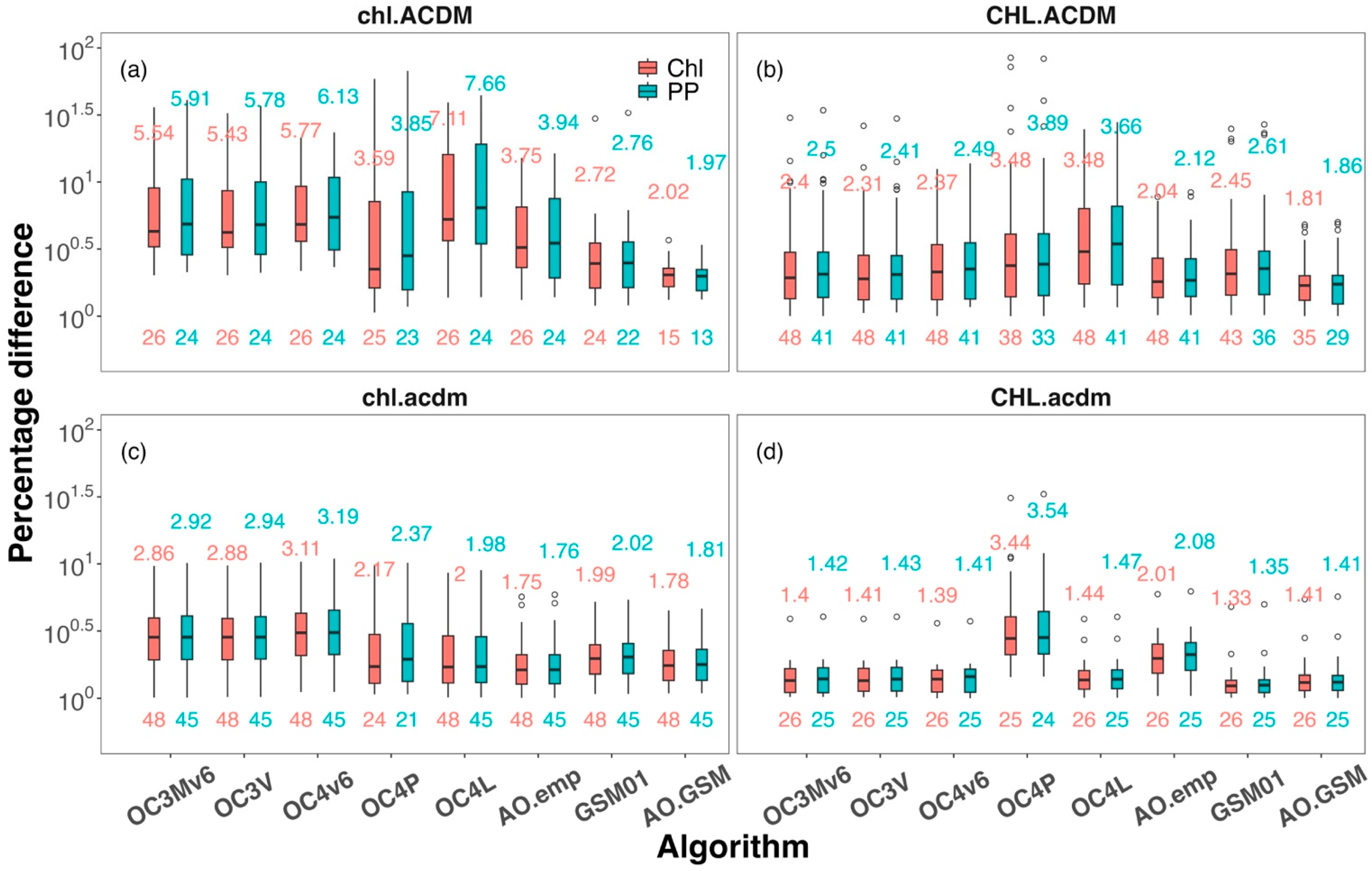
Boxplots were deployed to quantify the difference between measured and estimated Chl by individual algorithms for each water type (Figure 7). The MAEs were also labeled. Generally, the MAE of most of the algorithms tested (except OC4P and AO.emp) was the smallest for CHL.acdm (1.33 to 1.44), but the largest for chl.ACDM (2.02 to 7.11). Combined with the finding that the MAE for chl.acdm was smaller than that for CHL.ACDM, our results suggest that, the higher the level of CDM in relation to Chl, the greater the uncertainties surrounding Chl estimates. Given that OC4P had the largest MAE (3.16) and most failures (24.3%), it is hereafter excluded from further analysis.
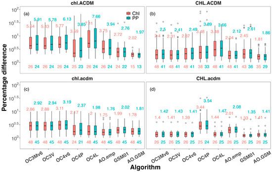
Figure 7.
Boxplots of percentage difference between measured and estimated Chl (red), between PP derived using measured Chl and PP estimated from algorithm-derived Chl (green) for water type (a) chl.ACDM, (b) CHL.ACDM, (c) chl.acdm, and (d) CHL.acdm (see Table 2 for definition). The labels above boxplots show MAE; those below show the numbers of samples classified as a certain water type.
For waters with low CDM (waters where < 0.067 m−1 in this study), the three global algorithms had the highest MAE, with values up to 2.86, followed by OC4L, GSM01 and AO.GSM for chl.acdm (Figure 7). AO.emp obtained the lowest MAE (1.75) but obtained the largest MAE (2.01) for CHL.acdm, as confirmed by the notable underestimation shown by the ‘x’ symbols in Figure 5. The MAEs of the other algorithms were around only 1.4 for CHL.acdm, with GSM01 producing the smallest (1.33).
For waters with high CDM (i.e., chl.ACDM and CHL.ACDM), OC4L obtained the largest MAEs (7.11 and 3.48, respectively), indicating that this regional Arctic empirical algorithm is less applicable for CDM-rich waters than the global empirical algorithms. AO.emp yielded the smallest MAE among all empirical algorithms tested for waters with high CDM, but the contrary was found for CHL.acdm. It seems that empirical algorithms only consider the main characteristics of water bodies and, thus, cannot work well for all types of waters. However, the two GSM models had the smallest MAEs for chl.ACDM and obtained relatively good performances for other water types. It is therefore recommended that semi-analytical algorithms, such as GSM-like models, be used for CDM-rich waters, even if they might produce failures.
To give a comprehensive comparison of the two GSM models, Table 6 summarizes the performance metrics for each water type. According to the wins, AO.GSM outperformed GSM01 for chl.acdm and chl.ACDM, but lost for CHL.acdm and CHL.ACDM. Figure 6 shows the pair-to-pair comparisons, with the diamond symbols representing the samples which failed with AO.GSM but succeeded with GSM01. The latter all belonged to water types with high CDM, and most of them were located far from the 1:1 regression line. When excluding these diamonds, AO.GSM outperformed GSM01, with 71.0% wins (see Table 6). It was thus shown that AO.GSM has the ability to eliminate retrievals with poor performance.
In terms of overall wins, AO.emp was the best chlorophyll algorithm tested. However, for waters with high CDM, which are of particular interest here, GSM-like models demonstrate better performance for the AO than empirical algorithms.
3.3. Impacts on PP Estimates
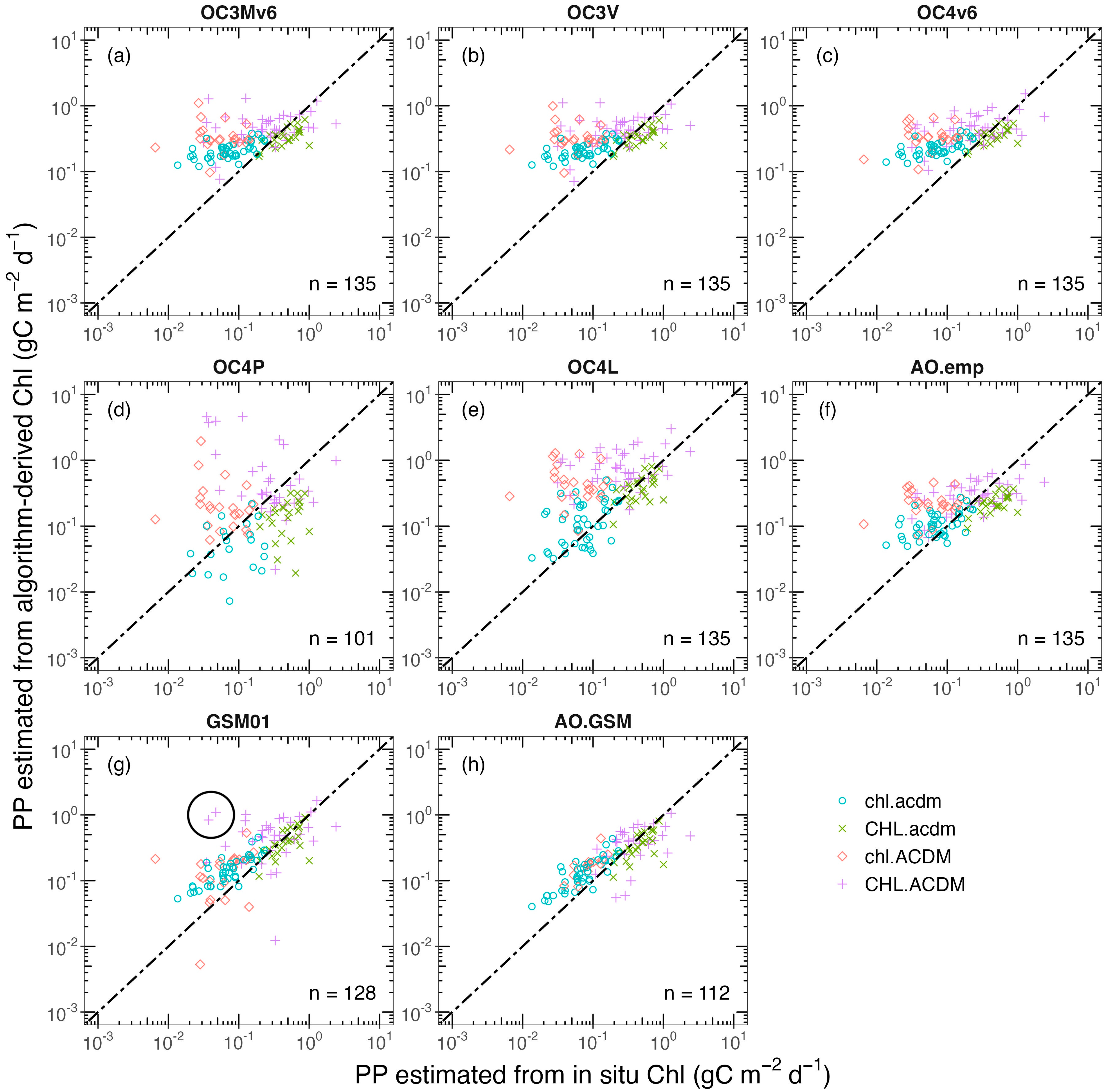
Figure 8 shows the comparisons between PP-Ref and each PP-Algorithm (see Section 3.3 for definition). Generally, the comparisons of PP estimates followed the same trends as those for Chl. In other words, when Chl was overestimated, the corresponding PP-Algorithm also showed a trend of overestimation compared with PP-Ref. The same was also true for underestimation. It should be noted that the boundaries between water types grew blurry with respect to Chl level. For instance, some ‘plus’ symbols (see the black circle in Figure 8) representing water type CHL.ACDM were located to the left of some ‘circle’ and ‘diamond’ symbols that referred to waters with low Chl, indicating that PP for waters with low surface Chl can exceed that with high surface Chl due to the possible existence of a prominent subsurface chlorophyll maximum.
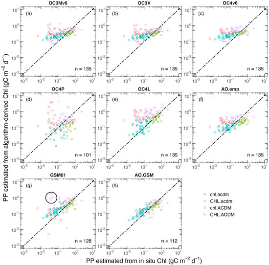
Figure 8.
Comparisons between PP estimated from in situ Chl and PP estimated from (a) OC3Mv6, (b) OC3V, (c) OC4v6, (d) OC4P, (e) OC4L, (f) AO.emp, (g) GSM01, and (h) AO.GSM-derived Chl for 4 water types (see Table 2 for definition). The black circle in subfigure (g) is used to illustrate the mix of water types in terms of the level of Chl in the water column.
The same boxplots of percentage difference between PP-Ref and PP-Algorithm are shown in Figure 6. It can be seen that the percentage differences of PP followed the trends of Chl, and the rankings of MAE reflected those of Chl but with relative larger values. Taking the best algorithm AO.emp as an example, the MAEs of PP were 0.5%, 3.4%, 5.1% and 3.9% larger than those of Chl for water types chl.acdm, CHL.acdm, chl.ACDM and CHL.ACDM, respectively. In addition, the amplifications of difference from Chl to PP were generally greater in waters with a relatively high proportion of CDM. Overall, considering all the algorithms, the amplification of difference from Chl to PP, largely due to the statistical approximation of the vertical Chl profile, did not exceed 7%.
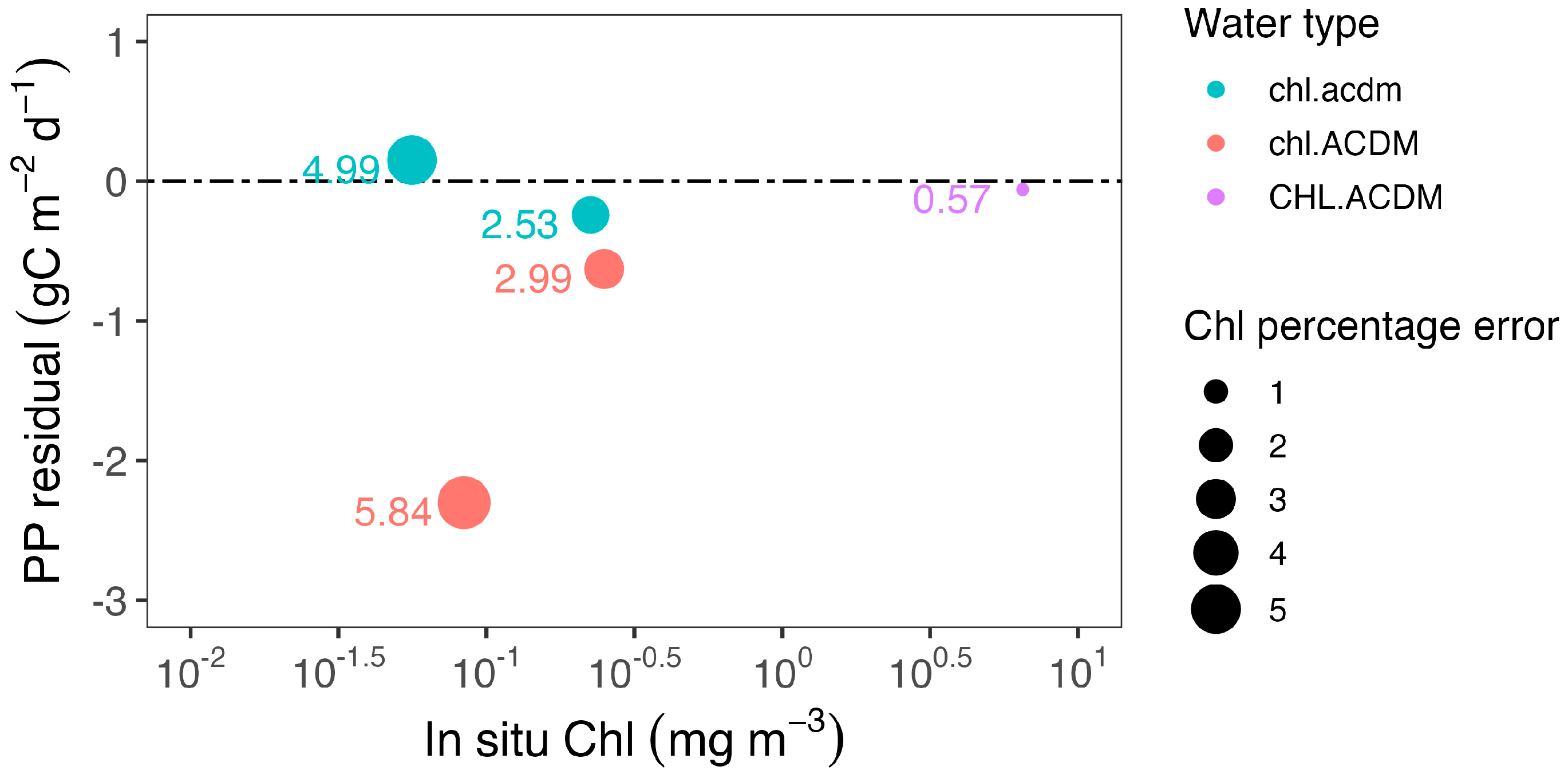
In addition to the assessment of how error in Chl estimates would impact PP estimates, the influence of CDM on PP estimates was also explored through in situ and satellite analysis. Figure 9 shows the residual of PP estimates resulting from Chl errors for waters with different levels of CDM. For waters with comparable levels of Chl and CDM (i.e., water types chl.acdm and CHL.ACDM), PP absolute errors vary from 0.06 to 0.24 gC m−2 d−1, which are lower values than for chl.ACDM. We can also note that a 399% overestimation of Chl (see the upper green symbol in Figure 9) merely led to 0.15 gC m−2 d−1 absolute error in PP for waters with low CDM, whereas, for waters with high CDM, a lower overestimation (199%) of Chl could result in a higher absolute error (0.62 gC m−2 d−1). Meanwhile, a 484% overestimation of Chl induced an absolute error that reached 2.3 gC m−2 d−1 in PP. In this way, a high CDM level (relative to Chl) in the water column may not only cause a larger error in the inversion of Chl, but may also lead to a larger absolute error in the estimation of PP. In addition, the Arctic primary-production model used in this study generally showed a trend of underestimation, especially for the water type chl.ACDM. However, more matchup analyses are needed to validate the Arctic primary-production model and quantify the errors.
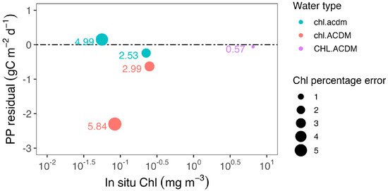
Figure 9.
Relationship between PP absolute error (PP estimated from in situ Chl subtracted from measured PP) and in situ Chl through matchup analyses. Labels refer to percentage errors of Chl estimates. A value of 4.99 means overestimation by 399%, while a value of 0.57 reflects 43% underestimation.
4. Discussions and Perspectives
4.1. Chl Retrieval Error
As far as the three global chlorophyll algorithms—OC3Mv6, OC3V and OC4v6—are concerned, the assumed relationship between and Chl is problematic for the AO because the absorption properties of the latter are fundamentally different from those of typical Case 1 waters. Many studies [6,7,8,39,55,56,57] have documented that the non-water absorption of the AO is dominated by CDOM, even at the primary phytoplankton absorption peak around 443 nm. In this way, the presence of CDOM at levels higher than the global mean will reduce the signal at blue wavelengths due to its strong absorption. As a consequence, global empirical algorithms using maximum blue-to-green ratios tend to have lower maximum band ratios, leading to an overestimation of Chl. Generally, the predominant influence of CDOM is to increase the intercept of the in situ versus algorithm-derived Chl regression and to only minimally change the slope [58].
In addition, due to the photo-acclimation of phytoplankton to low irradiance and cold temperature in the Arctic, an increase in phytoplankton cell size and/or in intra-cellular pigment concentration would decrease chlorophyll-specific absorption coefficient [6,8,21]. This higher package effect flattens the absorption spectrum of phytoplankton, especially at the blue absorption peak. Thus, in contrast to the effect of CDOM, a relatively larger decrease of at blue wavelengths than green wavelengths yields a larger maximum band ratio, leading to an underestimation of Chl when using global empirical algorithms for the AO. As a result, a relatively higher pigment-package effect decreases the slope of the in situ versus estimated Chl regression without significantly changing the intercept [58].
Overall, the difference between simulated and measured Chl is a consequence of combined effects of Chl overestimation due to relatively higher CDOM absorption and underestimation due to relatively higher pigment-package effects. In this study, the three global algorithms showed an obvious overestimation at all Chl ranges (Figure 5a–c), indicating that relatively higher CDOM absorption was the dominant factor that biased Chl estimates in the AO.
The failure of the two Arctic regional chlorophyll algorithms was imputed to the significant spatial variance of bio-optical properties at a pan-Arctic scale. The AO is a spatially heterogeneous sea. In other words, the composition of non-water constituents (i.e., phytoplankton, CDOM and NAP) and their bio-optical properties significantly differ from region to region due to varying degrees of river inputs, nutrient levels, sea ice coverage, shelf widths and circulation patterns [39,58]. Hence, a single regional empirical algorithm, like OC4L or OC4P, which are tuned for the Beaufort and Chukchi seas, is not appropriate for the entire AO. This is likely reflected by the worse performances that these algorithms recorded compared to the global empirical algorithms evaluated in the present study (see Figure 5 and Table 4). Such a degree of variability makes it difficult to establish a standard empirical formulation that may provide robust predictions with acceptable error limits, at least on the scale of the entire Arctic region. This was the case for AO.emp. Although the MAE of AO.emp was lower than those of the other algorithms for chl.acdm, for CHL.acdm, its MAE was even larger than those of the global algorithms. Thus, in theory, it is recommended to use a semi-analytical algorithm which compensates for optical properties in a given location through an optimization process and allows discrimination and quantification of the roles of non-phytoplankton constituents in the optical properties of seawater, to improve the accuracy of Chl estimates from OCRS in polar waters.
The standard semi-analytical algorithm GSM01, with parameters optimized for non-polar Case 1 waters, could not properly represent the combination of water constituents of the AO. In other words, due to the high CDM proportion in the AO, the spectral slope for should be sharper, and should be lower to account for higher package effect. This may be the reason why GSM01 performed worse than AO.emp (see Table 4). After reparameterization for the AO, AO.GSM outperformed GSM01 in the pair-wise comparison and showed the lowest MAEs for water types chl.ACDM and CHL.ACDM. However, for these two water types, AO.GSM also had 24 failures, which represents 16.2% of the total samples. Future research should, therefore, aim for a chlorophyll algorithm that can produce as many effective retrievals with reasonable uncertainty as possible.
4.2. PP Estimatation Error
The daily rates of carbon fixation, PP, by phytoplanktonic cells was estimated in the present study using a classical photosynthesis versus light model. The prime determinant of PP variations for ice-free waters in such models designed for OCRS data is Chl, except seasons when incident irradiance becomes highly limiting. It is expected that errors in Chl estimates propagate proportionally to PP, especially when all other variables are kept constant from one set of simulations to another, as in our study. In the model we used, however, Chl also drives the vertical distribution of Chl, as well as the chlorophyll-specific absorption coefficient of phytoplankton. Nevertheless, our results suggest and largely confirm that errors in Chl mostly propagate proportionally to PP.
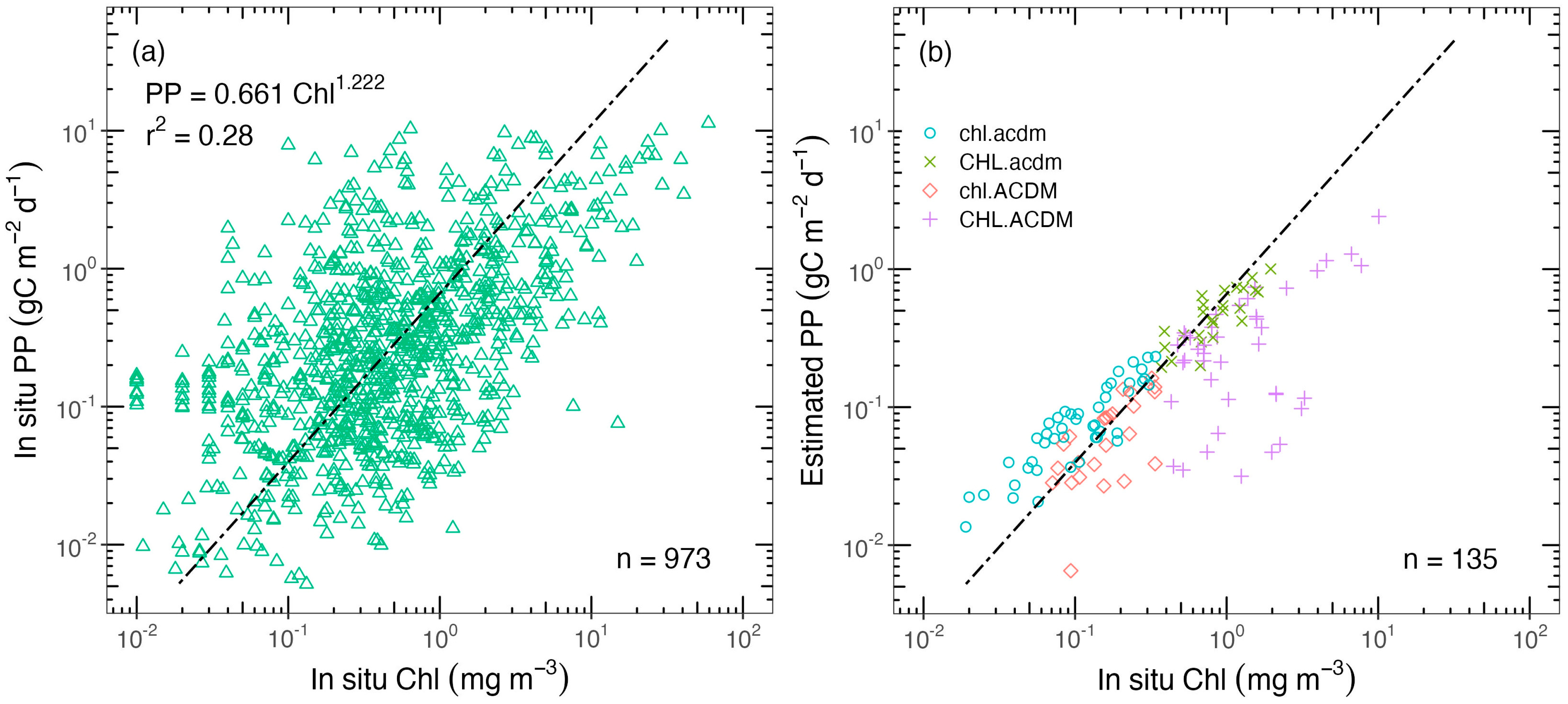
In the present study, since we only obtained five in situ and satellite-derived PP matchups, we further compared the PP estimates produced from the algorithm-evaluation dataset with the in situ PP from PPARR to assess their accuracy. Figure 10a shows the relationship between in situ PP and Chl using the PPARR dataset. It can be seen that, in the range of Chl from 0.1 to 1.0 mg m−3, PP varied across three orders, from 0.01 to 10.0 gC m−2 d−1. In addition, for Chl < 6.0 mg m−3, the triangle symbols were likely to be evenly distributed along the regression line, while, for Chl > 6.0 mg m−3, all triangles lay below the regression line. Figure 10b illustrates the relationship between estimated PP and measured Chl using the algorithm-evaluation dataset, duplicating the regression line of Figure 10a for the purpose of comparison. For waters with low CDM (i.e., water types chl.acdm and CHL.acdm), the estimated PP fitted the in situ regression line well. Meanwhile, for CDM-rich waters, PP estimates were more likely to be located at the bottom-right of the regression line, especially for CHL.ACDM, which was located the farthest from the regression line. It seems that chlorophyll-specific PP in CDM-rich waters is relatively lower than in waters with low CDM. In addition, various vertical Chl profiles with the same surface value may lead to significant variance in the estimation of PP. Therefore, remote-sensing detectable Chl vertical structures are still expected to obtain more accurate PP estimates in the future, and more in situ and satellite matchups are needed to quantify their accuracy.
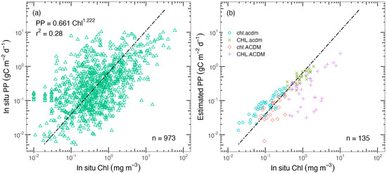
Figure 10.
(a) Relationship between in situ PP and Chl from PPARR; (b) relationship between PP estimates and in situ Chl using the dataset used for algorithm evaluation. The black dashed line is the regression line between in situ PP and Chl from PPARR.
5. Conclusions
Given that the poor performance of standard empirical algorithms in the AO is due to the interference by CDM in phytoplankton signals in the visible spectrum, in this study, we evaluated currently available algorithms to investigate the impact of CDM. We found that, the higher the level of CDM in relation to Chl in the water column, the larger the bias in the estimation of Chl. Overall, AO.emp performed the best among all the algorithms tested, but, for the CDM-rich waters that were of greatest interest here, GSM models performed better than all the empirical algorithms. Therefore, the use of an empirical algorithm for the entire AO should be avoided when possible. It is recommended that semi-analytical algorithms (such as GSM-like models) be used instead, as they can discriminate and quantify the roles of non-phytoplankton constituents for the heterogeneous AO. Nevertheless, given that AO.GSM is more likely to fail for waters with high CDM, future research is required to develop another semi-analytical algorithm that can produce as many effective retrievals with reasonable uncertainty as possible.
Through analysis of the sensitivity of PP estimations to Chl, we found that errors in Chl mostly propagated proportionally to PP and were slightly amplified (<7%), mainly due to the statistically vertically resolved Chl profile. In addition, matchup analysis allowed us to find that PP absolute error was much larger for CDM-rich waters. For instance, a 399% overestimation of Chl for waters with low CDM merely led to 0.15 gC m−2 d−1 absolute error in PP, while, for waters with high CDM, PP absolute error could reach up to 2.3 gC m−2 d−1, with an overestimation of Chl by 484%. It was also discovered that the spectrally and vertically resolved Arctic primary-production model used in this study underestimated PP to some extent. Overall, our PP calculations provide a quantitative indication of the uncertainty in PP estimates that should be expected in the Arctic for different seawater optical categories, as defined here.
Author Contributions
Conceptualization, M.B., A.M., X.P. and J.L.; methodology, M.B. and J.L.; software, J.L. and P.M.; validation, J.L.; formal analysis, J.L.; investigation, J.L.; resources, M.B. and A.M.; data curation, M.B., A.M. and J.L.; writing—original draft preparation, J.L.; writing—review and editing, M.B., A.M., X.P., P.M. and J.L.; visualization, J.L.; supervision, M.B., A.M. and X.P.; project administration, M.B.; funding acquisition, M.B., A.M. and X.P. All authors have read and agreed to the published version of the manuscript.
Funding
This research was funded by the Fundamental Research Funds for the Central Universities (2042023kf1044), the Sentinel North program of Université Laval (Canada First Research Excellence Fund), ArcticNet, SMAART, CNES (French space agency) and Marcel Babin’s NSERC Discovery Grant. Part of this research was supported by the National Aeronautics and Space Administration (NASA) Earth Science Division’s Interdisciplinary Science (sponsor award #1658689) and Japan Aerospace Exploration Agency (JAXA) Global Change Observation Mission-Climate projects (sponsor award #22RT000298 and #23RT000390) to Atsushi Matsuoka.
Data Availability Statement
The datasets used in this study can be found at MALINA [27], ICESCAPEs [28], TARA [29], GREEN EDGE [30] and PPARR [38].
Conflicts of Interest
The authors declare no conflicts of interest.
References
- Carmack, E.C.; Yamamoto-Kawai, M.; Haine, T.W.; Bacon, S.; Bluhm, B.A.; Lique, C.; Melling, H.; Polyakov, I.V.; Straneo, F.; Timmermans, M.-L.; et al. Freshwater and Its Role in the Arctic Marine System: Sources, Disposition, Storage, Export, and Physical and Biogeochemical Consequences in the Arctic and Global Oceans. J. Geophys. Res. Biogeosciences 2016, 121, 675–717. [Google Scholar] [CrossRef]
- Peterson, B.J.; Holmes, R.M.; McClelland, J.W.; Vörösmarty, C.J.; Lammers, R.B.; Shiklomanov, A.I.; Shiklomanov, I.A.; Rahmstorf, S. Increasing River Discharge to the Arctic Ocean. Science 2002, 298, 2171–2173. [Google Scholar] [CrossRef]
- Raymond, P.A.; McClelland, J.W.; Holmes, R.M.; Zhulidov, A.V.; Mull, K.; Peterson, B.J.; Striegl, R.G.; Aiken, G.R.; Gurtovaya, T.Y. Flux and Age of Dissolved Organic Carbon Exported to the Arctic Ocean: A Carbon Isotopic Study of the Five Largest Arctic Rivers: ARCTIC RIVER DOC. Glob. Biogeochem. Cycles 2007, 21. [Google Scholar] [CrossRef]
- Babin, M.; Arrigo, K.; Bélanger, S.; Forget, M.-H. Ocean Colour Remote Sensing in Polar Seas; International Ocean Colour Coordinating Group: Dartmouth, NS, Canada, 2015; Available online: https://ioccg.org/wp-content/uploads/2015/10/ioccg-report-16.pdf (accessed on 20 January 2018).
- Matsuoka, A.; Ortega-Retuerta, E.; Bricaud, A.; Arrigo, K.R.; Babin, M. Characteristics of Colored Dissolved Organic Matter (CDOM) in the Western Arctic Ocean: Relationships with Microbial Activities. Deep Sea Res. Part II Top. Stud. Oceanogr. 2015, 118, 44–52. [Google Scholar] [CrossRef]
- Stedmon, C.; Amon, R.; Rinehart, A.; Walker, S. The Supply and Characteristics of Colored Dissolved Organic Matter (CDOM) in the Arctic Ocean: Pan Arctic Trends and Differences. Mar. Chem. 2011, 124, 108–118. [Google Scholar] [CrossRef]
- Matsuoka, A.; Bricaud, A.; Benner, R.; Para, J.; Sempéré, R.; Prieur, L.; Bélanger, S.; Babin, M. Tracing the Transport of Colored Dissolved Organic Matter in Water Masses of the Southern Beaufort Sea: Relationship with Hydrographic Characteristics. Biogeosciences 2012, 9, 925–940. [Google Scholar] [CrossRef]
- Granskog, M.A.; Stedmon, C.A.; Dodd, P.A.; Amon, R.M.W.; Pavlov, A.K.; de Steur, L.; Hansen, E. Characteristics of Colored Dissolved Organic Matter (CDOM) in the Arctic Outflow in the Fram Strait: Assessing the Changes and Fate of Terrigenous CDOM in the Arctic Ocean. J. Geophys. Res. Ocean. 2012, 117. [Google Scholar] [CrossRef]
- Demidov, A.B.; Kopelevich, O.V.; Mosharov, S.A.; Sheberstov, S.V.; Vazyulya, S.V. Modelling Kara Sea Phytoplankton Primary Production: Development and Skill Assessment of Regional Algorithms. J. Sea Res. 2017, 125, 1–17. [Google Scholar] [CrossRef]
- Petrenko, D.; Pozdnyakov, D.; Johannessen, J.; Counillon, F.; Sychov, V. Satellite-Derived Multi-Year Trend in Primary Production in the Arctic Ocean. Int. J. Remote Sens. 2013, 34, 3903–3937. [Google Scholar] [CrossRef]
- Salyuk, P.A.; Stepochkin, I.E.; Bukin, O.A.; Sokolova, E.B.; Mayor, A.Y.; Shambarova, J.V.; Gorbushkin, A.R. Determination of the Chlorophyll a Concentration by MODIS-Aqua and VIIRS Satellite Radiometers in Eastern Arctic and Bering Sea. Izv. Atmos. Ocean. Phys. 2016, 52, 988–998. [Google Scholar] [CrossRef]
- Gonçalves-Araujo, R.; Rabe, B.; Peeken, I.; Bracher, A. High Colored Dissolved Organic Matter (CDOM) Absorption in Surface Waters of the Central-Eastern Arctic Ocean: Implications for Biogeochemistry and Ocean Color Algorithms. PLoS ONE 2018, 13, e0190838. [Google Scholar] [CrossRef]
- Vörösmarty, C.J.; Fekete, B.M.; Meybeck, M.; Lammers, R.B. Global System of Rivers: Its Role in Organizing Continental Land Mass and Defining Land-to-Ocean Linkages. Glob. Biogeochem. Cycles 2000, 14, 599–621. [Google Scholar] [CrossRef]
- Field, C.B.; Behrenfeld, M.J.; Randerson, J.T.; Falkowski, P. Primary Production of the Biosphere: Integrating Terrestrial and Oceanic Components. Science 1998, 281, 237–240. [Google Scholar] [CrossRef] [PubMed]
- Winder, M.; Sommer, U. Phytoplankton Response to a Changing Climate. Hydrobiologia 2012, 698, 5–16. [Google Scholar] [CrossRef]
- Cloern, J.E.; Foster, S.Q.; Kleckner, A.E. Phytoplankton Primary Production in the World’s Estuarine-Coastal Ecosystems. Biogeosciences 2014, 11, 2477–2501. [Google Scholar] [CrossRef]
- Arrigo, K.R.; van Dijken, G.; Pabi, S. Impact of a Shrinking Arctic Ice Cover on Marine Primary Production. Geophys. Res. Lett. 2008, 35, L19603. [Google Scholar] [CrossRef]
- Bélanger, S.; Babin, M.; Tremblay, J.-É. Increasing Cloudiness in Arctic Damps the Increase in Phytoplankton Primary Production Due to Sea Ice Receding. Biogeosciences 2013, 10, 4087–4101. [Google Scholar] [CrossRef]
- Kahru, M.; Brotas, V.; Manzano-Sarabia, M.; Mitchell, B.G. Are Phytoplankton Blooms Occurring Earlier in the Arctic? Glob. Chang. Biol. 2011, 17, 1733–1739. [Google Scholar] [CrossRef]
- Lewis, K.M.; Arrigo, K.R. Ocean Color Algorithms for Estimating Chlorophyll a, CDOM Absorption, and Particle Backscattering in the Arctic Ocean. J. Geophys. Res. Ocean. 2020, 125, e2019JC015706. [Google Scholar] [CrossRef]
- Cota, G.F.; Wang, J.; Comiso, J.C. Transformation of Global Satellite Chlorophyll Retrievals with a Regionally Tuned Algorithm. Remote Sens. Environ. 2004, 90, 373–377. [Google Scholar] [CrossRef]
- Bricaud, A.; Morel, A.; Prieur, L. Absorption by Dissolved Organic Matter of the Sea (Yellow Substance) in the UV and Visible Domains1. Limnol. Oceanogr. 1981, 26, 43–53. [Google Scholar] [CrossRef]
- O’Reilly, J.E.; Maritorena, S.; Mitchell, B.G.; Siegel, D.A.; Carder, K.L.; Garver, S.A.; Kahru, M.; McClain, C. Ocean Color Chlorophyll Algorithms for SeaWiFS. J. Geophys. Res. Ocean. 1998, 103, 24937–24953. [Google Scholar] [CrossRef]
- O’Reilly, J.E.; Maritorena, S.; Siegel, D.A.; O’Brien, M.C.; Toole, D.; Mitchell, B.G.; Kahru, M.; Chavez, F.P.; Strutton, P.; Cota, G.F.; et al. Ocean Color Chlorophyll a Algorithms for SeaWiFS, OC2 and OC4: Version 4. SeaWiFS Postlaunch Calibration Valid. Anal. 2000, 3, 9–23. [Google Scholar]
- Wang, J.; Cota, G.F. Remote-Sensing Reflectance in the Beaufort and Chukchi Seas: Observations and Models. Appl. Opt. 2003, 42, 2754. [Google Scholar] [CrossRef] [PubMed]
- Maritorena, S.; Siegel, D.A.; Peterson, A.R. Optimization of a Semianalytical Ocean Color Model for Global-Scale Applications. Appl. Opt. 2002, 41, 2705. [Google Scholar] [CrossRef]
- Massicotte, P.; Amon, R.M.W.; Antoine, D.; Archambault, P.; Balzano, S.; Bélanger, S.; Benner, R.; Boeuf, D.; Bricaud, A.; Bruyant, F.; et al. The MALINA Oceanographic Expedition: How Do Changes in Ice Cover, Permafrost and UV Radiation Impact Biodiversity and Biogeochemical Fluxes in the Arctic Ocean? Earth Syst. Sci. Data 2021, 13, 1561–1592. [Google Scholar] [CrossRef]
- Arrigo, K.R. Impacts of Climate on EcoSystems and Chemistry of the Arctic Pacific Environment (ICESCAPE). Deep Sea Res. Part II Top. Stud. Oceanogr. 2015, 118, 1–6. [Google Scholar] [CrossRef]
- Sunagawa, S.; Acinas, S.G.; Bork, P.; Bowler, C.; Eveillard, D.; Gorsky, G.; Guidi, L.; Iudicone, D.; Karsenti, E.; Lombard, F.; et al. Tara Oceans: Towards Global Ocean Ecosystems Biology. Nat. Rev. Microbiol. 2020, 18, 428–445. [Google Scholar] [CrossRef]
- Massicotte, P.; Amiraux, R.; Amyot, M.-P.; Archambault, P.; Ardyna, M.; Arnaud, L.; Artigue, L.; Aubry, C.; Ayotte, P.; Bécu, G.; et al. Green Edge Ice Camp Campaigns: Understanding the Processes Controlling the Under-Ice Arctic Phytoplankton Spring Bloom. Earth Syst. Sci. Data 2020, 12, 151–176. [Google Scholar] [CrossRef]
- Hooker, S.B.; Morrow, J.H.; Matsuoka, A. Apparent Optical Properties of the Canadian Beaufort Sea—Part 2: The 1% and 1 Cm Perspective in Deriving and Validating AOP Data Products. Biogeosciences 2013, 10, 4511–4527. [Google Scholar] [CrossRef]
- Antoine, D.; Hooker, S.; Bélanger, S.; Matsuoka, A.; Babin, M. Apparent Optical Properties of the Canadian Beaufort Sea—Part 1: Observational Overview and Water Column Relationships. Biogeosciences 2013, 10, 4493–4509. [Google Scholar] [CrossRef]
- Van Heukelem, L.; Thomas, C.S. Computer-Assisted High-Performance Liquid Chromatography Method Development with Applications to the Isolation and Analysis of Phytoplankton Pigments. J. Chromatogr. A 2001, 910, 31–49. [Google Scholar] [CrossRef]
- Ras, J.; Claustre, H.; Uitz, J. Spatial Variability of Phytoplankton Pigment Distributions in the Subtropical South Pacific Ocean: Comparison Between in Situ and Predicted Data. Biogeosciences 2008, 5, 353–369. [Google Scholar] [CrossRef]
- Hooker, S.B.; Zibordi, G. Platform Perturbations in Above-Water Radiometry. Appl. Opt. 2005, 44, 553. [Google Scholar] [CrossRef]
- Reynolds, R.A.; Stramski, D.; Neukermans, G. Optical Backscattering by Particles in Arctic Seawater and Relationships to Particle Mass Concentration, Size Distribution, and Bulk Composition: Particle Backscattering in Arctic Seawater. Limnol. Oceanogr. 2016, 61, 1869–1890. [Google Scholar] [CrossRef]
- Bricaud, A.; Babin, M.; Claustre, H.; Ras, J.; Tièche, F. Light Absorption Properties and Absorption Budget of Southeast Pacific Waters. J. Geophys. Res. 2010, 115, C08009. [Google Scholar] [CrossRef]
- Lee, Y.J.; Matrai, P.A.; Friedrichs, M.A.M.; Saba, V.S.; Ardyna, M.; Babin, M.; Gosselin, M.; Hirawake, T.; Kang, S.-H.; Lee, S.H. Water Temperature, Primary Productivity-Phytoplankton, Chlorophyll-a Concentration, and Other Data Collected by CTD, Scintillation Counter, Fluorometer, and Other Instruments from Arctic Ocean from 1959-08-03 to 2011-10-21 (NCEI Accession 0161176). 2018. Available online: https://catalog.data.gov/dataset/water-temperature-primary-productivity-phytoplankton-chlorophyll-a-concentration-and-other-data (accessed on 10 October 2020).
- Matsuoka, A.; Hooker, S.B.; Bricaud, A.; Gentili, B.; Babin, M. Estimating Absorption Coefficients of Colored Dissolved Organic Matter (CDOM) Using a Semi-Analytical Algorithm for Southern Beaufort Sea Waters: Application to Deriving Concentrations of Dissolved Organic Carbon from Space. Biogeosciences 2013, 10, 917–927. [Google Scholar] [CrossRef]
- Jackson, T.; Grant, M. Ocean Colour Climate Change Iniative (OC-CCI) Algorithm Theoretical Baseline Document (Ocean Colour Algorithm Blending). 2016. Available online: http://www.esa-oceancolour-cci.org/?q=webfm_send/587 (accessed on 19 December 2019).
- Lewis, K.; Van Dijken, G.; Arrigo, K. Bio-Optical Database of the Arctic Ocean. Dryad 2020. Available online: https://datadryad.org/stash/dataset/doi:10.5061/dryad.cnp5hqc17 (accessed on 10 October 2023).
- Garver, S.A.; Siegel, D.A. Inherent Optical Property Inversion of Ocean Color Spectra and Its Biogeochemical Interpretation: 1. Time Series from the Sargasso Sea. J. Geophys. Res. Ocean. 1997, 102, 18607–18625. [Google Scholar] [CrossRef]
- Seegers, B.N.; Stumpf, R.P.; Schaeffer, B.A.; Loftin, K.A.; Werdell, P.J. Performance Metrics for the Assessment of Satellite Data Products: An Ocean Color Case Study. Opt. Express 2018, 26, 7404. [Google Scholar] [CrossRef]
- Legendre, P. Model II Regression User’s Guide, r Edition. R Vignette 1998, 14. Available online: https://cran.r-project.org/web/packages/lmodel2/vignettes/mod2user.pdf (accessed on 2 April 2018).
- Pabi, S.; van Dijken, G.L.; Arrigo, K.R. Primary Production in the Arctic Ocean, 19982006. J. Geophys. Res. 2008, 113, C08005. [Google Scholar] [CrossRef]
- Perrette, M.; Yool, A.; Quartly, G.D.; Popova, E.E. Near-Ubiquity of Ice-Edge Blooms in the Arctic. Biogeosciences Discuss. 2010, 7, 8123–8142. [Google Scholar] [CrossRef]
- Ardyna, M.; Babin, M.; Gosselin, M.; Devred, E.; Bélanger, S.; Matsuoka, A.; Tremblay, J.-É. Parameterization of Vertical Chlorophyll a in the Arctic Ocean: Impact of the Subsurface Chlorophyll Maximum on Regional, Seasonal, and Annual Primary Production Estimates. Biogeosciences 2013, 10, 4383–4404. [Google Scholar] [CrossRef]
- Babin, M.; Bélanger, S.; Ellingsen, I.; Forest, A.; Le Fouest, V.; Lacour, T.; Ardyna, M.; Slagstad, D. Estimation of Primary Production in the Arctic Ocean Using Ocean Colour Remote Sensing and Coupled Physicalbiological Models: Strengths, Limitations and How They Compare. Prog. Oceanogr. 2015, 139, 197–220. [Google Scholar] [CrossRef]
- Morel, A. Available Usable and Stored Radiant Energy in Relation to Marine Photosynthesis. Deep Sea Res. 1978, 25, 673–688. [Google Scholar] [CrossRef]
- Lee, Z.; Carder, K.L.; Arnone, R.A. Deriving Inherent Optical Properties from Water Color: A Multiband Quasi-Analytical Algorithm for Optically Deep Waters. Appl. Opt. 2002, 41, 5755. [Google Scholar] [CrossRef]
- Lee, Z.-P.; Du, K.; Arnone, R. A Model for the Diffuse Attenuation Coefficient of Downwelling Irradiance. Estuar. Coast. Shelf Sci. 2005, 110, C02016. [Google Scholar] [CrossRef]
- Arrigo, K.R.; Worthen, D.; Schnell, A.; Lizotte, M.P. Primary Production in Southern Ocean Waters. J. Geophys. Res. Ocean. 1998, 103, 15587–15600. [Google Scholar]
- Matsuoka, A.; Hill, V.; Huot, Y.; Babin, M.; Bricaud, A. Seasonal Variability in the Light Absorption Properties of Western Arctic Waters: Parameterization of the Individual Components of Absorption for Ocean Color Applications. J. Geophys. Res. Ocean. 2011, 116. [Google Scholar] [CrossRef]
- Hessen, D.O.; Carroll, J.; Kjeldstad, B.; Korosov, A.A.; Pettersson, L.H.; Pozdnyakov, D.; Sørensen, K. Input of Organic Carbon as Determinant of Nutrient Fluxes, Light Climate and Productivity in the Ob and Yenisey Estuaries. Estuar. Coast. Shelf Sci. 2010, 88, 53–62. [Google Scholar] [CrossRef]
- Wang, J.; Cota, G.F.; Ruble, D.A. Absorption and Backscattering in the Beaufort and Chukchi Seas. J. Geophys. Res. 2005, 110, C04014. [Google Scholar] [CrossRef]
- Bélanger, S.; Babin, M.; Larouche, P. An Empirical Ocean Color Algorithm for Estimating the Contribution of Chromophoric Dissolved Organic Matter to Total Light Absorption in Optically Complex Waters. J. Geophys. Res. 2008, 113, C04027. [Google Scholar] [CrossRef]
- Mustapha, S.B.; Bélanger, S.; Larouche, P. Evaluation of Ocean Color Algorithms in the Southeastern Beaufort Sea, Canadian Arctic: New Parameterization Using SeaWiFS, MODIS, and MERIS Spectral Bands. Can. J. Remote Sens. 2012, 38, 535–556. [Google Scholar] [CrossRef]
- Lewis, K.M.; Mitchell, B.G.; van Dijken, G.L.; Arrigo, K.R. Regional Chlorophyll a Algorithms in the Arctic Ocean and Their Effect on Satellite-Derived Primary Production Estimates. Deep Sea Res. Part II Top. Stud. Oceanogr. 2016, 130, 14–27. [Google Scholar] [CrossRef]

Disclaimer/Publisher’s Note: The statements, opinions and data contained in all publications are solely those of the individual author(s) and contributor(s) and not of MDPI and/or the editor(s). MDPI and/or the editor(s) disclaim responsibility for any injury to people or property resulting from any ideas, methods, instructions or products referred to in the content. |
© 2024 by the authors. Licensee MDPI, Basel, Switzerland. This article is an open access article distributed under the terms and conditions of the Creative Commons Attribution (CC BY) license (https://creativecommons.org/licenses/by/4.0/).