
Ecosystem Integrity Remote Sensing—Modelling and Service Tool—ESIS/Imalys

 , , , , , and
Abstract
:1. Introduction
- (I)
- Presentation of the RS tool—ESIS/Imalys.
- (II)
- To present the RS indicators that can be derived based on the Imalys library.
- (III)
- Discuss the advantages and disadvantages of the new tool.
- (IV)
- Demonstrate the applicability of the RS-based indicators by means of several ecological applications.
- (V)
- Provide an overview of the technical background of the implementation of the Imalys library, data formats and possible graphical user interfaces.
2. The ESIS/Imalys Tool for Integrated Landscape Analysis with RS Data
2.1. The Aims of ESIS/Imalys Tool
2.2. Technological Foundations of the ESIS/Imalys Tool
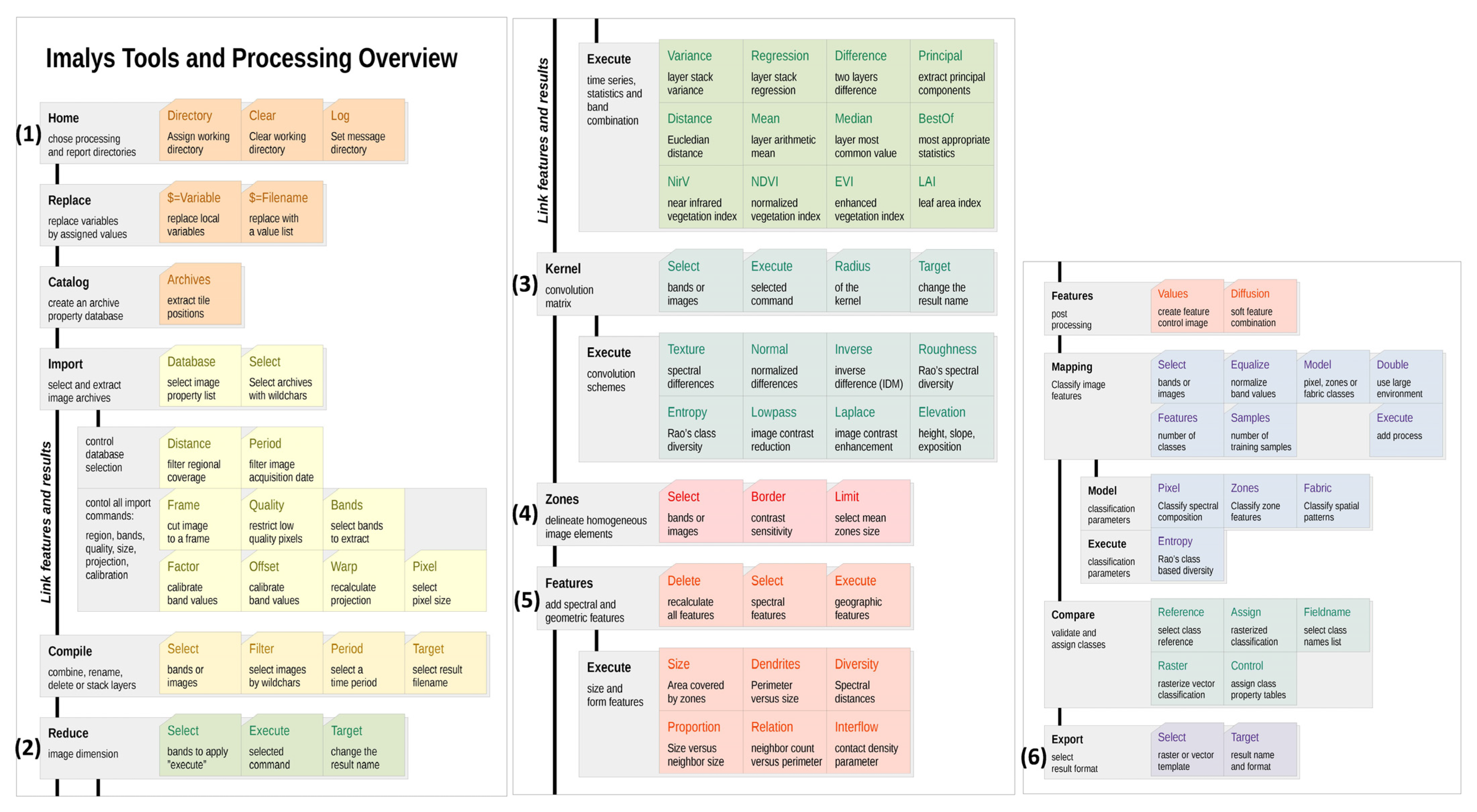
2.3. ESIS/Imalys Tool and Processing Overview
- Figure 2 (I) Data import and processing: The process selects spatially and temporally suitable RS data from any collection of provider archives (e.g., Google Earth Engine), checks the image quality within the given frame, extracts the selected bands from the archives, calibrates the raw data for TOA reflectance, reprojects all sections if necessary, combines sections from different tiles of the provider, generates a short time series and forms a data product with the most frequent values for each pixel for the selected period (see also Figure A1 (Appendix B) and Table A1 (Appendix B)).
- Figure 2 (II) Statistical reduction of RS data: Here, the user can find methods for the statistical reduction of large RS datasets such as Mean, Median, Principal and Replace Image Bands (see also Figure A1 (Appendix B) and Table A1 (Appendix B)).
- Figure 2 (III) Management: The user can use RS data management methods such as Stack, Merge and Organise RS data (see also Figure A1 (Appendix B) and Table A1 (Appendix B)).
- Figure 2 (VI–VII) Pixels, zones, classes, objects: The creation of pixels, the segmentation of zones and the extraction of classes and objects are described in detail in Section 2.3 and Section 3.5 (see also Figure A1 (Appendix B) and Table A1 (Appendix B)).
- Figure 2 (VIII-1) Indicators by kernel process: This part is the pixel area of Imalys where grid-based indicators—which are Normal, Inverse, Deviation, Roughness (Rao’s Q index), Entropy, Diversity, Proportion, Relation, Diffusion, Values, Lowpass and Laplace—are calculated using the kernel method. Some examples of kernel-based indicators are described in Section 3.3 (see also Figure A1 (Appendix B) and Table A1 (Appendix B)).
- Figure 2 (VIII-2) Indicators by zone: Deriving zonal indicators by Dendrites and Cell Size. Some examples of indicators by zones are described in Section 3.4 (see also Figure A1 (Appendix B) and Table A1 (Appendix B)).
- Figure 2 (VIII-3) Raster indicators for zones: All indicators generated on the basis of the kernel process can be quantified here for each zone. The indicators are Normal, Inverse, Deviation, Roughness (Rao’s Q index), Entropy, Diversity, Proportion, Relation, Diffusion, Values, Lowpass and Laplace. Section 3.4 describes some examples of kernel-based indicators derived for zones (see also Figure A1 (Appendix B) and Table A1 (Appendix B)).
- Figure 2 (VIII-4) Time series indicators: RS time series indicators are Regression, Difference, NirV, NDVI, EVI, LAI, Time Series. In addition, time series can also be generated for time series indicators by zone and time series grid indicators for zones. Examples of time series indicators can be found in Section 3.2 (see also Figure A1 (Annex) and Table A1 (Annex)).
- Figure 2 (IX) Export: Export of raster data, raster-based indicators, classification results and objects; zones can be exported and later imported and managed in QGIS or another GIS as a vector layer with zone indicators and tables (see also Figure A1 (Appendix B) and Table A1 (Appendix B)).
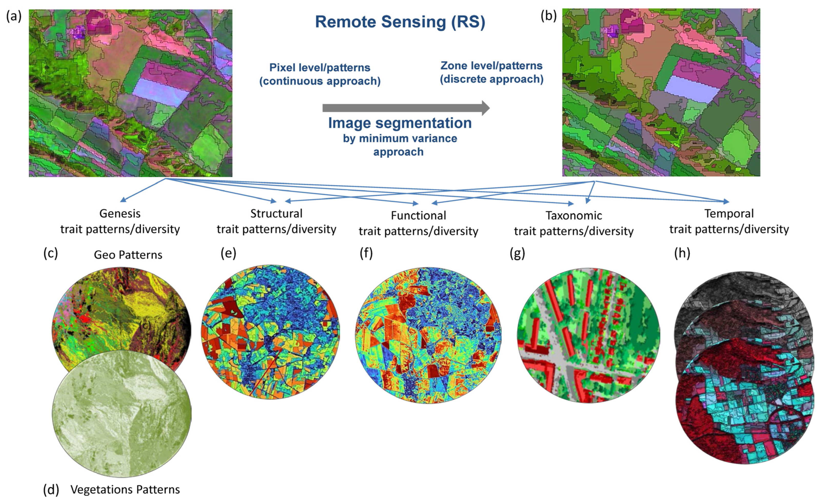
2.4. Creation of Pixels, Zones, Classes and Objects
2.4.1. Pixels
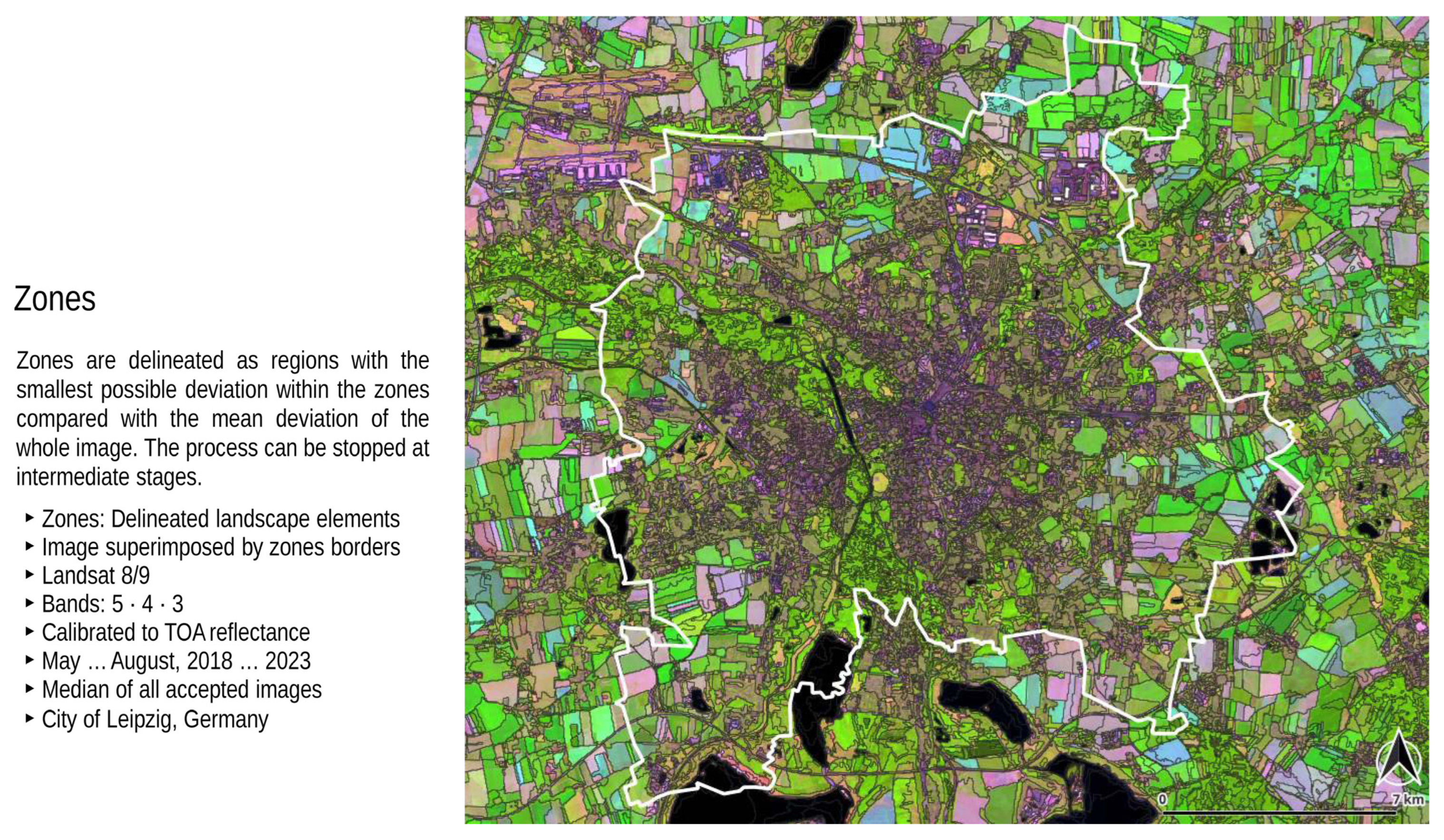
2.4.2. Zones
2.4.3. Classes
2.4.4. Objects
3. Remote Sensing, Data Processing, Analysis and Management in ESIS/Imalys Tool
3.1. Grid-Based Indicators
3.2. Remote Sensing Time Series Indicators
3.3. Kernel Processes for Estimating Raster-Based Indicators
3.4. Indicators by Zone and Raster Indicators by Zone
3.5. Classification Approach
4. Possibilities and Limitations of the ESIS/Imalys Tool
5. Possible Applications of the ESIS/Imalys Tool
- Example 1: Monitoring landscape diversity
- Example 2: Monitoring landscape structure and landscape fragmentation
- Example 3: Monitoring land use intensity and its impact on ecosystem functions
- Monitoring the intensity of urban land use.
- Assessment of the hemeroby or naturalness of landscapes.
- Monitoring vegetation diversity and geodiversity by deriving indicators to quantify genetic diversity, trait diversity, structural diversity, taxonomic diversity and functional diversity.
- Monitoring of species distribution (fauna and flora).
- Monitoring of water quality and its drivers such as LUI.
- Monitoring of vegetation vitality (e.g., bark beetle infections).
- Monitoring of the ecosystem and its processes and changes.
6. Summary and Outlook
Author Contributions
Funding
Data Availability Statement
Acknowledgments
Conflicts of Interest
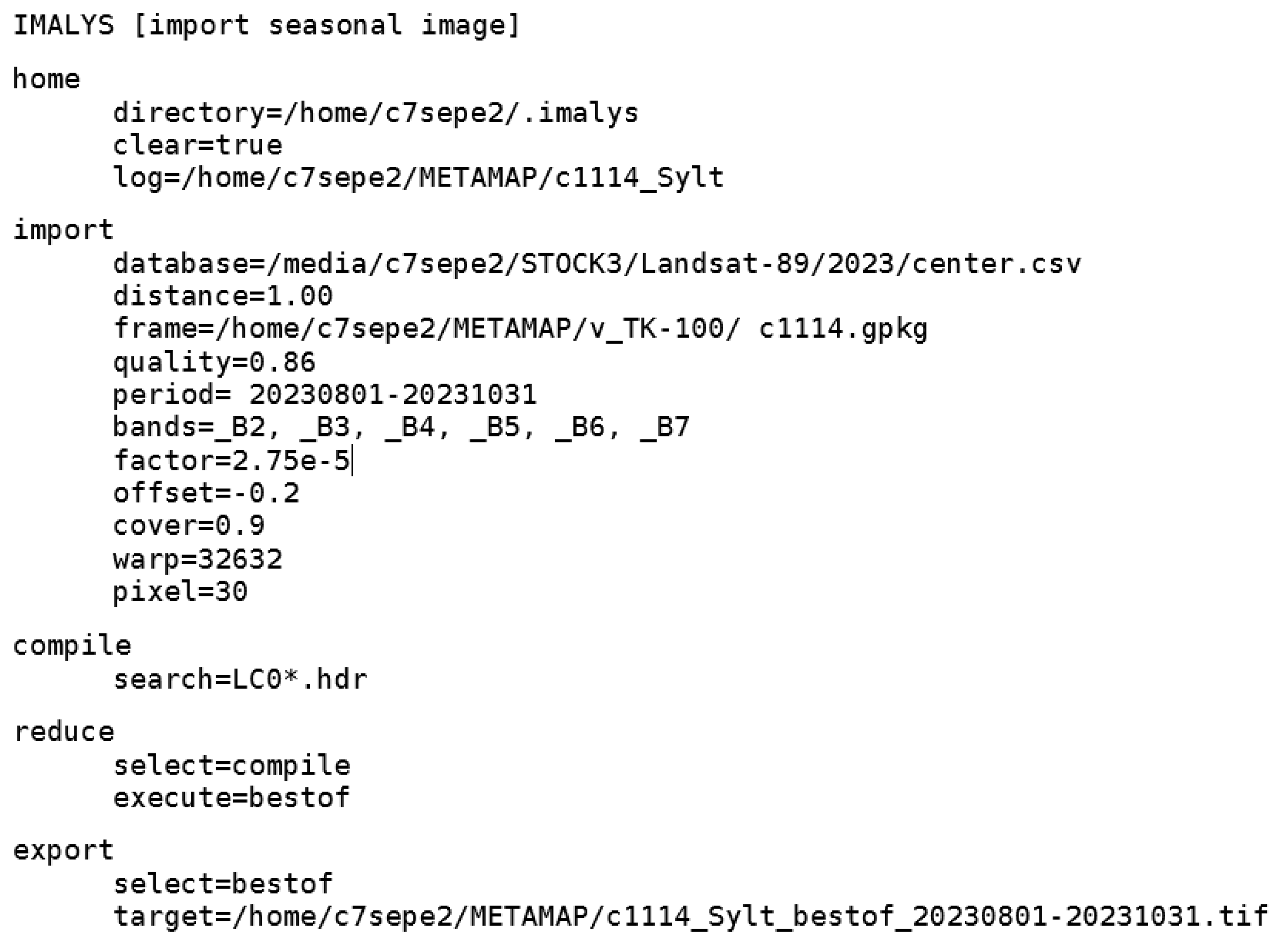
Appendix A. Process Chain Example
Appendix B

| Spectral | ||
| Traits | Description | Formula |
| Variance | Variance based on standard deviation The “variance” command determines the variance of individual pixels based on a standard distribution for all of the bands in source. For multi-image stacks, “Variance” determines the variance for each band separately and gives the result as a multispectral image of the variances. The result can be further reduced to a one band image with the first principal component of all bands using “principal”. | v: values i: items n: item count |
| Regression | Regression based on standard deviation “Regression” returns the regression of individual pixels of all bands in source. “Regression” uses the temporal distance of the recordings from the metadata of the images. To do this, the images must have been imported with “extract” or have been dated afterwards with “extend”. Similar to “variance”, “regression” determines the regression for each band separately if multispectral images are provided and gives a multispectral regression. | t: time v: values i: items n: item count |
| Difference | Euclidean distance of two n-dimensional properties “Difference” gives the difference between the values of two bands or two images. For multispectral images, “difference” generates a result for each band separately and returns a multispectral image of the differences for all bands. | v: pixel value |
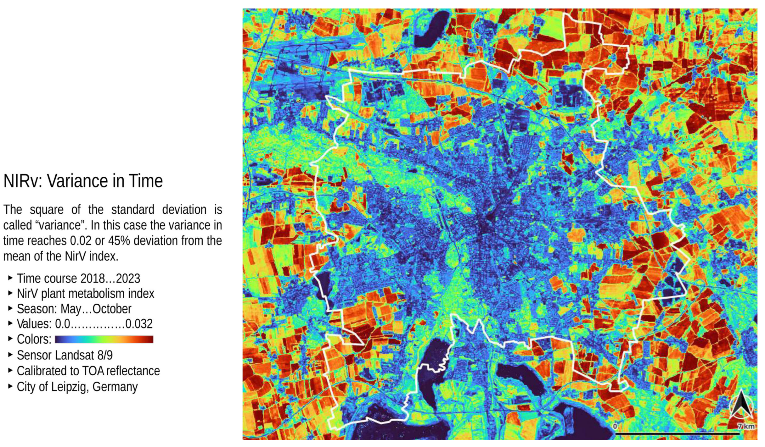
| Vegetation | Near-infrared vegetation index (NIRv) The NIRv index is calculated as the product of near infrared radiation and the normalised difference of the red and the near-infrared radiation. The calculation follows the most common NDVI definition but shows better mapping in sparsely vegetated areas.Vegetation indices were introduced to estimate the plant-covered proportion of the landscape. The result depends on the photosynthetic activity of the plants. Vegetation indices try to quantify the photosynthetically active radiation (PAR) as a measure of plant metabolism. There are about 20 different approximations described [42]. | N: near-infrared value R: red band value Value range: 0…1 |
| Principal | “Principal” gives the first principal component of all bands. The first principal component reflects the brightness or density of all image bands. Imalys uses this process as brightness in several other cases. | v: values i: items |
| Mean | Arithmetic mean, bands or images Mean gives the arithmetic mean of all image bands provided. For multispectral images, “mean” is individually calculated for each band. The process returns a multispectral image of mean values. | v: values i: items n: item count |
| Median | Most common value for each pixel from a stack of bands “Median” reflects the most common value of each pixel in a stack of bands or images. For multiple image stacks, “median” is individually calculated for each band. Median will mask rare values. Image disturbances like clouds or smoke will be masked if more than half of all pixels show an unchanged value. | Value in the middle of a sorted value list. |
| Convolution | ||
| Traits | Description | Formula |
| Texture | ||
| Normal | Normalised texture “Normal” collects the first principal component of all normalised differences between two neighbouring pixels within a given kernel and returns the mean. Landscape diversity increases with texture. The normalised texture is independent of brightness or illumination (shadows). In contrast to Rao’s “entropy” or “roughness”, “normal” will return similar values for regular and randomly distributed patterns. | vi: pixel value vj: neighbour pixel value Value range: 0…1 |
| Inverse | Inverse difference moment (IDM) “Inverse” creates a new image with the inverse difference moment (IDM) proposed by Haralik (Haralik 1979). “Inverse” is particularly high in dark regions and low in bright regions. It can complement “texture” and has proved useful in the analysis of settlement structures. | v: values I,j: neighbor pixels b: bands |
| Roughness (Rao’s Q Index) | Rao‘s diversity based on pixels As “Texture” does, Rao’s approach evaluates the spectral difference of individual pixels, but does not only compare neighbouring pixels, but all pixels within the kernel. Unlike the classical “texture” or “normal” indicators, “roughness” is insensitive for the spatial distribution of the pixels within the kernel. “Roughness” returns a measure for landscape diversity based on pixel differences within a given kernel. Most like “Entropy”, each distribution of a given set of pixels will produce the same result. | dij: Density difference between pixel (i) and (j) pi, pj: Frequency of pixel values (I) and (j) Value range not limited |
| Entropy | Rao‘s entropy (diversity) based on classes “Entropy” collects the number of class differences and class similarities for all pixel combinations within a given kernel. The number of different class combination is scaled with the spectral differences between the classes. Entropy needs a classification of the images to run. The easiest way to obtain this classification is to call the “Mapping” trait. Alternatively, “Entropy” can use an existing classification. “Entropy” returns the diversity of landscape classes within a given kernel. “Entropy” ignores small landscape differences that are represented by the same class and returns a more abstract level. Rao’s approach is insensitive to the distribution of the pixels within the kernel. A chessboard-like distribution of two classes will produce the same result as two homogeneous areas with the same classes. | dkl: spectral Distance between the the classes (k) and (l) pk: frequency of class (k) pl: frequency of class (l)Value range not limited |
| Lowpass | Reduce local contrast “Lowpass” reduces the local contrast of the image data according to the selected “radius”. The process reduces the local contrasts and can fix small bugs. “Lowpass” uses a kernel with a normalised Gaussian distribution. The kernel size can be selected freely. Imalys implements large kernels through an iterative process to significantly reduce the processing time. | v: image values k: kernel values I,j: kernel index |
| Laplace | Enhance local contrast A “Laplace” transformation (Mexican head function) enhances the image contrast and can make lines and closed shapes clearly visible. Imalys implements the transformation as the difference between two Gaussian distributions with a different radius. The parameters “inner” and “outer” control the size (kernel radius) of the two distributions. | v: values k: inner kernel g: outer kernel I,j: kernel indices |
| Create Zones | ||
| Traits | Description | Formula |
| Zones | Delineated homogeneous image elements The “zones” process delineates a seamless network of zones that completely covers the image. The zones are assigned with the spectral signatures of the image data as attributes. The attributes can be expanded (below). “Zones” were introduced to provide a structural basis that can be used for landscape diversity and other structural features. Zones allow for easy transformation of raster images to a vector format like maps. | Structural delineation similar to an inverse watershed. |
| Dendrites | Quotient of zone perimeter and zonal size “Dendrites” returns the quotient between perimeter and size of single zones. Both values grow with larger zones, but the size grows faster. Large zones will show lower values than smaller ones with the same shape. “Dendrites” was introduced as a size-independent measure of spatial diversity. Long and small zones may be quite large but their role in landscape diversity is similar to that of small zones. Small, thin or dendritically shaped zones show high values, large compact zones show the lowest. | vr: result value pz: perimeter (zone) sz: size (zone) Value range: 0…4 |
| Diversity | Spectral diversity for all neighbour zones “Diversity” is calculated as the mean principal component of all spectral differences between all pixels of a single zone. This includes all pixel borders to neighbour zones and also all pixel borders within the zone. The differences are calculated with the zonal mean values, not with individual pixels. “Diversity” was introduced as size-dependent spectral diversity. The principal component intensifies the contrast of single bands. High values indicate small zones and high spectral differences. Small or narrow zones embedded in large zones are emphasized. | vi: zonal value vn: neighbour value bp: pixel borders Value range: 0…1 for reflection values |
| Proportion | Size difference between central zone and all neighbours “Proportion” returns the relation between the size of a single zone and all its neighbours. The result is calculated as difference between the size of the central zone and the mean size of its neighbours. As the size is given on a logarithmic scale, the “mean” is not an arithmetic but a geometric mean. The result will be negative if the central zone is smaller than its neighbours. “Proportion” resembles a texture for zonal sizes. Proportion is independent of the individual size of a zone. Values around zero indicate equally sized neighbour zones. Zones with smaller neighbours show positive values; zones with larger neighbours are negative. | si: size, central zone sj: size, neighbour zone n: number of neighbours |
| Relation | Quotient of cell perimeter and number of neighbours “Relation” is calculated as the relation between the perimeter of the zone and the number of neighbouring zones. “Relation” was introduced as an indicator for spatial diversity. Large zones and small zones with few neighbours will have large values. Small zones with many neighbours will show higher values. Like “Dendrites”, “relation” also returns information about the shape and the connection of the zones. Zones with many connections may provide paths for animal travels and enhance diversity. | R: relation p: perimeter c: number of neighbours |
| Size | Size of one zone given as natural logarithm The zonal size is calculated from the sum of pixels covering the zone. Landscape diversity increases with smaller zones | a: area of zone [ha] |
| Diffusion | Smooth properties in a zones network The algorithm for value equalisation in zones mimics diffusion through membranes (borders). In the process, features “migrate” into the neighbouring zone like soluble substances and combine with existing concentrations. The intensity of diffusion depends on the length of the common border and the number of iterations. The size of the zones does not matter. The process is only controlled by the number of iterations. Each iteration includes a new layer of contributing zones. The influence of distant zones on the central zone decreases with distance. Entries over 10 are still allowed, but rarely have a visible effect. | a: attribute s: zone size b: border length i,j: zone indices t: iterations (time) |
| External | ||
| Values | Raster representation of a vector map with attributes “Values” creates a multiband raster image from vector borders and the attributes of the different polygons. “Values” mainly serves as a control feature. | Raster image from vector polygons |
| Classification | ||
| Trait/Tool | Description | Process |
| Pixel | “Pixel” classifies spectral combinations “Pixel” selects a pixel-oriented classification of the image data. The process uses all bands of the provided image. The process is controlled only by the number of classes in the result. All values should have a comparable value range, as calibrated images do. | Fully self-adjusting classification of all pixel values |
| Features | “Features” classifies spectral and spatial properties of zones “Features” selects the classification of zones based on their features. The process is controlled by the selected features and by the number of classes in the result. Each feature can be selected individually. As with “pixels”, the value range of the features should be comparable. | Fully self-adjusting classification of all zones’ features |
| Fabric (Objects) | “Fabric” creates and classifies image objects In this context, adjacent zones with an individual combination of different features are called objects. Object types (classes) and image objects are created during the same process. The object definition relays only on the borders between different types of zones. Thus, objects are characterized by their spatial pattern. | Fully self-adjusting delineation and classification of image objects based on zones with different features. |
| Compare | Compare a mapping with a reference Automated classification is driven by image features. Real classes are not necessarily defined by their appearance. “compare” allows for evaluating if and up to what degree real classes can be detected by image features. | Confusion matrix for false and true detection and denotation |
| Rank | Correlate distributions “Rank” calculates a correlation coefficient based on a rank correlation model after Spearman. A rank correlation is independent of the basic value distribution. Therefore, it can be used for each set of data. | r,s: item rank i: item index n: item count |
| Export | ||
| Traits | Description | Process |
| Raster | Export values using an image raster format Images and processing results can be exported in 48 different raster formats (according to most recent gdal library). Raster export includes vector-based process results. Standard format is ENVI labelled. | gdal library |
| Vector | Export values using a vector format Vector-based results can be exported using 23 different vector formats (according to most recent gdal library). Vector export includes automated transformation for most of the raster data. Standard formats are ESRI Shape and CSV. | gdal library |
| Table | Export tables using a table format Value grids can be exported in different database and spreadsheet formats. Table export includes tables linked to raster or vector data. The standard format is CSV. | gdal library |
References
- Intergovernmental Panel on Climate Change. Climate Change and Land; Cambridge University Press: Cambridge, UK, 2022; ISBN 9781009157988. [Google Scholar]
- Skidmore, A.K.; Coops, N.C.; Neinavaz, E.; Ali, A.; Schaepman, M.E.; Paganini, M.; Kissling, W.D.; Vihervaara, P.; Darvishzadeh, R.; Feilhauer, H.; et al. Priority list of biodiversity metrics to observe from space. Nat. Ecol. Evol. 2021, 5, 896–906. [Google Scholar] [CrossRef] [PubMed]
- Lausch, A.; Selsam, P.; Pause, M.; Bumberger, J. Monitoring vegetation- and geodiversity with remote sensing and traits. Philos. Trans. R. Soc. A Math. Phys. Eng. Sci. 2024, 382, 20230058. [Google Scholar] [CrossRef] [PubMed]
- Lausch, A.; Schaepman, M.E.; Skidmore, A.K.; Catana, E.; Bannehr, L.; Bastian, O.; Borg, E.; Bumberger, J.; Dietrich, P.; Glässer, C.; et al. Remote Sensing of Geomorphodiversity Linked to Biodiversity—Part III: Traits, Processes and Remote Sensing Characteristics. Remote Sens. 2022, 14, 2279. [Google Scholar] [CrossRef]
- Schrodt, F.; Vernham, G.; Bailey, J.; Field, R.; Gordon, J.E.; Gray, M.; Hjort, J.; Hoorn, C.; Hunter, M.L., Jr.; Larwood, J.; et al. The status and future of essential geodiversity variables. Philos. Trans. R. Soc. A Math. Phys. Eng. Sci. 2024, 382, 20230052. [Google Scholar] [CrossRef] [PubMed]
- Kuemmerle, T.; Erb, K.; Meyfroidt, P.; Müller, D.; Verburg, P.H.; Estel, S.; Haberl, H.; Hostert, P.; Jepsen, M.R.; Kastner, T.; et al. Challenges and opportunities in mapping land use intensity globally. Curr. Opin. Environ. Sustain. 2013, 5, 484–493. [Google Scholar] [CrossRef] [PubMed]
- Burkhard, B.; Kroll, F.; Nedkov, S.; Müller, F. Mapping ecosystem service supply, demand and budgets. Ecol. Indic. 2012, 21, 17–29. [Google Scholar] [CrossRef]
- Haase, P.; Tonkin, J.D.; Stoll, S.; Burkhard, B.; Frenzel, M.; Geijzendorffer, I.R.; Häuser, C.; Klotz, S.; Kühn, I.; McDowell, W.H.; et al. The next generation of site-based long-term ecological monitoring: Linking essential biodiversity variables and ecosystem integrity. Sci. Total Environ. 2018, 613–614, 1376–1384. [Google Scholar] [CrossRef]
- Mollenhauer, H.; Kasner, M.; Haase, P.; Peterseil, J.; Wohner, C.; Frenzel, M.; Mirtl, M.; Schima, R.; Bumberger, J.; Zacharias, S. Science of the Total Environment Long-term environmental monitoring infrastructures in Europe: Observations, measurements, scales, and socio-ecological representativeness Group on Earth Observations Global Earth Observation System of Systems. Sci. Total Environ. 2018, 624, 968–978. [Google Scholar] [CrossRef]
- Weber, U.; Attinger, S.; Baschek, B.; Boike, J.; Borchardt, D.; Brix, H.; Brüggemann, N.; Bussmann, I.; Dietrich, P.; Fischer, P.; et al. MOSES: A Novel Observation System to Monitor Dynamic Events across Earth Compartments. Bull. Am. Meteorol. Soc. 2022, 103, E339–E348. [Google Scholar] [CrossRef]
- Zhao, Z.; Martin, P.; Grosso, P.; Los, W.; de Laat, C.; Jeffrey, K.; Hardisty, A.; Vermeulen, A.; Castelli, D.; Legre, Y.; et al. Reference Model Guided System Design and Implementation for Interoperable Environmental Research Infrastructures. In Proceedings of the 2015 IEEE 11th International Conference on e-Science, Munich, Germany, 31 August–4 September 2015; pp. 551–556. [Google Scholar]
- Likens, G.E. Aldo Leopold’s “Odyssey” and the development of the ecosystem concept and approach. Socio-Ecol. Pract. Res. 2022, 4, 17–18. [Google Scholar] [CrossRef]
- Rocchini, D.; Santos, M.J.; Ustin, S.L.; Féret, J.; Asner, G.P.; Beierkuhnlein, C.; Dalponte, M.; Feilhauer, H.; Foody, G.M.; Geller, G.N.; et al. The Spectral Species Concept in Living Color. J. Geophys. Res. Biogeosci. 2022, 127, e2022JG007026. [Google Scholar] [CrossRef]
- Cavender-Bares, J.; Gamon, J.A.; Townsend, P.A. Remote Sensing of Plant Biodiversity; Cavender-Bares, J., Gamon, J.A., Townsend, P.A., Eds.; Springer International Publishing: Cham, Switzerland, 2020; ISBN 978-3-030-33156-6. [Google Scholar]
- Zarnetske, P.; Read, Q.; Record, S.; Gaddis, K.; Pau, S.; Hobi, M.; Malone, S.; Costanza, J.; Dahlin, K.; Latimer, A.; et al. Towards connecting biodiversity and geodiversity across scales with satellite remote sensing. Glob. Ecol. Biogeogr. 2019, 28, 548–556. [Google Scholar] [CrossRef]
- Lausch, A.; Schaepman, M.E.; Skidmore, A.K.; Truckenbrodt, S.C.; Hacker, J.M.; Baade, J.; Bannehr, L.; Borg, E.; Bumberger, J.; Dietrich, P.; et al. Linking the Remote Sensing of Geodiversity and Traits Relevant to Biodiversity—Part II: Geomorphology, Terrain and Surfaces. Remote Sens. 2020, 12, 3690. [Google Scholar] [CrossRef]
- Kussul, N.; Lavreniuk, M.; Skakun, S.; Shelestov, A. Deep Learning Classification of Land Cover and Crop Types Using Remote Sensing Data. IEEE Geosci. Remote Sens. Lett. 2017, 14, 778–782. [Google Scholar] [CrossRef]
- Wellmann, T.; Haase, D.; Knapp, S.; Salbach, C.; Selsam, P.; Lausch, A. Urban land use intensity assessment: The potential of spatio-temporal spectral traits with remote sensing. Ecol. Indic. 2018, 85, 190–203. [Google Scholar] [CrossRef]
- Xie, C.; Wang, J.; Haase, D.; Wellmann, T.; Lausch, A. Measuring spatio-temporal heterogeneity and interior characteristics of green spaces in urban neighborhoods: A new approach using gray level co-occurrence matrix. Sci. Total Environ. 2023, 855, 158608. [Google Scholar] [CrossRef]
- Chabrillat, S.; Segl, K.; Foerster, S.; Brell, M.; Guanter, L.; Schickling, A.; Storch, T.; Honold, H.-P.; Fischer, S. EnMAP Pre-Launch and Start Phase: Mission Update. In Proceedings of the IGARSS 2022–2022 IEEE International Geoscience and Remote Sensing Symposium, Kuala Lumpur, Malaysia, 17–22 July 2022; pp. 5000–5003. [Google Scholar]
- Cerra, D.; Marshall, D.; Heiden, U.; Alonso, K.; Bachmann, M.; Burch, K.; Carmona, E.; Dietrich, D.; Lester, H.; Knodt, U.; et al. The Spaceborne Imaging Spectrometer Desis: Data Access, Outreach Activities, and Scientific Applications. In Proceedings of the IGARSS 2022–2022 IEEE International Geoscience and Remote Sensing Symposium, Kuala Lumpur, Malaysia, 17–22 July 2022; pp. 5395–5398. [Google Scholar]
- Coyle, D.B.; Stysley, P.R.; Chirag, F.L.; Frese, E.A.; Poulios, D. The Global Ecosystem Dynamics Investigation (GEDI) LiDAR laser transmitter. In Infrared Remote Sensing and Instrumentation XXVII: 12–14 August 2019, San Diego, California, United States; Strojnik, M., Arnold, G.E., Eds.; SPIE: Bellingham, WA, USA, 2019; p. 20. [Google Scholar]
- Cawse-Nicholson, K.; Townsend, P.A.; Schimel, D.; Assiri, A.M.; Blake, P.L.; Buongiorno, M.F.; Campbell, P.; Carmon, N.; Casey, K.A.; Correa-Pabón, R.E.; et al. NASA’s surface biology and geology designated observable: A perspective on surface imaging algorithms. Remote Sens. Environ. 2021, 257, 112349. [Google Scholar] [CrossRef]
- Le Provost, G.; Thiele, J.; Westphal, C.; Penone, C.; Allan, E.; Neyret, M.; van der Plas, F.; Ayasse, M.; Bardgett, R.D.; Birkhofer, K.; et al. Contrasting responses of above- and belowground diversity to multiple components of land-use intensity. Nat. Commun. 2021, 12, 3918. [Google Scholar] [CrossRef]
- Palmer, M.W.; Earls, P.G.; Hoagland, B.W.; White, P.S.; Wohlgemuth, T. Quantitative tools for perfecting species lists. Environmetrics 2002, 13, 121–137. [Google Scholar] [CrossRef]
- Rocchini, D.; Chiarucci, A.; Loiselle, S.A. Testing the spectral variation hypothesis by using satellite multispectral images. Acta Oecol. 2004, 26, 117–120. [Google Scholar] [CrossRef]
- Conti, L.; Malavasi, M.; Galland, T.; Komárek, J.; Lagner, O.; Carmona, C.P.; Bello, F.; Rocchini, D.; Šímová, P. The relationship between species and spectral diversity in grassland communities is mediated by their vertical complexity. Appl. Veg. Sci. 2021, 24, e12600. [Google Scholar] [CrossRef]
- Ustin, S.L.; Gamon, J.A. Remote sensing of plant functional types. New Phytol. 2010, 186, 795–816. [Google Scholar] [CrossRef]
- Díaz, S.; Kattge, J.; Cornelissen, J.H.C.; Wright, I.J.; Lavorel, S.; Dray, S.; Reu, B.; Kleyer, M.; Wirth, C.; Colin Prentice, I.; et al. The global spectrum of plant form and function. Nature 2016, 529, 167–171. [Google Scholar] [CrossRef]
- Lausch, A.; Erasmi, S.; King, D.; Magdon, P.; Heurich, M. Understanding Forest Health with Remote Sensing-Part I—A Review of Spectral Traits, Processes and Remote-Sensing Characteristics. Remote Sens. 2016, 8, 1029. [Google Scholar] [CrossRef]
- Andersson, E.; Haase, D.; Anderson, P.; Cortinovis, C.; Goodness, J.; Kendal, D.; Lausch, A.; McPhearson, T.; Sikorska, D.; Wellmann, T. What are the traits of a social-ecological system: Towards a framework in support of urban sustainability. NPJ Urban Sustain. 2021, 1, 14. [Google Scholar] [CrossRef]
- Lausch, A.; Blaschke, T.; Haase, D.; Herzog, F.; Syrbe, R.-U.; Tischendorf, L.; Walz, U. Understanding and quantifying landscape structure—A review on relevant process characteristics, data models and landscape metrics. Ecol. Modell. 2015, 295, 31–41. [Google Scholar] [CrossRef]
- McGarigal, K.; Marks, B.J. FRAGSTATS: Spatial Pattern Analysis Program for Quantifying Landscape Structure; U.S. Department of Agriculture, Forest Service, Pacific Northwest Research Station: Portland, OR, USA, 1995. [Google Scholar]
- McGarigal, K.; Cushman, S.A. The gradient concept of landscape structure. In Issues and Perspectives in Landscape Ecology; Cambridge University Press: Cambridge, UK, 2005; pp. 112–119. [Google Scholar]
- Blaschke, T. Object based image analysis for remote sensing. ISPRS J. Photogramm. Remote Sens. 2010, 65, 2–16. [Google Scholar] [CrossRef]
- Blaschke, T.; Hay, G.J.; Kelly, M.; Lang, S.; Hofmann, P.; Addink, E.; Queiroz Feitosa, R.; van der Meer, F.; van der Werff, H.; van Coillie, F.; et al. Geographic Object-Based Image Analysis—Towards a new paradigm. ISPRS J. Photogramm. Remote Sens. 2014, 87, 180–191. [Google Scholar] [CrossRef] [PubMed]
- Kralisch, S.; Böhm, B.; Böhm, C.; Busch, C.; Fink, M.; Fischer, C.; Schwartze, C.; Selsam, P.; Zander, F.; Flügel, W.A. ILMS—A Software Platform for Integrated Environmental Management. International Congress on Environmental Modelling and Software. 206. Available online: https://scholarsarchive.byu.edu/iemssconference/2012/Stream-B/206 (accessed on 19 March 2024).
- Zander, F.; Kralisch, S.; Busch, C.; Flügel, W.-A. Data management in multidisciplinary research projects with the River Basin information System. EnviroInfo 2012, 143–149. [Google Scholar]
- Selsam, P.; Schwartze, C. Remote Sensing Image Analysis Without Expert Knowledge—A Web-Based Classification Tool On Top of Taverna Workflow Management System. IOP Conf. Ser. Earth Environ. Sci. 2016, 44, 042020. [Google Scholar] [CrossRef]
- Selsam, P.; Gey, R.; Lausch, A.; Bumberger, J. Imalys—Image Analysis (0.1). Zenodo 2023. [Google Scholar] [CrossRef]
- Rocchini, D.; Bacaro, G.; Chirici, G.; Da Re, D.; Feilhauer, H.; Foody, G.M.; Galluzzi, M.; Garzon-Lopez, C.X.; Gillespie, T.W.; He, K.S.; et al. Remotely sensed spatial heterogeneity as an exploratory tool for taxonomic and functional diversity study. Ecol. Indic. 2018, 85, 983–990. [Google Scholar] [CrossRef]
- Badgley, G.; Field, C.B.; Berry, J.A. Canopy near-infrared reflectance and terrestrial photosynthesis. Sci. Adv. 2017, 3, e1602244. [Google Scholar] [CrossRef]
- Rocchini, D.; Marcantonio, M.; Ricotta, C. Measuring Rao’s Q diversity index from remote sensing: An open source solution. Ecol. Indic. 2017, 72, 234–238. [Google Scholar] [CrossRef]
- Rocchini, D.; Luque, S.; Pettorelli, N.; Bastin, L.; Doktor, D.; Faedi, N.; Feilhauer, H.; Féret, J.; Foody, G.M.; Gavish, Y.; et al. Measuring β-diversity by remote sensing: A challenge for biodiversity monitoring. Methods Ecol. Evol. 2018, 9, 1787–1798. [Google Scholar] [CrossRef]
- Xu, Q.; Wang, P.; Shu, W.; Ding, M.; Zhang, H. Influence of landscape structures on river water quality at multiple spatial scales: A case study of the Yuan river watershed, China. Ecol. Indic. 2021, 121, 107226. [Google Scholar] [CrossRef]
- Pu, X.; Cheng, Q. Unraveling the impacts of multiscale landscape patterns and socioeconomic development on water quality: A case study of the National Sustainable Development Agenda Innovation Demonstration Zone in Lincang City, Southwest China. J. Hydrol. Reg. Stud. 2024, 51, 101660. [Google Scholar] [CrossRef]
- Xiao, H.; Su, R.; Luo, Y.; Jiang, Y.; Wang, Y.; Hu, R.; Lin, S. Effects of land cover patterns on pond water nitrogen and phosphorus concentrations in a small agricultural watershed in Central China. Catena 2024, 237, 107800. [Google Scholar] [CrossRef]


Disclaimer/Publisher’s Note: The statements, opinions and data contained in all publications are solely those of the individual author(s) and contributor(s) and not of MDPI and/or the editor(s). MDPI and/or the editor(s) disclaim responsibility for any injury to people or property resulting from any ideas, methods, instructions or products referred to in the content. |
© 2024 by the authors. Licensee MDPI, Basel, Switzerland. This article is an open access article distributed under the terms and conditions of the Creative Commons Attribution (CC BY) license (https://creativecommons.org/licenses/by/4.0/).
Share and Cite
Selsam, P.; Bumberger, J.; Wellmann, T.; Pause, M.; Gey, R.; Borg, E.; Lausch, A. Ecosystem Integrity Remote Sensing—Modelling and Service Tool—ESIS/Imalys. Remote Sens. 2024, 16, 1139. https://doi.org/10.3390/rs16071139
Selsam P, Bumberger J, Wellmann T, Pause M, Gey R, Borg E, Lausch A. Ecosystem Integrity Remote Sensing—Modelling and Service Tool—ESIS/Imalys. Remote Sensing. 2024; 16(7):1139. https://doi.org/10.3390/rs16071139
Chicago/Turabian StyleSelsam, Peter, Jan Bumberger, Thilo Wellmann, Marion Pause, Ronny Gey, Erik Borg, and Angela Lausch. 2024. "Ecosystem Integrity Remote Sensing—Modelling and Service Tool—ESIS/Imalys" Remote Sensing 16, no. 7: 1139. https://doi.org/10.3390/rs16071139
APA StyleSelsam, P., Bumberger, J., Wellmann, T., Pause, M., Gey, R., Borg, E., & Lausch, A. (2024). Ecosystem Integrity Remote Sensing—Modelling and Service Tool—ESIS/Imalys. Remote Sensing, 16(7), 1139. https://doi.org/10.3390/rs16071139