A Lightning Optical Automatic Detection Method Based on a Deep Neural Network

Abstract

To achieve automatic recognition of lightning images, which cannot easily be handled using the existing methods and still requires significant human resources, we propose a lightning image dataset and a preprocessing method. The lightning image data over five months were collected using a camera based on two optical observation stations, and then a series of batch labeling methods were applied, which greatly reduced the workload of subsequent manual labeling, and a dataset containing more than 30,000 labeled samples was established. Considering that lightning varies rapidly over time, we propose a time sequence composite (TSC) preprocessing method that inputs lightning’s time-varying characteristics into a model for better recognition of lightning images. The TSC method was evaluated through an experiment on four backbones, and it was found that this preprocessing method enhances the classification performance by 40%. The final trained model could successfully distinguish between the “lightning” and “non-lightning” samples, and a recall rate of 86.5% and a false detection rate of 0.2% were achieved.

1. Introduction

Lightning is a natural strong discharge phenomenon that emits electromagnetic, optical, and acoustic signals when it occurs. By monitoring and analyzing the signal data, we can study the characteristics of lightning [1,2,3,4,5,6,7,8,9,10]. Among these signals, the optical data are important because they not only reveal the actual morphology of the lightning but also serve as the truth value to verify the detection efficiency and location accuracy of the lightning location system [11], which has broad application prospects. In the 1930s, the research team of Schonland and Malan [12] observed lightning with the invention of a mechanical streak camera and revealed the process of lightning discharge, which greatly contributed to the development of lightning research. In 1990, Yokoyama [13] designed a lightning observation system based on a high-speed camera, and since then, more detailed results have been obtained using high-speed cameras in lightning observation. Jiang and Qie et al. [14] observed the complete two-way propagation of lightning based on a high-speed camera and recorded many of lightning’s physical processes [15,16,17,18,19]. Kong et al. [20] used a high-speed camera to observe the stepped extension of positive-polarity lightning. Lu et al. [21,22,23,24,25,26,27,28] set up the Lightning Observation System for Tall Buildings in Guangzhou (TOLOG) and made many observations of lightning in Guangdong. For example, a complete record of six-branched lightning was analyzed, and it was also found that one upward streak of lightning could trigger another upward streak of lightning of the opposite polarity from a nearby tall and grounded object. Wang et al. [29,30] recorded five types of triggered lightning bolts using a high-speed camera and fast antenna instruments and analyzed the phenomenon of lightning with multiple branches. In addition, transient luminous events over thunderstorms have been observed using a high-sensitivity camera (e.g., Winckler et al., 1989, Pasko et al., 2002, Van der Velde et al., 2009, Yang et al., 2017) [31,32,33,34]. Yang et al. [34] analyzed a single sprite produced using a mesoscale convective system (MCS). In addition, the spectra of the lightning were observed [35,36], and its physical parameters, such as the electron temperature, density, and conductivity in the channel, were quantitatively calculated, thus allowing the microphysical information inside and around the channel to be obtained.

It is worth noting that the optical observations of lightning described above are generally recorded through manual triggering, which requires considerable human resources to achieve without any intelligent method to acquire the lightning image data automatically. However, automatic recognition of lightning images is very complicated: (1) lightning does not have a fixed shape like normal objects but is an intensely luminous ionized channel, and the position of the lightning’s appearance and its channel shape are highly random; (2) optical observations may be affected by weather, such as strong winds and heavy rain, which may lead to shaky and distorted images; (3) the optical signal can be easily scattered, resulting in the lightning being partially or completely obscured by clouds or rain curtains; (4) moving objects (e.g., birds, bugs, and human activities) bring more variability and complicate the problem. All these factors make the classification of “lightning” and “non-lightning” very difficult. For such a complex classification task, a deep neural network (DNN) is a good choice.

DNNs have made great progress in recent years, and the following research advances are related to computer vision backbones for object recognition. LeNet-5, proposed by Yann LeCun [37], was widely used in handwritten image recognition in 1998. Alex Krizhevsky et al. [38] trained a model called AlexNet, which was one of the largest convolutional neural networks (CNNs) to date, on subsets of ImageNet with a top five error rate of 17%. In 2014, Christain et al. [39] developed GoogleNet, which used fewer parameters than AlexNet but improved the utilization of computing resources within the network and won the ILSVRC with an error rate of less than 7%. ResNet, proposed by He et al. in 2016 [40], introduced shortcuts that solved the problem of model degradation after deepening the model layers. Zagoruyko et al. [41] tried to use a shallower but wider model to improve the performance of the model and finally proposed Wide-ResNet, which is faster to train than ResNet. In ResNeXt, proposed by Xie et al. [42], the concept of cardinality is introduced. The accuracy of the network can be continuously improved by increasing the number of branches in the block, and the diminishing returns can be increased from the width and depth of the model, which also simplifies the network design. Huang et al. [43] proposed DenseNet in 2017, whose core structure, DenseBlock, differs from ResBlock in the reuse of feature maps, and they strengthened the feature propagation, encouraged feature reuse, and substantially reduced the number of parameters. The development of deep neural networks has also brought about new tools for weather-related image recognition tasks. For example, Zhao et al. [44] realized multi-label weather recognition in static images using CNN-RNN, and Lv et al. [45] proposed a cloud map classification method based on comparative self-supervised learning.

In this paper, lightning image recognition based on a DNN is implemented, but a large, labeled dataset is required to train the model, and there is no existing dataset that can be used for the lightning image recognition task. Therefore, we constructed the first lightning image dataset and designed experiments to achieve automatic recognition of lightning images. The main contributions of this paper lie in the following two aspects: (1) a series of batch labeling methods are proposed in the establishment of the dataset, which greatly reduces the workload of manually labeling the dataset; (2) the dataset is preprocessed according to the characteristics of the lightning image recognition task so that the time-varying features of lightning can be put into the model. Meanwhile, the model already has a strong capability for spatial feature extraction. Combining the dataset and the methodology of this paper, a benchmark for lightning image recognition is proposed, and end-to-end lightning image recognition has been realized.

This paper is organized as follows: Section 1 is the introduction; Section 2 introduces the data sources for this paper; Section 3 describes the two methods proposed in this paper to solve the problem; Section 4 describes the classification of the dataset and analyzes the dataset to provide a more comprehensive perspective; Section 5 describes lightning image classification experiments conducted based on the dataset to validate the effectiveness of the preprocessing methods proposed in this paper; Section 6 concludes with a summary and outlook.

2. Data and Methods

2.1. Data Source

Two optical observation stations were built by the research team of Nanjing University of Information Science and Technology (NUIST) in 2022, located in Xuwen (located at 20.3°N, 110.1°E), Hainan Province, and Nanjing (located at 32.1°N, 118.7°E), Jiangsu Province. The time periods for data collection were from April to August in 2022 and from June to July in 2023. Two fixed-direction cameras were installed at the Xuwen station, and two fixed-directional cameras and an all-sky camera were installed at the Nanjing station. The fixed-direction cameras have a field of horizontal view of 60° and a field of vertical view of 40°, and each camera shoots in a different direction. The horizontal field of view of the all-sky camera is 360°, and the vertical field of view is 90°, which distorts the image. However, lightning is a luminous belt without a fixed shape, so the distortion cannot affect the recognition. How far the lightning can be observed is mainly determined by the air visibility along the transmission path and the intensity of the lightning. By observing the existing data, we determined that this distance could not exceed 10 km. The azimuth direction relative to the true north of the two cameras in Nanjing is 150° and 210°, respectively. The azimuth direction relative to the true north of the two cameras in Xuwen is 120° and 180°, respectively.

The video files captured using the two cameras have a resolution of 1280 × 1024, a frame rate of 60 fps, an AVI video format, and a length of 30 s. Although 60 fps is referred to as the normal speed and researchers prefer to use high-speed video to conduct research on lightning, we first developed automatic lightning image recognition using a video at normal speed. The methodology in this paper is compatible with high-speed video, and only some details need to be adjusted (e.g., the frames can be merged to have a lower fps).

By continuously acquiring data, the five cameras can produce a total of 14,400 video files per day. The displayed samples in Figure 1 are taken from a single frame of the lightning’s occurrence, which usually has one of the following characteristics: (1) a clear luminous channel or (2) a sudden bright spot in the cloud.

2.2. Batch Labeling Method

Two optical observation stations produce 14,400 video files per day, each with 1800 frames; therefore, it is impossible to manually label each frame to indicate whether it is lightning or not. Therefore, a series of batch labeling methods were proposed, which can batch-label most of the non-lightning samples. The remaining samples that had a high possibility of containing lightning were manually labeled. Quality control was performed for all the samples during the final manual labeling by visually checking the existence of lightning. The processing flow is shown in Figure 2. This is mainly based on the following considerations: (1) due to the rare occurrence of lightning, most samples are non-lightning samples; (2) most non-lightning samples have significant and easily extractable features; (3) non-lightning segments tend to be static or quasi-static, which can be clipped to reduce the total number of samples and avoid extra model training time costs.

2.2.1. Pre-Screening Methods

The pre-screening method compares every two successive frames in the video file, removes the video file without content variation, and merges the segments with little difference. The value of the difference between the frames is obtained by summing the absolute values of the subtraction between the two. If the value of difference is greater than an experimentally determined threshold, it is defined that there is difference between the two frames. For a video file, the first frame is marked as the HEAD frame, and it is compared with the next frame; if there is a difference, the next frame is marked as the new HEAD frame and continues to be compared with the others. If there is no difference, then the HEAD frame continues to be compared with the rest. In the end, a video file with only one HEAD frame is deleted because the only HEAD frame is not different from the rest of the frames; if there are frames with a difference, which means more than one HEAD frame exist, then the video file is kept, and the HEAD frame information is saved. Video files that are almost completely black at night can be removed through pre-screening, and video files that contain minor differences during the day, such as sunny and cloudy days, can be clipped into slices including HEAD frames and their “tail” frames. In the next step of batch labeling, the “tail” frames were ignored, effectively reducing the total number of samples.

2.2.2. Rough Batch Labeling

The significant time-varying characteristics of the video files containing lightning were observed during analysis of the collected data, and most video files without lightning were static or quasi-static. Therefore, feature quantity 1 (FQ1) was proposed to quickly screen videos without lightning by analyzing the rate of change in the video. It is calculated as follows. For a video file, the absolute values of each pixel difference between two frames are first calculated, and then the variance is solved for all the values, so that one value can be obtained for every two successive frames. On the basis of this value, the variance is solved for all the values calculated for every two successive frames. Finally, FQ1 is obtained. FQ1 calculates the variance in the overall picture (i.e., spatial) and involves the variance in the temporal sequence. Based on FQ1 and an experimentally derived threshold (the thresholds of FQ1 and FQ2 were obtained using a loop of adjusting the threshold and observing the results of batch labeling), all the static and quasi-static video files were filtered, i.e., all the samples generated from the filtered video file were uniformly labeled as non-lightning.

Anomalous perturbations caused by windy weather can produce too large a value for FQ1, resulting in a considerable number of non-lightning video files still failing to be labeled. Therefore, the following method is used to calculate feature quantity 2 (FQ2), which can label non-lightning video files in the range that FQ1 fails to label and alleviate the influence of abnormal perturbations. The method of calculation is as follows. (1) A subsequence of five frames is clipped from the video and scanned in a small grid of 256 × 256 × 5 with the half-side as the step size. (2) The content within the entire grid (5 frames) is normalized once, and then the average value of each frame is sought separately. (3) If the average value of these 5 frames conforms to a rising and then falling trend, then the maximum value minus the minimum value is the FQ2 of the current grid; otherwise, it is set to 0. (4) This calculation is performed for the entire video file in steps of 1 frame, and the maximum value of the FQ2 of all the grids is finally used as the FQ2 of the entire video file. FQ2 calculates the fluctuation in the local luminance for a short period of time, and only the fluctuation in the luminance in the 5 frames forms a rising and then falling trend. Based on FQ2 and an experimentally derived threshold, the video files with shaking but without lightning were filtered and labeled as non-lightning. However, for videos with violent shaking, FQ2 was still unable to distinguish them well.

2.2.3. Fine Batch Labeling

After most of the non-lightning videos were labeled using FQ1 and FQ2, there were still many static and quasi-static segments in the rest of the video files that could not be batch-labeled. Therefore, a light pulse extraction method was proposed using the following idea: most lightning is presented as a light pulse in the video, i.e., the overall brightness of the frame rises violently before falling, and the light pulse corresponding to lightning can be distinguished. To extract the light pulses, the average brightness of each frame is first calculated. If the difference between this average and the before and after is positive and greater than an experimentally derived threshold, the corresponding frame is a light pulse and potentially lightning, which requires further manual labeling. The rest of the frames are labeled as non-lightning based on the information recorded during pre-screening, i.e., only HEAD frames are labeled as non-lightning.

2.3. Time Sequence Composite (TSC) Preprocessing Methods

Although existing models can extract the spatial features of the samples, the lightning image recognition task is unique compared to a general image recognition task. First, the spatial features of the samples have a considerable probability of being influenced by weather, animal activity, etc., as mentioned in the introduction, and the morphology of lightning is unstable compared to general objects (e.g., ships, cars, etc.) because lightning is a luminous ionized channel. Second, due to the significant time-varying characteristics of lightning, it is better to put such characteristics into the model instead of a static lightning picture. Therefore, we proposed the TSC preprocessing method, as shown in Figure 3: a series of 3 frames that are centered by the labeled frame are composed into a 3 × W × H picture, where each frame corresponds to one of the RGB channels. Using such a preprocessing method, the following two points are considered:

For most lightning, 3 frames are long enough to encompass it, and the optical acquisition device used in this paper has a recording frame rate of 60 fps. For a very small portion of continuous lightning, the light pulse extraction method can break it down into multiple pulses, which can deal with lightning of any length.

Increasing the number of channels (e.g., performing the TSC method for 5 frames, using 5 × W × H inputs) will result in a greater consumption of memory and computing power.

Figure 4 shows the four preprocessed samples. The blue, green, and red parts of the picture represent the corresponding areas that are brighter than the other frames in the first, second, and third frames, while the darker areas are cyan, purple, and yellow, respectively, compared to the other frames. The samples processed using the TSC method are not only intuitive but can also be accompanied by richer temporal information when used for neural network training.

2.4. Backbone Feature Extraction Network

The backbone networks used in this paper are ResNet152, ResNeXt101 (64 × 4d), WideResNet101-2, and DenseNet161, and the structure of the network is shown in

Table 1. Backbone structure, and the parameters of each layers is shown in the following format: filter size (n × n), out channels.

Stage	ResNet152	ResNeXt101 (64 × 4d)	WideResNet101-2	DenseNet161
1	$7\times \mathrm{7,64}, stride 2$			$7\times \mathrm{7,96}, stride 2$
2	$3\times 3 max pool, stride 2$
	$\left[\begin{array}{c}1\times \mathrm{1,64}\\ 3\times \mathrm{3,64}\\ 1\times \mathrm{1,256}\end{array}\right]\times 3$	$\left[\begin{array}{c}1\times \mathrm{1,64}\\ 3\times \mathrm{3,64}, C=64\\ 1\times \mathrm{1,256}\end{array}\right]\times 3$	$\left[\begin{array}{c}1\times \mathrm{1,128}\\ 3\times \mathrm{3,128}\\ 1\times \mathrm{1,256}\end{array}\right]\times 3$	$\left[\begin{array}{c}1\times \mathrm{1,192}\\ 3\times \mathrm{3,48}\end{array}\right]\times 6$
3	$\left[\begin{array}{c}1\times \mathrm{1,128}\\ 3\times \mathrm{3,128}\\ 1\times \mathrm{1,512}\end{array}\right]\times 8$	$\left[\begin{array}{c}1\times \mathrm{1,512}\\ 3\times \mathrm{3,512}, C=64\\ 1\times \mathrm{1,512}\end{array}\right]\times 4$	$\left[\begin{array}{c}1\times \mathrm{1,256}\\ 3\times \mathrm{3,256}\\ 1\times \mathrm{1,512}\end{array}\right]\times 3$	$\left[\begin{array}{c}1\times \mathrm{1,192}\\ 3\times \mathrm{3,48}\end{array}\right]\times 12$
4	$\left[\begin{array}{c}1\times \mathrm{1,256}\\ 3\times \mathrm{3,256}\\ 1\times \mathrm{1,1024}\end{array}\right]\times 36$	$\left[\begin{array}{c}1\times \mathrm{1,1024}\\ 3\times \mathrm{3,1024}, C=64\\ 1\times \mathrm{1,1024}\end{array}\right]\times 23$	$\left[\begin{array}{c}1\times \mathrm{1,512}\\ 3\times \mathrm{3,512}\\ 1\times \mathrm{1,1024}\end{array}\right]\times 23$	$\left[\begin{array}{c}1\times \mathrm{1,192}\\ 3\times \mathrm{3,48}\end{array}\right]\times 36$
5	$\left[\begin{array}{c}1\times \mathrm{1,512}\\ 3\times \mathrm{3,512}\\ 1\times \mathrm{1,2048}\end{array}\right]\times 3$	$\left[\begin{array}{c}1\times \mathrm{1,2048}\\ 3\times \mathrm{3,2048}, C=64\\ 1\times \mathrm{1,2048}\end{array}\right]\times 3$	$\left[\begin{array}{c}1\times \mathrm{1,1024}\\ 3\times \mathrm{3,1024}\\ 1\times \mathrm{1,2048}\end{array}\right]\times 3$	$\left[\begin{array}{c}1\times \mathrm{1,192}\\ 3\times \mathrm{3,48}\end{array}\right]\times 24$
	$1\times 1 avg pool$

. Each of the networks has five stages, the first of which consists of a 7 × 7 convolutional layer, a batch normalization (BN) layer, a ReLU activation layer, and a 3 × 3 pooling layer. The last 4 stages of ResNet152 comprise a cascade of several Residual Blocks. A Residual Block contains convolutional layers, BN layers, and ReLU, as well as an identity mapping that jumps from the input to the output of the Residual Block. Finally, the feature map of the last Residual Block is converted into a fixed-size feature vector using a global average pooling layer. The improvement of ResNeXt over ResNet lies in the grouping of the convolutional layers, where (64 × 4d) in ResNeXt101 (64 × 4d) denotes dividing the channels into 64 groups with 4 channels in each group. The 2 in WideResNet101-2 refers to the network width being doubled; that is, the number of filters in the convolutional layers in the network becomes doubled, which is the main difference relative to ResNet. The last four stages of DenseNet161 are constructed using Dense Blocks, which consist of multiple convolutional layers, BN layers, and activation functions. All the layers in the Dense Blocks have extra layers, and all the layers in the Dense Block additionally receive inputs from the previous layers, achieving dense connectivity; a 1 × 1 convolutional layer, a BN layer, and an average pooling layer are used for the transitions between the Dense Blocks. The number of parameters of ResNet152, ResNeXt101 (64 × 4d), WideResNet101-2, and DenseNet161 is 58.1 M, 81.4 M, 124.8 M, and 26.4 M, respectively. It is worth noting that ResNeXt and WideResNet increase the performance by adding cardinality or widening the network structure, resulting in an increase in the number of parameters. But there is an increase in DenseNet’s performance by making more connections, which results in a smaller number of parameters and a higher VRAM cost.

3. Experiments

3.1. Dataset

A labeled frame in a video file is called a sample. Samples are categorized into three main groups, namely positive, weak, and negative, which represent strong lightning, weak lightning, and non-lightning, respectively. Among them, the positive samples can be divided into two sub-categories—Blur and Clear—and the negative samples can be divided into two sub-categories—Living and None. (1) “Blur” represents lightning, but the picture only shows luminous areas, and the outline of the lightning cannot be seen clearly. (2) “Clear” represents lightning, and all or part of the lightning’s outline can be seen clearly. (3) “Weak” represents lightning that is too weak to be observed clearly compared to the Clear and Blur types; this type of sample is confirmed to be caused by lightning by analyzing the image to exclude changes to the image caused by other factors. (4) “Living” represents non-lightning with the activity of a bird or insect captured using the cameras. (5) “None” represents non-lightning without any light pulse. Figure 5 displays the five types of samples with a timeline form and a TSC form. For the convenience of showing the time-varying characteristics of the samples, all the samples in the following section will be presented in TSC form.

In addition, the images captured using the all-sky camera are quite different from those captured using the directional camera, and the spatial structure of regular objects (human face, vehicle, etc.) can be easily distorted. But the spatial structure of lightning is inherently unstable: the main spatial characteristic of lightning is that it appears to be a luminous belt, no matter how it is shaped. Therefore, the distortion from the all-sky camera will not affect the recognition results, and the images captured using the all-sky camera are added to the dataset together.

The data used in this paper were collected from April to August 2022 and June to July 2023. Figure 6a shows the temporal distribution of the number of each type of sample. The number of samples in one day is accumulated in the “OTHER” column if there are fewer than five Clear and Blur samples that day. The numbers of Clear, Blur, Weak, and Living types of samples are displayed by length. All in all, there are 279 samples of the Clear type, 3796 samples of the Blur type, 4357 samples of the Weak type, and 97 samples of the Living type. There are 22,926 samples of the None type, which are not shown in this graph because of their excessive number and even distribution.

To provide deeper insight into our dataset, several features are presented below. Figure 6b–d show the average brightness, average saturation, and maximum saturation distributions of the different types of samples, excluding the Living type because of its lower number. Considering the large difference in the number of different types of samples, the distribution is represented in the figure using a ratio. The average brightness distribution shown in Figure 6b is between 0 and 255, and it can be seen that numerous None-type samples have a high average brightness, which is distributed between 125 and 250, while the remaining three types are concentrated between 0 and 75, and few samples have a brightness of more than 125. In Figure 6c, the average saturation of the None-type samples is below 10% in most situations, and the saturation of the Weak-type samples is distributed below 80%, but 70% of them are distributed in the low-saturation region from 0% to 20%. Clear and Blur have a greater distribution in the high-saturation region than the first two types, whereas they have a smaller distribution in the low-saturation region. In Figure 6d, the maximum saturation of the None-type samples is slightly lower than that of the other three types, and the difference between the Weak samples and the other two types is not obvious. The average saturation of a sample represents the difference between the three frames corresponding to that sample. From the figure, it can be clearly seen that there is basically no difference between the samples of the None type, there is a slight difference between the samples of the Weak type, and there is a greater difference between the samples of the Clear and Blur types.

3.2. Implementation Details

To verify the effectiveness of the TSC preprocessing method, an experiment was designed to classify between “lightning” and “non-lightning”, and the improvement in the model’s classification performance based on the TSC preprocessing method was analyzed. In this experiment, the Weak-type samples in the dataset were regarded as “non-lightning”, considering that the Weak-type samples are closer to the None-type samples, which may be a disadvantage for the classification. Therefore, a second experiment was designed in which the Weak-type samples were considered “lightning” to achieve lightning image recognition with higher tolerability. In summary, in the two experiments, the Weak-type samples participated as “non-lightning” and “lightning” samples, respectively. The division of the positive and negative examples from the two experiments is shown in Figure 7. That is, the first experiment achieved basic lightning image recognition but ignored weak lightning, while the second experiment attempted more difficult lightning image recognition, attempting to recognize weak lightning to improve the detection efficiency.

Both experiments only needed to classify between “lightning” and “non-lightning”, so a fully connected layer with an output size of 2 was used as the head. In the first experiment, the training processes were carried out with and without the TSC preprocessing method to evaluate the effect of TSCs, and four backbones were used, respectively, to find the best backbone fitting with the recognizing task. In the second experiment, the best backbone was used to try the lightning image recognition task with a higher tolerability.

Because the numbers of the Blur-, Clear-, Living-, and Weak-type samples were relatively lower, 80% of them were divided into the training set and 20% into the test set. The number of None-type samples was relatively large, so they were evenly separated into the training set and test set. The detailed division of the samples in different experiments is displayed in

Table 2. The number of samples in different experiments.

Experiment	Training Set		Test Set
	Lightning	Non-Lightning	Lightning	Non-Lightning
1	3256	11,542	814	12,354
2	6741	15,027	1686	11,482

.

Considering that the number of “non-lightning” samples is much greater than that of “lightning” samples in practice, the experiments aimed to achieve the lowest possible false detection rate (also named the false positive rate, FPR) while guaranteeing a high recall rate (also named the true positive rate, TPR), where the TPR represents the proportion of all the “lightning” samples that is correctly recognized by the model and the false detection rate represents the proportion of all “non-lightning” samples that is incorrectly recognized by the model.

3.3. Experimental Settings

The computer hardware configuration used for the experiments was the AMD Ryzen 5 5600X and NVIDIA GeForce RTX 2080 Ti, and the training was performed using the PyTorch framework. The batch size of the training setup was 32. The number of training epochs was fixed to 225, and the model weight checkpoint was recorded per 25 epochs. The initial learning rate was 0.2, which decayed by 0.9 every two epochs. Cross-entropy was selected as the loss function. The samples were resized to 224 × 224 before being put into the model and then normalized with the mean and standard deviation. The mean values were 0.485, 0.456, and 0.406 for the three channels, respectively, and the standard deviations were 0.229, 0.224, and 0.225 for the three channels, respectively. The model weights were initialized using the He initialization method [46]. The random seed was fixed before starting the training, and the samples were drawn in the same order for both trainings.

4. Results and Analysis

4.1. The Effectiveness of the Batch Labeling Method

The manual labeling workload was greatly reduced by using FQ1 and FQ2 to label most of the non-lightning video files. Figure 8 shows the distribution of the number of remaining unlabeled video files with respect to the date, and the number of one day’s video files was merged into OTHER if it was less than five. Figure 8 indicates whether the file contains at least one lightning sample after the remaining video files were manually labeled. The green bar indicates the number of video files containing lightning samples, which is marked as “true” in the figure, and the red bar indicates the number of video files not containing lightning samples, which is marked as “false” in the figure. In general, 99.9% of the non-lightning video files in a day can be automatically labeled using FQ1 and FQ2, and the number of remaining unlabeled video files is under 20 per day. A significant portion of the remaining unlabeled video files contains at least one lightning sample, which greatly reduces the manual labeling workload.

Figure 9 shows the results obtained using the light pulse extraction method on the remaining video files. The number of light pulses in most of the video files is below 12, and there are 1800 frames in each video file. Most static and quasi-static segments in the videos can be clipped and labeled as non-lightning, and the manual labeling effort is further reduced.

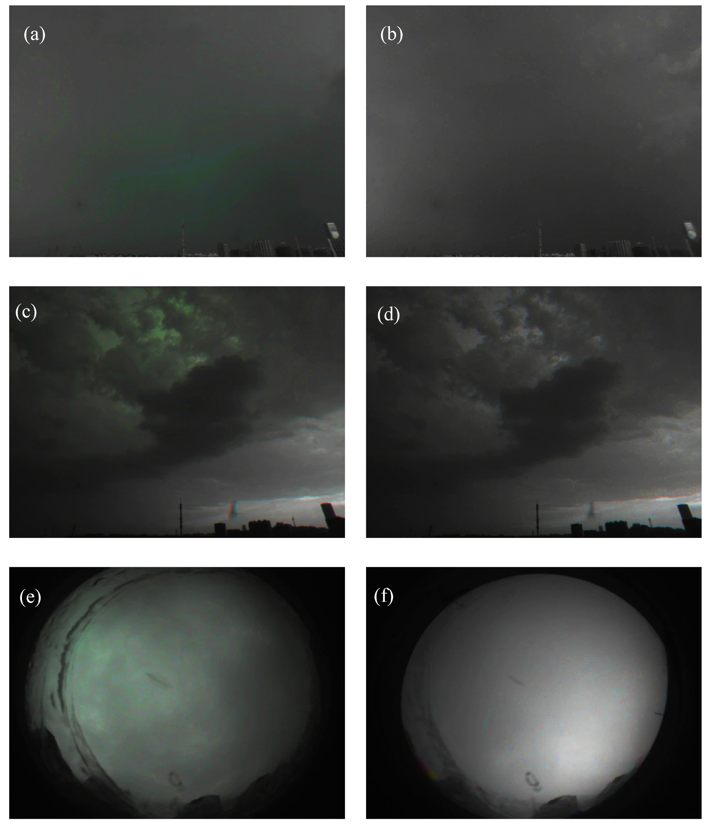
4.2. Comparison between Different Types of Cameras

A comparison between directional cameras and the all-sky camera was performed in ResNet152 during experiment 1. A total of 225 training epochs were performed, and the model weight checkpoint was recorded every 25 epochs. The loss profiles are plotted in Figure 10a, where the horizontal axis represents the number of epochs, and the vertical axis represents the loss. The curve corresponding to the all-sky camera has a bit of a quicker reducing speed, but the loss curves are both reduced to 0 as training proceeds.

For a general two-classification model with a given sample, the model outputs a corresponding score of S that is distributed from 0 to 1, where S = 1 indicates that the model considers this sample to be true with 100% credibility, while S = 0 indicates the opposite condition. If S is greater than the given threshold, then the sample is classified as true; otherwise, it is a false sample. By default, a threshold of 0.5 is used, but there may be a better threshold for a given task. Sliding the threshold from 0 to 1 gives different TRPs and FPRs, and ultimately, a receiver operating characteristic (ROC) curve is formed. For a 100% accurate classification model, this curve would be a broken line from (0,0) through (0,1) to (1,1). In other words, the closer the ROC is to the upper-left corner, the better the model’s classification.

Two checkpoints saved in the 150th epoch were tested in the test set. Figure 10b shows the ROC curves obtained for the test set using different cameras, and it can be seen that the curve corresponding to the all-sky camera is a bit closer to the upper-left corner, indicating that the classification results of the all-sky camera lightning images are slightly better using the same model. The results indicate that the distortion from the all-sky camera does not affect the recognition results.

4.3. Evaluation of the Preprocessing of the TSCs

The effect of using and not using the preprocessing of the TSCs was evaluated in ResNet152, ResNeXt101 (64 × 4d), Wide-ResNet101-2, and DenseNet161 during experiment 1. A total of 225 training epochs were performed, and the model weight checkpoint was recorded every 25 epochs. The loss profiles are plotted in Figure 11, where the horizontal axis represents the number of epochs, and the vertical axis represents the loss. It can be seen from the figure that regardless of the backbone used, the loss can converge to close to 0 after the 175th epoch after the TSCs are used, while the loss values without the usage of TSCs stabilize around 0.025, 0.004, 0.012, and 0.022 after the 100th epoch. It can be seen from the loss profiles that the classification performance of the model is significantly improved with the preprocessing of the TSCs, and the model can classify all the samples correctly in the training set after training, whereas without the preprocessing of the TSCs, the model is not even able to correctly classify all the samples in the training set.

Two checkpoints, the TSC-applied one saved at the 175th epoch and the non-TSC one saved at the 100th epoch, were extracted to perform predictions on the test set with a threshold of 0.5 for each model. A series of TPR and FPR values were obtained and are shown in

Table 3. Comparison of classification results on the test set with and without the preprocessing of TSC on the four models; a threshold of 0.5 is used.

	ResNet152		ResNeXt101 (64 × 4d)		WideResNet101-2		DenseNet161
	TPR (%)	FPR (%)	TPR (%)	FPR (%)	TPR (%)	FPR (%)	TPR (%)	FPR (%)
Not using TSC	53.4	3.1	54.9	3.5	51.6	2.1	58.4	3.0
Using TSC	93.0	0.8	91.7	0.8	93.4	0.8	91.6	1.0

. The TPR increases from 51~58% to 91~93%, and the FPR decreases from 2~3% to 0.8~1% after the preprocessing of the TSCs. Figure 12 shows the ROC curves obtained on the test set for the four backbones with and without the preprocessing of the TSCs. The ROC curves with the preprocessing of the TSCs are drastically bent to the upper-left corner, i.e., the model’s classification performance is significantly improved.

4.4. Comparison of Different Backbones

To determine the best backbone for the recognition of lightning images, ResNet152, ResNeXt101 (64 × 4), DenseNet161, and Wide-ResNet102-2 were used to train on the training set during experiment 1. A total of 225 training epochs were performed, and the model weight checkpoint was recorded every 25 epochs. The loss profiles obtained are plotted in Figure 13a. The difference in the decreasing trend in loss for different backbones can be seen, with ResNet152 being the slowest, ResNeXt101 (64 × 4) and Wide-ResNet101-2 being moderate, and DenseNet161 being the fastest; however, at the 175th epoch, the loss of all four backbones decreased to 0, approaching 100% accuracy on the training set.

The checkpoints saved at the 175th epoch were extracted separately and tested on the test set, and the ROC curves obtained are shown in Figure 13b, where the bolded line indicates the most effective DenseNet161. This task requires a high FPR, so the FPR is replaced by the number of false detections, and a logarithmic axis is used to represent it. The results show that DenseNet161 has the fastest loss decrease rate among all the backbones and the best performance on the test set.

The above results demonstrate that training with He-initialized DenseNet161 yields the best classifiers. The model weight checkpoints were saved every 25 epochs during the training process and tested separately on the test set to obtain the ROC curve, which is shown in Figure 14, where the bold line represents the 175th epoch of weights with the best results. Experiment 1 demands that the FPR be as low as possible; therefore, the FPR is replaced by the number of false detections and is represented using a logarithmic axis. The results show that the weights saved at the 175th epoch can guarantee both that the number of false detections is only 16 and that the recall rate is 86.5% when the threshold is 0.38, which satisfies the demand for the recognition of lightning images.

4.5. Recognition Results with a Higher Tolerability

DenseNet161, the best backbone in the previous experiment, was used in experiment 2 to perform the lightning image recognition task with a higher tolerability. A total of 255 training epochs were performed, and the model’s weight checkpoints were saved every 25 epochs. The loss profile obtained is shown in Figure 15a, where the horizontal axis is the number of epochs, and the vertical axis is the loss. The loss profile indicates that the loss stabilizes after 50 epochs and stabilizes close to 0.01. On the training set, the final model achieved a TPR of 99.9% and an FPR of 0.8%. Figure 15b shows the ROC curves obtained using the checkpoints saved every 25 epochs, where the bold lines are the weights of the 25th epoch with relatively good results. As shown in the figure, there cannot be a high TPR and a low number of false detections at the same time. If a high TPR is desired, the number of false detections will be more than one hundred, which is unacceptable. Although the model performs well on the training set, it does not perform well on the test set.

4.6. Summary of the Two Experiments

Table 4. Summary table of the two experiments.

		Experiment 1								Experiment 2
		ResNet152		ResNeXt (64 × 4d)		Wide-ResNet101-2		DenseNet161		DenseNet161
	Epoch	TPR (%)	NFP	TPR (%)	NFP	TPR (%)	NFP	TPR (%)	NFP	TPR (%)	NFP
Using TSCs	25	61.23	17	39.63	17	48.10	17	71.29	16	67.46	26
	50	72.39	17	80.74	17	77.67	17	78.53	24	6.22	26
	75	77.06	17	83.19	16	84.91	15	71.90	22	21.64	26
	100	85.15	17	75.71	17	83.93	17	73.37	24	27.98	26
	125	82.33	17	82.70	15	75.95	17	79.26	16	35.68	26
	150	79.75	16	80.86	17	80.61	17	80.37	16	24.36	26
	175	85.77	16	78.04	17	79.88	16	86.50	16	13.52	26
	200	81.35	17	78.40	17	79.63	17	80.74	16	27.15	26
	225	80.86	17	77.67	15	80.86	17	80.90	16	19.92	26
non- TSC	25	37.67	96	38.53	99	23.93	99	34.72	95
	50	31.29	96	37.18	98	42.33	96	35.83	99
	75	37.79	99	35.95	96	40.12	99	39.02	99
	100	34.72	98	36.56	99	35.46	99	35.95	99
	125	35.21	99	36.81	99	35.83	99	38.16	97
	150	37.55	99	34.48	99	35.71	95	38.77	99
	175	35.95	96	37.06	99	35.71	99	35.71	99
	200	36.44	98	38.28	99	35.21	96	39.63	99
	225	35.58	98	35.21	99	32.27	99	18.77	66

Bold corresponds to the best results for a particular backbone network in experiment 1, and underline corresponds to the best result in experiment 1.

lists all the results of the two experiments above. The checkpoints of every 25 epochs during training were tested in the test set. In experiment 1, an evaluation of the TSC method was performed in the four backbones, and the results are shown by the TPR and the number of false positives (NFP). It is obvious that the TPR using TSCs is 40% higher than the case not using TSCs, while the NFP is 80% lower. The best numbers for one backbone are bolded, and DenseNet161 in the 175th epoch reached a TPR of 86.5% and an NFP of 16, which is the best. In experiment 2, DenseNet161 is used to perform the recognition of harsher lightning images. The best case is in the 25th epoch, indicating that the model overfitted in later epochs. Although an NFP of 26 is considered low, a TPR of 67.46% is unacceptable.

5. Discussion

5.1. Incorrect Classification in Experiment 1

Two cases that indicate the reason for incorrect classification were identified in experiment 1, which are displayed in Figure 16.

The first case is the Bayes error rate, which was caused by the blurring of the classification boundary between the Weak and Blur types, i.e., the case in which the model could not classify the samples 100% correctly. Typical samples are shown in Figure 16a,b. Figure 16a shows a false positive sample, and Figure 16b shows a true negative sample. There is a green area in the cloud in both figures, which represents a light pulse in this area. The difference is that the luminous area in the “non-lightning” sample is smaller and weaker, whereas the luminous area in the “lightning” sample is stronger and larger. However, unclear classification boundaries inevitably occurred in a small number of manual labels, such as in Figure 16c,d, where the former is “non-lightning” and the latter is “lightning”, but the latter is slightly brighter than the former.

The second is the case where the morphology is similar and a human can perceive the difference, but the model still has difficulty recognizing it. As shown in Figure 16f, the Blur samples light up not only in the second frame but also in the first frame, which makes the whole picture appear yellowish green, resulting in a slight difference from the pure green Blur-type samples, which occupy a major part of the dataset. In addition, there are also some samples of a cyan color that are misclassified, and these samples light up in not only the second frame but also the third frame. Since the model can be put to practical use, the subsequent accumulation of training data is expected to solve the problem above. As shown in Figure 16h, the Clear-type samples only have the light-emitting channel showing gray-green, indicating that in the first and third frames, the channel is also lit up, so the change pattern between different frames is different from the general Clear samples, which is more like the None-type samples and easy to incorrectly classify. The incorrectly classified Living-type samples are shown in Figure 16e,g, where the former shows a bird rapidly passing by, which appears cyan, magenta, and yellow in the first, second, and third frames, respectively, and the latter shows a bird landing on an all-sky camera. Compared with Figure 16f, it can be seen from the picture that such a problem may be caused by the yellow area.

5.2. Incorrect Classification in Experiment 2

By analyzing the incorrectly classified samples in the training set and the test set, it is found that the trained model can easily recognize some “non-lightning” samples as “lightning” samples. Except for the Living type, these “non-lightning” samples have extremely similar “lightning” samples. Figure 17 displays three sets of comparisons after an 80% enhancement in saturation, where Figure 17a,c,e are the true positive “lightning” samples and Figure 17b,d,f are the false positive “non-lightning” samples. Obviously, the “lightning” sample still has a large green area, which represents the presence of a light pulse in the image, while the false positive “non-lightning” samples still have a gray color, which represents that there is no light pulse. These samples can be distinguished by the human eye, but they are difficult for the model to distinguish. This needs further research.

6. Conclusions

This paper collected lightning image data for five months at two optical observation stations and used a series of batch labeling methods to greatly reduce the workload of subsequent manual labeling, which established a lightning image dataset. The dataset contains more than 30,000 labeled samples, including three major categories of “strong lightning”, “weak lightning”, and “non-lightning” and five more detailed subcategories, with a considerable time span. Then, the TSC preprocessing method was proposed based on the significant time-varying characteristic of lightning, which can put the temporal features into the model while the model handles the spatial features to improve the model’s ability to recognize lightning. Two lightning image recognition experiments were performed, and the improvement in the ability to recognize lightning was evaluated on four backbones, including ResNet152, ResNeXt101 (64 × 4), DenseNet161, and Wide-ResNet102-2. Using DenseNet161 as the backbone, we can effectively classify “lightning” and “non-lightning”, and the number of false detections was only 16, with an 86.5% recall rate, which can support automatic lightning image recognition. However, there is still a problem with the second experiment attempted in this paper, which puts Weak-type samples under “lightning”, so we aim to further improve the detection efficiency. The results show that the model is prone to false detections due to the problem of samples being too close to each other during classification, which requires further research.

References

1. Qie, X.; Kong, X. Progression Features of a Stepped Leader Process with Four Grounded Leader Branches. Geophys. Res. Lett. 2007, 34. [Google Scholar] [CrossRef]
2. Qie, X.; Wang, Z.; Wang, D.; Liu, M. Characteristics of Positive Cloud-to-Ground Lightning in Da Hinggan Ling Forest Region at Relatively High Latitude, Northeastern China. J. Geophys. Res. Atmos. 2013, 118, 13393–13404. [Google Scholar] [CrossRef]
3. Qie, X.; Jiang, R.; Wang, C.; Yang, J.; Wang, J.; Liu, D. Simultaneously Measured Current, Luminosity, and Electric Field Pulses in a Rocket-Triggered Lightning Flash. J. Geophys. Res. Atmos. 2011, 116, D10102. [Google Scholar] [CrossRef]
4. Qie, X.; Zhang, Q.; Zhou, Y.; Feng, G.; Zhang, T.; Yang, J.; Kong, X.; Xiao, Q.; Wu, S. Artificially Triggered Lightning and Its Characteristic Discharge Parameters in Two Severe Thunderstorms. Sci. China Ser. Earth Sci. 2007, 50, 1241–1250. [Google Scholar] [CrossRef]
5. Qie, X.; Pu, Y.; Jiang, R.; Sun, Z.; Liu, M.; Zhang, H.; Li, X.; Lu, G.; Tian, Y. Bidirectional Leader Development in a Preexisting Channel as Observed in Rocket-Triggered Lightning Flashes. J. Geophys. Res. Atmos. 2017, 122, 586–599. [Google Scholar] [CrossRef]
6. Qie, X.; Zhao, Y.; Zhang, Q.; Yang, J.; Feng, G.; Kong, X.; Zhou, Y.; Zhang, T.; Zhang, G.; Zhang, T.; et al. Characteristics of Triggered Lightning during Shandong Artificial Triggering Lightning Experiment (SHATLE). Atmos. Res. 2009, 91, 310–315. [Google Scholar] [CrossRef]
7. Qie, X.; Zhang, T.; Chen, C.; Zhang, G.; Zhang, T.; Wei, W. The Lower Positive Charge Center and Its Effect on Lightning Discharges on the Tibetan Plateau. Geophys. Res. Lett. 2005, 32, L05814. [Google Scholar] [CrossRef]
8. Qie, X.; Wu, X.; Yuan, T.; Bian, J.; Lu, D. Comprehensive Pattern of Deep Convective Systems over the Tibetan Plateau–South Asian Monsoon Region Based on TRMM Data. J. Clim. 2014, 27, 6612–6626. [Google Scholar] [CrossRef]
9. Qie, X.; Toumi, R.; Yuan, T. Lightning Activities on the Tibetan Plateau as Observed by the Lightning Imaging Sensor. J. Geophys. Res. Atmos. 2003, 108, 4551. [Google Scholar] [CrossRef]
10. Qie, X.; Qie, K.; Wei, L.; Zhu, K.; Sun, Z.; Yuan, S.; Jiang, R.; Zhang, H.; Xu, C. Significantly Increased Lightning Activity Over the Tibetan Plateau and Its Relation to Thunderstorm Genesis. Geophys. Res. Lett. 2022, 49, e2022GL099894. [Google Scholar] [CrossRef]
11. Kohlmann, H.; Schulz, W.; Pedeboy, S. Evaluation of EUCLID IC/CG Classification Performance Based on Ground-Truth Data. In Proceedings of the 2017 International Symposium on Lightning Protection (XIV SIPDA), Natal, Brazil, 2–6 October 2017; pp. 35–41. [Google Scholar] [CrossRef]
12. Schonland, B.F.J.; Collens, H. Progressive Lightning. Trans. S. Afr. Inst. Electr. Eng. 1934, 25, 124–135. [Google Scholar]
13. Yokoyama, S.; Miyake, K.; Suzuki, T.; Kanao, S. Winter Lightning on Japan Sea Coast-Development of Measuring System on Progressing Feature of Lightning Discharge. IEEE Trans. Power Deliv. 1990, 5, 1418–1425. [Google Scholar] [CrossRef]
14. Jiang, R.; Wu, Z.; Qie, X.; Wang, D.; Liu, M. High-Speed Video Evidence of a Dart Leader with Bidirectional Development. Geophys. Res. Lett. 2014, 41, 5246–5250. [Google Scholar] [CrossRef]
15. Pu, Y.; Qie, X.; Jiang, R.; Sun, Z.; Liu, M.; Zhang, H. Broadband Characteristics of Chaotic Pulse Trains Associated With Sequential Dart Leaders in a Rocket-Triggered Lightning Flash. J. Geophys. Res.-Atmos. 2019, 124, 4074–4085. [Google Scholar] [CrossRef]
16. Jiang, R.; Srivastava, A.; Qie, X.; Yuan, S.; Zhang, H.; Sun, Z.; Wang, D.; Wang, C.; Lv, G.; Li, Z. Fine Structure of the Breakthrough Phase of the Attachment Process in a Natural Lightning Flash. Geophys. Res. Lett. 2021, 48, e2020GL091608. [Google Scholar] [CrossRef]
17. Sun, Z.; Qie, X.; Jiang, R.; Liu, M.; Wu, X.; Wang, Z.; Lu, G.; Zhang, H. Characteristics of a Rocket-Triggered Lightning Flash with Large Stroke Number and the Associated Leader Propagation. J. Geophys. Res. Atmos. 2014, 119, 13388–13399. [Google Scholar] [CrossRef]
18. Wang, C.-X.; Qie, X.-S.; Jiang, R.-B.; Yang, J. Propagating properties of a upward positive leader in a negative triggered lightning. ACTA Phys. Sin. 2012, 61, 039203. [Google Scholar] [CrossRef]
19. Wang, Z.; Qie, X.; Jiang, R.; Wang, C.; Lu, G.; Sun, Z.; Liu, M.; Pu, Y. High-Speed Video Observation of Stepwise Propagation of a Natural Upward Positive Leader. J. Geophys. Res. Atmos. 2016, 121, 14307–14315. [Google Scholar] [CrossRef]
20. Kong, X.; Qie, X.; Zhao, Y. Characteristics of Downward Leader in a Positive Cloud-to-Ground Lightning Flash Observed by High-Speed Video Camera and Electric Field Changes. Geophys. Res. Lett. 2008, 35, L05816. [Google Scholar] [CrossRef]
21. Chen, L.; Lu, W.; Zhang, Y.; Wang, D. Optical Progression Characteristics of an Interesting Natural Downward Bipolar Lightning Flash. J. Geophys. Res. Atmos. 2015, 120, 708–715. [Google Scholar] [CrossRef]
22. Lu, W.; Chen, L.; Zhang, Y.; Ma, Y.; Gao, Y.; Yin, Q.; Chen, S.; Huang, Z.; Zhang, Y. Characteristics of Unconnected Upward Leaders Initiated from Tall Structures Observed in Guangzhou. J. Geophys. Res. Atmos. 2012, 117, D19211. [Google Scholar] [CrossRef]
23. Lu, W.; Wang, D.; Takagi, N.; Rakov, V.; Uman, M.; Miki, M. Characteristics of the Optical Pulses Associated with a Downward Branched Stepped Leader. J. Geophys. Res. Atmos. 2008, 113, D21206. [Google Scholar] [CrossRef]
24. Lu, W.; Wang, D.; Zhang, Y.; Takagi, N. Two Associated Upward Lightning Flashes That Produced Opposite Polarity Electric Field Changes. Geophys. Res. Lett. 2009, 36, L05801. [Google Scholar] [CrossRef]
25. Lu, W.; Chen, L.; Ma, Y.; Rakov, V.A.; Gao, Y.; Zhang, Y.; Yin, Q.; Zhang, Y. Lightning Attachment Process Involving Connection of the Downward Negative Leader to the Lateral Surface of the Upward Connecting Leader. Geophys. Res. Lett. 2013, 40, 5531–5535. [Google Scholar] [CrossRef]
26. Gao, Y.; Lu, W.; Ma, Y.; Chen, L.; Zhang, Y.; Yan, X.; Zhang, Y. Three-Dimensional Propagation Characteristics of the Upward Connecting Leaders in Six Negative Tall-Object Flashes in Guangzhou. Atmos. Res. 2014, 149, 193–203. [Google Scholar] [CrossRef]
27. Lu, W.; Zhang, Y.; Zhou, X.; Qie, X.; Zheng, D.; Meng, Q.; Ma, M.; Chen, S.; Wang, F.; Kong, X. Simultaneous Optical and Electrical Observations on the Initial Processes of Altitude-Triggered Negative Lightning. Atmos. Res. 2009, 91, 353–359. [Google Scholar] [CrossRef]
28. Zhou, E.; Lu, W.; Zhang, Y.; Zhu, B.; Zheng, D.; Zhang, Y. Correlation Analysis between the Channel Current and Luminosity of Initial Continuous and Continuing Current Processes in an Artificially Triggered Lightning Flash. Atmos. Res. 2013, 129–130, 79–89. [Google Scholar] [CrossRef]
29. Wang, J.; Su, R.; Wang, J.; Wang, F.; Cai, L.; Zhao, Y.; Huang, Y. Observation of Five Types of Leaders Contained in a Negative Triggered Lightning. Sci. Rep. 2022, 12, 6299. [Google Scholar] [CrossRef]
30. Cai, L.; Chu, W.; Zhou, M.; Su, R.; Xu, C.; Wang, J.; Fan, Y. Observation and Modeling of Attempted Leaders in a Multibranched Altitude-Triggered Lightning Flash. IEEE Trans. Electromagn. Compat. 2023, 65, 1133–1142. [Google Scholar] [CrossRef]
31. Winckler, J.R.; Malcolm, P.R.; Arnoldy, R.L.; Burke, W.J.; Erickson, K.N.; Ernstmeyer, J.; Franz, R.C.; Hallinan, T.J.; Kellogg, P.J.; Monson, S.J.; et al. ECHO 7: An Electron Beam Experiment in the Magnetosphere. Eos Trans. Am. Geophys. Union 1989, 70, 657–668. [Google Scholar] [CrossRef]
32. Pasko, V.P.; Stanley, M.A.; Mathews, J.D.; Inan, U.S.; Wood, T.G. Electrical Discharge from a Thundercloud Top to the Lower Ionosphere. Nature 2002, 416, 152–154. [Google Scholar] [CrossRef] [PubMed]
33. Soula, S.; van der Velde, O.; Montanyà, J.; Neubert, T.; Chanrion, O.; Ganot, M. Analysis of Thunderstorm and Lightning Activity Associated with Sprites Observed during the EuroSprite Campaigns: Two Case Studies. Atmos. Res. 2009, 91, 514–528. [Google Scholar] [CrossRef]
34. Yang, J.; Lu, G.; Liu, N.; Cui, H.; Wang, Y.; Cohen, M. Analysis of a Mesoscale Convective System That Produced a Single Sprite. Adv. Atmos. Sci. 2017, 34, 258–271. [Google Scholar] [CrossRef]
35. Wang, X.; Wang, H.; Lyu, W.; Chen, L.; Ma, Y.; Qi, Q.; Wu, B.; Xu, W.; Hua, L.; Yang, J.; et al. First Experimental Verification of Opacity for the Lightning Near-Infrared Spectrum. Geophys. Res. Lett. 2022, 49, e2022GL098883. [Google Scholar] [CrossRef]
36. Wan, R.; Yuan, P.; An, T.; Liu, G.; Wang, X.; Wang, W.; Huang, X.; Deng, H. Effects of Atmospheric Attenuation on the Lightning Spectrum. J. Geophys. Res. Atmos. 2021, 126, e2021JD035387. [Google Scholar] [CrossRef]
37. Lecun, Y.; Bottou, L.; Bengio, Y.; Haffner, P. Gradient-Based Learning Applied to Document Recognition. Proc. IEEE 1998, 86, 2278–2324. [Google Scholar] [CrossRef]
38. Krizhevsky, A.; Sutskever, I.; Hinton, G.E. ImageNet Classification with Deep Convolutional Neural Networks. In Advances in Neural Information Processing Systems; Curran Associates, Inc.: New York, NY, USA, 2012; Volume 25. [Google Scholar]
39. Szegedy, C.; Liu, W.; Jia, Y.; Sermanet, P.; Reed, S.; Anguelov, D.; Erhan, D.; Vanhoucke, V.; Rabinovich, A. Going Deeper with Convolutions. In Proceedings of the 2015 IEEE Conference on Computer Vision and Pattern Recognition (CVPR), Boston, MA, USA, 7–12 June 2015; pp. 1–9. [Google Scholar] [CrossRef]
40. He, K.; Zhang, X.; Ren, S.; Sun, J. Deep Residual Learning for Image Recognition. In Proceedings of the 2016 IEEE Conference on Computer Vision and Pattern Recognition (CVPR), Las Vegas, NV, USA, 27–30 June 2016; pp. 770–778. [Google Scholar] [CrossRef]
41. Zagoruyko, S.; Komodakis, N. Wide Residual Networks. arXiv 2017, arXiv:1605.07146. [Google Scholar]
42. Xie, S.; Girshick, R.; Dollár, P.; Tu, Z.; He, K. Aggregated Residual Transformations for Deep Neural Networks. In Proceedings of the 2017 IEEE Conference on Computer Vision and Pattern Recognition (CVPR), Honolulu, HI, USA, 21–26 July 2017; pp. 5987–5995. [Google Scholar] [CrossRef]
43. Huang, G.; Liu, Z.; Van Der Maaten, L.; Weinberger, K.Q. Densely Connected Convolutional Networks. In Proceedings of the 2017 IEEE Conference on Computer Vision and Pattern Recognition (CVPR), Honolulu, HI, USA, 21–26 July 2017; pp. 2261–2269. [Google Scholar] [CrossRef]
44. Zhao, B.; Li, X.; Lu, X.; Wang, Z. A CNN-RNN Architecture for Multi-Label Weather Recognition. Neurocomputing 2018, 322, 47–57. [Google Scholar] [CrossRef]
45. Lv, Q.; Li, Q.; Chen, K.; Lu, Y.; Wang, L. Classification of Ground-Based Cloud Images by Contrastive Self-Supervised Learning. Remote Sens. 2022, 14, 5821. [Google Scholar] [CrossRef]
46. He, K.; Zhang, X.; Ren, S.; Sun, J. Delving Deep into Rectifiers: Surpassing Human-Level Performance on ImageNet Classification. In Proceedings of the 2015 IEEE International Conference on Computer Vision (ICCV), Santiago, Chile, 7–13 December 2015; pp. 1026–1034. [Google Scholar] [CrossRef]
Figure 1. Sample of lightning images. (a) Lightning at night. (b) Lightning in the daytime. (c) Lightning obscured by clouds. (d) Lightning partially obscured by clouds recorded using an all-sky camera.
Remotesensing 16 01151 g001
Figure 2. Batch labeling method flowchart.
Remotesensing 16 01151 g002
Figure 3. Schematic diagram of the preprocessing method of a time sequence composite (TSC).
Remotesensing 16 01151 g003
Figure 4. Four examples of preprocessed samples. (a) Lightning that only lights up 1 frame. (b) Lightning that lights up over 3 frames. (c) Lightning in a cloud that lights up in a different area. (d) A bird landing on camera.
Remotesensing 16 01151 g004
Figure 5. Dataset categories displayed in timeline form and TSC form.
Remotesensing 16 01151 g005
Figure 6. (a) The number of different types of samples over time. (b) Distribution of the average brightness of different types of samples. (c) Distribution of the average saturation of different types of samples. (d) Distribution of the maximum saturation of different types of samples.
Remotesensing 16 01151 g006
Figure 7. Division of positive and negative examples from the two experiments.
Remotesensing 16 01151 g007
Figure 8. Distribution of the number of remaining unlabeled video files after labeling with FQ1 and FQ2; the date is formatted as dd/mm/yyyy.
Remotesensing 16 01151 g008
Figure 9. Distribution of the count of occurrences of light pulses in every single file.
Remotesensing 16 01151 g009
Figure 10. Comparison between different cameras. (a) Loss curve; (b) ROC.
Remotesensing 16 01151 g010
Figure 11. Comparison of loss profiles with and without the preprocessing of TSCs. (a) ResNet152. (b) ResNeXt101 (64 × 4d). (c) WideResNet101-2. (d) DenseNet161.
Remotesensing 16 01151 g011
Figure 12. Comparison of receiver operating characteristic (ROC) curves with and without the preprocessing of TSCs.
Remotesensing 16 01151 g012
Figure 13. (a) Comparison of loss profiles using different backbones. (b) Comparison of ROC curves obtained during testing on the test set using different backbones.
Remotesensing 16 01151 g013
Figure 14. Comparison of ROC curves obtained from different checkpoints saved at different epochs.
Remotesensing 16 01151 g014
Figure 15. (a) The loss profile. (b) Comparison of ROC curves obtained from different checkpoints saved at different epochs.
Remotesensing 16 01151 g015
Figure 16. Display of incorrectly classified samples. (a) False positive sample, Weak-type. (b) True negative sample, Blur-type. (c) False positive sample, Weak-type. (d) True negative sample, Blur-type. (e) False positive sample, Living-type. (f) True negative sample, Blur-type. (g) False positive sample, Living-type. (h) True negative sample, Clear-type.
Remotesensing 16 01151 g016aRemotesensing 16 01151 g016b
Figure 17. Comparison of similar Weak- and None-type samples: the saturation of all samples was enhanced by 80%. (a) A true positive sample, Weak-type. (b) A false positive sample, None-type. (c) A true positive sample, Weak-type. (d) A false positive sample, None-type. (e) A true positive sample, Weak-type. (f) A false positive sample, None-type.
Remotesensing 16 01151 g017