Automated Estimation of Sub-Canopy Topography Combined with Single-Baseline Single-Polarization TanDEM-X InSAR and ICESat-2 Data

Abstract

TanDEM-X bistatic interferometric system successfully generated a high-precision, high-resolution global digital elevation model (DEM). However, in forested areas, two core problems make it difficult to obtain sub-canopy topography: (1) the penetrability of short-wave signals is limited, and the DEM obtained in dense forest areas contains a significant forest signal, that is, the scattering phase center (SPC) height; and (2) the single-baseline and single-polarization TanDEM-X interferometric synthetic aperture radar (InSAR) data cannot provide sufficient observations to make the existing physical model reversible for estimating the real surface phase, whereas the introduction of optical data makes it difficult to ensure data synchronization and availability of cloud-free data. To overcome these problems in accurately estimating sub-canopy topography from TanDEM-X InSAR data, this study proposes a practical method of sub-canopy topography estimation based on the following innovations: (1) An orthogonal polynomial model was established using TanDEM-X interferometric coherence and slope to estimate the SPC height. Interferometric coherence records forest height and dielectric property information from an InSAR perspective and has spatiotemporal consistency with the InSAR-derived DEM. (2) Introduce Ice, Cloud, and Land Elevation Satellite-2 (ICESat-2) data to provide more observational information and automatically screen ICESat-2 control points with similar forest and slope conditions in the local area to suppress forest spatial heterogeneity. (3) A weighted least squares criterion was used to solve this model to estimate the SPC height. The results were validated at four test sites using high-precision airborne light detection and ranging (LiDAR) data as a reference. Compared to the InSAR-derived DEM, the accuracy of the sub-canopy topography was improved by nearly 60%, on average. Furthermore, we investigated the necessity of local modeling, confirming the potential of the proposed method for estimating sub-canopy topography by relying only on TanDEM-X and ICESat-2 data.

1. Introduction

Digital elevation models (DEMs) are indispensable data sources for natural resource investigations, disaster monitoring, and climate and ecological change analyses [1,2]. With the development of the economy and society, higher requirements have been proposed for large-scale, high-precision, and high-spatial-resolution DEMs. For this purpose, interferometric synthetic aperture radar (InSAR) is widely used for DEM extraction [2,3,4] and is considered to be a favorable tool for global DEM acquisition and updating because of its spatial continuity and independence from weather conditions [5,6].

TanDEM-X, the first twin-satellite spaceborne interferometric system, has been successfully used to acquire a global DEM with a resolution of 12 m [2,7,8]. However, owing to its limited penetrability, the DEM obtained from TanDEM-X InSAR data contains significant forest height signals [9]. Consequently, the obtained DEM does not reflect sub-canopy topography, which is important for many applications. Therefore, it is necessary to remove the forest height signals from TanDEM-X InSAR-derived DEM.

To obtain a high-precision sub-canopy topography, methods based on polarimetric InSAR (PolInSAR) have been extensively developed [10,11,12]. Among them, the random volume over ground (RVoG) model has been widely used to describe the scattering induced by forests and this can be utilized to distinguish forest and ground scattering contributions in a common resolution cell [13,14]. In addition, methods based on sub-aperture [15] and tomographic SAR (TomoSAR) [16,17,18] have been used to remove vegetation signals from the InSAR-derived DEM. Such methods do not depend on any scattering model and use only InSAR observations without any external data. However, they require multi-baseline, multi-polarization, time–frequency, or long–wave SAR data. Therefore, these methods cannot be applied to standard TanDEM-X InSAR data, owing to the limited number of interferometric pairs, single polarization, and poor penetrability.

The goal of estimating large-scale sub-canopy topography was typically achieved by estimating forest stand heights at their boundaries and subtracting average values from the InSAR-derived DEM [19]. However, forest boundary height does not truly represent the height of the entire forest. To overcome this limitation, some studies have suggested employing external data acquired by spaceborne LiDAR systems [20,21,22,23], including the Ice, Cloud, and Land Elevation Satellite (ICESat) and the Global Ecosystem Dynamics Investigation (GEDI). There are two methods for obtaining sub-canopy topography by introducing spaceborne LiDAR data: (1) using forest heights obtained by the spaceborne LiDAR satellite combined with multi-source remote sensing data to estimate forest height, and then removing the forest signal in the InSAR-derived DEM in proportion [9,21,23,24]. Alternatively, Wang et al. estimated the penetration depth of the InSAR signal based on the infinite depth hypothesis model and established a relationship between forest height and penetration depth to obtain the sub-canopy topography [9]. Unfortunately, the synchronization of InSAR, spaceborne LiDAR, and other remote sensing data is difficult to guarantee, leading to great uncertainty in forest dynamic change areas. (2) Using spaceborne LiDAR ground elevation as a reference, combined with parameters for optical characteristics for regression analysis to train and predict the scattering phase center (SPC) height, and then the SPC height is subtracted from the InSAR-derived DEM to obtain sub-canopy topography [20,22,25,26,27,28]. However, it is difficult to guarantee consistency of the temporal and spatial resolutions of these optical variables. More importantly, introducing optical data to estimate SPC height may have limitations related to the availability of cloudless data, spatial heterogeneity of forest attributes, and lack of sensitivity to forest density in tall and dense forests [29].

To overcome these limitations, this study combines the following innovations and proposes a framework for estimating sub-canopy topography:

(1)

Modeling to estimate SPC height using only the interferometric coherence and slope obtained from TanDEM-X InSAR data. Compared with optical parameters, TanDEM-X InSAR interferometric coherence records the scattering process of InSAR signals in the forest and is sensitive to forest height, vertical structure, and dielectric properties. More importantly, it exhibits time synchronization and consistency in spatial resolution with the InSAR-derived DEM.

(2)

ICESat-2 terrain control points (TCPs) with similar forest and slope conditions were adaptively screened within a local area to establish the model. The highlight of the framework for the estimation of SPC height is that the screening strategy comprehensively considers the spatial heterogeneity of forest characteristics and the influence of slope. In addition, the adaptive selection of TCPs enables the framework to estimate the SPC height well when ICESat-2 data are sparse.

(3)

A weighted least-squares criterion was used to solve the model to estimate the SPC height, which can adapt to the influence on the results of different distances of the ICESat-2 TCPs.

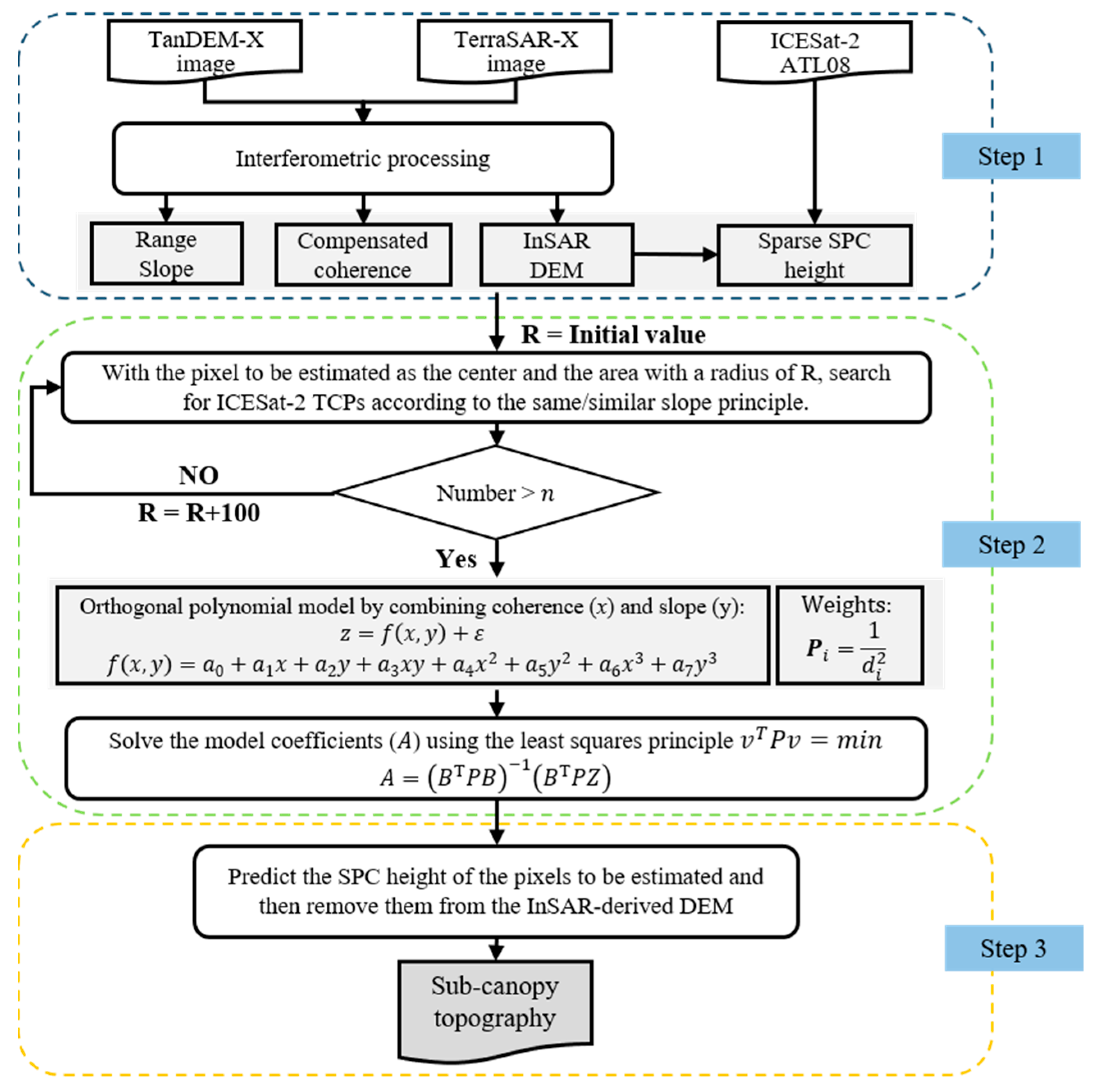
The remainder of this paper is organized as follows. Section 2 describes the proposed framework for sub-canopy topography estimation. Section 3 describes the study area and the available experimental data. In Section 4, the effectiveness of this method is tested using single-polarization and baseline TanDEM-X InSAR data from four test sites with different topographies and forest conditions. Section 5 further discusses the results of sub-canopy topography estimation. Finally, our conclusions are presented in Section 6.

2. Methods

The purpose of this study was to estimate high-precision sub-canopy topography by combining TanDEM-X InSAR data and ICESat-2 TCPs. The method proposed correlates elevation differences (i.e., SPC height) from ICESat-2/InSAR-derived DEMs with interferometric coherence and slope. The overall flowchart of the algorithm is shown in Figure 1.

The first step was to obtain a high-precision InSAR-derived DEM and corrected coherence through interferometric processing of the TanDEM-X InSAR data. Simultaneously, InSAR-derived DEM, interferometric coherence, and slope were matched to the closest ICESat-2 orbital geodetic (latitude and longitude) locations. The second step considered the influence of interferometric coherence and slope on SPC height to model and obtained sufficient TCPs through the screening strategy to solve the model coefficients using the least squares criterion ($v^{T}Pv=min$). The second step is key in the proposed method to estimate the sub-canopy topography and highlight the innovative contribution of the proposed method, which is described in detail in the following sections. The third step is to predict the SPC height of a specified pixel and remove it from the InSAR-derived DEM to obtain the sub-canopy topography.

2.1. Scattering Phase Center Height Retrieval Algorithm

The TanDEM-X system can simultaneously acquire two complex SAR images, $S_1$ and $S_2$, and perform interferometry as follows [30]:

$$\gamma =\frac{⟨S_1\cdot S_2^{*}⟩}{\sqrt{⟨{\left|S_1\right|}^2⟩\cdot ⟨{\left|S_2\right|}^2⟩}}$$

(1)

where $⟨·⟩$ represents expectation operation, $\gamma$ is the complex interferometric coherence. In forested areas, although $\gamma$ is not affected by temporal decorrelation, many sources of decorrelation still reduce interferometric coherence [30,31]. Among them, the decorrelation associated with the SAR sensor parameters, acquisition geometry, thermal noise, and quantization errors can be canceled or minimized using known specific strategies [6,32,33]. Therefore, the compensated interferometric coherence directly manifests as volume decorrelation, which is related to forest height, vertical structure, and dielectric properties and is an important parameter for the estimation of SPC height. The interferometric coherence subsequently used for modeling in this study refers to the volume decorrelation after compensation.

The interferometric phase was used to estimate DEM [9,34], but in forested areas, the InSAR-derived DEM cannot represent the real surface elevation [20,35]. As shown in Figure 2, in mountainous areas covered by vegetation, the distance D was affected by forest height and terrain slope. Owing to the influence of the forest, the actual distance Dr of the TanDEM-X InSAR signal propagation was shorter than D (Figure 2a). This part is the SPC height caused by forest volume scattering. In addition, as shown in Figure 2b,c, when there is terrain slope α of the ground surface, the slope causes the distance D to increase or decrease. A larger slope will further increase the change in D [20,36,37], which will affect the accuracy of obtaining the sub-canopy topography using InSAR technology.

In conclusion, the SPC height is related to forest volume scattering and is determined by the forest height, forest density, and dielectric properties [22,38,39]. In other words, the SPC height can be linked to interferometric coherence [13,14,40]. In addition, the slope is also a key factor affecting the SPC height. However, single-baseline and single-polarization TanDEM-X data acquired in standard mode makes it difficult to satisfy the existing physical models (e.g., random volume over ground, RVoG) to estimate the SPC height. Fortunately, spaceborne LiDAR systems (e.g., ICESat-2), although they have a low spatial resolution, can estimate some SPC heights from TanDEM-X InSAR data. Using the sparse SPC heights, a multi-regression model can be produced with the form:

$$\begin{array}{c}z=f\left(x,y\right)+\epsilon \\ f\left(x,y\right)=a_0+a_{1}x+a_{2}y+{a_{3}xy+a}_4{x}^2+a_5{y}^2+a_6{x}^3+a_7{y}^3\end{array}$$

(2)

where $z$ is the real SPC height, $\epsilon$ is the fitting residual, $f\left(x,y\right)$ is the SPC height of the polynomial fitting, $a_i$ ($i$ = 0, 1, ⋯, 7) is the polynomial coefficient, $x$ represents the interferometric coherence, $y$ represents the slope. The slope (derived from the TanDEM DEM) represents the terrain slope in the range direction and is positive when facing toward the SAR satellite.

2.2. Estimation of the SPC Height

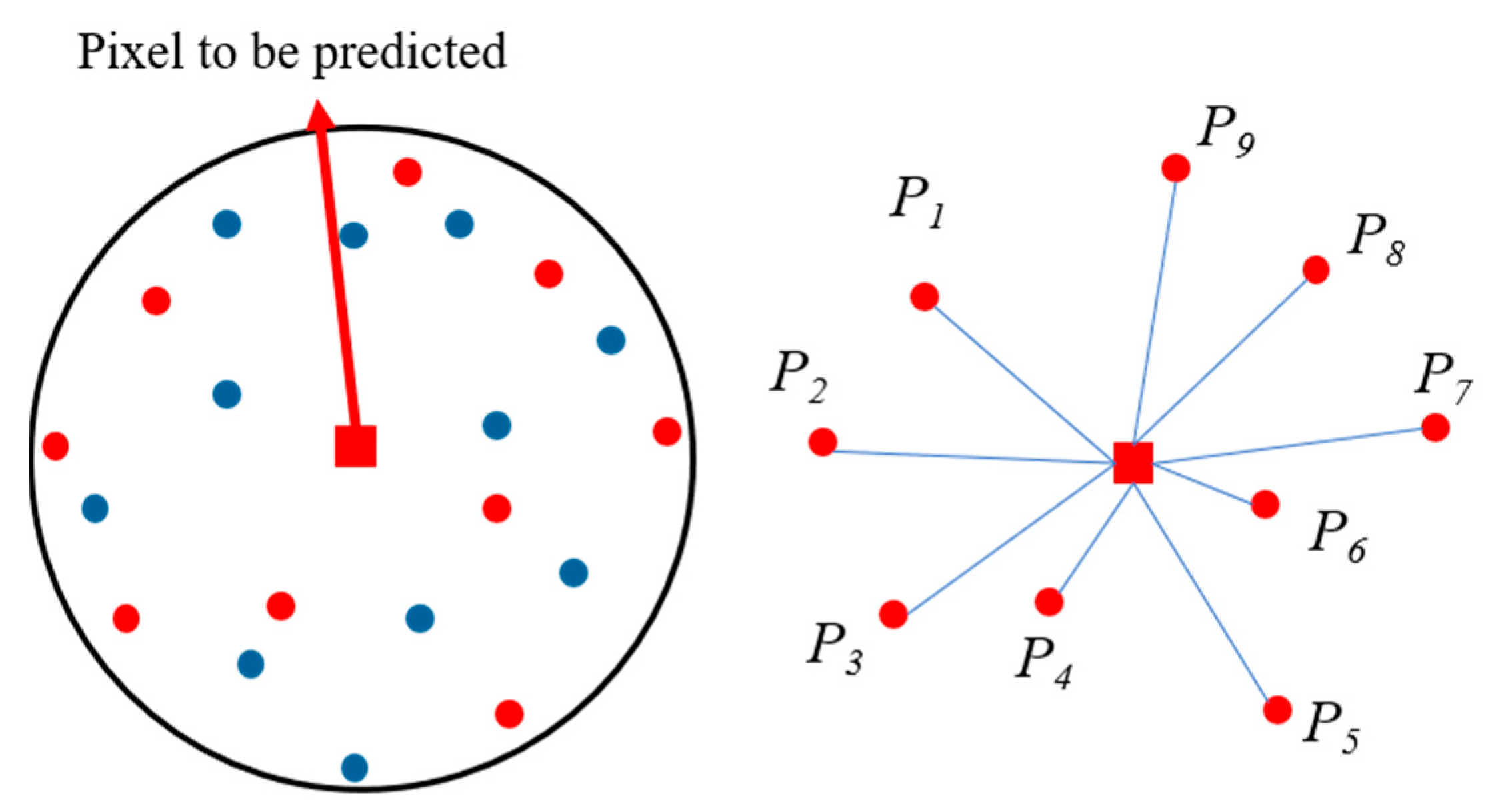
This model solution requires sufficient ICESat-2 TCPs to improve robustness. For the entire SAR image, the existing regression analysis strategy uses all screened ICESat-2 TCPs to fit and solve a set of coefficients to predict the SPC height of the ICESat-2 uncovered area [20,22,26]. However, in many cases, it is difficult to predict the SPC height using interferometric coherence because the same interferometric coherence can be measured in forests with different vertical structures and dielectric properties. That is, the same interferometric coherence may correspond to different SPC heights. Therefore, to estimate SPC height more accurately, the orthogonal model applies a local fitting strategy and selects similar ICESat-2 TCPs for any pixel to fit and predict SPC height.

As shown in Figure 3, the red rectangle represents the pixel within which SPC height is to be predicted, and the dot with the same color (red) represents the ICESat-2 TCPs used for fitting. The ICESat-2 TCPs were selected for fitting based on the following two conditions:

(1)

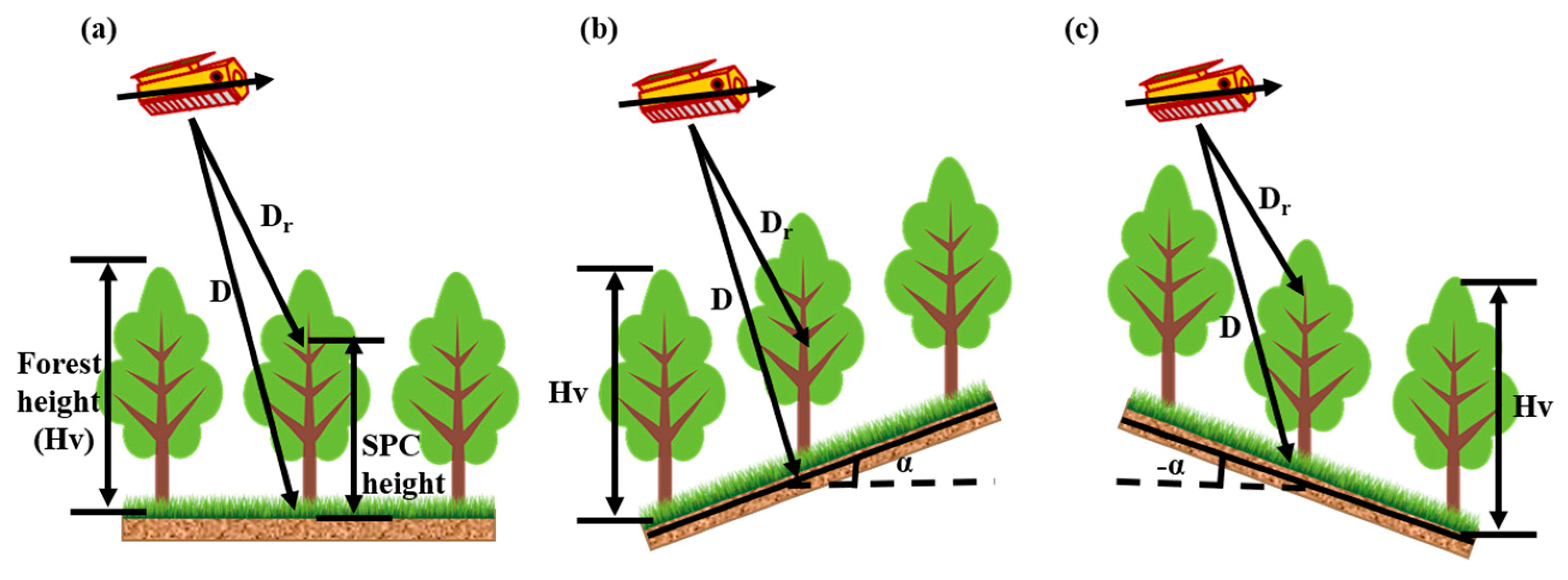
Condition 1: Search within a local circular area with the pixel to be predicted as the center and R as the radius. The initial value of R can be empirically set based on the existing coverage density of ICESat-2, which is 100 pixels in this study. We assumed that forest conditions (i.e., type, density, and dielectric properties) were the same or similar within a local area. When the slope is zero, different interferometric coherences correspond to different SPC heights.

(2)

Condition 2: Based on Condition 1, ICESat-2 TCPs with the same slope direction (positive or negative) were selected to solve the orthogonal polynomial model. As shown in Figure 2, when a certain terrain slope exists, it leads to a higher or lower SPC height at the same geographical location [20]. In addition, the slope distorts the relationship between interferometric coherence and SPC height. In the positive slope area, the interferometric coherence decreased with an increase in slope, because the increase in slope leads to an increase in volume scattering caused by the forest canopy in the same forest environment [41]. Conversely, in the negative slope area, the increase in slope increases the surface scattering that occurs at the top of the forest, whereas the volumetric scattering caused by the forest canopy decreases. Therefore, this selection condition was beneficial for avoiding the heterogeneity caused by different slope directions to better predict the SPC height.

Figure 3. Schematic diagram of ICESat-2 TCPs selection and weighting scheme. The red rectangle is the pixel of the height of the SPC to be predicted. The dots represent the ICESat-2 footprint points, where red indicates control points with the same/similar forests and terrain as the pixels to be predicted, and blue indicates control points that do not participate in the modeling.

Figure 3. Schematic diagram of ICESat-2 TCPs selection and weighting scheme. The red rectangle is the pixel of the height of the SPC to be predicted. The dots represent the ICESat-2 footprint points, where red indicates control points with the same/similar forests and terrain as the pixels to be predicted, and blue indicates control points that do not participate in the modeling.

Based on the above two conditions, for each pixel whose SPC height was to be predicted, $n$ ICESat-2 TCPs were selected for modeling using an iterative method. The least-squares criterion was then used to solve the coefficients of the model [42,43], and the following equations can be obtained from the values of $n$ (e.g., 30) ICESat-2 TCPs:

$$\underset{n\times 1}{v}=\underset{n\times 8}{\mathit{B}}\cdot \underset{8\times 1}{\mathrm{A}}+\underset{n\times 1}{Z}$$

(3)

The matrix form of each can be expressed as follows:

$$v=\left[\begin{array}{c}{V}_1\\ V_2\\ ⋮\\ V_n\end{array}\right],B=\left[\begin{array}{cccccccc}1& x_1& y_1& x_1{y}_1& x_1^2& y_1^2& x_1^3& y_1^3\\ 1& x_2& y_2& x_2{y}_2& x_2^2& y_2^2& x_2^3& y_2^3\\ ·& ·& ·& ·& ·& ·& ·& ·\\ 1& x_n& y_n& x_n{y}_n& x_n^2& y_n^2& x_n^3& y_n^3\end{array}\right], A=\left[\begin{array}{c}{a}_0\\ a_2\\ ⋮\\ a_7\end{array}\right],Z=\left[\begin{array}{c}{Z}_1\\ Z_2\\ ⋮\\ Z_n\end{array}\right]$$

(4)

According to Formula (4) and the principle of least squares $v^{T}Pv=min$, the values of the parameter $a_i$ ($i$ = 0, 1, ⋯, 7) to be determined is as follows:

$$A={\left(B^{\mathrm{T}}PB\right)}^{-1}\left(B^{\mathrm{T}}PZ\right)$$

(5)

where $P$ represents the weight function of different ICESat-2 TCPs. Although we selected points with similar forest conditions in a local area, there are still some differences between them and the predicted points. The closer the points, the more likely it is that the forest conditions are similar in structure, type, and dielectric properties. As the distance increases, the degree of similarity gradually decreases. Therefore, the weight function can be used to reflect the degree of correlation between the ICESat-2 TCPs and the points to be predicted [44]. Considering that weight $P_i$ is related to distance in this study, the inverse ratio of the square of the distance was used as the weight, which is expressed as follows:

$$P_i=\frac{1}{d_i^2}$$

(6)

$$d_i=\sqrt{{\left(X-x_i\right)}^2+{\left(Y-y_i\right)}^2}$$

(7)

where $d_i$ is the distance between the ICESat-2 TCPs and the point to be predicted. $x_i$ and $y_i$ are the coordinates of the ICESat-2 TCPs, and $X$ and $Y$ are the coordinates of the points to be predicted.

3. Study Area and Data

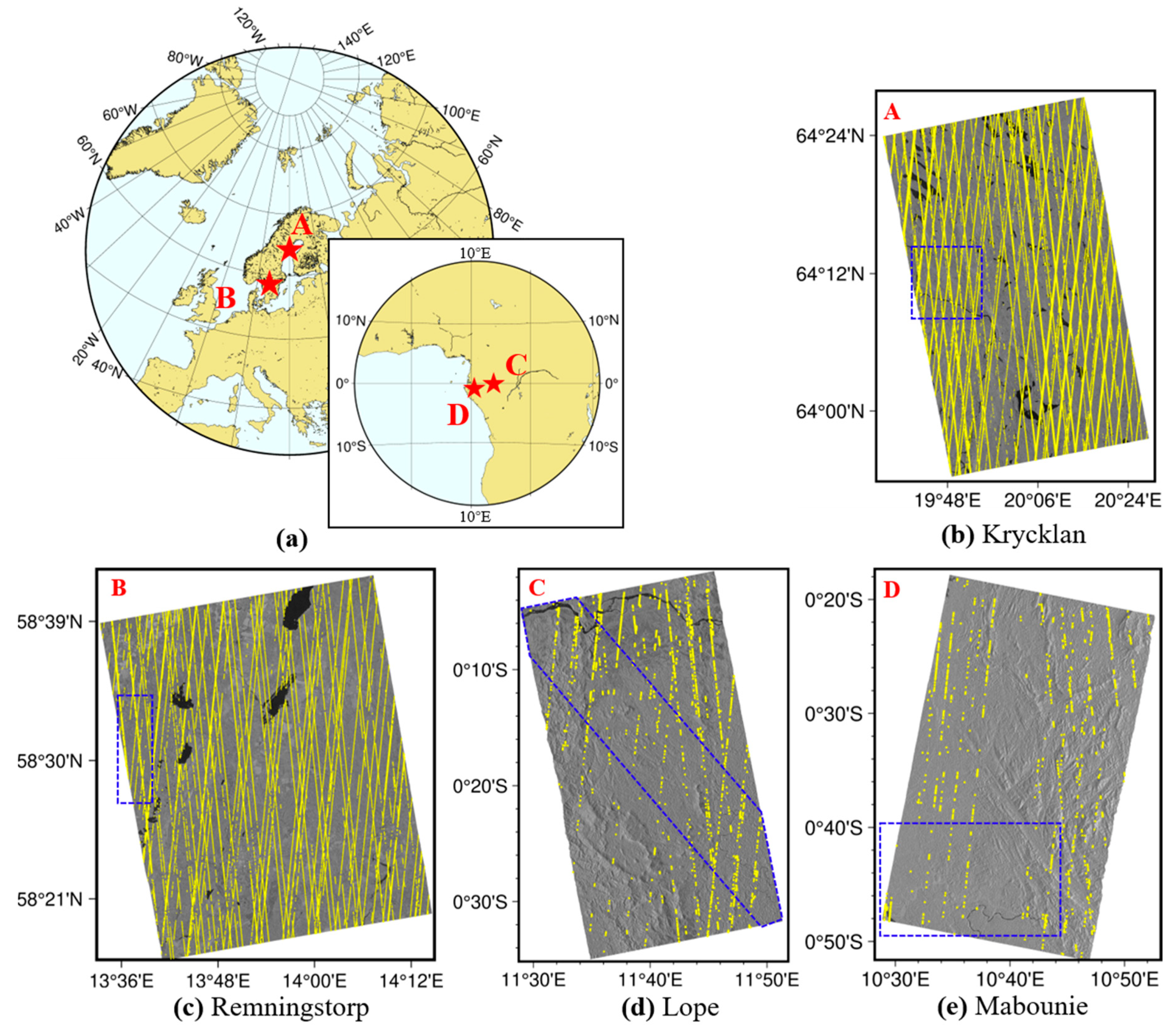
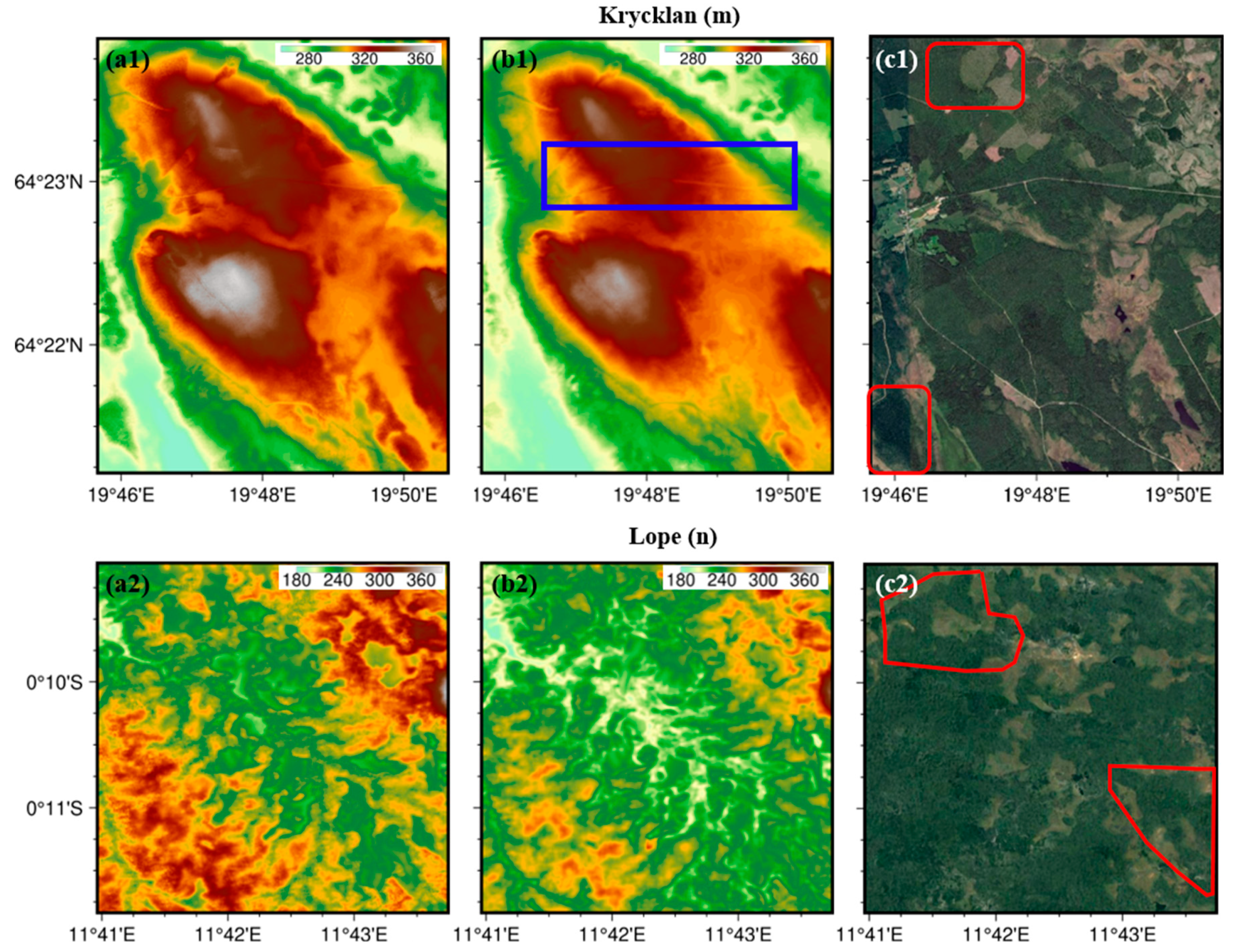
3.1. Study Area

Four test sites (A, B, C, D in Figure 4a) with different forest types and terrain were selected to test the applicability of the proposed method for estimating sub-canopy topography. The first test site (Figure 4b) is located in Krycklan in northern Sweden, where boreal coniferous forest dominates, with an average forest height of approximately 18 m. Hills are the main terrain at this test site, with several canyons and altitude ranges from 50 to 350 m. The second test site (Figure 4c) is located in Remningstorp, southern Sweden. The forest area is divided into a semi-northern area, with the tallest forest approximately 35 m. The terrain is relatively flat, except for the hills in the southwest, with elevations ranging from 120 m to 200 m. The third (Figure 4d) and fourth (Figure 4e) test sites are located in the Lope and Mabounie regions of Gabon, Africa. These two test sites are dominated by tall and dense tropical rainforests, with the tallest forest exceeding 60 m. The average forest height at the Lope test site is approximately 50 m, whereas that at the Mabounie test site is slightly lower, with an average height of approximately 30 m. These sites show visible topographic relief, and there are many fragmented slopes west of the Lope test site and northeast of the Mabounie test site, and the ground elevations range from 200 m to 750 m.

3.2. Datasets

3.2.1. TanDEM-X InSAR Data

Table 1. Geometric parameters of the TanDEM-X CoSSC data for the four test sites.

Test Site	Date	Incidence Angle (°)	Baseline (m)	HoA (m)	Polarization
Krycklan	28 July 2012	41.5°	185.9	−37.5	HH
Remningstorp	19 December 2011	41.5°	110.1	−65.9	HH
Lope	25 March 2014	45.9°	103.4	75.6	HH
Mabounie	5 November 2011	34.6°	114.3	50.5	HH

details the parameters of the TanDEM-X co-registered single-look slant-range complex (CoSSC) data used. All data were acquired with HH polarization between 2011 and 2015, and the interferometric baseline was between 103.4 m and 185.9 m. Although there are large baseline differences, their HoAs indicate that all data are suitable for measuring forest height in the corresponding test sites, with satisfactory sensitivity to forest height, density, and dielectric properties.

3.2.2. ICESat-2 ATL08 Data

The ICESat-2 satellite was launched in September 2018 and uses the Advanced Topographic Laser Altimetry System (ATLAS) to acquire global elevation information, whose measurements provide elevation data for a wide range of scientific disciplines [45,46]. In this study, we used the ATL08 product, which is the only along-track product that provides elevation data for land and vegetated surfaces [47], and all data were acquired from October 2018 to June 2022. To obtain reliable control points, it is necessary to screen the ATL08 data and retain as many points as possible while ensuring accuracy [48]. The yellow dots in Figure 4b–e show the tracks of the ICESat-2 control points after screening.

Table 2. The number and percentage of ICESat-2 data used for modeling.

Test Site	Number	Percentage
Krycklan	43,227	0.19%
Remningstorp	69,820	0.28%
Lope	5419	0.04%
Mabounie	3194	0.03%

shows the number of ICESat-2 control points used for modeling, ranging from several thousand to tens of thousands. Compared to the number of pixels in the entire test site, the data of the control points accounted for less than 0.3%.

3.2.3. Forest Non-Forest Map

The TanDEM-X Forest Non-forest (FNF) Map was obtained using DLR from TanDEM-X InSAR data [49], which included four categories: water, forest, non-forest, and urban areas. To avoid misestimating water and urban areas, we used the FNF map for masking.

3.2.4. Airborne LiDAR Data

As shown in Figure 4b–e, the blue dotted boxes show the coverage of high-precision and high-resolution airborne LiDAR data. The Swedish Defense Research Agency acquired high-precision LiDAR data from the Krycklan and Remningstorp test sites during the BIOSAR2007 and BIOSAR2008 missions [50,51], respectively. During the AfriSAR mission, NASA obtained high-precision LiDAR data from the Lope and Mabounie test sites [52]. The above LiDAR products were used to analyze and verify the accuracy of the estimated sub-canopy topography.

4. Results

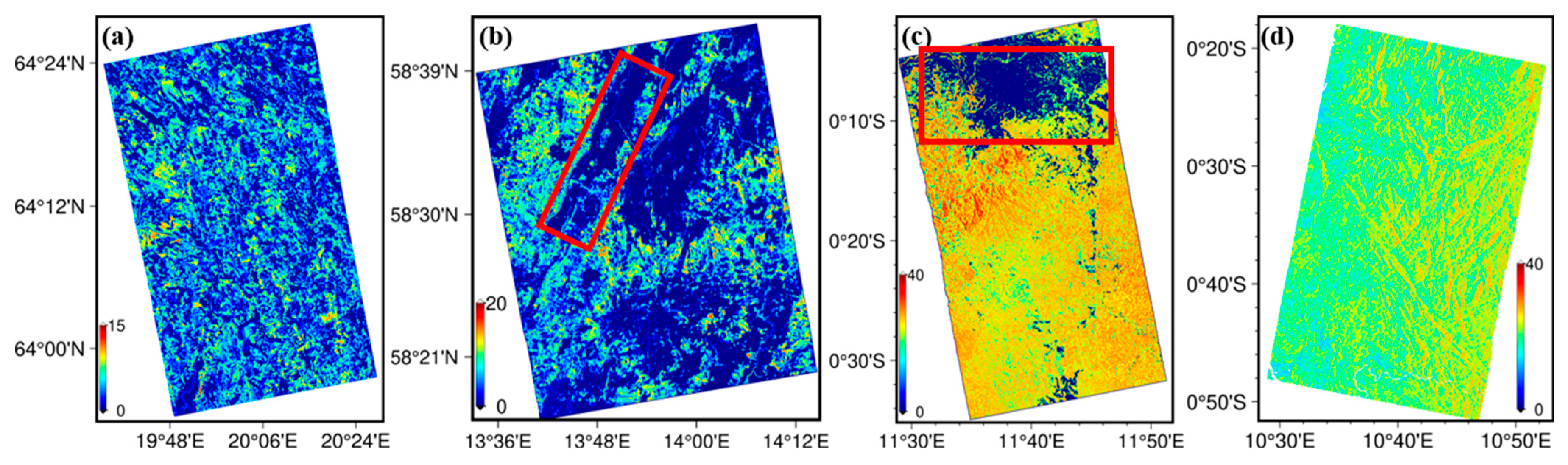
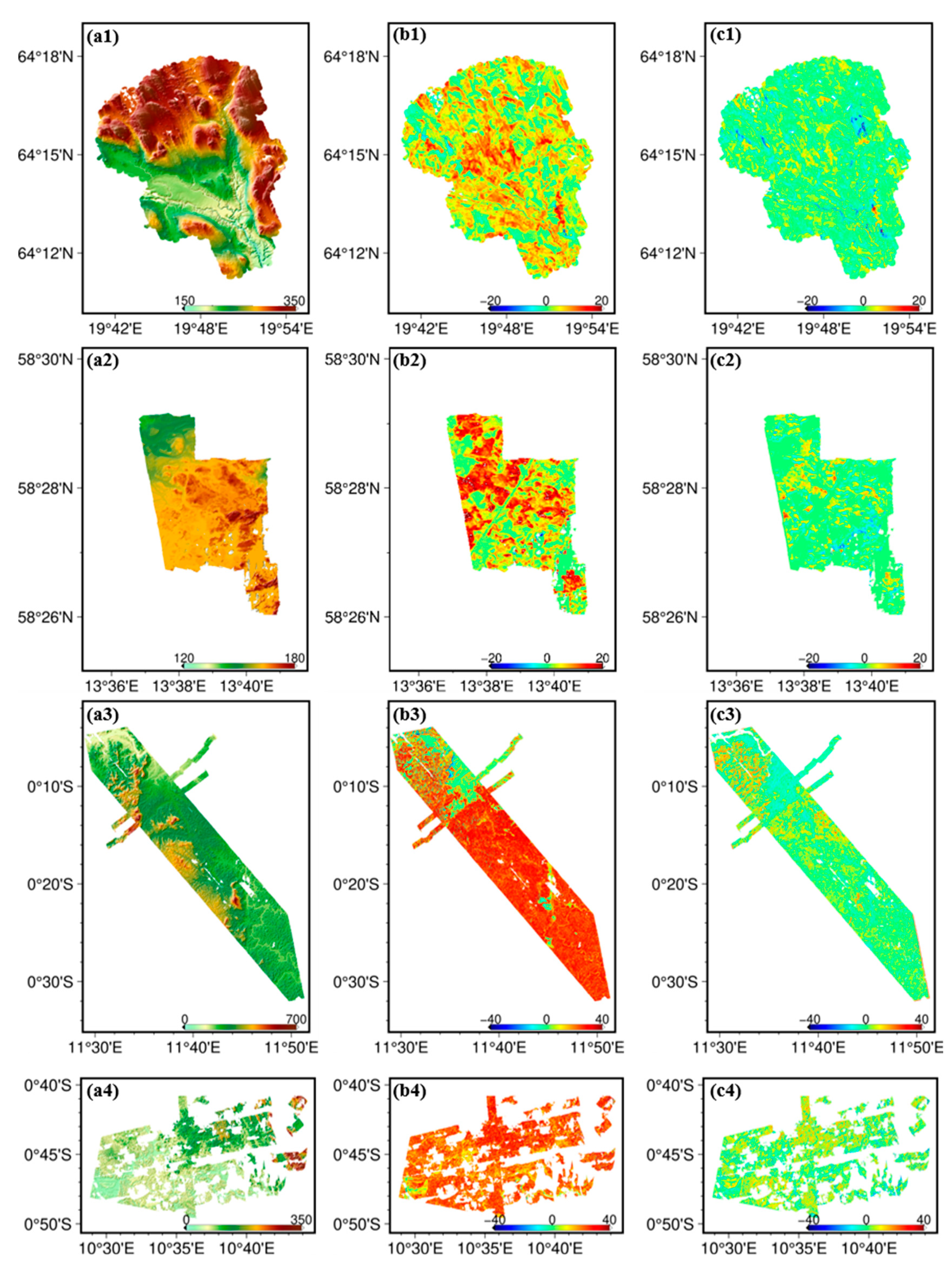
4.1. Comparison of InSAR-Derived DEM and LiDAR Data in Vegetated Areas

The original TanDEM-X CoSSC data were used to estimate DEM by interferometry. Low interferometric coherence (less than 0.3) and geometric distortion can cause severe data processing bias, so we mask these areas. Additionally, water and urban areas were masked using FNF maps.

As shown in

Table 3. Statistics of InSAR-derived DEM minus LiDAR products, classified by forest height in 10 m intervals.

Forest Height (m)	InSAR-Derived DEM—LiDAR DTM			Coherence	InSAR-Derived DEM—LiDAR DSM
	Mean (m)	STD (m)	Deviation Pixel Ratio (%)	Mean	Mean (m)	STD (m)	Deviation Pixel Ratio (%)
Krycklan
0~10	0.93	2.08	56.52	0.84	−5.54	2.60	96.25
10~20	5.05	3.28	91.76	0.82	−10.47	3.28	99.88
20~30	8.25	4.70	94.77	0.65	−13.99	4.59	99.98
Remningstorp
0~10	2.12	5.72	58.73	0.86	−2.82	6.01	84.97
10~20	6.69	5.32	92.50	0.81	−9.40	5.31	99.88
20~30	10.89	5.82	95.66	0.71	−12.66	5.60	99.98
>30	15.73	8.27	94.25	0.66	−15.37	8.19	100.00
Lope
0~10	0.79	8.72	80.96	0.84	−4.04	8.80	92.83
10~20	5.14	9.59	89.66	0.79	−9.55	9.53	96.45
20~30	11.89	7.89	97.21	0.75	−13.86	7.57	98.62
30~40	22.56	6.27	99.82	0.72	−13.93	5.74	99.33
40~50	29.64	6.47	99.98	0.68	−14.68	6.06	99.24
>50	36.67	8.48	99.99	0.73	−15.73	8.26	99.95
Mabounie
0~10	3.58	3.02	75.81	0.81	−1.73	4.29	88.90
10~20	5.76	2.74	94.78	0.72	−10.44	3.03	96.03
20~30	16.07	6.16	99.73	0.63	−10.42	5.98	98.01
30~40	22.64	6.63	99.93	0.51	−12.67	6.38	98.65
>40	28.32	8.44	99.90	0.46	−15.95	8.50	98.76

, the forest heights were grouped in intervals of 10 m, and the DEM was compared with the airborne LiDAR data. The performance of the TanDEM-X InSAR-derived DEM was analyzed by calculating SPC height and penetration depth. For the four test sites, the mean difference between the InSAR-derived DEM and LiDAR DTM increased significantly with vegetation height. For the mean, the average difference exceeded 30 m higher at forest heights ≥ 50 m than 0~10 m. In addition, compared to the LiDAR digital surface model (DSM), the InSAR signal exhibited penetrability, and the penetration depth increased with forest height. However, when forest height exceeded 20 m, the increasing trend of the penetration depth was significantly reduced. Considering the known limitations of X-band SAR signals in terms of forest penetration, this was not surprising.

Compared to the other three test sites, the rate of increase in the mean difference in DEM caused by forests was relatively small at the Krycklan test site. Owing to the sparse distribution and short forest at this test site, the influence of forests on the accuracy of the InSAR-derived DEM was weakened. In addition, we counted the number of pixels whose difference between InSAR-derived DEM and LiDAR DTM exceeded 0.5 m in each forest height interval, which increased with the increase in forest height. As shown in Table 3, the percentage of pixels with significant differences increased to approximately 100% in the group with the greatest vegetation height among the four test sites. A similar situation emerged when compared with the LiDAR DSM. In addition, the standard deviation between the InSAR-derived DEM and LiDAR data was relatively random, which was caused by forest type and density at different forest height intervals. Notably, interferometric coherence showed a significant correlation with the mean deviation, which decreased significantly with increased forest height. Based on this, interferometric coherence can become a key variable in the estimation of SPC height, highlighting its innovative contribution to this study.

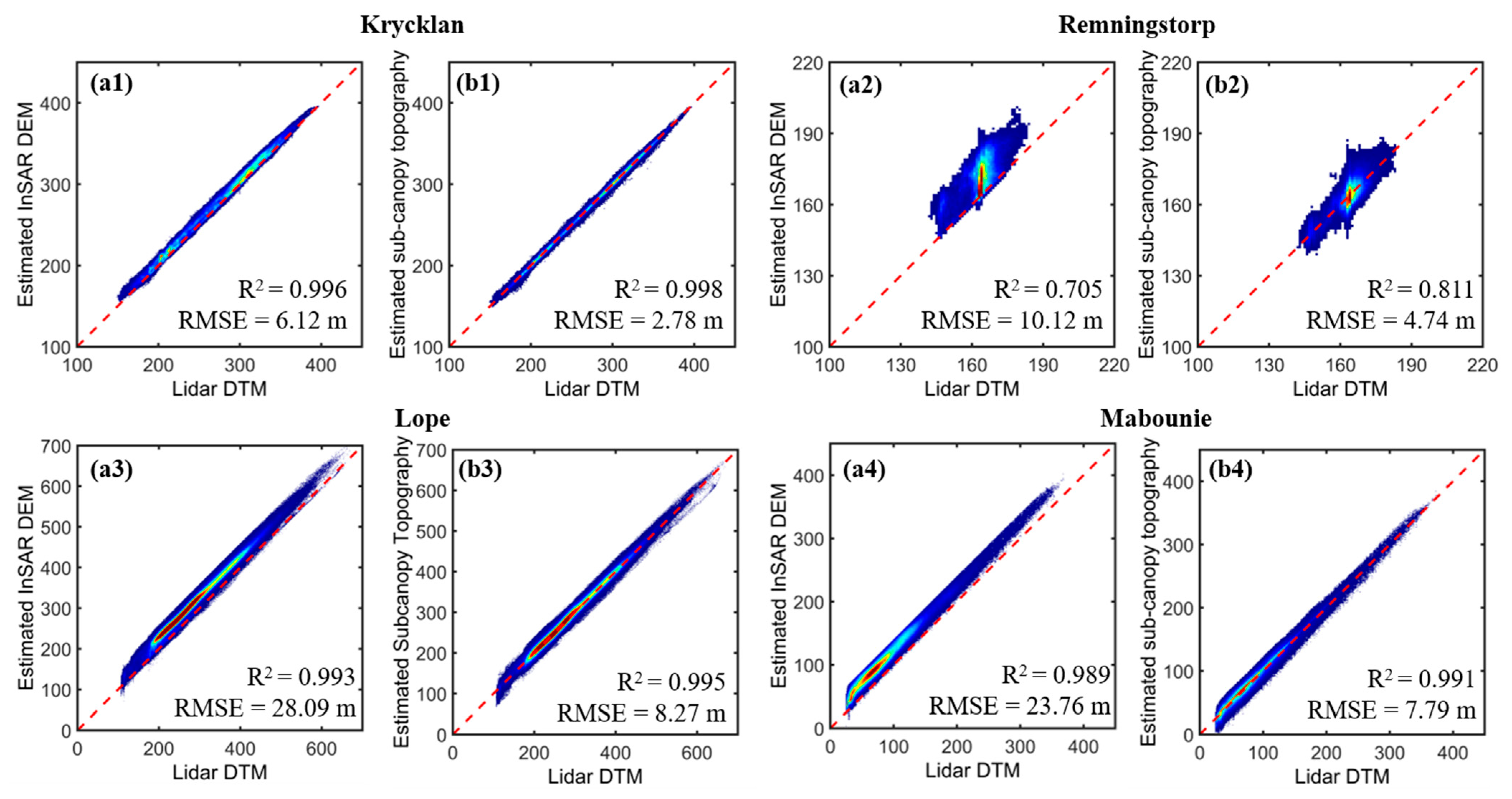
4.2. Validation of Estimated Sub-Canopy Topography with Airborne LiDAR DTM

Figure 5 shows the DEMs obtained from the TanDEM-X InSAR data for the four test sites. The topography of the Krycklan (Figure 5a) and Lope (Figure 5c) test sites was obviously undulating, whereas the topography of the remaining two test sites was relatively flat. Figure 6 shows the SPC height estimated using the proposed method. Because of the different forest heights and densities, the Krycklan test site (Figure 6a) was less affected by forest height, and the estimated average SPC height was approximately 5 m. The Lope test site (Figure 6c) was covered by dense tropical rainforests with an average forest height of approximately 50 m, and the estimated SPC height exceeded 30 m in most areas. These results are consistent with those presented in Table 3. In addition, the SPC height estimated by the proposed method also showed excellent performance for bare land and low-vegetation areas, especially at the Remningstorp and Lope test sites. As shown by the red rectangle in Figure 6b, the estimated SPC height of the farmland area was close to zero, and the boundary between farmland and forest was clearly apparent. In addition, the area shown by the red rectangle in Figure 6c is a grassland dominated by low shrubs. The estimated SPC height was significantly smaller than that of the rainforest area, and there is a very significant dividing line with the rainforest. This ability to discriminate demonstrated the robustness of the proposed method for different types of vegetation cover.

To demonstrate that the SPC was highly separated from the InSAR-derived DEM, local regions m and n, marked by blue rectangles in Figure 5, and profile AB, marked by the black solid line, were selected for analysis. Figure 7 enlarges the marked areas m and n, which assists in the intuitive analysis of the performance of the proposed method in separating SPC height signals, and also shows an optical image (Figure 7(c1,c2)) for comparison and reference. Compared to Figure 7(c1,c2), the vegetation-covered InSAR-derived DEM (Figure 7(a1,a2)) contains obvious forest signals, especially in the area marked with red solid lines, and the height gradient between bare ground and vegetation is clearly apparent. The elevation of the sub-canopy topography (Figure 7(b1,b2)) is significantly lower than that of the InSAR-derived DEM. In addition, the gradient between forest and non-forest boundaries appeared smoother, and terrain texture features were more prominent. Surprisingly, at the Krycklan test site, the road originally covered by trees became more visible, as shown by the blue rectangle in Figure 7(b1).

As shown in Figure 8, the estimated sub-canopy topography was further compared with the InSAR-derived DEM and LiDAR DTM by analyzing profile AB. For the four test sites, compared to the InSAR-derived DEM, the elevation of the sub-canopy topography was significantly reduced and was closer to the LiDAR DTM. Although there are deviations from the LiDAR DTM at some locations owing to model errors, the overall consistency demonstrates the feasibility of the proposed method for the estimation of sub-canopy topography.

To evaluate the acquired sub-canopy topography in detail, high-precision airborne LiDAR DTMs, represented by blue dashed boxes in Figure 4, were used for comparison. Figure 9(a1–a4) shows an overview of the InSAR-derived DEM of the four test sites, and Figure 9(b1–b4) shows the difference maps between the InSAR-derived DEM and the LiDAR DTM. Due to the influence of forest scattering, the InSAR-derived DEM was significantly higher than the LiDAR DTM. As shown in Figure 9(c1–c4), using the proposed method, the SPC height in the InSAR-derived DEM can be effectively removed, and the differences between sub-canopy topography and LiDAR DTM are mostly concentrated around zero. Furthermore, we used the LiDAR DTM to obtain statistics on the accuracy before and after SPC height correction in the vegetated area. As shown in Figure 10, the InSAR-derived DEMs were much higher than the ground truth values and contained significant vegetation signals. After removing SPC height signals, the coefficient of determination (R²) between sub-canopy topography and LiDAR DTM improved, particularly at the Remningstorp test site, from 0.705 to 0.811. Due to the different forest and terrain, the RMSE of InSAR-derived DEM ranged from 6.12 m to 28.09 m. For the sub-canopy topography, the RMSE of the forest area ranges from 2.78 m to 8.27 m, both of which were significant improvements. The improvement in accuracy of the four test sites after removing the SPC height was 54.5%, 53.1%, 70.5%, and 67.2%. The significantly improved RMSE further demonstrates the robustness of the proposed method for the estimation of sub-canopy topography for different terrains, forest types, and forest heights.

5. Discussion

5.1. Advantages of Using Coherence and Local Modeling

Many studies have attempted to predict forest height signals in an InSAR-derived DEM using regression analysis with a small number of optical variables and ICESat-2 elevation [20,22,25,26,27,28]. However, owing to the penetrability of InSAR signals, optical remote sensing cannot fully record forest properties measured by InSAR because it can only observe the forest surface and is limited by the availability of cloud-free data [29]. To verify the robustness of the proposed method for sub-canopy topography estimation, it was compared with the following two cases:

Case 1: Using Landsat Vegetation Continuous Field (VCF) data and slope for regression analysis to predict the SPC height [26]. Similar to the existing work, we selected the latest version of VCF in 2015 [53] and downloaded it from the USGS website (https://e4ftl01.cr.usgs.gov/MEASURES/GFCC30TC.003/2015.01.01/, accessed on 1 March 2023). The VCF data files used in this study are listed in

Table 4. Statistical results of the performance of three different methods for sub-canopy topography estimation. The percentage represents the accuracy improvement of sub-canopy topography estimated by different methods compared with InSAR DEM.

Test Site	InSAR-Derived DEM (RMSE)	Sub-Canopy Topography (RMSE)
		Case 1		Case 2		Proposed Method
Krycklan	6.12 m	3.49 m	43.1% ↑	3.41 m	44.2% ↑	2.78 m	54.5% ↑
Remningstorp	10.12 m	4.89 m	51.6% ↑	5.39 m	46.7% ↑	4.74 m	53.1% ↑
Lope	28.09 m	12.40 m	55.8% ↑	12.05 m	57.1% ↑	8.27 m	70.5% ↑
Mabounie	23.76 m	10.18 m	57.2% ↑	10.21 m	57.1% ↑	7.79 m	67.2% ↑
VCF data	p184r060, p184r061, p185r060, p185r061, p194r015, p195r019

.

Case 2: Replace the VCF data in Case 1 with the interferometric coherence obtained by TanDEM-X to verify the performance of the estimation of sub-canopy topography without relying on external forest information products. In contrast to the proposed method of fitting multiple models, both Cases 1 and 2 fit only one model.

Table 4 shows the RMSEs of the sub-canopy topography estimated by different methods compared with the LiDAR DTM, and shows the accuracy of the InSAR-derived DEM for reference. Compared with the InSAR-derived DEM, the accuracy of the sub-canopy topography obtained in Case 1 improved by more than 50% on average. When the VCF data were replaced with interferometric coherence (i.e., case 2), similar accuracies were observed, and the Krycklan and Lope test sites showed slightly better results. In summary, interferometric coherence can completely replace VCF data and is more suitable for estimations of SPC height in many cases. In addition, the proposed method using local modeling to estimate sub-canopy topography achieved better accuracy, with the accuracy of sub-canopy topography improved by nearly 60% on average, demonstrating the effectiveness and robustness of local modeling.

5.2. Correlation between Forest Height and the Accuracy of Sub-Canopy Topography

Figure 11 shows histograms of the RMSEs of InSAR-derived DEM and sub-canopy topography accuracy with forest height variation. The RMSE of the InSAR-derived DEM increased with forest height. In particular, at the Lope test site, when forest height exceeded 50 m, the RMSE reached 37.63 m. After removing SPC height, the accuracy of the sub-canopy topography significantly improved in each forest height range. However, the RMSE of sub-canopy topography remained larger in areas of tall forests than in areas of short forests. This is because the ICESat-2 system cannot detect the real surface in dense and tall forests [54,55]. For the Lope and Mabounie test sites, the RMSE of sub-canopy topography exhibited a trend of increase–decrease–increase, compared with the Krycklan and Remningstorp test sites, showing slightly worse accuracy in the forest height ranges of 0 m to 30 m. This was because there are few low-vegetation areas in the Lope and Mabounie test sites, and the SPC height in the low-vegetation area was significantly overestimated because of the influence of the adjacent area of high vegetation. This phenomenon of SPC height overestimation can be observed by comparing Figure 9(b3–b4) and Figure 9(c3–c4).

5.3. Limitations and Future Enhancements

In this study, we proposed a method for estimating sub-canopy topography using only TanDEM-X and ICESat-2 data. Validated at four test sites, the accuracy of the estimated sub-canopy topography product is satisfactory for most applications. However, the following limitations and future improvements must be further investigated to generalize the proposed method and achieve more accurate estimates of sub-canopy topography at large scales.

First, the core of the proposed method was to select ICESat-2 TCPs with the same or similar forest and slopes in the local area and use orthogonal polynomial modeling to predict SPC height. However, in forest areas with complex forest stands, there may also be differences in local forest conditions; therefore, it is necessary to develop more appropriate strategies for selecting ICESat-2 TCPs. In addition, the proposed method needs to model each pixel individually, which greatly increases the computational cost compared with traditional global modeling. Therefore, quickly and accurately selecting appropriate control points or using external remote sensing data for assisted modeling is key to accurately estimating sub-canopy topography.

Second, the advantage of using inverse distance weighting is that it considers the spatial heterogeneity of forest attributes, and can better characterize the local characteristics of spatial data. However, it is sensitive to gross errors. When ICESat-2 TCPs have large errors in a local region, the accuracy of estimated SPC height will be reduced. Therefore, it is necessary to extract more accurate ICESat-2 TCPs, such as a more suitable filtering method for extracting TCPs from the ICESat-2 raw data.

Finally, the proposed method requires sufficient ground control points to support modeling. In this study, the number of ICESat-2 TCPs in the Lope and Mabounie test sites was less than 0.1% of the corresponding TanDEM-X pixels, which led to an overestimation of SPC height in areas with low vegetation. In addition, comparing Figure 4 and Figure 9 of the Lope and Mabounie test sites, the error in estimating sub-canopy topography in the sparse area of the ICESat-2 TCPs was significantly larger than that in the dense area. To solve this problem, we must investigate whether it is necessary to introduce more spaceborne LiDAR data, including GEDI data. These results will help us further determine the relationship between InSAR observations and SPC height and achieve large-scale and higher-precision estimates of sub-canopy topography. These issues should be investigated in future studies.

6. Conclusions

There are a variety of methods to remove forest signals from InSAR-derived DEMs to estimate sub-canopy topography, such as regression analysis relying on external optical data. However, it is difficult to guarantee the consistency of temporal and spatial resolution of optical data and InSAR-derived DEM and the availability of cloud-free data. In contrast, the observations obtained by InSAR technology are not limited by the above problems, and fully record the forest characteristics measured from the InSAR perspective. Based on this, this study proposed a practical method for estimating sub-canopy topography by combining single-baseline, single-polarization TanDEM-X InSAR and ICESat-2 data. The proposed method has been tested in four test sites characterized by different vegetation and terrain. The results show that the SPC height caused by forests in InSAR-derived DEM is effectively eliminated. Afterward, we used high-precision LiDAR DTM for verification, the accuracy of sub-canopy topography in four test sites ranges from 2.78 m to 8.27 m. The successful results provide a basis for future work and explore the application of this method to the estimation of large-scale sub-canopy topography. In addition, given the effectiveness and robustness of the proposed method, it can be used as a supplementary tool for future spaceborne SAR missions to estimate sub-canopy topography, such as LT-1, TanDEM-L, and BIOMASS missions, when only single-baseline and single-polarization data are available.

References

1. De Paiva, R.C.D.; Buarque, D.C.; Collischonn, W.; Bonnet, M.-P.; Frappart, F.; Calmant, S.; Bulhoes Mendes, C.A. Large-Scale Hydrologic and Hydrodynamic Modeling of the Amazon River Basin. Water Resour. Res. 2013, 49, 1226–1243. [Google Scholar] [CrossRef]
2. Baade, J.; Schmullius, C. TanDEM-X IDEM Precision and Accuracy Assessment Based on a Large Assembly of Differential GNSS Measurements in Kruger National Park, South Africa. ISPRS J. Photogramm. Remote Sens. 2016, 119, 496–508. [Google Scholar] [CrossRef]
3. Ma, R.J. DEM Generation and Building Detection from Lidar Data. Photogramm. Eng. Remote Sens. 2005, 71, 847–854. [Google Scholar] [CrossRef]
4. Abrams, M.; Crippen, R.; Fujisada, H. ASTER Global Digital Elevation Model (GDEM) and ASTER Global Water Body Dataset (ASTWBD). Remote Sens. 2020, 12, 1156. [Google Scholar] [CrossRef]
5. Farr, T.G.; Rosen, P.A.; Caro, E.; Crippen, R.; Duren, R.; Hensley, S.; Kobrick, M.; Paller, M.; Rodriguez, E.; Roth, L.; et al. The Shuttle Radar Topography Mission. Rev. Geophys. 2007, 45, RG2004. [Google Scholar] [CrossRef]
6. Krieger, G.; Fiedler, H.; Zink, N.; Hajnsek, I.; Younis, M.; Huber, S.; Bachmann, M.; Gonzalez, J.H.; Werner, M.; Moreira, A. The TanDEM-X Mission: A Satellite Formation for High-Resolution SAR Interferometry. In Proceedings of the 2007 European Radar Conference, Munich, Germany, 10–12 October 2007; IEEE: New York, NY, USA, 2007; pp. 83–86. [Google Scholar]
7. Rizzoli, P.; Martone, M.; Gonzalez, C.; Wecklich, C.; Tridon, D.B.; Braeutigam, B.; Bachmann, M.; Schulze, D.; Fritz, T.; Huber, M.; et al. Generation and Performance Assessment of the Global TanDEM-X Digital Elevation Model. ISPRS J. Photogramm. Remote Sens. 2017, 132, 119–139. [Google Scholar] [CrossRef]
8. Rossi, C.; Gonzalez, F.R.; Fritz, T.; Yague-Martinez, N.; Eineder, M. TanDEM-X Calibrated Raw DEM Generation. ISPRS J. Photogramm. Remote Sens. 2012, 73, 12–20. [Google Scholar] [CrossRef]
9. Wang, H.; Fu, H.; Zhu, J.; Liu, Z.; Zhang, B.; Wang, C.; Li, Z.; Hu, J.; Yu, Y. Estimation of Subcanopy Topography Based on Single-Baseline TanDEM-X InSAR Data. J. Geod. 2021, 95, 84. [Google Scholar] [CrossRef]
10. Fu, H.; Zhu, J.; Wang, C.; Wang, H.; Zhao, R. Underlying Topography Estimation over Forest Areas Using High-Resolution P-Band Single-Baseline PolInSAR Data. Remote Sens. 2017, 9, 363. [Google Scholar] [CrossRef]
11. Fu, H.; Zhu, J.; Wang, C.; Li, Z. Underlying Topography Extraction over Forest Areas from Multi-Baseline PolInSAR Data. J. Geod. 2018, 92, 727–741. [Google Scholar] [CrossRef]
12. Liao, Z.; He, B.; Bai, X.; Quan, X. Improving Forest Height Retrieval by Reducing the Ambiguity of Volume-Only Coherence Using Multi-Baseline PolInSAR Data. IEEE Trans. Geosci. Remote Sens. 2019, 57, 8853–8866. [Google Scholar] [CrossRef]
13. Cloude, S.R.; Papathanassiou, K.P. Polarimetric SAR Interferometry. IEEE Trans. Geosci. Remote Sens. 1998, 36, 1551–1565. [Google Scholar] [CrossRef]
14. Papathanassiou, K.P.; Cloude, S.R. Single-Baseline Polarimetric SAR Interferometry. IEEE Trans. Geosci. Remote Sens. 2001, 39, 2352–2363. [Google Scholar] [CrossRef]
15. Fu, H.Q.; Zhu, J.J.; Wang, C.C.; Zhao, R.; Xie, Q.H. Underlying Topography Estimation over Forest Areas Using Single-Baseline InSAR Data. IEEE Trans. Geosci. Remote Sens. 2019, 57, 2876–2888. [Google Scholar] [CrossRef]
16. Peng, X.; Li, X.; Wang, C.; Zhu, J.; Liang, L.; Fu, H.; Du, Y.; Yang, Z.; Xie, Q. SPICE-Based SAR Tomography over Forest Areas Using a Small Number of P-Band Airborne F-SAR Images Characterized by Non-Uniformly Distributed Baselines. Remote Sens. 2019, 11, 975. [Google Scholar] [CrossRef]
17. Aghababaei, H.; Ferraioli, G.; Ferro-Famil, L.; Huang, Y.; D’Alessandro, M.M.; Pascazio, V.; Schirinzi, G.; Tebaldini, S. Forest SAR Tomography: Principles and Applications. IEEE Geosci. Remote Sens. Mag. 2020, 8, 30–45. [Google Scholar] [CrossRef]
18. Shiroma, G.H.X.; Lavalle, M. Digital Terrain, Surface, and Canopy Height Models From InSAR Backscatter-Height Histograms. IEEE Trans. Geosci. Remote Sens. 2020, 58, 3754–3777. [Google Scholar] [CrossRef]
19. Gallant, J.C.; Read, A.M.; Dowling, T.I. REMOVAL OF TREE OFFSETS FROM SRTM AND OTHER DIGITAL SURFACE MODELS. Int. Arch. Photogramm. Remote Sens. Spat. Inf. Sci. 2012, 39, 275–280. [Google Scholar] [CrossRef]
20. Su, Y.; Guo, Q. A Practical Method for SRTM DEM Correction over Vegetated Mountain Areas. ISPRS J. Photogramm. Remote Sens. 2014, 87, 216–228. [Google Scholar] [CrossRef]
21. Su, Y.; Guo, Q.; Ma, Q.; Li, W. SRTM DEM Correction in Vegetated Mountain Areas through the Integration of Spaceborne LiDAR, Airborne LiDAR, and Optical Imagery. Remote Sens. 2015, 7, 11202–11225. [Google Scholar] [CrossRef]
22. O’Loughlin, F.E.; Paiva, R.C.D.; Durand, M.; Alsdorf, D.E.; Bates, P.D. A Multi-Sensor Approach towards a Global Vegetation Corrected SRTM DEM Product. Remote Sens. Environ. 2016, 182, 49–59. [Google Scholar] [CrossRef]
23. Tan, P.; Zhu, J.; Fu, H.; Wang, C.; Liu, Z.; Zhang, C. Sub-Canopy Topography Estimation from TanDEM-X DEM by Fusing ALOS-2 PARSAR-2 InSAR Coherence and GEDI Data. Sensors 2020, 20, 7304. [Google Scholar] [CrossRef] [PubMed]
24. Hawker, L.; Uhe, P.; Paulo, L.; Sosa, J.; Savage, J.; Sampson, C.; Neal, J. A 30 m Global Map of Elevation with Forests and Buildings Removed. Environ. Res. Lett. 2022, 17, 024016. [Google Scholar] [CrossRef]
25. Zhogolev, A.; Savin, I. The Influence Correction of Boreal Forest Vegetation on SRTM Data. Geocarto Int. 2018, 33, 573–586. [Google Scholar] [CrossRef]
26. Magruder, L.; Neuenschwander, A.; Klotz, B. Digital Terrain Model Elevation Corrections Using Space-Based Imagery and ICESat-2 Laser Altimetry. Remote Sens. Environ. 2021, 264, 112621. [Google Scholar] [CrossRef]
27. Kulp, S.A.; Strauss, B.H. CoastalDEM: A Global Coastal Digital Elevation Model Improved from SRTM Using a Neural Network. Remote Sens. Environ. 2018, 206, 231–239. [Google Scholar] [CrossRef]
28. Enwright, N.M.; Kranenburg, C.J.; Patton, B.A.; Dalyander, P.S.; Brown, J.A.; Piazza, S.C.; Cheney, W.C. Developing Bare-Earth Digital Elevation Models from Structure-from-Motion Data on Barrier Islands. ISPRS J. Photogramm. Remote Sens. 2021, 180, 269–282. [Google Scholar] [CrossRef]
29. Rahman, M.M.; Csaplovics, E.; Koch, B. An Efficient Regression Strategy for Extracting Forest Biomass Information from Satellite Sensor Data. Int. J. Remote Sens. 2005, 26, 1511–1519. [Google Scholar] [CrossRef]
30. Martone, M.; Braeutigam, B.; Rizzoli, P.; Gonzalez, C.; Bachmann, M.; Krieger, G. Coherence Evaluation of TanDEM-X Interferometric Data. ISPRS J. Photogramm. Remote Sens. 2012, 73, 21–29. [Google Scholar] [CrossRef]
31. Lopez-Sanchez, J.M.; Vicente-Guijalba, F.; Erten, E.; Campos-Taberner, M.; Javier Garcia-Haro, F. Retrieval of Vegetation Height in Rice Fields Using Polarimetric SAR Interferometry with TanDEM-X Data. Remote Sens. Environ. 2017, 192, 30–44. [Google Scholar] [CrossRef]
32. Martone, M.; Brautigam, B.; Krieger, G. Quantization Effects in TanDEM-X Data. IEEE Trans. Geosci. Remote Sens. 2015, 53, 583–597. [Google Scholar] [CrossRef]
33. Rizzoli, P.; Dell’Amore, L.; Bueso-Bello, J.-L.; Gollin, N.; Carcereri, D.; Martone, M. On the Derivation of Volume Decorrelation from TanDEM-X Bistatic Coherence. IEEE J. Sel. Top. Appl. Earth Obs. Remote Sens. 2022, 15, 3504–3518. [Google Scholar] [CrossRef]
34. Balss, U.; Breit, H.; Duque, S. TanDEM-X Payload Ground Segment: CoSSC Generation and Interferometric Considerations. Ger. Aerosp. Cent. 2012. Available online: https://tandemx-science.dlr.de/ (accessed on 1 December 2023).
35. Rabus, B.; Eineder, M.; Roth, A.; Bamler, R. The Shuttle Radar Topography Mission—A New Class of Digital Elevation Models Acquired by Spaceborne Radar. ISPRS J. Photogramm. Remote Sens. 2003, 57, 241–262. [Google Scholar] [CrossRef]
36. Al-Nuaimi, M.O.; Hammoudeh, A.M. Measurements and Predictions of Attenuation and Scatter of Microwave Signals by Trees. IEE Proc. Microw. Antennas Propag. 1994, 141, 70–76. [Google Scholar] [CrossRef]
37. Wang, F.; Sarabandi, K. A Physics-Based Statistical Model for Wave Propagation through Foliage. IEEE Trans. Antennas Propag. 2007, 55, 958–968. [Google Scholar] [CrossRef]
38. Caicoya, A.T.; Kugler, F.; Hajnsek, I.; Papathanassiou, K.P. Large-Scale Biomass Classification in Boreal Forests with TanDEM-X Data. IEEE Trans. Geosci. Remote Sens. 2016, 54, 5935–5951. [Google Scholar] [CrossRef]
39. Persson, H.J.; Olsson, H.; Soja, M.J.; Ulander, L.M.H.; Fransson, J.E.S. Experiences from Large-Scale Forest Mapping of Sweden Using TanDEM-X Data. Remote Sens. 2017, 9, 1253. [Google Scholar] [CrossRef]
40. Cloude, S.R. Polarisation: Applications in Remote Sensing; Oxford University Press: London, UK, 2009. [Google Scholar]
41. Denbina, M.; Simard, M. The Effects of Temporal Decorrelation and Topographic Slope on Forest Height Retrieval Using Airborne Repeat-Pass L-Band Polarimetric SAR Interferometry. In Proceedings of the 2016 IEEE International Geoscience and Remote Sensing Symposium (IGARSS), Beijing, China, 10–15 July 2016; pp. 1745–1748. [Google Scholar]
42. Nievergelt, Y. A Tutorial History of Least Squares with Applications to Astronomy and Geodesy. J. Comput. Appl. Math. 2000, 121, 37–72. [Google Scholar] [CrossRef]
43. Lee, J. A Reformulation of Weighted Least Squares Estimators. Am. Stat. 2009, 63, 49–55. [Google Scholar] [CrossRef]
44. Lu, G.Y.; Wong, D.W. An Adaptive Inverse-Distance Weighting Spatial Interpolation Technique. Comput. Geosci. 2008, 34, 1044–1055. [Google Scholar] [CrossRef]
45. Markus, T.; Neumann, T.; Martino, A.; Abdalati, W.; Brunt, K.; Csatho, B.; Farrell, S.; Fricker, H.; Gardner, A.; Harding, D.; et al. The Ice, Cloud, and Land Elevation Satellite-2 (ICESat-2): Science Requirements, Concept, and Implementation. Remote Sens. Environ. 2017, 190, 260–273. [Google Scholar] [CrossRef]
46. Magruder, L.; Neumann, T.; Kurtz, N. ICESat-2 Early Mission Synopsis and Observatory Performance. Earth Space Sci. 2021, 8, e2020EA001555. [Google Scholar] [CrossRef] [PubMed]
47. Neuenschwander, A.; Pitts, K. The ATL08 Land and Vegetation Product for the ICESat-2 Mission. Remote Sens. Environ. 2019, 221, 247–259. [Google Scholar] [CrossRef]
48. Li, Y.; Fu, H.; Zhu, J.; Wang, C. A Filtering Method for ICESat-2 Photon Point Cloud Data Based on Relative Neighboring Relationship and Local Weighted Distance Statistics. IEEE Geosci. Remote Sens. Lett. 2021, 18, 1891–1895. [Google Scholar] [CrossRef]
49. Martone, M.; Rizzoli, P.; Wecklich, C.; Gonzalez, C.; Bueso-Bello, J.-L.; Valdo, P.; Schulze, D.; Zink, M.; Krieger, G.; Moreira, A. The Global Forest/Non-Forest Map from TanDEM-X Interferometric SAR Data. Remote Sens. Environ. 2018, 205, 352–373. [Google Scholar] [CrossRef]
50. Hajnsek, I.; Scheiber, R.; Lee, S.; Ulander, L.; Gustavsson, A.; Tebaldini, S.; Monte Guarnieri, A. BIOSAR 2007: Technical Assistance for the Development of Airborne SAR and Geophysical Measurements during the BioSAR 2007 Experiment. Available online: https://elib.dlr.de/5992/ (accessed on 3 February 2023).
51. Hajnsek, I.; Keller, M.; Lee, S.; Horn, R.; Scheiber, R.; Papathanassiou, K.; Gustavsson, A.; Ulander, L.; Sandberg, G.; Le Toan, T.; et al. Biosar 2008: Data Acquisition and Processing Report. Available online: https://elib.dlr.de/63148/ (accessed on 1 December 2023).
52. Fatoyinbo, T.; Armston, J.; Simard, M.; Saatchi, S.; Denbina, M.; Lavalle, M.; Hofton, M.; Tang, H.; Marselis, S.; Pinto, N.; et al. The NASA AfriSAR Campaign: Airborne SAR and Lidar Measurements of Tropical Forest Structure and Biomass in Support of Current and Future Space Missions. Remote Sens. Environ. 2021, 264, 112533. [Google Scholar] [CrossRef]
53. Sexton, J.O.; Song, X.-P.; Feng, M.; Noojipady, P.; Anand, A.; Huang, C.; Kim, D.-H.; Collins, K.M.; Channan, S.; DiMiceli, C.; et al. Global, 30-m Resolution Continuous Fields of Tree Cover: Landsat-Based Rescaling of MODIS Vegetation Continuous Fields with Lidar-Based Estimates of Error. Int. J. Digit. Earth 2013, 6, 427–448. [Google Scholar] [CrossRef]
54. Liu, A.; Cheng, X.; Chen, Z. Performance Evaluation of GEDI and ICESat-2 Laser Altimeter Data for Terrain and Canopy Height Retrievals. Remote Sens. Environ. 2021, 264, 112571. [Google Scholar] [CrossRef]
55. Urbazaev, M.; Hess, L.L.; Hancock, S.; Sato, L.Y.; Ometto, J.P.; Thiel, C.; Dubois, C.; Heckel, K.; Urban, M.; Adam, M.; et al. Assessment of Terrain Elevation Estimates from ICESat-2 and GEDI Spaceborne LiDAR Missions across Different Land Cover and Forest Types. Sci. Remote Sens. 2022, 6, 100067. [Google Scholar] [CrossRef]
Figure 1. A schematic of the workflow for estimation of sub-canopy topography.
Remotesensing 16 01155 g001
Figure 2. Effects of vegetation and different surface slopes on TanDEM-X InSAR signal acquisition DEM. (a) Flat surface, (b) The surface aspect toward the TanDEM-X satellite, (c) The surface aspect opposite to the TanDEM-X satellite.
Remotesensing 16 01155 g002
Figure 4. Study area and data used. The red five-pointed stars in (a) indicate the geographic locations of the study areas. In the following four illustrations (be), the base map is the InSAR backscatter intensity map, the blue dotted box indicates coverage of airborne LiDAR verification data, and the yellow dots are ICESat-2 control points.
Remotesensing 16 01155 g004
Figure 5. DEMs estimated from TanDEM-X InSAR data: (ad) are the DEMs of the Krycklan, Remningstorp, Lope and Mabounie test sites respectively. The blue rectangle represents the area used for enlarged analysis in Figure 7, and the black solid line AB represents the location of the profiles in Figure 8.
Remotesensing 16 01155 g005
Figure 6. The SPC heights estimated by the proposed method: (ad) are the SPC heights of the Krycklan, Remningstorp, Lope and Mabounie test sites respectively. The red rectangular highlight results for forested and non-forested areas.
Remotesensing 16 01155 g006
Figure 7. Enlarged view of regions m and n marked with blue rectangular boxes in Figure 5. (a1,a2) InSAR-derived DEM, (b1,b2) sub-canopy topography, (c1,c2) true color image acquired by the Landsat 8 satellite. The red line box is used to analyze areas where the SPC height is significantly removed from the DEM.
Remotesensing 16 01155 g007
Figure 8. Elevation profiles at the location of line AB marked in Figure 5: (ad) correspond to the profiles marked at the Krycklan, Remningstorp, Lope, and Mabounie test sites in Figure 5, respectively.
Remotesensing 16 01155 g008
Figure 9. DEM comparison with airborne LiDAR DTM before and after removing SPC height. (a1a4) Airborne LiDAR DTM. (b1b4) InSAR-derived DEM minus LiDAR DTM. (c1c4) Sub-canopy topography minus LiDAR DTM. Top to bottom are Krycklan, Remningstorp, Lope, and Mabounie test sites, respectively.
Remotesensing 16 01155 g009
Figure 10. Scatterplots to verify the accuracy of the InSAR-derived DEM and sub-canopy topography using the airborne LiDAR DTM, with colors representing scatterplots density increasing from blue to red. (a1a4) The accuracy of InSAR-derived DEM, (b1b4) the accuracy of sub-canopy topography.
Remotesensing 16 01155 g010
Figure 11. RMSE statistical histogram of InSAR-derived DEM and sub-canopy topography at different forest height intervals. (a1a4) The accuracy of InSAR-derived DEM; (b1b4) the accuracy of sub-canopy topography.
Remotesensing 16 01155 g011