Abstract
Natural hazards are considered to have a strong link with climate change and human activities. With the rapid advancements in remote sensing technology, real-time monitoring and high-resolution remote-sensing images have become increasingly available, which provide precise details about the Earth’s surface and enable prompt updates to support risk identification and management. This paper proposes a new network framework with Transformer architecture and a Residual network for detecting the changes in high-resolution remote-sensing images. The proposed model is trained using remote-sensing images from Shandong and Anhui Provinces of China in 2021 and 2022 while one district in 2023 is used to test the prediction accuracy. The performance of the proposed model is evaluated by using five matrices and further compared to both convention-based and attention-based models. The results demonstrated that the proposed structure integrates the great capability of conventional neural networks for image feature extraction with the ability to obtain global context from the attention mechanism, resulting in significant improvements in balancing positive sample identification while avoiding false positives in complex image change detection. Additionally, a toolkit supporting image preprocessing is developed for practical applications.
1. Introduction
The occurrence and severity of natural disasters, such as floods, droughts, sea level rise, landslides, heat or cold waves, etc., are considered to have a strong link with climate change and human activities [1,2,3]. Climate change tends to alter the characteristics of these hazards, while human infrastructure can amplify or reduce the potential risk of them [2,4,5]. For example, due to rapid urbanization and economic development, human activities such as excavation, occupation, building, and road construction can increase flood risk by altering the flow routine during rainfall events [6]. Therefore, enhancing supervision is one of the most effective approaches to reducing anthropogenic influence by promptly identifying and monitoring these behaviors [7]. With the rapid advancement in remote sensing technology, real-time monitoring over the targeted regions can be achieved without manual inspection efforts. In particular, high-resolution remote-sensing images have become gradually available, which can provide precise details about Earth’s surface conditions at a fine scale and allow for rapid updates in observations to support risk assessment of natural hazards [8,9]. By using the monitoring images, the changes of human infrastructure can then be detected, where the risky behaviors can be identified. However, how to deal with remote-sensing images with high resolution accurately and effectively is still challenging. One of the most significant problems is that although high resolution enhances finer spatial details for object recognition, the sensitivity to illumination conditions and occasional interruptions also increases during the procedure of image collection. Additionally, the remote-sensing images usually tend to be large-sized and require segmentation, resulting in inconsistency, particularly at the boundaries.
To identify the changes of the objects based on images, several methods have been proposed and widely applied to various fields related to engineering and environment monitoring for several decades such as image differencing [10], principal component analysis [11], image fusion [12], thresholding techniques [13], and object-based detection [14]. The typical steps of these methods usually involve an initial preprocessing of input images by carrying out normalization to mitigate the impact of variations in illumination and colors. Then, pixel-based calculations and transformations are performed using approaches such as the histogram of oriented gradients [15] and the scale-invariant feature transform [16]. Finally, image features are extracted while changes can be detected by calculating the differences between pixels. However, simple normalization is insufficient to effectively mitigate disturbances such as illumination and sensor noises during collection. These basic steps fail to extract the deep semantic features embedded within the images by disregarding the contextual information as they focus more on detecting the pixel or regional-level changes or differences [17]. Moreover, the values of the parameters governing the change detection within these methods are usually defined manually, which greatly relies on the expertise of modelers and the entire process can be time-consuming.
With the great improvement in calculation computation capacity, new technologies such as deep learning have demonstrated their potential in pattern recognition and feature extraction [18,19,20]. Different from the conventional methods, deep learning models can achieve a higher detection accuracy via automatic training by using sufficient labeled data; the features of the images can then be identified and extracted. There are many deep learning methods for extracting spatial information features of images. Most recent studies employ convolutional neural networks (CNNs) to deal with large datasets for feature extraction [21,22,23,24], which are also very popular in the field of remote-sensing image change detection such as dual attentive fully convolutional Siamese networks (DASNets) [25], triplet-based semantic relation networks [26], deep feature difference convolutional neural networks [27], dual-task constrained deep Siamese convolutional networks [28], deeply supervised image fusion networks [29], and many networks based on the U-Net structure [30,31,32], to name a few. Additionally, to optimize the spatial information within the images, several deep frameworks are developed to reduce the information loss [33,34], which can be combined with CNNs for classification and pattern recognition. However, as a CNN is primarily designed for extracting the local features, when dealing with large-sized images, it shows limitations in perceiving global information such as long-range spatial and temporal relationships among features in the context.
To obtain the contextual information, some attention-based approaches have been proposed in the past several years such as channel attention [28,29,35,36,37], spatial attention [28,29,35] and self-attention [25,36,38]. By incorporating them, the performance of the network structure based on bitemporal features becomes generally better than the effect of channel-wise concatenation [38,39,40]. In particular, the Vision Transformer (ViT) [41,42], as a new self-attention structure for computer vision, has gained remarkable achievements in language processing and other AI-related fields. The basic idea of this structure is to follow the multi-head attention with a feed forward network (FFN) where the global contextual information can be obtained by the multi-head attention and interact channel-wise.
Since the high-resolution remote-sensing images contain numerous geographical details of the monitoring objects, which are usually spatiotemporal, nonstationary, large-sized, intricate with high dimensions [43], it greatly challenges pattern recognition by using conventional CNNs. Not only the local features of images but also their global interaction in the context is essential for improving the performance of pattern recognition and change detection. To contribute to this knowledge, in this paper, we propose a new, hybrid CNN-ViT framework named ResNet18+Transformer for detecting changes from high-resolution remote-sensing images. This model framework incorporates the Vision Transformer into a CNN and renovates the layer structure to leverage the advantages of ViT in capturing global features and CNN’s expertise in local features. The data collected for model training are remote-sensing image samples from Shandong Province and Anhui Province of China with a resolution of 2 m. The training samples are divided into two phases: images captured at the same location in the years of 2021 and 2022, where manual marks are made to identify the changes in buildings, river channels or pipelines, newly constructed roads, and large-scale alterations resulting from human activities such as excavation, occupation, dumping, or surface damage. The trained model is further applied to detect the changes in Yaohai District by using the remote-sensing image of 2023, where the accuracy and efficiency are evaluated. Additionally, to support the remote-sensing images and result processing and increase the practical applications, we also design a toolkit for automatic image processing including image cropping, result splicing, and vector conversion.
The remainder of this paper is organized as follows: Section 2 describes the development of the framework of the hybrid CNN-ViT model proposed for building change detection while the details of the case are explained; Section 3 describes the demonstration case for detecting changes in two provinces of China by applying the proposed mode; Section 4 discusses the performance and flexibility of the proposed mode. Finally, the conclusion is given in Section 5.
2. Methodology
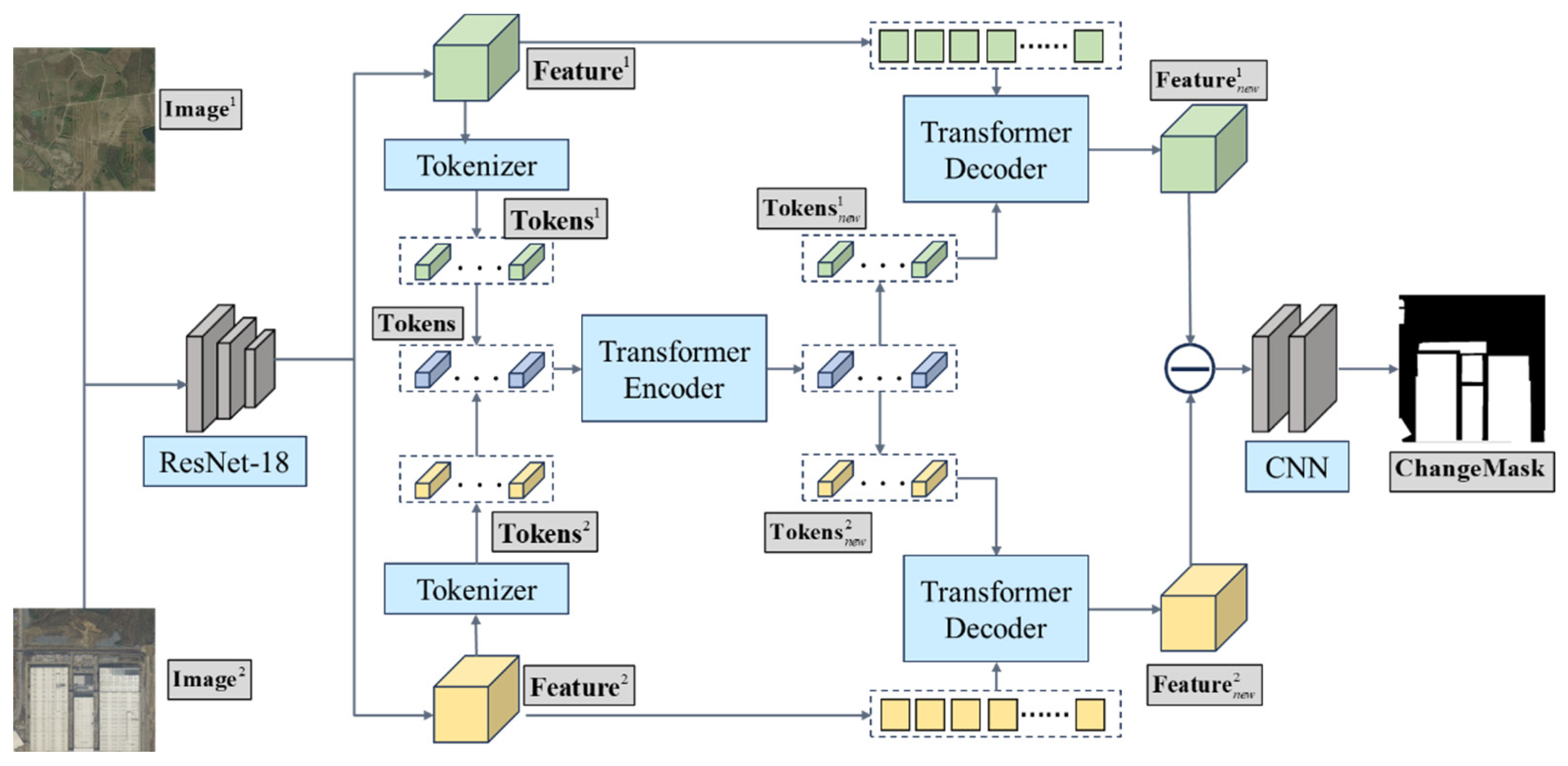
Figure 1 presents the framework of the hybrid CNN-ViT model deep learning model developed for detecting changes from the remote-sensing images filled with complex details by capturing the differences between the two phases of images. The overall architecture illustrated in Algorithm 1 consists of three main components of the framework, i.e., initial feature extraction, Transformer-based network development, and Prediction Head construction, which are elaborated in the following subsections.
| Algorithm 1. The overall architecture of the ResNet18+Transformer deep learning model for change detection |
| 1: Input::: 2: Load pretrained ResNet-18 network and feature extraction 3: 4: 5: function Tokenizer() 6: 7: 8: 9: end function 10: function TransformerEncoder(Tokens) 11: Initialize Transformer encoder layers 12: 13: 14: 15: end function 16: function TransformerDecoder() 17: Initialize Transformer decoder layers 18: 19: 20: 21: 22: end function 23: function PredictionHead() 24: Initialize decoding layers 25: 26: 27: 28: 29: end function |
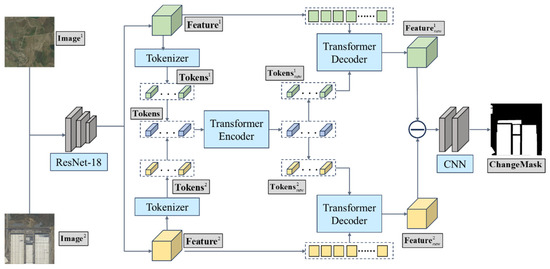
Figure 1.
The framework of the ResNet18+Transformer deep learning model for change detection.
The first step of the modelling framework is to extract the features from two images to be compared, using a pre-trained ResNet-18 network (more details can be found at https://download.pytorch.org/models, (accessed on 23 March 2024)). By implementing this, the two images ( and ) are transformed into certain corresponding feature tensors, e.g., and with the size of (height × width × number of channels) where the superscript number indicates different images. These feature tensors contain the substantial, basic visual information of the images, which serves as the input of the transformer-based network.
The second step is to construct the new, transformer-based network for extracting deep features from these tensors. ( and ) by taking the context into account. This step incorporates the self-attention mechanism to carry out context-aware feature transformation and employed a semantic Tokenizer to downsample the image features. It generates the sequences and with the size of . Then the sequences from the two images are merged into one single sequence with the length of . The merged sequence is fed to a Transformer Encoder, where the multiple-layer self-attention mechanism and feedforward neural networks are applied to generate a new sequence Tokensnew where the context information is fully involved. Then the new sequence is split back into two, i.e., and of and , which are mapped to the decoded, context-aware image features and by using a transformer decoder.
The last step is to build the Prediction Head for converting the context-aware features and to the change mask which can be used to represent the changing area in the images. It can be achieved by subtracting the two decoded image features, where their absolute difference is taken to generate the feature map. This map is then input to a fully convolutional network consisting of two convolutional layers and batch normalization and a pixel-level change mask are generated and highlighted back to the images, where the change area is detected.
2.1. Initial Feature Extraction
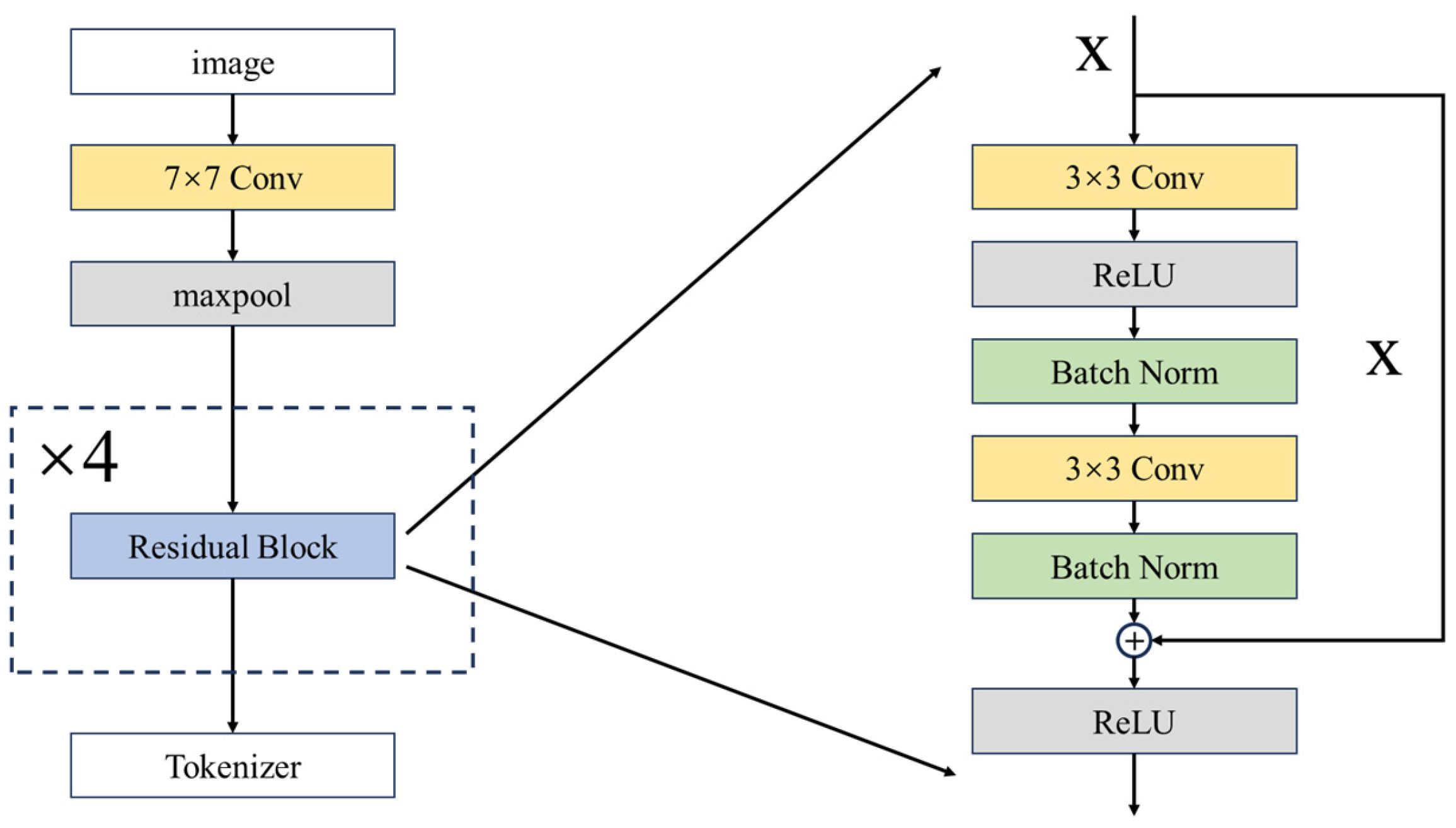
During the first step of image feature extraction, we incorporate a residual network ResNet-18 into our framework to mitigate the issues of gradient vanishing and degradation commonly found in deep learning models [44]. The inclusion of the ResNet-18 aims to enhance the model capacity for complex task training and performance maintenance, given that remote-sensing images usually encompass abundant information with high dimensions. The fundamental architecture of ResNet-18 usually comprises convolutional layers, residual blocks, and fully connected layers; however, the fully connected layers are excluded in our framework where the result from the residual blocks is directly fed to the tokenizer. The developed structure of ResNet-18 is presented in Figure 2.

Figure 2.
ResNet-18 architecture developed for the model framework.
The core of the ResNet-18 is the four residual blocks where each involves convolution operation, batch normalization, and activation. The input of the residual block are the feature tensors that are initially extracted from a simple convolution; the first convolution layer of the residual block transformed using an kernel and stride (see Equation (1)) and applies the ReLU (Rectified Linear Unit) on it.
where denotes the parameters of the current convolutional kernel and indicates the convolution operation which was used for the initial feature extraction.
Then batch normalization is followed to facilitate the convergence of training and enhance the model stability, which can be written as:
where indicates the output feature tensor of the upper the convolution layer, and denote the mean and standard deviation of the features, and and denote the scale and shift parameters of batch normalization, respectively.
Similar to the abovementioned, a convolutional layer with a kernel followed by batch normalization is applied in a repeated manner (see Figure 2). The output of these is added to then applied to the ReLU, which is called skip connection. This connection enables the direct transmission of the information (i.e., the feature tensors) to mitigate the risk of information loss during deep network training; the equation can be written as:
where represents the output of the multiple convolution operation and batch normalization.
2.2. Transformer-Based Network
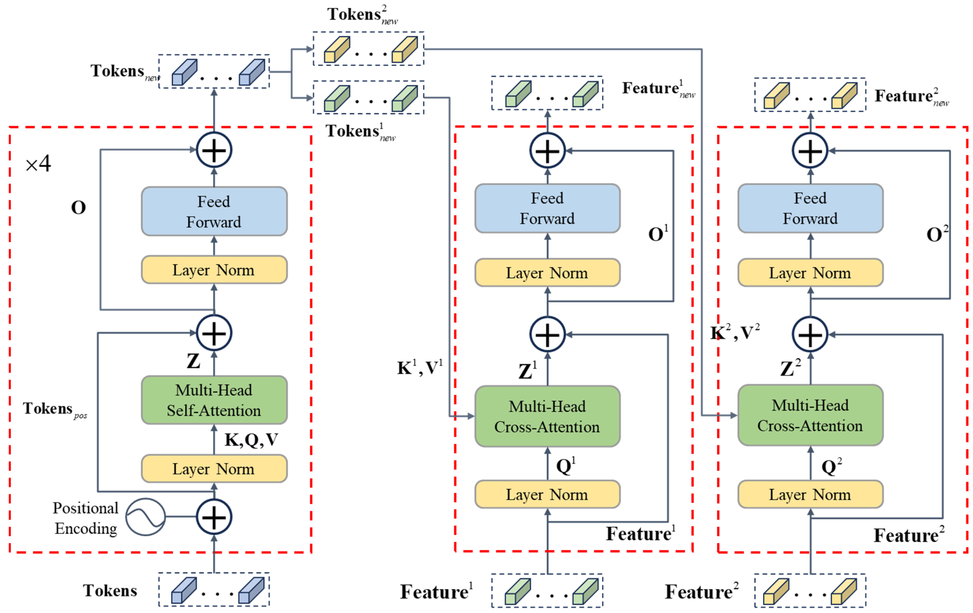
Figure 3 presents the architecture of the Transformer-based network we developed; the details of each module are presented below.
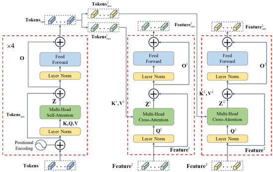
Figure 3.
The structure of the transformer-based network.
2.2.1. Tokenizer
After applying ResNet-18, we extract semantic information from the feature tensors by developing a Tokenizer and the tensor is transformed into Tokens where indicates the th image. The is the output of ResNet-18 with the size of , where and indicate the height and width of the feature map and is the channel dimension of the feature. A convolution operation for the pixel is applied to using a kernel , resulting in a feature denoted as . is normalized through a softmax function and an attention map is generated, with all the elements summing up to 1.0. Then the map is element-wise multiplied by the down-sampled feature , and the calculation result is unfolded into a line sequence called Tokens (see Equation (4)). It should be noted that Tokens incorporate positional weights that represent distinct semantic regions within the image. The two Tokens and from both images are merged into one sequence Tokens as the input of the Transformer Encoder.
2.2.2. Transformer Encoder
In order to capture the contextual information of the image and integrate it into feature tokens, the self-attention mechanism is employed in the developed Transformer Encoder which includes 4 layers and runs 4 times to generate the new, context-aware sequence .
Since the positioning of the elements in the sequence was significant, we first incorporate a positional encoding method to , which is set to be trained concurrently with the entire network. Then the positional encoding of each element is subsequently appended to the sequence , resulting in Tokens encompassing position information which is also the residual to be added to the third layer.
Different from the conventional Transformer, we set up the first layer of the encoder as layer normalization to enhance the stability of the network (see Equation (6)).
where and denote the mean and standard deviation of , and are scale and shift parameters, respectively.
Then three different linear mappings are applied to obtain the Query (), Key (), and Value () of the sequence which are inputs of the second layer.
where , , and are the weight matrices of , , and , respectively.
The second layer is the multi-head self-attention layer to capture the global relationship among elements of the sequence. To enhance the explicability of network, the , , and are firstly split into multiple attention heads by multiplying their weight matrices.
where denotes the index of the attention head, and , , and are the weight matrices of each head.
Then for each attention head , we compute the dot product between and , and normalize it using the softmax function to obtain the attention scores :
where indicates the dimension of .
And the result of each head is obtained by performing a weighted sum with , using the attention scores as weights (see Equation (10a)). Therefore, the result of the multi-head attention is concatenated each head by using Equation (10b).
where denote the number of attention heads.
Then, the skip connection is followed by adding the residual from the positional encoding to the Multi-head attention multiplied by a weight matrix .
The next layer of the Transformer Encoder is again a layer normalization that needs to be performed on O; the results of layer normalization are directly input into a multilayer perceptron (MLP).
The MLP aims to enhance the interpretability of the model and comprises a skip connection with two linear transformation layers where a Gaussian Error Linear Unit (GELU) Activation function is applied. The calculation in MLP can be written as:
where , are two learnable weight matrix with the dimensions of and , respectively; thereby, the result is a line sequence with the length of C. And the GELU activation is calculated as where is .
The four layers are then iterated four times, resulting in the final output, denoted as that contains abundant semantic information from both input images, incorporating regional and global features. This enables us to understand the relationships and changes between the images. is further split into and which are the new features of and .
2.2.3. Transformer Decoder
To translate the features with contextual details into a change mask which is further utilized to mark the regions of change in the original images, we add a Transformer Decoder for each image feature, which contains four layers accompanied by two skip connections. The Decoder’s layers are similar to the Encoder, except for the attention mechanism being cross-attention in the Decoder.
The first layer of the Decoder is the layer normalization where the original features and of the two images and are processed to generate the Query by using Equation (13).
where is the weight matrix of linear transformation and i indicates the different images. Meanwhile, the Key and Value of the feature sequence are generated from the output feature of the Transformer Encoder, i.e., and (see Equation (14)).
where and are the weight matrices for linear transformation of and , respectively.
Then , and are input to the second layer of the multi-head cross-attention by using Equation (15); the details of the calculation can refer to Equations (8)–(10), where is the result of the layer:
Followed by a skip connection, the original feature is added to before feeding to the layer normalization and MLP.
Similar with the process in the encoder, firstly is processed by layer normalization then input into the MLP with two linear layers and GELU activation; finally, the result is obtained by adding back to (see Equation (16))
where and are decoded versions of the context-aware features of both images and input to the prediction head to generate the change mask.
2.3. Prediction Head
The Prediction Head aims to convert the context-aware features (in our case, and ) to the change mask for representing the changing regions detected in two images.
Firstly, are mapped to the decoded image features via a decoding operation that includes linear transformations and deconvolutions. Then two decoded image features were subtracted and the absolute result is regarded as a change map .
And is fed into a fully convolutional network that contains two convolutional layers and batch normalization layers. This step generates a change mask at the pixel level.
The binary mask is finally the changing region between the two remote-sensing images detected by the proposed framework.
2.4. Performance Evaluation
To evaluate the accuracy of the changing region detection, the output of the proposed framework is compared with the manually marked regions, where their difference can be estimated via the loss function based on the pixel-wise cross-entropy loss ; the cross-entropy loss [45] could be calculated as:
where, and represent the height and width of the input image segment and is the ground truth mask whose boundary is the same as the manually marked change region but filled with a binary value of 0 or 1. It indicated whether the pixel belongs to this changed region. And it indicated the probability of the belonging.
Additionally, to evaluate the capability of this proposed framework, we employed five commonly used metrics including Precision, Recall, F1-score, Intersection over Union (IoU), and Overall Accuracy. Precision [46] of the network can be regarded as the proportion of the true positives (see Equation (21)). In this case, the true positive (TP) refers to the accurate detection, indicating the number of changed pixels correctly identified as changed. Conversely, the False Positive (FP) denoted the incorrect identification of unchanged pixels as changed.
Recall [46] evaluates the model capacity to identify whether the model can detect all actually changed pixels. It can be calculated as the ratio of the TP to all pixels that have actually changed, including both the TP and those falsely identified as unchanged (known as False Negative; FN).
However, consistently high levels of precision and recall in practice are difficult to achieve. Thus the F1-score is proposed as a measure that combines both precision and recall, with a higher value indicating an optimal balance between these two matrices. The calculation of the F1-score is as follows [46]:
IoU measures the degree of spatial overlap between the predicted and ground truth change regions, with a higher value indicating the superior performance of the model. It is calculated below [47].
Overall Accuracy evaluates the model’s ability to predict both changed and unchanged regions, which in this case can be calculated as the ratio of the sum of the TP and TN to the total number of pixels (see Equation (25)). TN is the true negative, indicating the number of unchanged pixels correctly identified as unchanged.
2.5. Image Preprocessing Toolkit
Image processing is essential for change detection of remote-sensing datasets, as they are typically large-sized while the default input size for the model is fixed and the results of change map require consistency in projection coordination and spatial range with the original images. To support image processing automatically, we developed a toolkit and more details can be found at https://github.com/yaoshunyu9401/CD_toolkit (accessed on 23 March 2024). The toolkit includes three modules named image cropping, result splicing, and vector conversion.
The module of image cropping aims to segment the original image into the small sample with a size of 256 × 256 in order to be compatible with the developed model framework. As the spatial information is important for the change detection, each sample must have the individual geographical index. To achieve this, the module defines the spatial coordinate of each sample according to the original image and the index indicating the location was generated and linked to each sample when implementing segmentation. The module of result splicing is to splice the small samples based on its spatial index and reconstruct them back to a complete image. This is usually carried out after the model prediction is finished and the for each sample is generated. Since the output of the model is a 256 × 256 binary image, the last step which is the third module is to convert the binary format to the vector by employing a Python package called “GDAL”, which aims to calculate the area of the changing regions.
3. Demonstration Case
3.1. Data Collection and Processing
The remote-sensing images used for the model framework training were collected during two phases; the data were provided by the Monitoring Center of Soil and Water Conservation, Ministry of Water Resources of the People’s Republic of China. The satellite platforms for remote-sensing images are mainly GF and ZY series, with a spatial resolution of 2 m, specifically Phase I in 2021 and Phase II in 2022, encompassing a total of 26 significant districts and counties within two provinces of China, i.e., Shandong and Anhui Provinces (see Figure 4). The Phase II demonstrates the target situation while the Phase I is the past situation served as a reference for the changes.
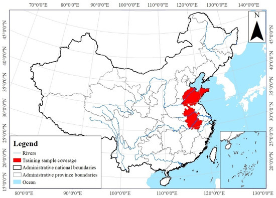
Figure 4.
The regions of the remote-sensing images.
Before feeding the images to the proposed modelling framework, several steps are implemented with the collected images in order to increase the efficiency of the network training and reduce uncertainty. As the remote shooting angles cannot remain constant and some disturbances are inevitable during the collection process, the position of objects such as buildings, roads, and rivers can be different. Therefore, we firstly checked the spatial consistency of these images and transformed them into the same format and projection. To achieve this, the metadata of two phases images were read to adjust the geospatial coordinates. Then we segmented the images based on the political boundaries of districts and counties (see Table 1), and the objects with changes in Phase II compared to Phase I, i.e., the changing samples, were marked manually. To address the need of monitoring to conserve water and soil and prevent floods, the most concerns in the demonstration case were focused on the changes in buildings, river channels or pipelines, newly constructed roads, and large-scaled alterations resulting from human activities such as excavation, occupation, dumping, or surface damage. Regarding the changing samples whose shape or location was changed, the boundary of the changing areas was marked while for the ones that newly appeared, the whole boundary was marked. Table 1 presents the changing samples extracted from the two provinces.

Table 1.
Manual annotation and collection list of change detection training samples.
Finally, the changing samples were cropped into multiple small segments via the toolkit, each with a size of 256 × 256, which were the inputs of the model. Additionally, we applied the toolkit to remove the interference samples which were located in unchanged regions and label the changed samples to enhance the efficiency of the training process. The input dataset of the model contained 2960 samples in total and was divided into three sets for training, validation, and testing, respectively. The division ratio of them was 7:2:1. The training set involving the majority of the samples served as the basic data for training the proposed ResNet18+Transformer model. The validation set representing 20% of the samples served as an intermediary checkpoint during the training, while the remaining 10% was the test set to evaluate the model capacity.
3.2. Training Result of the Proposed Framework
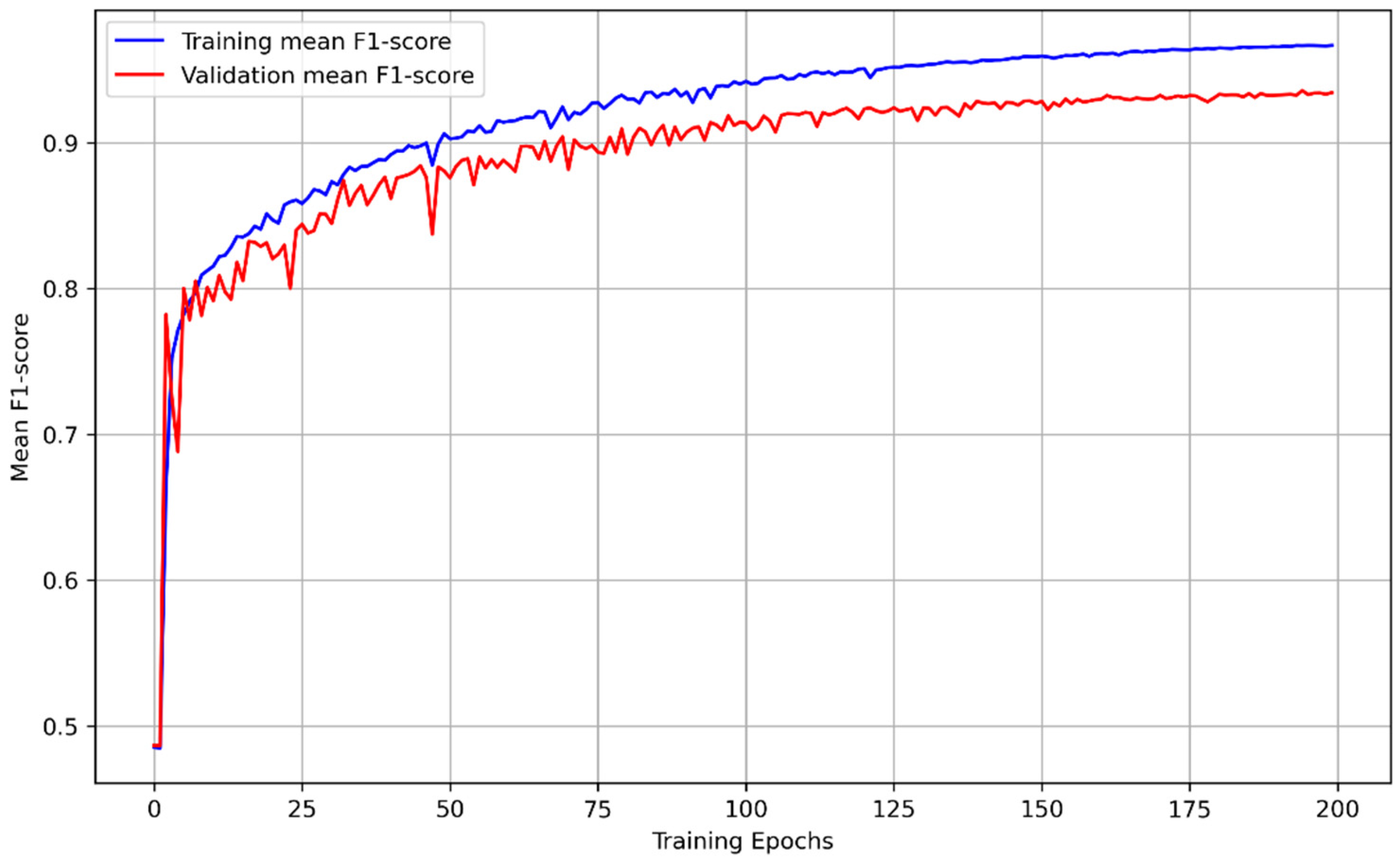
As mentioned above, the training of the proposed network model framework is took in the module of image cropping to segment the samples of Phase I and II with the size of 256 × 256, which have manually marked change regions on them. In order to minimize the overall loss, the training process was accompanied by an optimization algorithm that was used to adjust the network weights until the accuracy rate of the model converged to a high level. In this case, we utilized the stochastic gradient descent (SGD) algorithm for iterative learning, with the following settings: an initial learning rate of 0.01, maximum epochs of 200, linear decay for learning rate decay, every ‘step_size’ epochs for learning rate decay step, and a learning rate decay rate of 0.1. The training process was conducted on an NVIDIA GeForce RTX 4090; the mean F1-score on the training set and validation set over the epochs is presented in Figure 5.

Figure 5.
Training and validation mean F1-score of models for train epochs.
The training was finished after 200 epochs while the validation set was used to provide an unbiased evaluation of a model fit on the training set; the test set was used to provide a final evaluation of the model fit. During the training process, the model with the best fit kept updating based on its performance on the validation set, and the model with the highest mean F1-score in 200 epochs was selected as the final version of the model. The metrics of the changing regions (i.e., positive samples) for evaluating the performance and capacity of the model are presented in Table 2, where the overall accuracy of the model on the training, validation, and test sets is 0.99269, 0.98779, and 0.98764, respectively. Figure 6 is generated to visualize the testing results of the model by randomly selecting 24 samples. The rows of (a), (e), and (i) denote the samples of Phase 1 while (b), (f) and (j) are the corresponding same locations in Phase 2. The change detection results are depicted in (c), (g), and (k) respectively and (d), (h), and (l) demonstrate the ground truth which is the real change situation. It can be observed that the proposed model predicts the changing regions with both similar shape and size to the real situation, as evidenced by comparing the predictions (see Figure 6c,g,k) with their ground truth (see Figure 6d,h,l). These findings with the evaluation matrics suggest that the proposed model performed well on the test set.
Table 2.
Evaluation metrics on the training, validation, and test sets.
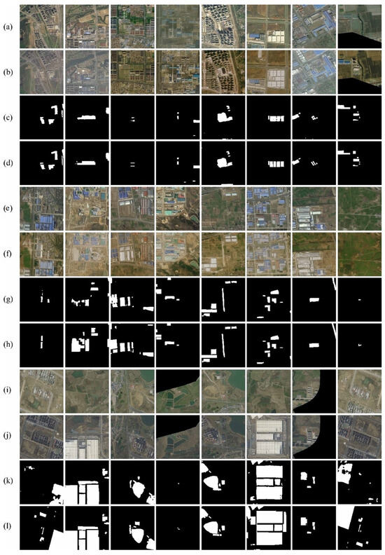
Figure 6.
Comparison of the predicted change regions with the ground truth on the test set where the color of white indicates the changes and black is unchanged. (a,e,i) denote the samples of Phase 1; while (b,f,j) are the samples of Phase 2 at the same locations; (c,g,k) denote the prediction by the model while (d,h,l) denote the ground truth which the real change situation.
Additionally, one notable observation is that compared to the ground truth which just roughly depict the boundary of the change areas such as a changing building, the prediction results by the proposed model are able to recognize more precise details in the edges and boundaries of the changing buildings. This could be attributed to the incorporation of the attention mechanism into the transformer architecture. The attention mechanism allows the model to concentrate on relevant features in space and their relationships, enabling it to effectively recognize the intricate details such as the building edges from the complex context. Therefore, the proposed model presents its potential ability to detect changes where precise details should be involved, for example, in detecting the changes in urban areas, the building boundaries could present the accurate scope of the changing areas.
4. Discussion
4.1. Performance Evaluation
To further evaluate the performance of the proposed modelling structure, we selected several advanced deep learning models which were applied to image pattern recognition to detect changes, including one convolution-based model, i.e., the bitemporal-FCN [27], and three attention-based models, i.e., the STANet-BAM [38], the STANet-PAM [38], and the SNUNet [48]. The characteristics of these four models and the proposed model are compared in Table 3.
Table 3.
The characteristics of the four models and the proposed model.
To implement these models, we used the open-source code with the default hyperparameters and the same input datasets (i.e., same training, validation, and test sets as the proposed model). Table 4 and Table 5 demonstrate the evaluation metrics of all the models on both the validation and test sets.
Table 4.
The performance of all models on the validation set where the highest scores are marked in bold.
Table 5.
The performance of all models on the test set where the highest scores are marked in bold.
Overall, the proposed model outperformed the other four models on both the test and validation sets. The Overall Accuracy, F1-score, and IoU of the proposed model consistently scored higher than those of other models, which indicates better efficacy in capturing and recognizing the changes within these high-resolution remote-sensing images. In particular, the F1-score of the proposed model on the test set is 8.7%, 1.8%, 4.2%, and 0.8% higher than the Bitemporal-FCN, STANet-BAM, STANet-PAM, and SNUNet, respectively. It means that the proposed model presented a significant improvement in the balance between identifying the positive samples (w.r.t. precision) and avoiding false positives (w.r.t. Recall), despite not achieving the highest values for these two single metrics.
However, the Bitemporal-FCN presents the highest precision of 0.94436 on the test set but achieves the lowest Recall of 0.65933 while the balance between them indicates by the F1-score was worse. It could be explained that the Bitemporal-FCN tends to act more conservatively in capturing all the positive samples, resulting in a higher likelihood of missing some actual positive samples.
In contrast, the proposed model leverages the advantage of the transformer structure and enhanced the capacity to extract semantic information effectively. Additionally, the integration of the transformer enables the model to capture the long-range dependencies and contextual relationships, contributing to superior performance. Compared with other developed attention mechanism models such as the STANet-BAM, STANet-PAM, and SNUNet, the architecture of the proposed model demonstrates a better capacity in extracting high-level semantic information as the interaction between the convolutional and transformer layers enhances the model’s capability to recognize and deal with the complex changes in remote-sensing images with high resolution.
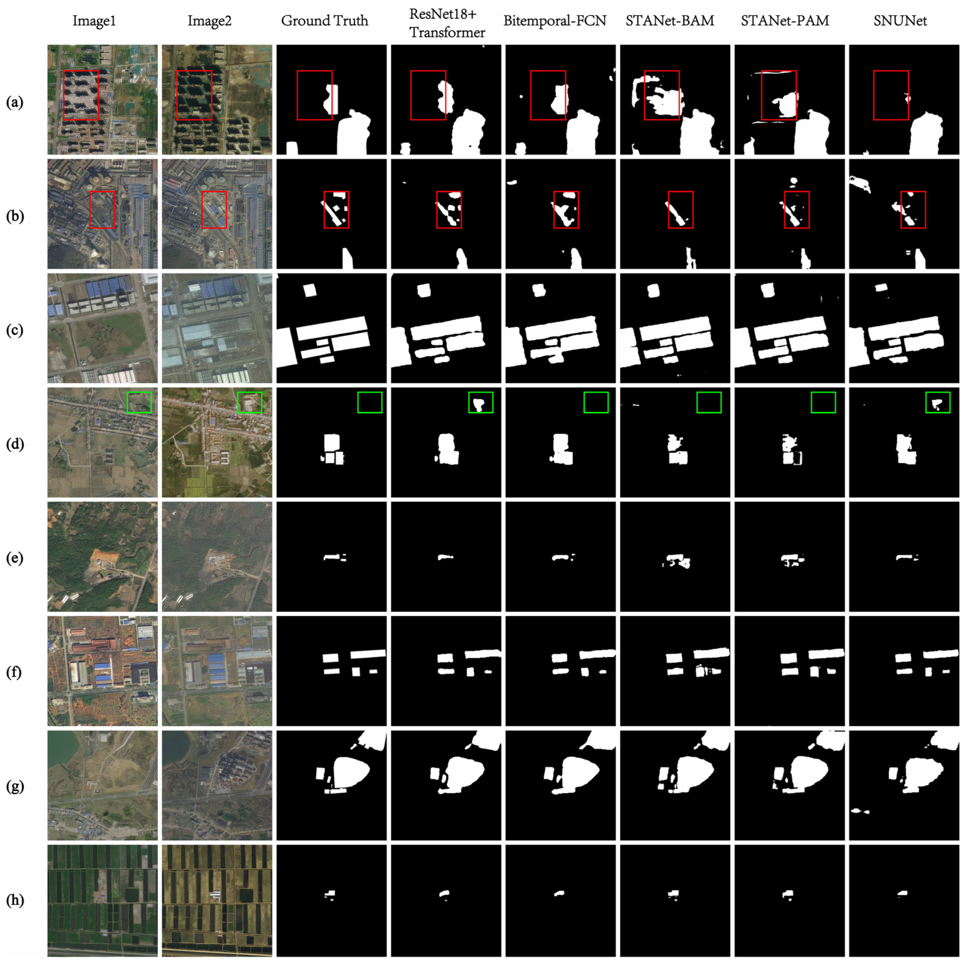
To visualize the comparison results, 16 test results were randomly selected and presented in Figure 7 and Figure 8. The color of white indicates the true positives that mean the real changing regions while the color of black indicates the true negatives that mean the real unchanged regions. All the detections are compared to the ground truth. To help visualization, the notable comparison is marked by red and green circles. The red circles represent precise change detection by the proposed models, whereas other models either detect additional areas or fail to identify certain areas. And the green circles indicate in-stances where ground truth missing marked change areas but successfully predicted by the models. As shown in Figure 7a, the prediction results of STANet-BAM, and STANet-PAM models contain many false positives (FP) and although the other three models have very few FP, SNUNet has more false negatives (FNs). This is consistent with the matrices presented in Table 4, where Precision of the STANet-BAM and STANet-PAM models on the test set is lower than the other three models. Generally, the proposed model presents a closer shape and size of the changing regions to the ground truth.
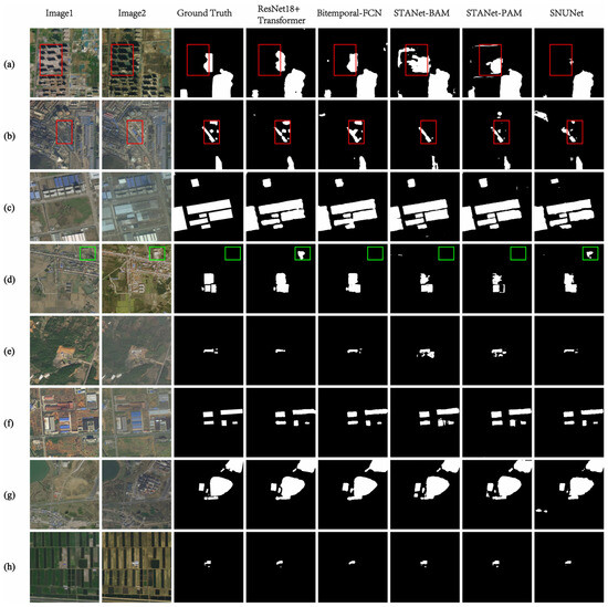
Figure 7.
Visualization results of different models where the 1st and 2nd columns are two phases of remote-sensing samples, the 3rd column is the ground truth, and the remaining columns are the changing regions predicted by the five models. (a–h) denote 8 pairs of samples randomly selected by the models.

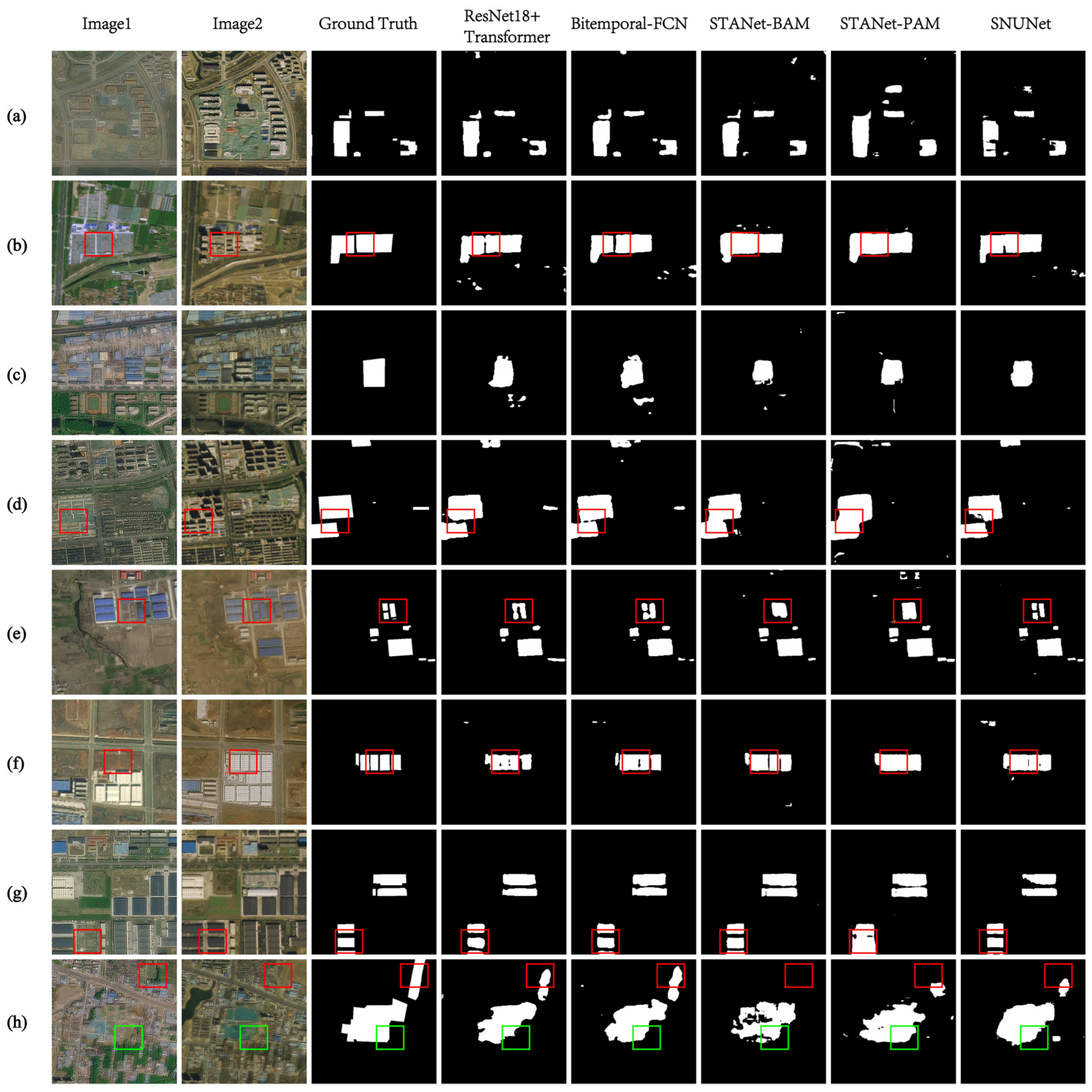
Figure 8.
Visualization results of different models where the 1st and 2nd columns are two phases of remote-sensing samples, the 3rd column is the ground truth and the remaining columns are the changing regions predicted by the five models. (a–h) denote 8 pairs of samples randomly selected by the models.
However, in Figure 8d, the proposed model recognized one more building than the other models except the SNUNet. The reason is that this building is missing marked in the ground truth samples but it can be clearly seen in Image 1 and 2. It can be concluded that the proposed model and SNUNet have better extrapolation and robustness. Moreover, in Figure 8b,d,f,g, STANet-BAM, and STANet-PAM models mark the boundary of the changing building overlapped with the adjacent objects if in close proximity. It results in the low Precision although Recall can be compensated to a certain extent. The proposed model can somehow overcome this problem by avoiding too many false negatives when Precision is high.
By comparing the performance of the proposed ResNet + Transformer model with the FCN-based and UNet-based models in detecting changes from high-resolution images, it is important to note that the image resolution can impact the applicability and detection accuracy of these deep learning methods. Since the receptive field of CNNs is determined by specific sizes of convolutional kernels and pooling layers, an image with finer resolutions contains numerous information where the actual receptive field of CNNs becomes relatively smaller. By incorporating transformers, the proposed structure enables capturing global semantic information within the context, thereby compensating for the limitations of CNN-based models. Therefore, the proposed model is less sensitive to image resolution, and demonstrates superior capability in dealing with high-resolution images or cases involving varying resolutions compared to the FCN-based and UNet-based models.
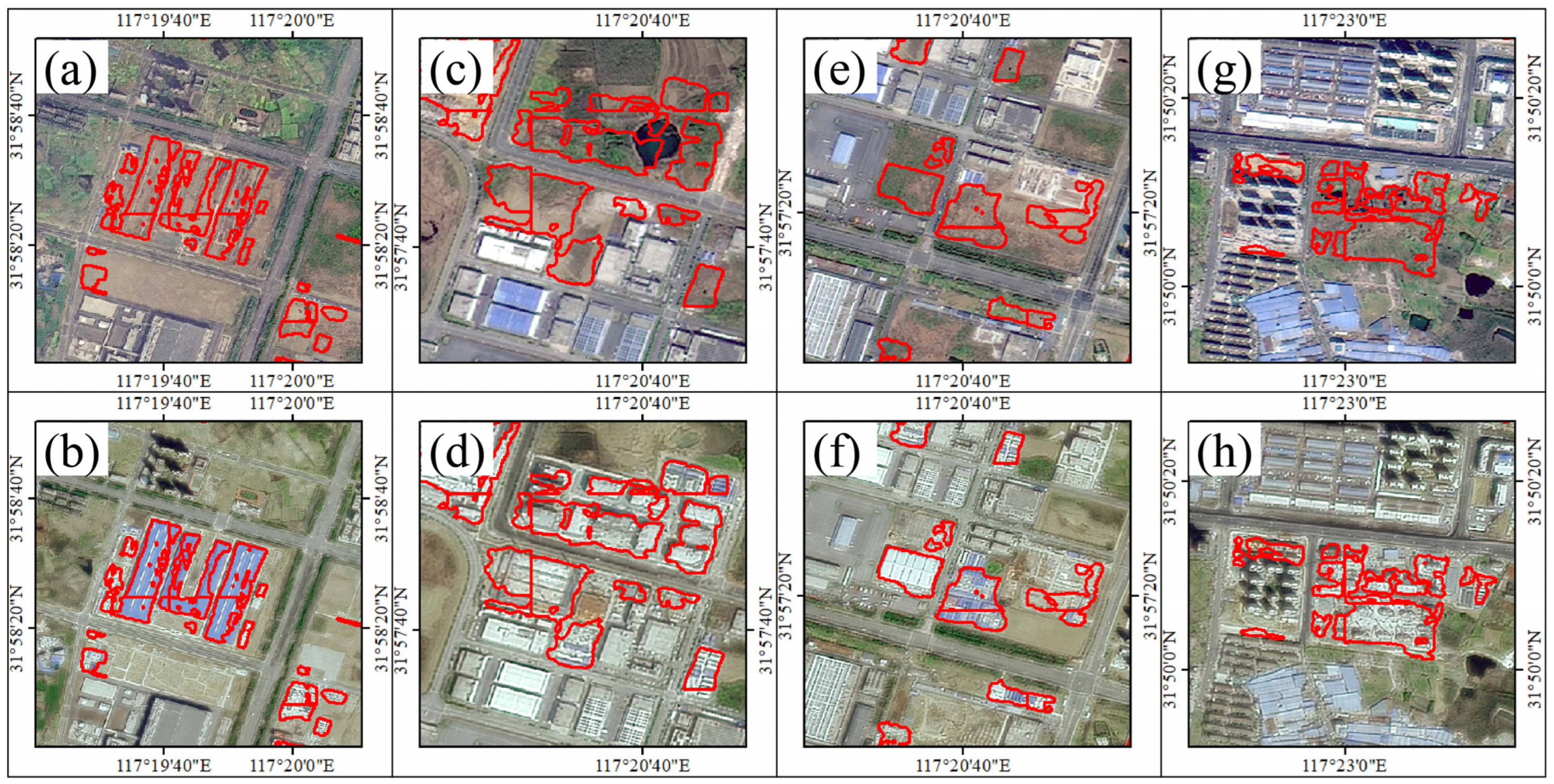
4.2. Application of ResNet18+Transformer Model
To further test the application of the proposed model, we collected remote-sensing images from another source which shows the surface changes in Yaohai District with the size of 62.8 km2 in 2022 and 2023. The preprocessing of the image was the same as with the demonstration case. To simplify the statistical analysis, only the regions greater than 1 km2 were used for discussion. In total, the model detected 835 change targets, of which 663 were correct and 172 were incorrect. The accuracy of the model in handling complex images in practical applications could be estimated at approximately 80%.
Figure 9 demonstrates several detection results in Yaohai District, which presents robust capability in effectively detecting the newly constructed objects upon open land.

Figure 9.
Some change detection results of the proposed model applied in Yaohai District. The area wrapped in red is the detection result predicted by the model in 2022 (a,c,e,g) and 2023 (b,d,f,h).
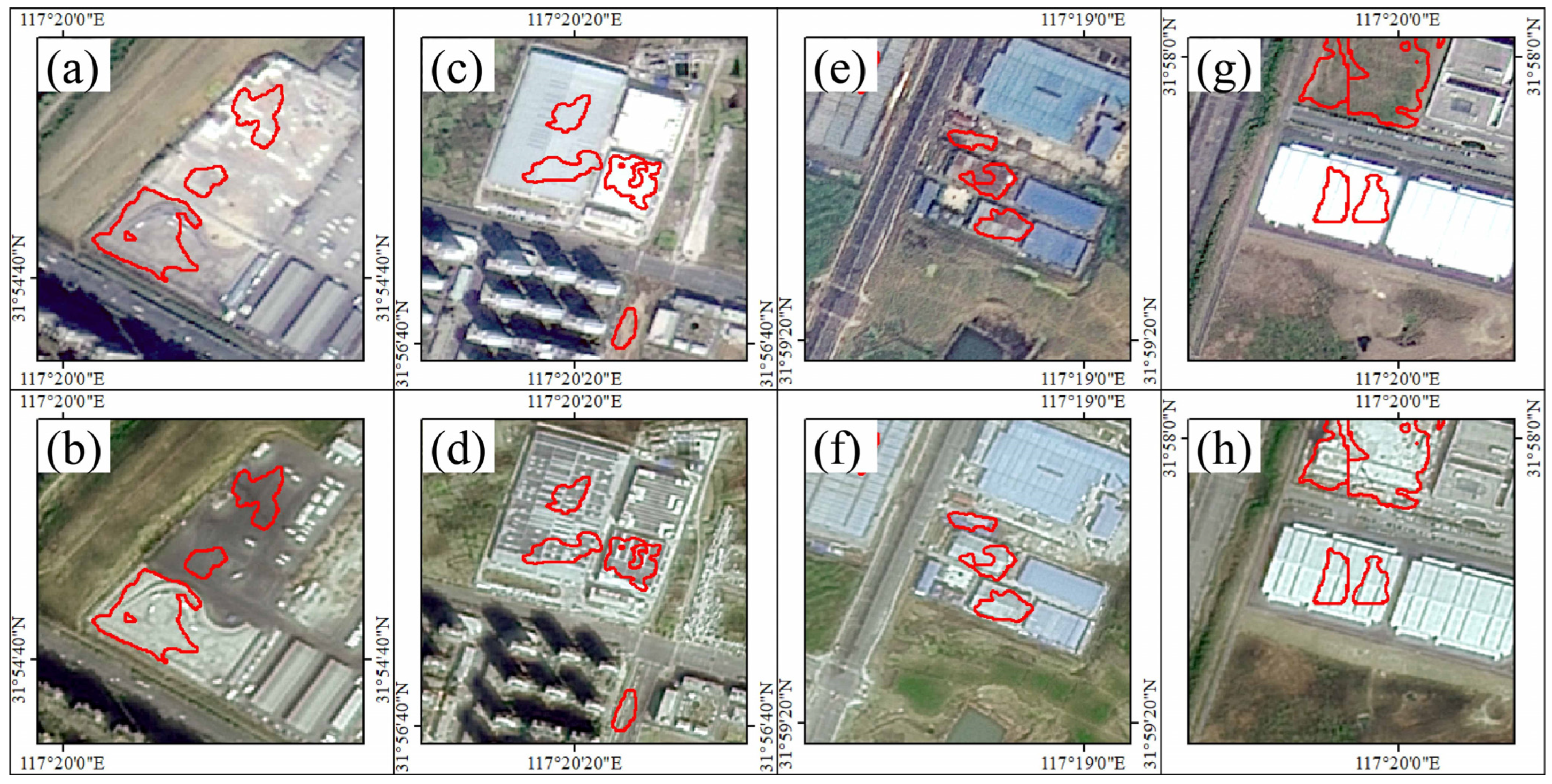
Figure 10 demonstrates some wrong detections generated by the proposed model, which are the regions detected as changed but not changing in semantics. In terms of the error group in Figure 10a,b, the reason could be attributed to the evident disparity in colour between the open spaces depicted in the two images. Referring to Figure 10c,d, since one shed roof of a factory was removed, the model tends to identify it as changed. And for Figure 10e,f, the mistake is due to the change in the colour of the roof. The one in Figure 10g,h can be attributed to the noise of too strong illumination, resulting in semantic errors in the original feature extraction in ResNet-18 although the model structure is designed to obtain the ability to mitigate such an effect.
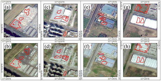
Figure 10.
Some error change detection regions in Yaohai District where the area wrapped in red is the detection result by the model in 2022 (a,c,e,g) and 2023 (b,d,f,h).
5. Conclusions
This paper proposes a new deep learning model called the ResNet18+Transformer model by combining a renovated Transformer and CNN to detect the changes from remote-sensing images with high resolution. To demonstrate the application of the proposed model, we trained the model with remote-sensing images of the Shandong and Anhui Provinces of China in 2021 and 2022 while one district of 2023 was used to evaluate the prediction accuracy of the trained model. Five widely-used matrices, i.e., the Overall Accuracy, F1-score, IoU, Precision, and Recall were employed to evaluate the performance of the developed architecture of the model and further compared with the other four advanced deep learning models (convention-based and attention-based) that were applied in change detection. Additionally, we also develop a toolkit to support image preprocessing including image cropping, result splicing, and vector conversion. The results can be concluded as follows.
- (1)
- Compared to fully convolutional neural networks, incorporating attention mechanisms can achieve better results since CNNs usually ignore the global information, resulting in limited handling with high-level semantic features at the global level.
- (2)
- Among attention networks, the Vision Transformer structure outperforms the pure multi-head attention since its unit structure can add a feed-forward network based on the self-attention mechanism to achieve channel-dimensional information interaction.
- (3)
- The proposed model outperforms both the convolution-based model and attention-based models in terms of Overall Accuracy, F1-score, and IoU since it combines the great capability of CNN on image feature extraction, and the ability to obtain global semantic information from the attention mechanism. It presents a significant improvement in the balance between identifying the positive samples and avoiding false positives in complex image change detection.
- (4)
- The proposed structure shows better extrapolation and robustness in handling complex images in practical applications with an approximately 80% accuracy in detecting changes in new testing sets (i.e., Yaohai District in 2022 and 2023).
Although the proposed model possesses strong robustness in the field of change detection, it can be sensitive to too strong illumination and color changes; mitigating the effect of illumination is still challenging in pattern recognition for all deep learning algorithms. Future research in the change detection model is expected to increase the resistance to strong illumination reflections and apparent color changes, for example, by developing a rectification mechanism to identify whether the changes are attributed to the noises.
The source code of the ResNet18+Transformer and the remote-sensing images processing toolkit are available on GitHub (https://github.com/yaoshunyu9401/CD_toolkit, accessed on 20 February 2024). The source code is provided subject to an MIT License. Use/fork of the code is subject to proper acknowledgement as stated on the web page of the model and toolkit.
Author Contributions
Conceptualization, S.Y. and H.W.; methodology, S.Y., H.W., Y.L. and D.C.; software, S.Y.; validation, S.Y., H.W. and Y.S.; investigation, S.Y.; resources, Y.S., T.S. and Q.L.; data curation, Y.S.; writing—original draft preparation, S.Y. and H.W.; writing—review and editing, S.Y. and H.W.; visualization, S.Y. and Y.S.; supervision, H.W.; project administration, C.L., T.S. and Q.L.; funding acquisition, H.W. All authors have read and agreed to the published version of the manuscript.
Funding
This research was funded by National Key R&D Program of China, Grant No: 2023YFC3006700.
Data Availability Statement
The dataset contains remote-sensing images of two districts and counties in 2022 and 2023, and the IWHR_data dataset is also included in the link. The dataset sharing link is as follows: https://pan.baidu.com/s/1lh1yuX_DC7M9tpKl2S_s8A (accessed on 23 March 2024) Extraction code: 4cix.
Acknowledgments
The authors would like to thank the Monitoring Center of Soil and Water Conservation, Ministry of Water Resources of the People’s Republic of China for providing the remote-sensing images for the demonstration case.
Conflicts of Interest
The authors declare that they have no known competing financial interests or personal relationships that could have appeared to influence the work reported in this paper.
References
- Zhang, H.; Wang, Z. Human activities and natural geographical environment and their interactive effects on sudden geologic hazard: A perspective of macro-scale and spatial statistical analysis. Appl. Geogr. 2022, 143, 102711. [Google Scholar] [CrossRef]
- Gill, J.C.; Malamud, B.D. Anthropogenic processes, natural hazards, and interactions in a multi-hazard framework. Earth-Sci. Rev. 2017, 166, 246–269. [Google Scholar] [CrossRef]
- Rahmati, O.; Golkarian, A.; Biggs, T.; Keesstra, S.; Mohammadi, F.; Daliakopoulos, I.N. Land subsidence hazard modeling: Machine learning to identify predictors and the role of human activities. J. Environ. Manag. 2019, 236, 466–480. [Google Scholar] [CrossRef] [PubMed]
- Shine, K.P.; de Forster, P.M. The effect of human activity on radiative forcing of climate change: A review of recent developments. Glob. Planet. Chang. 1999, 20, 205–225. [Google Scholar] [CrossRef]
- Trenberth, K.E. Climate change caused by human activities is happening and it already has major consequences. J. Energy Nat. Resour. Law 2018, 36, 463–481. [Google Scholar] [CrossRef]
- Liu, Y.; Huang, Y.; Wan, J.; Yang, Z.; Zhang, X. Analysis of human activity impact on flash floods in China from 1950 to 2015. Sustainability 2020, 13, 217. [Google Scholar] [CrossRef]
- Wang, F.; Mu, X.; Li, R.; Fleskens, L.; Stringer, L.C.; Ritsema, C.J. Co-evolution of soil and water conservation policy and human–environment linkages in the Yellow River Basin since 1949. Sci. Total Environ. 2015, 508, 166–177. [Google Scholar] [CrossRef] [PubMed]
- Xitao, H.; Siyu, C.; Yu, Z.; Han, Z.; Xiaofeng, Y.; Pengtao, J.; Liyuan, X. Study on Dynamic Monitoring Technology of Soil and Water Conservation in Construction Projects using Multi-source Remote Sensing Information. J. Phys. Conf. Ser. 2021, 1848, 012055. [Google Scholar] [CrossRef]
- Li, J.; Pei, Y.; Zhao, S.; Xiao, R.; Sang, X.; Zhang, C. A review of remote sensing for environmental monitoring in China. Remote Sens. 2020, 12, 1130. [Google Scholar] [CrossRef]
- Bovolo, F.; Bruzzone, L.; Marconcini, M. A Novel Approach to Unsupervised Change Detection Based on a Semisupervised SVM and a Similarity Measure. IEEE Trans. Geosci. Remote Sens. 2008, 46, 2070–2082. [Google Scholar] [CrossRef]
- Lu, D.; Weng, Q. A survey of image classification methods and techniques for improving classification performance. Int. J. Remote Sens. 2007, 28, 823–870. [Google Scholar] [CrossRef]
- Hussain, M.; Chen, D.; Cheng, A.; Wei, H.; Stanley, D. Change detection from remotely sensed images: From pixel-based to object-based approaches. ISPRS J. Photogramm. Remote Sens. 2013, 80, 91–106. [Google Scholar] [CrossRef]
- Pal, M.; Mather, P.M. An assessment of the effectiveness of decision tree methods for land cover classification. Remote Sens. Environ. 2003, 86, 554–565. [Google Scholar] [CrossRef]
- Soille, P.; Vogt, P. Morphological segmentation of binary patterns. Pattern Recognit. Lett. 2009, 30, 456–459. [Google Scholar] [CrossRef]
- Dalal, N.; Triggs, B. Histograms of oriented gradients for human detection. In Proceedings of the IEEE Computer Society Conference on Computer Vision and Pattern Recognition (CVPR), San Diego, CA, USA, 20–25 June 2005; pp. 886–893. [Google Scholar]
- Ke, Y.; Sukthankar, R. PCA-SIFT: A more distinctive representation for local image descriptors. In Proceedings of the IEEE Computer Society Conference on Computer Vision and Pattern Recognition (CVPR), Washington, DC, USA, 27 June–2 July 2004; pp. 506–513. [Google Scholar]
- Shi, W.; Zhang, M.; Zhang, R.; Chen, S.; Zhan, Z. Change Detection Based on Artificial Intelligence: State-of-the-Art and Challenges. Remote Sens. 2020, 12, 1688. [Google Scholar] [CrossRef]
- LeCun, Y.; Bengio, Y.; Hinton, G. Deep learning. Nature 2015, 521, 436–444. [Google Scholar] [CrossRef]
- Krizhevsky, A.; Sutskever, I.; Hinton, G.E. Imagenet classification with deep convolutional neural networks. Adv. Neural Inf. Process. Syst. 2012, 25, 1097–1105. [Google Scholar] [CrossRef]
- Deng, J.; Dong, W.; Socher, R.; Li, L.-J.; Li, K.; Fei-Fei, L. Imagenet: A large-scale hierarchical image database. In Proceedings of the IEEE Conference on Computer Vision and Pattern Recognition (CVPR), Miami, FL, USA, 20–25 June 2009; pp. 248–255. [Google Scholar]
- Szegedy, C.; Liu, W.; Jia, Y.; Sermanet, P.; Reed, S.; Anguelov, D.; Erhan, D.; Vanhoucke, V.; Rabinovich, A. Going deeper with convolutions. In Proceedings of the IEEE Conference on Computer Vision and Pattern Recognition (CVPR), Boston, MA, USA, 7–12 June 2014; pp. 1–9. [Google Scholar]
- Simonyan, K.; Zisserman, A. Very Deep Convolutional Networks for Large-Scale Image Recognition. In Proceedings of the International Conference on Learning Representations (ICLR), Banff, AB, Canada, 14–16 April 2014. [Google Scholar]
- Krizhevsky, A.; Sutskever, I.; Hinton, G.E. ImageNet classification with deep convolutional neural networks. Commun. ACM 2017, 60, 84–90. [Google Scholar] [CrossRef]
- He, K.; Zhang, X.; Ren, S.; Sun, J. Identity Mappings in Deep Residual Networks. In Proceedings of the European Conference on Computer Vision (ECCV), Amsterdam, The Netherlands, 11–14 October 2016. [Google Scholar]
- Chen, J.; Yuan, Z.; Peng, J.; Chen, L.; Huang, H.; Zhu, J.; Liu, Y.; Li, H. DASNet: Dual Attentive Fully Convolutional Siamese Networks for Change Detection in High-Resolution Satellite Images. IEEE J. Sel. Top. Appl. Earth Observ. Remote Sens. 2021, 14, 1194–1206. [Google Scholar] [CrossRef]
- Zhang, M.; Xu, G.; Chen, K.; Yan, M.; Sun, X. Triplet-based semantic relation learning for aerial remote sensing image change detection. IEEE Geosci. Remote Sens. Lett. 2018, 16, 266–270. [Google Scholar] [CrossRef]
- Zhang, M.; Shi, W. A Feature Difference Convolutional Neural Network-Based Change Detection Method. IEEE Trans. Geosci. Remote Sens. 2020, 58, 7232–7246. [Google Scholar] [CrossRef]
- Liu, Y.; Pang, C.; Zhan, Z.; Zhang, X.; Yang, X. Building change detection for remote sensing images using a dual-task constrained deep siamese convolutional network model. IEEE Geosci. Remote Sens. Lett. 2020, 18, 811–815. [Google Scholar] [CrossRef]
- Zhang, C.; Yue, P.; Tapete, D.; Jiang, L.; Shangguan, B.; Huang, L.; Liu, G. A deeply supervised image fusion network for change detection in high resolution bi-temporal remote sensing images. ISPRS J. Photogramm. Remote Sens. 2020, 166, 183–200. [Google Scholar] [CrossRef]
- Kalinaki, K.; Malik, O.A.; Ching Lai, D.T. FCD-AttResU-Net: An improved forest change detection in Sentinel-2 satellite images using attention residual U-Net. Int. J. Appl. Earth Obs. Geoinf. 2023, 122, 103453. [Google Scholar] [CrossRef]
- Song, L.; Xia, M.; Jin, J.; Qian, M.; Zhang, Y. SUACDNet: Attentional change detection network based on siamese U-shaped structure. Int. J. Appl. Earth Obs. Geoinf. 2021, 105, 102597. [Google Scholar] [CrossRef]
- Wang, X.; Yan, X.; Tan, K.; Pan, C.; Ding, J.; Liu, Z.; Dong, X. Double U-Net (W-Net): A change detection network with two heads for remote sensing imagery. Int. J. Appl. Earth Obs. Geoinf. 2023, 122, 103456. [Google Scholar] [CrossRef]
- Cheng, X.; Zhang, M.; Lin, S.; Li, Y.; Wang, H. Deep Self-Representation Learning Framework for Hyperspectral Anomaly Detection. IEEE Trans. Instrum. Meas. 2024, 73, 5002016. [Google Scholar] [CrossRef]
- Lin, S.; Zhang, M.; Cheng, X.; Shi, L.; Gamba, P.; Wang, H. Dynamic Low-Rank and Sparse Priors Constrained Deep Autoencoders for Hyperspectral Anomaly Detection. IEEE Trans. Instrum. Meas. 2024, 73, 2500518. [Google Scholar] [CrossRef]
- Peng, X.; Zhong, R.; Li, Z.; Li, Q. Optical Remote Sensing Image Change Detection Based on Attention Mechanism and Image Difference. IEEE Trans. Geosci. Remote Sens. 2021, 59, 7296–7307. [Google Scholar] [CrossRef]
- Jiang, H.; Hu, X.; Li, K.; Zhang, J.; Gong, J.; Zhang, M. PGA-SiamNet: Pyramid Feature-Based Attention-Guided Siamese Network for Remote Sensing Orthoimagery Building Change Detection. Remote Sens. 2020, 12, 484. [Google Scholar] [CrossRef]
- Yin, H.; Weng, L.; Li, Y.; Xia, M.; Hu, K.; Lin, H.; Qian, M. Attention-guided siamese networks for change detection in high resolution remote sensing images. Int. J. Appl. Earth Obs. Geoinf. 2023, 117, 103206. [Google Scholar] [CrossRef]
- Chen, H.; Shi, Z. A Spatial-Temporal Attention-Based Method and a New Dataset for Remote Sensing Image Change Detection. Remote Sens. 2020, 12, 1662. [Google Scholar] [CrossRef]
- Cui, F.; Jiang, J. MTSCD-Net: A network based on multi-task learning for semantic change detection of bitemporal remote sensing images. Int. J. Appl. Earth Obs. Geoinf. 2023, 118, 103294. [Google Scholar] [CrossRef]
- Chen, H.; Qi, Z.; Shi, Z. Remote sensing image change detection with transformers. IEEE Trans. Geosci. Remote Sens. 2021, 60, 5402711. [Google Scholar] [CrossRef]
- Vaswani, A.; Shazeer, N.; Parmar, N.; Uszkoreit, J.; Jones, L.; Gomez, A.N.; Kaiser, L.; Polosukhin, I. Attention is all you need. In Proceedings of the International Conference on Neural Information Processing Systems (NeurIPS), Long Beach, CA, USA, 4–9 December 2017. [Google Scholar]
- Dosovitskiy, A.; Beyer, L.; Kolesnikov, A.; Weissenborn, D.; Zhai, X.; Unterthiner, T.; Dehghani, M.; Minderer, M.; Heigold, G.; Gelly, S. An image is worth 16 × 16 words: Transformers for image recognition at scale. In Proceedings of the International Conference on Learning Representations (ICLR), Addis Ababa, Ethiopia, 26–30 April 2020. [Google Scholar]
- Wang, H.; Xuan, Y. A Spatial Pattern Extraction and Recognition Toolbox Supporting Machine Learning Applications on Large Hydroclimatic Datasets. Remote Sens. 2022, 14, 3823. [Google Scholar] [CrossRef]
- He, K.; Zhang, X.; Ren, S.; Sun, J. Deep residual learning for image recognition. In Proceedings of the IEEE Conference on Computer Vision and Pattern Recognition (CVPR), Las Vegas, NV, USA, 27–30 June 2016; pp. 770–778. [Google Scholar]
- Ho, Y.; Wookey, S. The real-world-weight cross-entropy loss function: Modeling the costs of mislabeling. IEEE Access 2019, 8, 4806–4813. [Google Scholar] [CrossRef]
- Monard, M.C.; Batista, G. Learning with skewed class distributions. Adv. Log. Artif. Intell. Robot. 2002, 85, 173–180. [Google Scholar]
- Redmon, J.; Divvala, S.; Girshick, R.; Farhadi, A. You only look once: Unified, real-time object detection. In Proceedings of the Proceedings of the IEEE Conference on Computer Vision and Pattern Recognition, Las Vegas, NV, USA, 27–30 June 2016; pp. 779–788. [Google Scholar]
- Fang, S.; Li, K.; Shao, J.; Li, Z. SNUNet-CD: A Densely Connected Siamese Network for Change Detection of VHR Images. IEEE Geosci. Remote Sens. Lett. 2021, 19, 8007805. [Google Scholar] [CrossRef]
- Zhou, Z.; Rahman Siddiquee, M.M.; Tajbakhsh, N.; Liang, J. Unet++: A nested u-net architecture for medical image segmentation. In Deep Learning in Medical Image Analysis and Multimodal Learning for Clinical Decision Support; Springer: Berlin/Heidelberg, Germany, 2018; pp. 3–11. [Google Scholar]


Disclaimer/Publisher’s Note: The statements, opinions and data contained in all publications are solely those of the individual author(s) and contributor(s) and not of MDPI and/or the editor(s). MDPI and/or the editor(s) disclaim responsibility for any injury to people or property resulting from any ideas, methods, instructions or products referred to in the content. |
© 2024 by the authors. Licensee MDPI, Basel, Switzerland. This article is an open access article distributed under the terms and conditions of the Creative Commons Attribution (CC BY) license (https://creativecommons.org/licenses/by/4.0/).