Spatio-Temporal Changes and Driving Forces Analysis of Urban Open Spaces in Shanghai between 1980 and 2020: An Integrated Geospatial Approach

Abstract

Although there is extensive research demonstrating the significant loss and fragmentation of urban spaces caused by rapid urbanization, to date, no empirical research in Shanghai has investigated the spatiotemporal dynamics of urban open spaces using a comprehensive set of integrated geospatial techniques based on long-sequence time series. Based on the Google Earth Engine (GEE) platform and using the Random Forest (RF) classifier, multiple techniques, namely landscape metrics, trend analysis, open space ratio, transition matrix, Normalized Difference Vegetation Index (NDVI), and fractal dimension analysis, were applied to analyze the Landsat satellite data. Next, Geographic Detector (GeoDetector) methods were used to investigate the driving forces of such spatial variations. The results showed that (1) the RF classification algorithm, supported by the GEE, can accurately and quickly obtain a research object dataset, and that calculating the optimal spatial grain size for open space pattern was 70 m; (2) open spaces exhibited declining and contracting trends; and open spaces in the city experienced a decline from 91.83% in 1980 to 69.63% in 2020. Meanwhile, the degree of open spaces in each district increased to different extents, whilst connectivity markedly decreased. Furthermore, the open space of city center districts showed the lowest rate of decrease, with open space patterns fragmenting due to encroaching urbanization; (3) the contribution of socioeconomic factors to the spatial–temporal changes in open space continually has increased over the past 40 years, and were also higher than natural geographic factors to some extent. Apart from offering policy insights guiding the future spatial planning and development of the city, this paper has contributions from both methodological and empirical perspectives. Based on integrated remote sensing and geographic information science (GIS) techniques, this paper provides updated evidence and a clearer understanding of the spatiotemporal variations in urban spaces and their influencing mechanisms in Shanghai.

1. Introduction

The speed of urbanization has increased faster than ever before in history: it is predicted that as of 2025, 65% of the world’s population will live in urban areas [1]. A corollary of urbanization and the associated build-up of areas is the shrinking of urban open space (UOS), which is to the detriment of ecosystems and the environment [2]. The majority of the environmental impacts associated with urbanization relate to the destruction of open green space, which produces a myriad of negative impacts, including but not limited to habitat destruction, biodiversity reduction, and disruption of the urban ecosystem’s processes and structures [3]. Contrastingly, these impacts can be mitigated to some extent by the presence of open green spaces, as can be seen with how they regulate the urban heat island effect [4], energy flows [5], and water and atmospheric pollution, respectively [6]. In addition to its various environmental benefits, the enhancement of open green space also creates recreational opportunities for urban residents in locations that both provide aesthetic enjoyment and can boost physical and mental health [7].

As a global megacity, Shanghai continues to rapidly urbanize. However, a number of urbanization-related issues jeopardize the city’s sustainable development ambitions and take up valuable urban open green space, such as population growth, short-term high-density investment, and the continually increasing plot ratios and building densities. In the forty years covered in this study (1980–2020), Shanghai’s government have designed and implemented an urban master plan, which was then updated to cover the periods of 1986–2000, 1999–2020, and 2017–2035. It must be highlighted that each of the three master plans included content relating to urban open green space.

To date, few studies have explored Shanghai’s spatiotemporal dynamics, with even fewer conducting an investigation across different periods in the city’s history [8,9,10,11]. For instance, Wu et al. [9] have probed the temporal and spatial changes that took place in Shanghai’s urban green spaces between 1980 and 2015, with a particular focus on the underlying forces driving the observed changes. Prior to this, Li et al. [10] have looked into the Shanghai metropolitan area’s spatiotemporal dynamics from 1989 to 2005. Though studies such as these have made valuable contributions, there has yet to be a study considering the theme of “open space” over a long research period. In recent years, the Google Earth Engine (GEE) has been the subject of much academic attention, especially GEE-based research into machine learning and land cover [12]. Even so, there has yet to be a study of Shanghai using the optimum grain size to achieve high-accuracy mapping. Similarly, satellite remote sensing techniques and geographical information systems (GISs) have frequently been used to monitor land-use changes over time [13]. Xu and Cui [14] have monitored how Suzhou’s green spaces have changed over time using a range of landscape metrics, paying particular attention to the spaces’ scales and spatial layouts. Elsewhere, Kong and Nakagoshi [15] have used landscape metrics to quantify landscape patterns, whilst Liu et al. [16] have employed a fractal dimension methodology to analyze the evolution of UGS’s spatiotemporal characteristics. More recently, Xiao et al. [17] have relied on a transfer matrix and remote sensing images to research green space development in Zhengdong New District, China. To date, no study has used an integrated analysis approach to quantitatively characterize open space changes. Integrating approaches that are based on different perspectives can provide a more holistic understanding of and responses to UOS changes.

It must be stressed that “open space” is a worthy research subject. Specifically, open space refers to external urban public space, including but not limited to roads, squares, natural scenery, public green space, and rest space [18]. For present purposes, open spaces are those spaces dominated by a “natural” environment. Applying this logic, most UOSs are green spaces, though that does not preclude them from including other kinds of open areas. This concept has a wide meaning that covers both ‘green space’ and ‘public space’. Accordingly, applying the definition used in this study, open space includes farmland, forests, grassland, and waterbodies, whilst non-open space includes built-up areas and unused land. However, when carrying out land-cover classification, simple algorithms are used to carry out traditional remote sensing image classification methods. Prime examples of this are visual interpretation and statistics-based classification methods [19]. The classification accuracy of these methods decreases where foreign bodies are present. Newly developed artificial intelligence (AI) classification methods that utilize algorithms, most notably the Random Forest method, are more accurate in their classifications than the methods that preceded them. Fortunately, the GEE platform features large-scale remote sensing datasets, spatial calculation, and analysis functions to facilitate work of the kind detailed above.

Under the growing pressure to provide additional housing and business premises in urban areas, existing urban green spaces are being altered faster and on a greater scale than before. Urbanization precipitates land-use pattern changes, causing the occupation of green spaces [11,20]. Xu and Cui [14] have concluded that the urban green spaces of different districts have changed in different ways depending on their geographical location. Yuan et al. [4] show that climatic factors have dominant impacts on urban green space variation. Among the climatic variables, precipitation has the largest relative importance. This is because precipitation plays key roles in vegetation distribution patterns in both natural and urban ecosystems.

While regarding the studies conducted on the influencing factors analysis method, the use of qualitative methods to conduct policy-driven impacts has been mentioned in most previous efforts [20,21,22]. For instance, Wu et al. [9] have mainly focused the driving effect of policies on the changes in urban green spaces in Shanghai between 1980 and 2015 by related policy and planning documents analysis. Additionally, the selection of quantitative evaluation methods for driving forces is still relatively more common with statistical analysis, namely logistic regression models [23], GeoDetector [24], geographically weighted regression (GWR) [25], and analytic hierarchy process (AHP) [26]. Wu et al. [27] have studied partial least square regression to understand the contribution of the main socioeconomic driving factors in Shanghai urbanization research. Unlike prior studies, as a new spatial statistical method, the geographic detector method can be used for detecting spatial variations and revealing driving factors and was proposed by Wang Jinfeng [24]. It has also acquired broad applications in explaining drivers [28,29]. Also, the combination of quantitative and qualitative evaluation, from natural factors, socioeconomic factors, climate factors, and policy factors to comprehensive analysis of the driving force of UGS changes, is relatively rare.

As detailed above, this research investigates the spatiotemporal dynamics of open space in Shanghai by employing data from the past 40 years. Specifically, an integrative approach is adopted that is premised on geographic information science (GIS) and remote sensing techniques. Moreover, it is necessary to fully comprehend the dynamic characteristics of spaces to redress the conflict between urban land expansion and open green space protection, and we apply the Geographic Detector (GeoDetector) methods to explore the factors impacting on urban open space change processes in the study area. On this basis, the results of this study will be of great practical significance for rationally planning land resources, which in turn will promote healthy urban development as well as sustainable and enduring ecological security. We endeavor to address the subsequent three questions:

(1)

How can we produce high-accuracy, high-precision open space mapping over long time series in Shanghai?

(2)

What have the spatio-temporal urban open space change dynamics been in Shanghai over the 40 years?

(3)

What were the main factors driving urban open space changes in Shanghai during the period of 1980–2020?

2. Study Area and Data Description

2.1. Study Area

Covering an urban area of 6340.5 km², Shanghai (30°40′–31°53′N and 120°51′–122°12′E) is a coastal megacity located in eastern China [30]. As a central feature in the urban agglomeration of the Yangtze River Delta urban agglomeration, Shanghai is a hub of commerce, finance, innovation, economics, and transportation in China. As of 2020, Shanghai is home to 24.89 million residents, making it the urban area with the highest population in China. Interestingly, the city’s gross domestic product (GDP) has exploded over the last forty years, rapidly rising from RMB 30 billion in 1980 to RMB 480 billion in 2000, before RMB 3900 billion of research in 2020, a close to 130-fold increase in 40 years [30].

The city’s urban area is made up of 16 districts, which are divided into three zones: the city center, the suburbs, and the islands. The city center covers seven districts (Jing’an, Changning, Huangpu, Hongkou, Putuo, Yangpu, Xuhui), the suburbs eight (Jiading, Baoshan, Pudong, Minhang, Qingpu, Songjiang, Jinshan, and Fengxian), and the three islands (Chongming Island, Changxing Island, and Hengsha Island) (Figure 1). The 2017–2035 Shanghai Master Plan emphasizes the need to build a more sustainable eco-city characterized by green spaces and low-carbon infrastructure. With this goal in mind, research into Shanghai’s urban open green space pattern has assumed renewed importance.

2.2. Data Description

This study used land-use datasets consisting of Landsat OLI (National Aeronautics and Space Administration, Washington, DC, USA) and Landsat TM/ETM (National Aeronautics and Space Administration, Washington, DC, USA) images pertaining to the following years: 1980, 1990, 2000, 2010, and 2020. Moreover, the types of land use employed for classification in Shanghai were taken from a previous study [11], and are aligned with the Chinese Academy of Sciences’ land-use classification criteria [31]. However, the change in land use into open space or non-open space was reclassified to provide more detail on changes to use as cropland, forest, grassland, water, built area, or barren land (

Table 1. The land-use/land-cover classification [32].

Attributes	Category	Explanation
Open space	Cropland	Agricultural land and permanent crops, including vineyards, hop fields, gardens and orchards
	Forest	Land for growing trees, shrubs, and bamboo, as well as coastal mangrove forest
	Grassland	Land for growing grasses, sedge, and shrubs
	Water	Natural land and water conservancy facilities
Non-open space	Built area	Lands used for urban and rural settlements, Factories, and transportation facilities.
	Unused land	Lands that are not put into practical used or are difficult to use

). The remotely sensed images used here relate to the appropriate period and are almost free of clouds. To be precise, in GEE, images were taken between June and September from 1980 to 2010, whilst the images for 2020 were taken from Landsat 8 OLI. Meanwhile, the image preprocessing included the following steps: multispectral remote sensing image synthesis, followed by a geometric correction, and finally image clipping of the selected area of study.

According to existing research [33,34], the influencing factors of the spatial–temporal change in green space have included climatic factors, socioeconomic determinants, and natural geographic factors. All the factors selected were proved to affect the change in green space. Thus, 19 exploratory variables related to the change in open spaces were selected. See

Table 2. Selected variables used to study the factors influencing urban open spaces.

Variable Category	Code	Variable Name	Sources
Dependent variable	Y	Open space	Extracted from remote sensing images [35]
Natural geographic factors	X1	Normalized Difference Vegetation Index (NDVI)	Extracted from remote sensing images [35]
	X2	DEM	[35]
	X3	Slope	[35]
	X4	Soil moisture (SOIL)	[36]
	X5	Runoff (RO)	[36]
Socioeconomic factors	X6	Gross domestic product (GDP)	[37]
	X7	Population density (POP)	[38]
	X8	Carbon emission density (CE)	[39]
	X9	Electricity consumption (EC)	[37]
Climatic factors	X10	Precipitation (PR)	[36]
	X11	Maximum temperature (TMMX)	[36]
	X12	Minimum temperature (TMMN)	[36]
	X13	Vapor pressure difference (VPD)	[36]
	X14	Actual evapotranspiration (AET)	[36]
	X15	Solar radiation (SRAD)	[36]
	X16	Potential evapotranspiration (PET)	[36]
	X17	Palmer Drought Severity Index (PDSI)	[36]
	X18	Atmospheric pressure (VAP)	[36]
	X19	Climate water deficit (DEF)	[36]

.

3. Methods

The present study’s methodology consists of three distinct parts: the first used RF classifier-based GEE to carry out land-use classification, before calculating the optimum granularity to obtain high-accuracy classification images. The second used six methods to analyze the spatio-temporal changes in open space in Shanghai over the study period. The third explored the driving forces of open space changes based on factor detectors. The brief details of the methodology applied in this research are presented in Figure 2.

3.1. Google Earth Engine, Random Forest, Optimal Granularity

As noted above, the methodological procedures deployed in this study were based on the Google Earth Engine (GEE) cloud platform, which is free to use. Figure 2 outlines the study workflow, whilst the subsections below elaborate on the specific procedures involved. The GEE platform is an easy-to-use, web-based, open-source cloud computing tool that provides access to and processing, interpretation, and analysis of big geodata [12]. First launched in 2010, the GEE platform now offers access to the data collection of multiple satellites, including the most widely used dataset, namely, the Landsat mission [40]. To be precise, the data collection accessible through GEE runs from the 1970s through to today [41]. GEE was employed here to both produce Landsat image composites for 10-year intervals and perform machine learning classification. Random Forest (RF) is the most used machine learning classifier [42] on GEE [41]. RF employs a decision tree method and incorporates an ensemble learning approach based on boosting and bagging procedures to classify satellite image pixels to carry out its work. These techniques combine various models and set them to solve the same problem, elevating the classifier’s classification accuracy.

From a process perspective, RF utilizes a bagging operation to create multiple decision trees (ntree) based on a training data subset selected at random. Using a bootstrapped sample from the training dataset, each tree is independently grown to its maximum size (note that no pruning is carried out). Subsequently, each node is split apart based on the best input variable from a specific subset (mtry) [43]. To carry out the actual classification prediction, the most popular voted class from each tree predictor is selected. It should be highlighted that RF classification accuracy is shaped by two key parameters: the number of trees (Ntree) and the number of features (Mtry).

The samples collected for training and validation were based on the visual interpretation of high-resolution images accessed through GEE. Notably, this method has been widely used by researchers [44,45]. To achieve more accurate validation, the training and validation data were selected separately, ultimately constructing a sample library with over 2000 samples from each year, including examples of grassland, forest, built area, water, cropland, and barren land. Once the library was established, 80% of the sample points were selected to train the classifiers, whilst the remaining 20% were used as verification samples to carry out accuracy verification. Furthermore, to bolster the approach’s classification accuracy, 12 variables that characterize the Random Forest model were selected (

Table 3. Description of classification features.

Variable	Formulas	References
Normalized Difference Vegetation Index (NDVI)	(NIR − Red)/(NIR + Red)	[46]
Normalized Difference Water Index (NDWI)	(NIR − SWIR)/(NIR + SWIR)	[47]
Normalized Difference Built-up Index (NDBI)	(SWIR − NIR)/(NIR + SWIR)	[48]
Modified Normalized Difference Water Index (MNDWI)	(GREEN − SWIR)/(SWIR + SWIR)	[49]
Topographic Index	Elevation—Mean	[50]
Topographic Index	Slope—Mean	[50]
Landsat OLI Band 2 Blue	Blue	[51]
Landsat OLI Band 3 Green	Green	[51]
Landsat OLI Band 4 Red	Red	[51]
Landsat OLI Band 5 NIR	NIR	[51]
Landsat OLI Band 6 SWIR1	SWIR1	[51]
Landsat OLI Band 7 SWIR2	SWIR2	[51]

).

The GEE platform also allows for classification analysis to be carried out, mainly using a confusion matrix to compute the overall accuracy (OA), producer accuracy (PA), consumer accuracy (CA), and Kappa coefficient (KC). Accuracy assessments were carried out for the images taken in the interval years (1980, 1990, 2000, 2010, and 2020) to ascertain the extracted information from the data quality. This step cannot be omitted as using data used for change detection analysis requires an accuracy assessment to be conducted in order for individual classifications to be carried out [52]. Moreover, Kappa testing is used to gauge classification accuracy due to its capacity to account for all the elements present in a confusion matrix, including diagonal elements [53]. Meanwhile, OA is the ratio of the sum of the major diagonal to the number of sample points. In this context, accuracy is the probability that a pixel in an image is an actual representation of a class on the ground. Similarly, producer accuracy is the probability that a pixel is correctly classified. The latter of these is most often referenced when determining how effectively an area can be classified [54]. The following equations were used when computing image classification accuracy:

$$\mathrm{P}\mathrm{r}\mathrm{o}\mathrm{d}\mathrm{u}\mathrm{c}\mathrm{e}\mathrm{r}\mathrm{s} \mathrm{A}\mathrm{c}\mathrm{c}\mathrm{u}\mathrm{r}\mathrm{a}\mathrm{c}\mathrm{y}=\frac{\mathrm{T}\mathrm{o}\mathrm{t}\mathrm{a}\mathrm{l} \mathrm{n}\mathrm{u}\mathrm{m}\mathrm{b}\mathrm{e}\mathrm{r} \mathrm{o}\mathrm{f} \mathrm{c}\mathrm{o}\mathrm{r}\mathrm{r}\mathrm{e}\mathrm{c}\mathrm{t} \mathrm{p}\mathrm{i}\mathrm{x}\mathrm{e}\mathrm{l}\mathrm{s} \mathrm{i}\mathrm{n} \mathrm{a} \mathrm{g}\mathrm{i}\mathrm{v}\mathrm{e}\mathrm{n} \mathrm{c}\mathrm{a}\mathrm{t}\mathrm{e}\mathrm{g}\mathrm{o}\mathrm{r}\mathrm{y}}{\mathrm{T}\mathrm{o}\mathrm{t}\mathrm{a}\mathrm{l} \mathrm{n}\mathrm{u}\mathrm{m}\mathrm{b}\mathrm{e}\mathrm{r} \mathrm{o}\mathrm{f} \mathrm{c}\mathrm{o}\mathrm{r}\mathrm{r}\mathrm{e}\mathrm{c}\mathrm{t} \mathrm{p}\mathrm{i}\mathrm{x}\mathrm{e}\mathrm{l}\mathrm{s} \mathrm{i}\mathrm{n} \mathrm{a} \mathrm{r}\mathrm{e}\mathrm{f}\mathrm{e}\mathrm{r}\mathrm{e}\mathrm{n}\mathrm{c}\mathrm{e} \mathrm{d}\mathrm{a}\mathrm{t}\mathrm{a}}$$

(1)

$$\mathrm{U}\mathrm{s}\mathrm{e}\mathrm{r}\mathrm{’}\mathrm{s} \mathrm{A}\mathrm{c}\mathrm{c}\mathrm{u}\mathrm{r}\mathrm{a}\mathrm{c}\mathrm{y}=\frac{\mathrm{T}\mathrm{o}\mathrm{t}\mathrm{a}\mathrm{l} \mathrm{n}\mathrm{u}\mathrm{m}\mathrm{b}\mathrm{e}\mathrm{r} \mathrm{o}\mathrm{f} \mathrm{c}\mathrm{o}\mathrm{r}\mathrm{r}\mathrm{e}\mathrm{c}\mathrm{t} \mathrm{p}\mathrm{i}\mathrm{x}\mathrm{e}\mathrm{l}\mathrm{s} \mathrm{i}\mathrm{n} \mathrm{a} \mathrm{g}\mathrm{i}\mathrm{v}\mathrm{e}\mathrm{n} \mathrm{c}\mathrm{a}\mathrm{t}\mathrm{e}\mathrm{g}\mathrm{o}\mathrm{r}\mathrm{y}}{\mathrm{T}\mathrm{o}\mathrm{t}\mathrm{a}\mathrm{l} \mathrm{n}\mathrm{u}\mathrm{m}\mathrm{b}\mathrm{e}\mathrm{r} \mathrm{o}\mathrm{f} \mathrm{p}\mathrm{i}\mathrm{x}\mathrm{e}\mathrm{l}\mathrm{s} \mathrm{t}\mathrm{h}\mathrm{a}\mathrm{t} \mathrm{w}\mathrm{e}\mathrm{r}\mathrm{e} \mathrm{a}\mathrm{c}\mathrm{t}\mathrm{u}\mathrm{a}\mathrm{l}\mathrm{l}\mathrm{y} \mathrm{c}\mathrm{l}\mathrm{a}\mathrm{s}\mathrm{s}\mathrm{i}\mathrm{f}\mathrm{i}\mathrm{e}\mathrm{d} \mathrm{i}\mathrm{n} \mathrm{t}\mathrm{h}\mathrm{a}\mathrm{t} \mathrm{c}\mathrm{a}\mathrm{t}\mathrm{e}\mathrm{g}\mathrm{o}\mathrm{r}\mathrm{y}}$$

(2)

$$\mathrm{O}\mathrm{v}\mathrm{e}\mathrm{r}\mathrm{a}\mathrm{l}\mathrm{l} \mathrm{A}\mathrm{c}\mathrm{c}\mathrm{u}\mathrm{r}\mathrm{a}\mathrm{c}\mathrm{y}=\frac{\mathrm{S}\mathrm{u}\mathrm{m} \mathrm{o}\mathrm{f} \mathrm{d}\mathrm{i}\mathrm{a}\mathrm{g}\mathrm{o}\mathrm{n}\mathrm{a}\mathrm{l} \mathrm{m}\mathrm{e}\mathrm{t}\mathrm{r}\mathrm{i}\mathrm{c}}{\mathrm{T}\mathrm{o}\mathrm{t}\mathrm{a}\mathrm{l} \mathrm{n}\mathrm{u}\mathrm{m}\mathrm{b}\mathrm{e}\mathrm{r} \mathrm{o}\mathrm{f} \mathrm{p}\mathrm{i}\mathrm{x}\mathrm{e}\mathrm{l}\mathrm{s}}$$

(3)

$$\mathrm{K}\mathrm{a}\mathrm{p}\mathrm{p}\mathrm{a}=\frac{\mathrm{O}\mathrm{b}\mathrm{s}\mathrm{e}\mathrm{r}\mathrm{v}\mathrm{e}\mathrm{d} \mathrm{a}\mathrm{c}\mathrm{c}\mathrm{u}\mathrm{r}\mathrm{a}\mathrm{c}\mathrm{y}-\mathrm{c}\mathrm{h}\mathrm{a}\mathrm{n}\mathrm{c}\mathrm{e} \mathrm{a}\mathrm{g}\mathrm{r}\mathrm{e}\mathrm{e}\mathrm{m}\mathrm{e}\mathrm{n}\mathrm{t}}{1-\mathrm{c}\mathrm{h}\mathrm{a}\mathrm{n}\mathrm{c}\mathrm{e} \mathrm{a}\mathrm{g}\mathrm{r}\mathrm{e}\mathrm{e}\mathrm{m}\mathrm{e}\mathrm{n}\mathrm{t}}$$

(4)

To comprehensively reflect the landscape pattern characteristics in accordance with the findings published in the existing literature [55,56], 17 landscape pattern indices were selected to test for sensitivity to spatial granularity changes (

Table 4. Details of the 17 landscape pattern indices.

Abbreviations	Full Name	Unit	Application Level
TA	Total landscape area	ha	Landscape
NP	Number of patches	#	Class and Landscape
PD	Patch density	#/100 ha	Class and Landscape
LPI	Largest path index	%	Class and Landscape
ED	Edge density	m/ha	Class and Landscape
LSI	Landscape shape index	None	Class and Landscape
SHAPE-MN	Shape index—mean	None	Landscape
PAFRAC	Perimeter-area fractal dimension	None	Class and Landscape
CONTAG	Contagion	%	Landscape
PLADJ	Percent of landscape	%	Class and Landscape
IJI	Interspersion juxtaposition index	%	Class/Landscape
COHESION	Patch cohesion index	None	Class/Landscape
DIVISION	Landscape division index	%	Class/Landscape
SPLIT	Splitting index	None	Class/Landscape
SHDI	Shannon’s diversity index	None	Landscape
SHEI	Shannon’s evenness index	None	Landscape
AI	Aggregation index	%	Class/Landscape

). In light of the Landsat image data’s spatial resolution, using the majority re-sampling method, the effect of the re-sampled image, and the study area’s geographical area, 28 grain sizes were selected for re-sampling in ArcGIS 10.4. Specifically, the size range spanned from the original spatial resolution (30 m) to the maximum (300 m) (in increments of 10 m).

Fragstats 4.2 software was used to calculate the sensitive landscape indices. These were then imported into Excel to normalize before plotting the granularity effects. Prior to determining the optimal grain size, change point detection must be performed. Inflection point identification allows for the appropriate grain size of a landscape index to be discerned; this involves analyzing the trend graph of each landscape index change with grain size. To determine the most appropriate grain size interval, a comprehensive analysis of the trend graph of the sensitive landscape index that changes with grain size was conducted. The appropriate grain size was then identified using the trend inflection point. The granularity domain denotes the area falling between the inflection points; inside this area, the landscape index changes are reasonably smooth, effectively reflecting the regional landscape pattern’s characteristics. The scale domain can be taken to form a reasonable range for use in landscape pattern analysis [57]. This is the first inflection point in the landscape index that changes with spatial granularity. This process produces an optimal landscape pattern analysis grain size, which in turn allows for the highest accuracy mapping of land use in Shanghai.

To assess how sensitive each metric is to the altered grain size, the coefficient of variation (CV) was employed, which expresses the standard deviation as a proportion of the average metric value. The CV of each selected metric was observed in Excel 2010 to generate a standard measure (reported in the units of the metric) to facilitate comparisons. It should be underscored that the higher the CV, the more sensitive the metric is to grain size alteration. The scores for the sensitivity of landscape metrics to grain size were sorted into four groups: insensitivity (CV < 1%), low sensitivity (1% ≤ CV < 10%), moderate sensitivity (10% ≤ CV < 50%), and high sensitivity (50% ≤ CV < 100%) [58].

$$\mathrm{C}\mathrm{V}=\frac{\mathrm{S}\mathrm{D}}{\mathrm{M}\mathrm{e}\mathrm{a}\mathrm{n}}\times 100$$

(5)

where SD is the standard deviation, and Mean is the mean value.

3.2. Comprehensive Methods to Open Space Changes

3.2.1. Open Space Ratio

UOS was assessed in three dimensions—quantitative changes across the whole city, eight directional changes, and concentric buffer-based changes—to fully comprehend the spatiotemporal changes in Shanghai’s UOS across the study period. The directional and concentric analysis methods were used when characterizing the quantity and spatial distribution of various UOS types by referencing their terms of orientation and distance from a pre-determined urban center [59,60]. People’s Square, Shanghai, was selected as the center of the circle in this study. When investigating how urban construction exerts a multidirectional impact on the open space, the directional analysis method is useful; concentric analysis can be used to fully reflect the UGS gradient changes, as it transitions from dense urban construction to vast suburban areas.

Before proceeding with the directional analysis, the study area was divided into eight sectors: north, east, south, west, southeast, southwest, northeast, and northwest (Figure 3a). Moreover, the study area was split into 15 concentric buffers 5 km in width radiating from the center point for the concentric analysis (Figure 3b). Taken together, these two methods allowed for the tracking of UOS changes and the determination of the open space ratio of each type. To visualize the spatiotemporal changes in the overall open space and the various subtypes (in the eight directions or from the center point to the boundary of the study area (depending on the analysis in question), the analysis results were presented on radar graphs and growth curves, respectively.

3.2.2. Transition Matrix

The broad land-use transfer analysis framework is made up of a two-dimensional matrix but around a land-cover state assessment of the study area across different points in time [61]. The land-use patterns of the periods studies were compared at the pixel level using ArcGIS 10.4. Furthermore, the matrix table was utilized to carry out another calculation to determine the gains (increases in a land type between the interval period) and losses (decreases in a land type between the interval period) [62]. The land-use transition matrix is set out in

Table 5. A sample of land-use transition matrix [62].

		T2				Ai+	Loss
		L1	L2	⋯	Ln
T1	L1	A11	A12	⋯	A1n	A1+	A1+ − A11
	L2	A21	A22	⋯	A2n	A2+	A2+ − A22
	⋮	⋮	⋮	⋮	⋮	⋮	⋮
	Ln	An1	An2	⋯	Ann	An+	An+ − Ann
	A+1	A+1	A+2	⋯	A+n
	Gain	A+1 − A11	A+2 − A22	⋯	A+n − Ann

.

3.2.3. Landscape Metrics

Building on the previous research results, the landscape pattern index was deployed as a tool to assess the morphological characteristics of open space and any changes that occurred in the study area over time [63]. The relevant changes studied were as follows: edge density (ED), perimeter-area fractal dimension (PAFRAC), Shannon’s evenness index (SHEI), aggregation index (AI), landscape division index (DIVISION), patch cohesion index (COHESION), contagion index (CONTAG), landscape shape index (LSI), total area (TA), number of patches (NP), patch density (PD), proportion of like adjacencies (PLADJ), patch richness density (PRD), splitting index (SPLIT), and Shannon’s diversity index (SHDI) (

Table 6. Landscape-level metrics analyzed in this paper.

Justification	Metrics	Units
Area and edge metrics	Edge density (ED)	m/ha
	Total area (TA)	ha
Shape metrics	Perimeter-area fractal dimension (PAFRAC)	dimensionless
Aggregation metrics	Aggregation index (AI)	%
	Patch cohesion index (COHESION)	dimensionless
	Contagion index (CONTAG)	%
	Landscape shape index (LSI)	dimensionless
	Number of patches (NPs)	dimensionless
	Patch density (PD)	number/100 ha
	Proportion of like adjacencies (PLADJs)	%
	Splitting index (SPLIT)	dimensionless
	Landscape division index (DIVISION)	%
Diversity metrics	Patch richness density (PRD)	number/100 ha
	Shannon’s diversity index (SHDI)	dimensionless
	Shannon’s evenness index (SHEI)	dimensionless

). The calculation methods of these indices were taken from the existing literature [64].

All of the landscape pattern indexes in this study were calculated using Fragstats 4.2 software based on the distribution map of green space. To be precise, fragmentation statistics (FRAGSTATS) is a computer software program capable of computing a large number of landscape metrics for categorical map patterns and quantifying landscape structures. It should be highlighted that FRAGSTATS 4.2 is the most reliable and widely used software of its type. As the user defines the landscape to be analyzed, the program can represent any spatial phenomenon [65]. After considering the study area’s features, in the present research, the following dimensions were emphasized in order to analyze the spatial pattern of the green landscape: quantity, shape features, aggregation, and diversity of the selected area.

3.2.4. Fractal Dimension

There is a variety of estimation methods that can be applied to the fractal dimension of land-use patches. The method most often used by researchers calculates the fractal dimension with reference to the patch perimeter–patch area relationship. In this context, fractal theory is a powerful tool that can assist with quantifying a spatial region’s complex characteristics. The relational expression is as follows [66]:

D = 2In(P/4)/In(A)

(6)

where A and P are the is the patch area and the patch perimeter, respectively. A value less than 2 indicates a concentrated distribution (i.e., the open space spatial distribution breaks down from the center to the periphery); a value more than 2 indicates a centrifugal distribution (i.e., the density of the open space increases from the center to the periphery).

3.2.5. Normalized Difference Vegetation Index

The Normalized Difference Vegetation Index (NDVI) uses remote sensing to identify and monitor vegetation coverage, especially spatiotemporal changes in land cover due to human activities, such as urbanization and construction [67]. The NDVI is computed using the following equation [68].

NDVI = (NIR − R)/(NIR + R)

(7)

where NIR represents the spectral reflectance in the near infrared band and R represents the red band. NDVI values are in a range between −1 and +1. An increasingly positive value indicates that the examined area has increasing green vegetation, whereas a negative value is reflective of non-vegetated surface features (i.e., water, ice, unproductive land, snow, or cloud cover).

3.2.6. Theil–Sen Median Trend Analysis

The Theil–Sen median is a robust nonparametric statistical trend calculation method. It is used here due to its high computational efficiency and insensitivity to measurement errors and outlier data. Accordingly, this form of analysis is often used to carry out analyses of long-term series data.

$$\beta =\mathrm{m}\mathrm{e}\mathrm{d}\mathrm{i}\mathrm{a}\mathrm{n}\left(\frac{{\gamma }_a-{\gamma }_b}{a-b}\right),1<b<a<n$$

(8)

The Sen slope, β, is calculated as follows [69]: β value > 0 reflects an upward trend; β value < 0 reflects a downward trend.

3.3. Analyzing the Influencing Factors by Geodetector

Geodetector is a statistical technique used to identify and analyze the geographical variability in geographic characteristics and determine the underlying factors influencing them [70]. In this study, a grid of 1.8 km × 1.8 km is created in the study area as a sample, and the open space and changes in influencing factors in each grid in each period are counted separately. Due to the fact that the independent variable used in this model is a type variable, it is necessary for it to be graded [70]. Hence, for data pre-processing, all data were classified into five classes using ArcGIS’s Natural Breaks classification method and then applied to the grid, using the Geodetector model as follows [24]:

$$q=1-\frac{1}{n{\sigma }^2}\sum _{i=1}^m{n}_i\times {\sigma }^2$$

(9)

where q denotes the explanatory power of the driving force of open space, and n and ${\sigma }^2$ are the sample size and variance of the study area, respectively. The q statistic takes values in the range [0, 1], and the larger the value, the greater the explanatory power of the factor on the open space.

4. Results

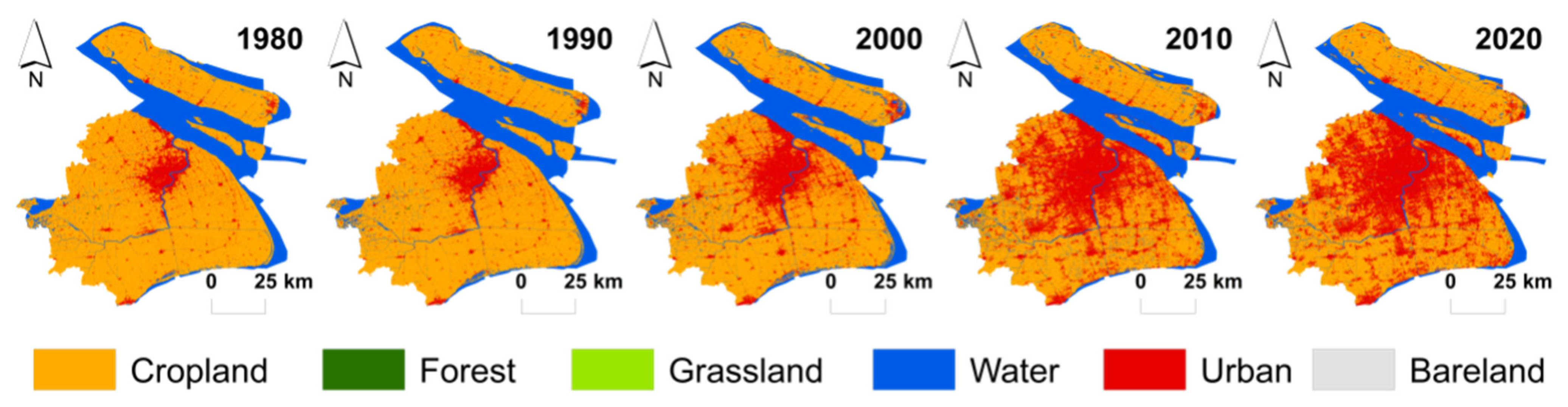
4.1. Classification Maps and Accuracy Assessment

Table 7. The user accuracy (UA), producer accuracy (PA), overall accuracy, and Kappa values of the classification results.

Year	Cropland		Forest		Grassland		Water		Built-up		Bareland		Overall Accuracy	Kappa Coefficient
	UA	PA	UA	PA	UA	PA	UA	PA	UA	PA	UA	PA
1980	0.957	0.988	0.951	0.933	0.882	0.652	0.948	0.964	0.885	0.946	1	0.658	0.938	0.913
1990	0.951	0.993	0.928	0.936	0.889	0.762	0.964	0.89	0.921	0.952	0.921	0.795	0.934	0.907
2000	0.957	0.979	0.888	0.958	0.914	0.796	0.953	0.92	0.924	0.891	0.809	0.809	0.928	0.898
2010	0.942	0.981	0.962	0.962	0.883	0.791	0.978	0.957	0.875	0.927	0.904	0.904	0.933	0.903
2020	0.963	0.989	0.967	0.971	0.963	0.770	0.883	0.988	0.914	0.949	0.94	0.851	0.903	0.926

details the UA, PA, OA, and KC for each year and their class. Statistically, there were higher OA and KC values recorded for the RF classifier. As such, this machine learning classifier has the capacity to reliably elevate the classified maps’s quality, thereby offering a reliable source of data that can facilitate both landscape pattern analysis and spatial mapping.

For the optimal granularity calculation, Figure 4 sets out the landscape metric variations’ response to granularity at the landscape level for each year. As can be seen from the CV results, in 2020, over 5% met the inflection point of the selected metrics. Figure 5 details landscape metrics’ granularity effect at the landscape level. In this study, the optimum grain size for landscape pattern analysis was 70 m. This is valuable for understanding the change information.

Applying the flow method, Figure 6 illustrates land-use pattern classifications for Shanghai for the years 1980 to 2020, whilst Figure 7 displays the open and non-open space patterns over the same period.

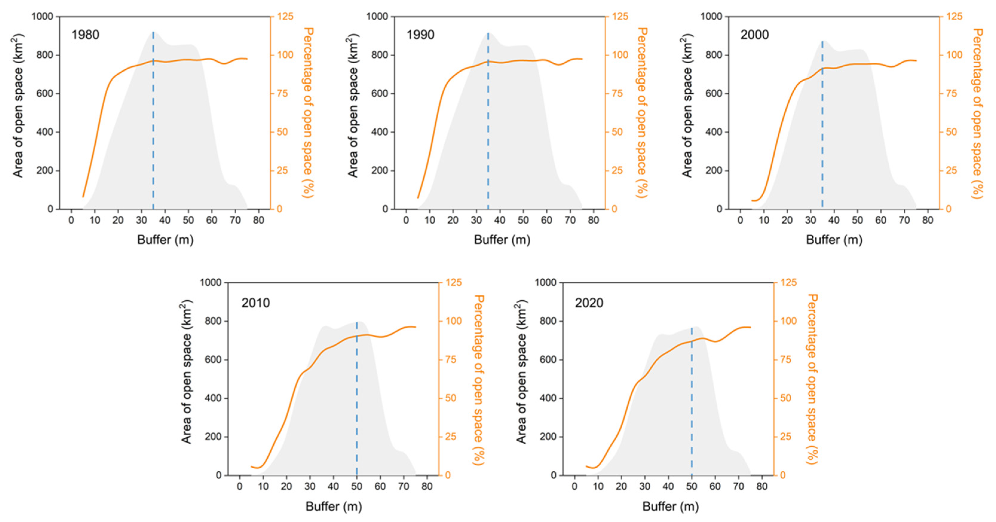
4.2. Spatio-Temporal Trends Present in the Open Space Analysis

4.2.1. Composition Changes in Open Space

(1)

Open space ratio changes between 1980 and 2020

As shown in

Table 8. The overall changes in urban open space (UOS) of Shanghai in 1980–2020.

Land-Use Type		1980	1990	2000	2010	2020
OS1: Cropland	Area (km2)	5719.2912	5590.098	5076.6678	4344.2685	4181.7807
	Percent (%)	70.97	69.3669	62.9958	53.907	51.89
OS2: Forest	Area (km2)	3.7485	3.7206	7.4781	12.9294	10.0332
	Percent (%)	0.0465	0.04616	0.09279	0.160439	0.1245
OS3: Grassland	Area (km²)	0.1638	0.1422	0.0405	3.3246	0.0891
	Percent (%)	0.00203	0.001764	0.00050256	0.04125	0.00110
OS4: Water	Area (km2)	1676.9322	1728.2043	1663.8174	1570.4055	1419.0417
	Percent (%)	20.8088	21.4451	20.646	19.487002	17.6087
Total open space	Area (km2)	7400.1357	7322.1651	6748.0038	5930.928	5610.9447
	Percent (%)	91.827	90.86	83.73529	73.59628	69.625
NOS1: Built-up	Area (km2)	657.3636	735.5268	1310.6466	2127.5253	2447.5698
	Percent (%)	8.157	9.127	16.2636	26.4002	30.3716
NOS2: Bareland	Area (km2)	1.2339	1.0413	0.0828	0.2799	0.2187
	Percent (%)	0.0153	0.01292	0.00102746	0.00347	0.0027
Total: Non-open space	Area (km2)	658.5975	736.5681	1310.7294	2127.8052	2447.7885
	Percent (%)	8.173	9.14	16.2647	26.4037	30.3743

, the area of open space in Shanghai steadily decreased from 1980 to 2020; over this same period, the area of non-open space increased. Specifically, the proportion of open space declined from 91.83% in 1980 to 69.23% in 2020; by way of contrast, the size of the built-up area jumped from 8.16% to 30.37% over the same period. Of the various open space types, cropland experienced the most significant decrease, whilst the proportions of waterbody, forest, and grassland remained relatively stable. To be precise, cropland substantially reduced, falling from 70.97% to 51.89%; even so, it still accounted for the largest open land type in Shanghai. Hence, the loss of open space in the city is largely related to the decrease in cropland. Meanwhile, forest remained relatively stable at 0.1%, whilst grassland initially decreased before then beginning to increase again after 2000, peaking in 2010. Finally, although the area of water bodies remained relatively stable, it nevertheless continuously decreased between 1980 to 2020. As the city grew in size due to its increasing population and growing commercial activities and infrastructure improvements, the built-up area expanded to 2447.5698 km² by 2020, whilst open space increased to 5610.9447 km². The full figures are set out in Table 8.

(2)

Open space changes: a directional perspective

From Figure 8, overall land use in the study area over the study period was evenly distributed in eight directions. However, the distributions of open space subtypes in these eight directions were dissimilar. In general, the total amount of open space decreased over time in every direction. However, it should be noted that the changes in the four open space types differed significantly across all directions. The proportion of open space was largely the same for all directions, indicating that UOS is evenly districted across Shanghai, which may be attributable to the cropland. The distribution of and changes in cropland were not dissimilar to the overall open space, in that there was a dramatic loss of cropland in all directions. Contrastingly, the built-up area substantially expanded in all directions, suggesting that the encroachment on suburban cropland was driving urbanization in the city.

Cropland gradually decreased in all directions, most likely due to the “Grain for Green” program, intimated by the government to mitigate and prevent flooding and soil erosion. Meanwhile, there was a change in forested areas in all directions, though this change was most concentrated in the southwest (Sheshan National Forest Park), the southeast (Fengxian Forest Park), and north (Chongming Island’s DongPing National Forest Park). The timing of this change likely aligns with the point when ecological policy began to be developed.

Grassland increased up to 2010 before returning to its starting point, most obviously in the southwest in 2010. Moreover, as the Yangtze River runs through Shanghai in the north and the city is bordered by the sea to the east, water bodies are mainly located in these directions. Though these waterbodies remained stable, there was a significant decrease in water bodies in the southeast and east, which may be attributable to the land reclamation of tidal flats (i.e., the conversion of sea area into useable land). Elsewhere, the decrease in the water bodies in the north and northeast was largely due to sediment deposition, which is reflected in the inland expansion of Chongming Island.

The built-up area also increased in all directions, though most notably in the southeast (Song Jiang), where Songjiang New City has been selected for development as an important new Shanghai satellite city. Interestingly, as the government implemented real estate management measures in this area, it determined the speed of urbanization. Finally, unused land (Barehand) gradually decreased in all directions, though this was negligible and significantly influenced the proportion of non-open space.

(3)

Open space changes along the concentric buffers

The majority of Shanghai falls within Buffer 15, where the open space area changed significantly (Figure 9). From a time-dimension perspective, the open space ratio of each buffer decreased at a fast pace, moving from the city center in an outward direction to the suburbs. This was most clear between Buffers 2 and 7, after which point the change largely stabilized. Outside of Buffer 8, there are many satellite towns and new towns located outside of the Suburban Ring Expressway. The open space area in Buffer 1 remained largely unchanged over the study period. Moreover, the trends relating to the maximum open space area corresponding to the buffer area changed between the interval’s years. For instance, in 1980, 1990, and 2000, the largest open space area was in Buffer 7, whilst in 2010 and 2020, this was in Buffer 10. Thus, it can be concluded that open spaces are both declining and moving away from the city center.

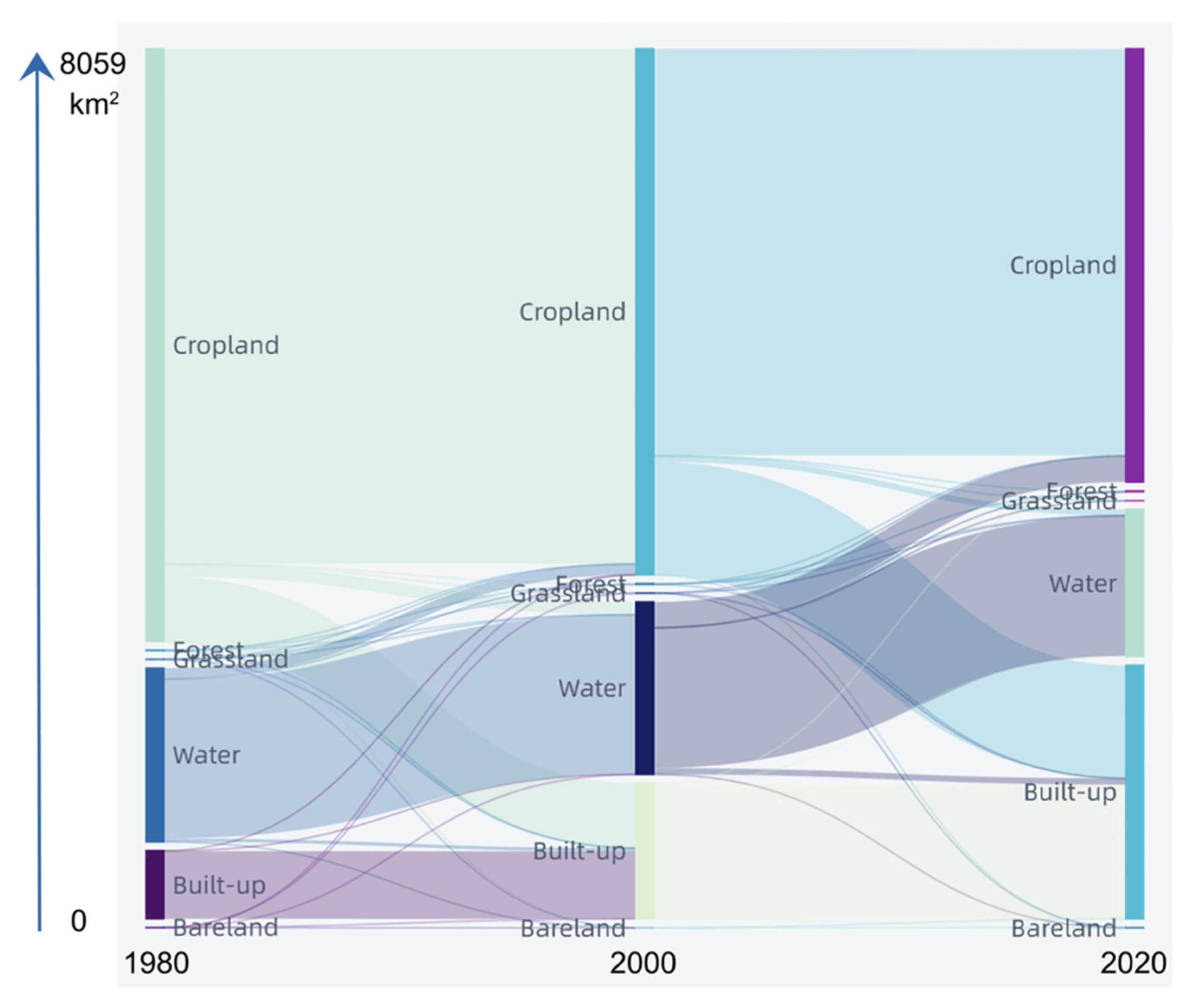
4.2.2. Open Space Change Transitions

The transition matrix is key to analyzing the temporal changes within LULC categories. Specifically, the matrix reflects the proportions of pixels that changed from one land-use category to another. As noted above, the transfer matrixes of land-cover types for the 1980–2000 and 2000–2020 periods were calculated and constructed using ArcGIS10.4 and Excel (

Table 9. Transition matrix of land use in Shanghai from 1980 to 2020 (km²).

Periods	Land-Use Types	Cropland	Forest	Grassland	Water	Built-Up	Bareland
1980–2000	Cropland	4969.49	3.99	0.03	121.08	624.71	0.00
	Forest	1.21	2.44	0.00	0.03	0.07	0.00
	Grassland	0.00	0.00	0.01	0.01	0.14	0.00
	Water	105.12	1.05	0.00	1538.74	32.00	0.03
	Built-up	0.85	0.00	0.00	3.93	652.58	0.00
	Bareland	0.00	0.00	0.01	0.03	1.14	0.05
2000–2020	Cropland	3922.93	6.75	0.08	57.10	1089.68	0.12
	Forest	4.41	2.61	0.00	0.16	0.29	0.00
	Grassland	0.00	0.00	0.00	0.00	0.04	0.00
	Water	249.00	0.67	0.01	1354.78	59.28	0.09
	Built-up	5.45	0.00	0.00	7.00	1298.20	0.00
	Bareland	0.00	0.00	0.00	0.00	0.07	0.01

). Shanghai’s overall transfer trend during the study period can be understood by referencing the land-cover transfer matrix. From 1980 to 2000, the transfer changes between different land-cover types were more significant than in the rest of the study period. As a result, changes in cropland, water, and built-up area were more noticeable; to be precise, 624.71 km² of cropland was converted into built-up areas. The second largest transfer was from cropland to water (105.12 km²). A similar situation occurred in the 2000–2020 period, which was characterized by the conversion of cropland into built-up areas (1089.687 km²). A review of the net gains and losses during the period (Figure 10) shows that cropland experienced the greatest loss, whilst there was a simultaneous increase in the built-up area.

4.2.3. Landscape Metrics Analysis

A synoptic analysis of the landscape metrics summarizes the landscape’s configuration and composition. Shanghai’s various landscape indices cumulatively reflect the temporal and spatial evolution of the city’s open spaces whilst also providing information on the relationship between landscape patterns and landscape change processes. The classification results for the study period were converted into GRID format to calculate the landscape metrics in FRAGSTATS 4.2 [64] (

Table 10. Synoptic open space landscape metrics analysis from 1980 to 2020.

Year	ED	TA	PAFRAC	AI	COHESION	CONTAG	LSI	NP	PD	PLADJ	SPLIT	DIVISION	PRD	SHDI	SHEI
1980	23.93	10.74	2.94	95.52	97.14	32.92	1.18	2.05	18.80	86.09	1.11	0.08	13.59	0.13	0.18
1990	24.19	10.74	1.61	95.53	97.20	32.74	1.19	2.04	18.75	86.05	1.12	0.08	13.63	0.13	0.19
2000	31.45	10.74	3.51	94.61	96.64	32.78	1.25	2.25	20.63	84.96	1.20	0.12	14.15	0.18	0.26
2010	41.92	10.74	9.43	93.18	96.03	32.48	1.33	2.60	23.90	83.39	1.29	0.17	14.77	0.24	0.34
2020	44.24	10.74	8.48	92.91	95.86	32.97	1.35	2.68	24.57	83.04	1.32	0.18	14.99	0.25	0.37

). Adopting a broad view, the PD (fragmentation degree) and ED (fragmentation degree) charted a general upward trend. These change trends increased over the 40-year study period, both of which indicate the fluctuating patch fragmentation. Additionally, AI continuously followed a continuously decreasing trend between 1980 and 2020, reflecting the decomposition process. Furthermore, the SHDI and SHEI values gradually increased, suggesting that the proportion of the differences between landscape types became more significant, whilst the distribution became more uneven and landscape heterogeneity increased.

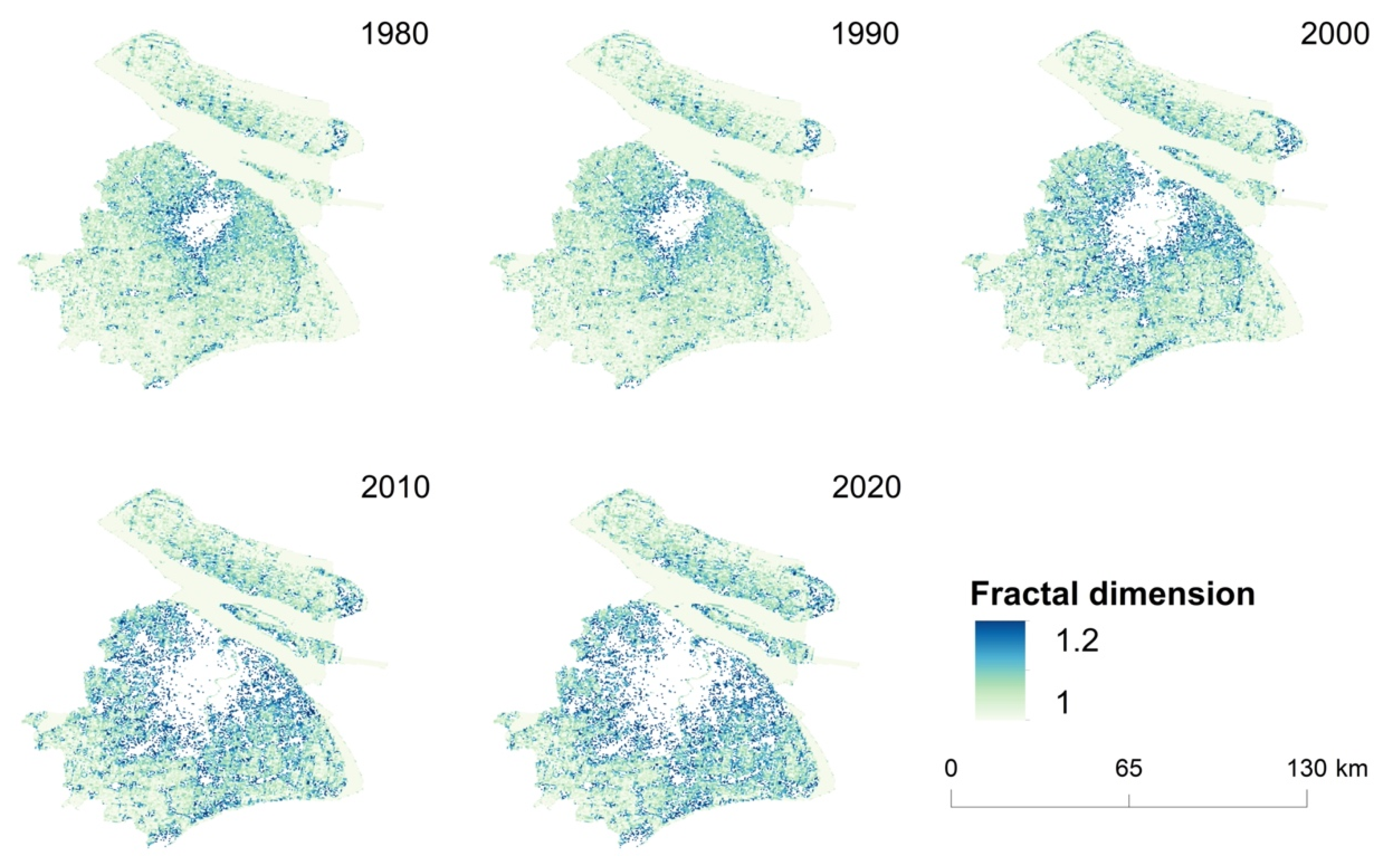
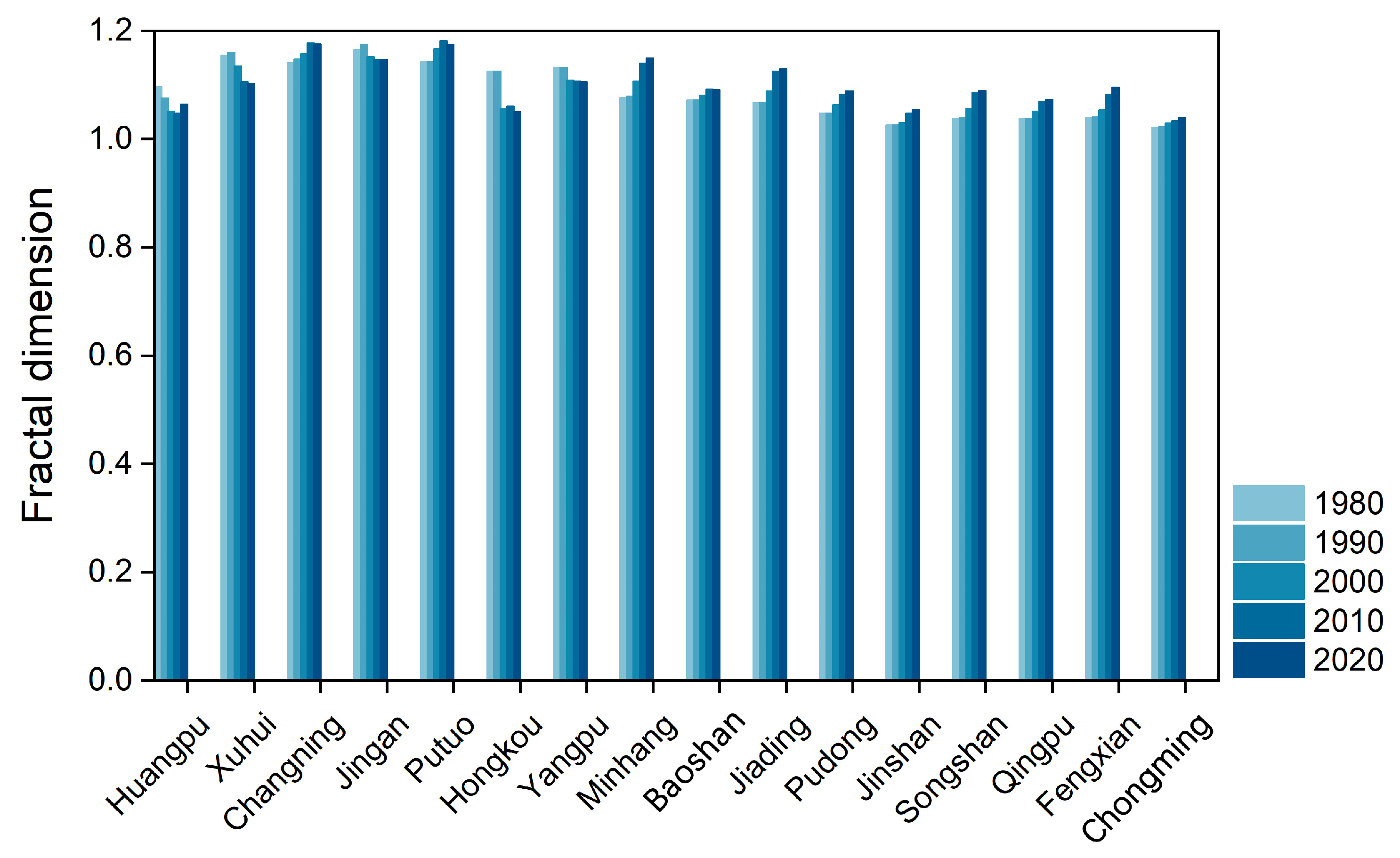
4.2.4. Fractal Dimension

The grid dimension embodies the spatial distribution of UOSs and the balance between them. By analyzing the D values for the entire study area, the D values can be seen to convey the complexity of open space, with fractal dimensions lying between 2.04 and 2.23 (

Table 11. The metrics of open space in study area at five times phase. “P” and “A” represent perimeter and areas of patches, respectively; “D” represents Fractal dimension.

Year	P (m)	A (m2)	D
1980	27,303.90	5723.20	2.04
1990	28,324.92	5593.96	2.05
2000	35,013.42	5084.19	2.13
2010	43,279.32	4360.52	2.22
2020	43,110.24	4191.90	2.23

). The maximum fractal dimension was 2.04 (1980), whilst the minimum was 2.23 (2020). In general, the fractal dimension of open space increases year on year; as a result, the element shape is complex and features an irregular boundary that changes over time. As urban construction and the influence of human activities have grown over time, Shanghai’s open space spatial pattern has gradually become fractured and irregular, forming a complex geometry.

The fractal dimension change trends of the 16 districts are shown in Figure 11 and Figure 12. Among these districts, the fractal dimensions of the open space areas in the city center (Huangpu, Xuhui, Jing’an, Hongkou, and Yangpu) decreased each year, forming a fractal shape. This indicates that their evolution was relatively stable, exhibiting a low degree of separation without any significant changes. Contrastingly, Changning and Putuo increased, giving rise to low self-organization and fragmentation. In the sprawl districts, the fractal dimension of open space increased year on year, hinting at the hugely uneven internal distribution of open space. Meanwhile, in Chongming Island, the trend of the scatter fitting line of open space essentially remained stable throughout the study period.

4.2.5. Shanghai NDVI

The NDVIs were selected for the internal years to assess the change characteristics over time. As can be gathered from Figure 13, the NDVI changes in the city indicate there was a decrease (1980–2000) followed by an increase (2010–2020). Notably, this increase was especially marked in each area, especially in the city center. Meanwhile, the vegetation coverage in the suburbs declined from 1980 to 2015, most obviously in the eastern coastal parts of the Pudong district. Meanwhile, due to land reclamation projects seizing water and wetlands for urban development under government planning and management, after 2000 the southeastern part of Pudong experienced the most dramatic changes. For the islands, the NDVI fell from 1980 to 2000 as vegetation coverage reached its nadir in 2000. However, on a more positive note, the vegetation cover in Chongming Island’s southeast region did experience some growth due to coastal land reclamation efforts.

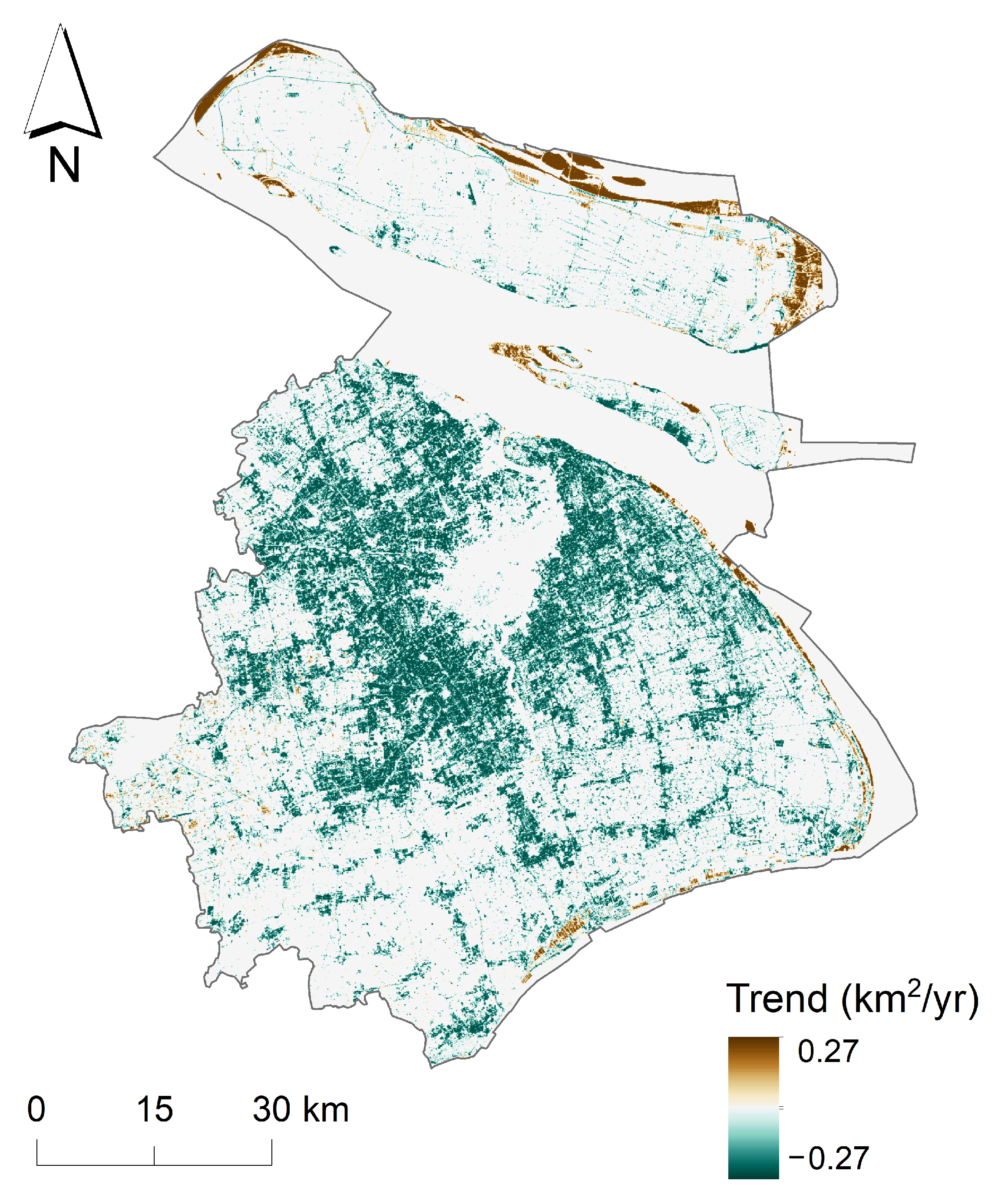
4.2.6. Theil–Sen Median Trend Analysis

At the regional scale, urban open green spaces are generally more scattered and fragmented when they are close to built-up areas due to the greater presence of residential and attached open green space (Figure 14). At the pixel scale, these districts have exhibited significant disparities over the 40-year study period. During this time, in the city center, there was neither a significant increase nor a significant decrease, though open space progressively decreased in urban sprawl areas. As shown in Figure 15, the data on the net gains and losses during the period indicate that Chongming district saw the largest increase, whilst Minhang district saw the largest loss. Though all of the zones saw some change, the most striking were in Minhang, Baoshan, and Jiading.

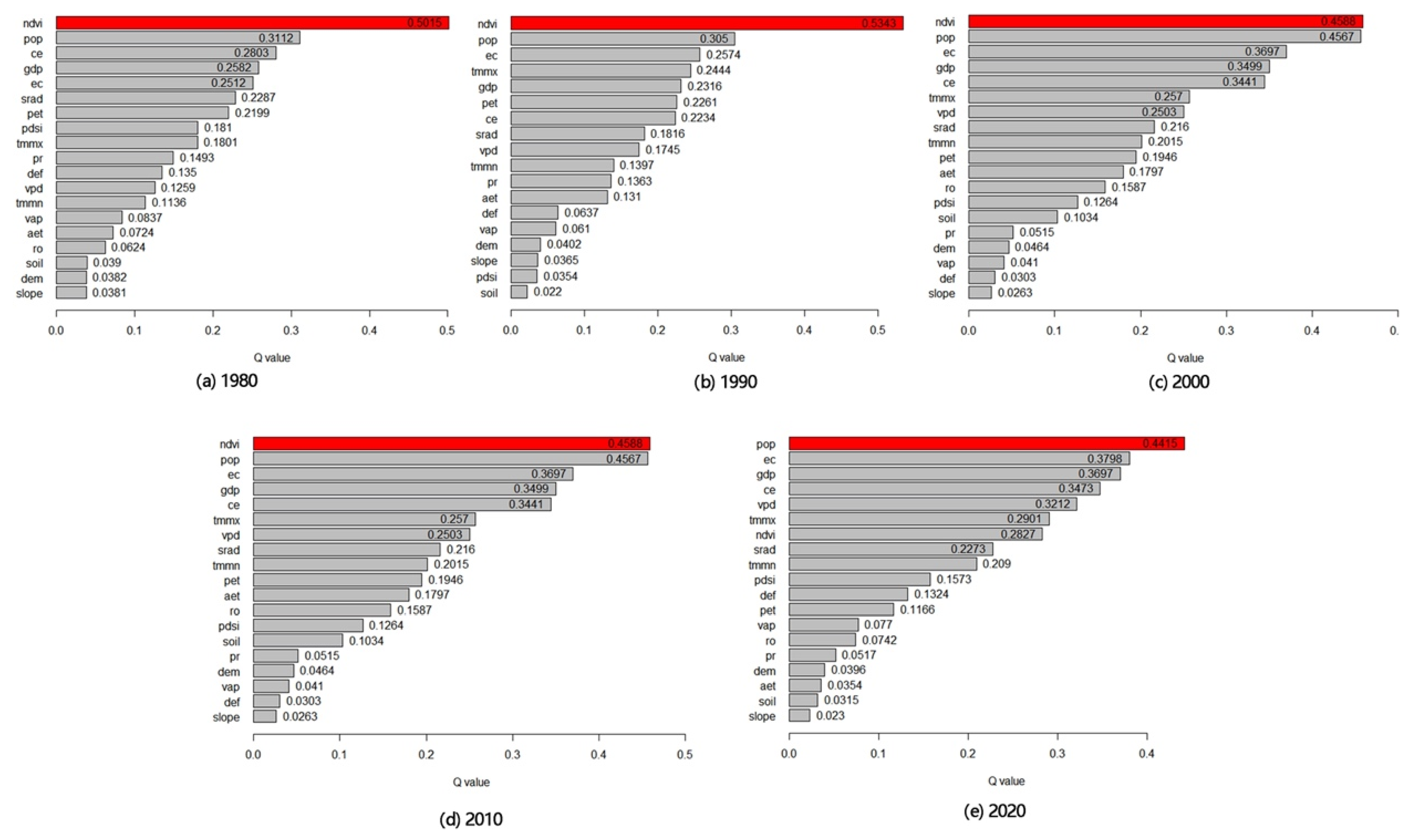
4.3. Analysis of Driving Factors

According to the actual situation of the study area, the natural geographic factors, socioeconomic factors, and climatic factors were divided by using the Jenks natural breaks method [71]. GeoDetector detects and expresses the q value, which represents the relative importance of each explanatory variable (Figure 16). Although the comparison of q-values in the five years shows that separate factors changed uniquely, the values of natural factors (NDVI) and socioeconomic factors (population density, GDP, and electricity consumption) are higher than other indicators as a whole. In 1980, the explanatory power of each index is as follows (top five): NDVI (0.5015) > population density (0.3112) > carbon emission density (0.2803) > GDP (0.2582) > electricity consumption (0.2512). The result shows that the slope, DEM, soil moisture, runoff, and actual evapotranspiration had the weakest correlations with open space changes. In 1990, the driving factors (top five) were ranked in the order of intensity depending on the q-value: NDVI (0.5343) > population density (0.305) > electricity consumption (0.2574) > maximum temperature (0.2444) > GDP (0.2316). The least relevant factors were namely soil moisture, Palmer drought severity index, slope, DEM, and atmospheric pressure. In 2000, the q values of the top five factors were namely NDVI (0.4588) > population density (0.4567) > electricity consumption (0.3697) > GDP (0.3499) > carbon emission density (0.3441). Slope, climate water deficit, atmospheric pressure, DEM, and precipitation had the weakest correlation with open space changes. In 2010, the explanatory power of each index was as follows in the top five: NDVI (0.4588) > population density (0.4567) > electricity consumption (0.3697) > GDP (0.3499) > carbon emission density (0.3441). The least relevant factors were namely slope, climate water deficit, VAP, DEM, and precipitation. By 2020, the top five driving factors were ranked in the order of intensity depending on their q-value: population density (0.4415) > electricity consumption (0.3798) > GDP (0.3697) > carbon emission density (0.3473) > vapor pressure difference (0.3212). Slope, soil moisture, actual evapotranspiration, DEM, and precipitation had the weakest correlation with open space changes.

In addition, in 1980 and 1990 the q-values of the factors were small. By 2000, the explanatory power had increased. In 2000, the explanatory power of population density continued to grow, while the explanatory power of the NDVI decreased. By 2020, overall, the regularity of the explanatory power of various factors on the distribution of UOS was poor, indicating that urban development was a complicated process. Three decades ago, the results show that the NDVI had the greatest correlation with open space change, which may be because higher numbers in the NDVI indicate more green vegetation. However, the q-value of the NDVI showed a decreasing trend in 2020. This might be due to the fact that urban expansion has led to a reduction in natural or semi-natural vegetation surrounding the city center and the suburbs.

By 2020, the population density also had a very high impact on open space changes; furthermore, population growth puts pressure on urban infrastructure, and open spaces are sacrificed to make way for buildings and other infrastructure [72]. This has also been confirmed in Hong Kong [73] and Islamic Mahaud [74]. Population density is the most important factor of the socioeconomic factors, and it is also the driving force for most of the dynamic urban open space change. Population increase directly or indirectly causes urbanization. The growing urban population has resulted in a higher demand for residential space, leading to an expansion of urban development areas and a shift in land-cover categorization.

The correlations between DEM and slope with open space change was smaller because the vast majority of Shanghai’s land area is flat. However, flat terrain is favorable for the development of construction land and plays a beneficial role in promoting the development of construction land in Shanghai. Although natural geographical factors were not an important factor, they cannot be overlooked. The topography and geomorphology of the region have a direct impact on the alteration of open space and spatial structure, exert an effect on the function and structure inside the city, and define the future development trajectory of the city and the spatial arrangement of land use.

Over the five different years, the values of climatic factors have played a certain role in open space changes. Climate change is exacerbating the intensity and frequency of heatwaves, droughts, precipitation, and storms. These severe weather phenomena have a direct influence on urban areas, causing changes in vegetation and the availability of open areas. The escalation of sea levels and coastal erosion will jeopardize the preservation of current parks and open areas located in close proximity to the ocean. For instance, climate change impacts agricultural yields, resulting in alterations to land-use patterns. Climate change has a negative effect on both the deterioration of land and its utilization. Likewise, it plays a crucial role in causing land degradation processes, leading to alterations in open spaces. Shanghai’s wet and dry soil conditions affect the climate and result in the alteration of land use. Likewise, elevated temperatures and increased precipitation will result in winters that are warmer and shorter, leading to alterations in land-use patterns in several locations.

5. Discussion

5.1. An Integrated Approach Describing the Spatiotemporal Dynamics of UOS

Given its crucial role in urban areas, there is great value in better understanding the pattern and trajectory of UOS to inform urban planning. On this basis, this research charts the temporal and spatial evolution of Shanghai’s open space. More specifically, it has confirmed the findings reported in the existing literature on the value of concentric and directional open space ratio analysis when characterizing the spatiotemporal variations in UOS. Thanks to this approach, it was found that the UOS of Shanghai mainly decreased in the east–west direction, changing along the urban–rural gradient. The directional analysis showed that the built-up area substantially and simultaneously increased in the east–west direction. Meanwhile, the concentric analysis results indicate that the expressway functioned as a boundary, restricting urban development and producing different UOS characteristics. It was also found that the classic concentric zone urban development theory could be applied to Shanghai’s land-use pattern during the study period [75], namely in that UOS increased as proximity from the city center increased. After classifying the remote sensing images, it was found that many croplands were converted to built-up areas during the study period, which is reflective of the dramatic change in land use in Shanghai.

The reality of the situation is that open green space in Shanghai has been used to attend to urbanization, industrialization, and their growing demand, which are themselves driven by population growth. Moreover, open spaces in the city center are fragmented, aggregated in the nearest suburban areas, and more scattered in the suburbs. The NDVI reflects a significant disparity in the development of green space and built-up areas during this period of rapid urbanization (though the vegetation index has showed an upward trend in more recent years). The conceptual basis of the NDVI technique is that healthy vegetation is a poor reflector of visible electromagnetic waves due to the presence of chlorophyll. However, the NDVI results may be a result of the streets being narrow in the city center, where the building and the population density are high. Moreover, the increasing density of the city is producing a “Heat Island effect”, increasing temperatures relative to nearby rural areas. In this environment, impervious urban surfaces absorb more sunlight than the surrounding vegetation, resulting in a higher index in the city than the suburbs, even though vegetation cover is lower. Adopting a wider spatial perspective, urban open green spaces tended to become more scattered over the study period, whilst the fractal characteristics showed that the open space patterns were more compacted in the city center than in the nearest suburban areas. The results presented here will be of use in future regional and global land-cover mapping research and confirm the validity of the approach detailed above in carrying out such work.

5.2. Understanding the Driving Policies on Urban Open Spaces Dynamics

As mentioned above, urban open space will be driven by natural geographic, socioeconomic, and climate factors to a certain extent, while policies such as land use and urban construction also directly determine urban open green planning and guide its layout. Thus, this section sorts out the policies that affect its change from a city to sub area (Figure 17).

Shanghai’s municipal government has set out many policies since the 1980s that have significantly shaped the city’s green space [9]. The concepts of “green city”, “ecological city”, “forest city”, and “park city” have steadily emerged over the study period, all of which are geared towards creating a more livable environment in which the city’s residents live in harmony with nature. Regarding the land space planning system, urban green space planning is now designated as special planning, which reflects the elevated status of urban green space in the urban system and the urgent need for high-quality urban development [76,77]. For instance, between 1986 and 1998, Shanghai built a green belt outside of the city center, the Lujiazui Center Green Space, Huangpu riverside promenade, and several recreational parks. In 1994, Shanghai has proposed a “Central City Public Green Spaces Plan” and formed a “Ring, Wedge, Gallery, Garden” spatial pattern. Moreover, the Shanghai government has set out its ambition to build a world-leading eco-island in Chongming in 2016 (Shanghai Municipal Government (SMG, 2016a, 2016b)), creating an ecologically sustainable environment that effectively balances resource utilization and high human standards of living. This policy reflects the trend towards increasing the open space seen in Chongming Island over the study period, where the area of open space has also increased (Figure 8).

More recently, the national Chinese government has exerted its control over the land supply to encourage urban open green space [78], most notably by prioritizing eco-city development. In lockstep, the Shanghai municipal government has implemented policies and measures to strike a balance between competing demands for urbanization development and open green spaces. From the planning documents issued by the Shanghai government, it can be concluded that the city’s greening policies encompass multiple categories and levels (i.e., UGS plans, urban master plans, urban zoning plans, urban biodiversity plans, land-use plans, and urban forest plans) (Figure 17). These policies have all contributed to the observed changes in Shanghai’s open green spaces. There is no denying that the city’s urban open green evolution became more stable once green policies were put in place, demonstrating that the two are inextricably linked.

5.3. Optimizing Strategy

Assessing the spatiotemporal changes in open space yields crucial data that can be applied for landscape planning and urban planning purposes, both of which are vital in sustainably developing and managing Shanghai. Particular attention should be paid to exploring those areas where open green space has decreased or charted a downward trend over the last four decades. The characteristics of open space in Shanghai and the trends it has followed as it has changed over the study period are of great use in achieving sustainable land use in the city moving forward.

To do so, first, the existing open space must be maintained or increased by reducing farmland loss. Additionally, the inefficient use of construction land to meet urbanization demand must be curtailed to curb demand for farmland. Meanwhile, the creation of more forest parks increases the connectivity between residents and the forest. Second, tidal flat reclamation must be carefully managed to maintain the coastal resources and ensure there is sufficient strategic space for long-term development. In particular, attention must be paid to curtailing the decrease in water bodies and increasing coastal wetland reclamation. Regarding the ecological systems, the coastal shelter belt, wetlands, and aquatic plants should be targeted and safeguarded as a means to improve the environmental quality of coastal areas.

6. Conclusions

To plan for the future of urban areas, there is a developing interest in comprehending the spatial pattern and temporal dynamics of open space, which have a significant impact on urban health and quality of life. In this study, we analyze the spatial–temporal changes and identify driving forces for open space changes in Shanghai from 1980 to 2020. Specifically, over forty years, the open space patterns in the city center became increasingly fragmented and decentralized, whilst the open space decreased in size and became more dispersed in the nearest suburban areas. It should also be noted that the NDVI showed an increasing trend between 2000 and 2020. Meanwhile, from the landscape pattern metrics, it is clear that Shanghai’s open space became more fragmented over the study period, producing isolated areas of open space. Its planning has achieved some phased achievements, which are beneficial to assessing the problems and challenges of urban open space scientifically. Furthermore, for the research on driving forces, among the 19 driving factors, NDVI, POP, GDP, and EC contributed more to the change in open space. Our results indicate that both natural geographic, socioeconomic, climatic factors, and policy factors were determined to be the key factors driving the changes in the spatiotemporal dynamics of UOS in the current study. The impacts of socioeconomic factors on the spatial–temporal changes in open space have continually increased over the past 40 years, and were also higher than natural geographic factors to some extent. Additionally, the Random Forest (RF) classifier, which is a robust classification method, was deployed in conjunction with the Google Earth Engine (GEE) platform to analyze images from the years 1980 to 2020. The optimal grain size to produce a high-quality LULC map was calculated to be 70 m. Remote sensing is used in conjunction with data from other sources, which can be integrated as a powerful tool to validate and understand the trend of open space change in cities. The methods employed in this analysis of changing urban open spaces in Shanghai can be applied in other cities to promote more effective and equitable planning of urban spaces. By doing so, this provides a viewpoint for other cities that have experienced similarly rapid expansion. However, due to the lack of detailed documents, it is difficult to provide a quantitative figure for policy factors. Also, the prediction of open space in Shanghai can be researched, so as to promote appropriate designing and improve the utilization rate and sustainable development of urban open space.

References

1. Schell, L.M.; Ulijaszek, S.J.; Schell, L.M.; Ulijaszek, S.J.; McMichael, A.J.; Clark, D.; Huss-Ashmore, R.; Behrman, C.; Diferdinando, G.; Ellison, P.T.; et al. Urbanism, Health and Human Biology in Industrialised Countries; Cambridge University Press: Cambridge, UK, 1999; ISBN 9780521620970. [Google Scholar]
2. Haas, J.; Ban, Y. Urban Growth and Environmental Impacts in Jing-Jin-Ji, the Yangtze, River Delta and the Pearl River Delta. Int. J. Appl. Earth Obs. Geoinf. 2014, 30, 42–55. [Google Scholar] [CrossRef]
3. Kim, K.-H.; Pauleit, S. Landscape Character, Biodiversity and Land Use Planning: The Case of Kwangju City Region, South Korea. Land Use Policy 2007, 24, 264–274. [Google Scholar] [CrossRef]
4. Yuan, F.; Bauer, M.E. Comparison of Impervious Surface Area and Normalized Difference Vegetation Index as Indicators of Surface Urban Heat Island Effects in Landsat Imagery. Remote Sens. Environ. 2007, 106, 375–386. [Google Scholar] [CrossRef]
5. Yeh, C.-T.; Huang, S.-L. Investigating Spatiotemporal Patterns of Landscape Diversity in Response to Urbanization. Landsc. Urban Plan. 2009, 93, 151–162. [Google Scholar] [CrossRef]
6. Davies, R.G.; Barbosa, O.; Fuller, R.A.; Tratalos, J.; Burke, N.; Lewis, D.; Warren, P.H.; Gaston, K.J. City-Wide Relationships between Green Spaces, Urban Land Use and Topography. Urban Ecosyst. 2008, 11, 269–287. [Google Scholar] [CrossRef]
7. Chen, W.Y.; Jim, C.Y. Assessment and Valuation of the Ecosystem Services Provided by Urban Forests. In Ecology, Planning, and Management of Urban Forests: International Perspectives; Carreiro, M.M., Song, Y.-C., Wu, J., Eds.; Springer: New York, NY, USA, 2008; pp. 53–83. ISBN 9780387714257. [Google Scholar]
8. Wang, J.; Li, L.; Zhang, T.; Chen, L.; Wen, M.; Liu, W.; Hu, S. Optimal Grain Size Based Landscape Pattern Analysis for Shanghai Using Landsat Images from 1998 to 2017. Pol. J. Environ. Stud. 2021, 30, 2799–2813. [Google Scholar] [CrossRef] [PubMed]
9. Wu, Z.; Chen, R.; Meadows, M.E.; Sengupta, D.; Xu, D. Changing Urban Green Spaces in Shanghai: Trends, Drivers and Policy Implications. Land Use Policy 2019, 87, 104080. [Google Scholar] [CrossRef]
10. Li, J.; Li, C.; Zhu, F.; Song, C.; Wu, J. Spatiotemporal Pattern of Urbanization in Shanghai, China between 1989 and 2005. Landsc. Ecol. 2013, 28, 1545–1565. [Google Scholar] [CrossRef]
11. Liu, S.; Zhang, X.; Feng, Y.; Xie, H.; Jiang, L.; Lei, Z. Spatiotemporal Dynamics of Urban Green Space Influenced by Rapid Urbanization and Land Use Policies in Shanghai. For. Trees Livelihoods 2021, 12, 476. [Google Scholar] [CrossRef]
12. Amani, M.; Ghorbanian, A.; Ahmadi, S.A.; Kakooei, M.; Moghimi, A.; Mirmazloumi, S.M.; Moghaddam, S.H.A.; Mahdavi, S.; Ghahremanloo, M.; Parsian, S.; et al. Google Earth Engine Cloud Computing Platform for Remote Sensing Big Data Applications: A Comprehensive Review. IEEE J. Sel. Top. Appl. Earth Obs. Remote Sens. 2020, 13, 5326–5350. [Google Scholar] [CrossRef]
13. Uy, P.D.; Nakagoshi, N. Analyzing Urban Green Space Pattern and Eco-Network in Hanoi, Vietnam. Landsc. Ecol. Eng. 2007, 3, 143–157. [Google Scholar] [CrossRef]
14. Xu, H.; Cui, J. Assessing Changes in Green Space of Suzhou City Using Remote-Sensing Images and Landscape Metrics. TC 2016, 620, 45999-83. [Google Scholar]
15. Kong, F.; Nakagoshi, N. Spatial-Temporal Gradient Analysis of Urban Green Spaces in Jinan, China. Landsc. Urban Plan. 2006, 78, 147–164. [Google Scholar] [CrossRef]
16. Liu, J.; Zhang, L.; Zhang, Q.; Li, C.; Zhang, G.; Wang, Y. Spatiotemporal Evolution Differences of Urban Green Space: A Comparative Case Study of Shanghai and Xuchang in China. Land Use Policy 2022, 112, 105824. [Google Scholar] [CrossRef]
17. Xiao, Z.; Tian, Y.; Hao, L. Evolution of Green Space Based on Remote Sensing Images in Zhengdong New District. Proc. Int. Wirel. Commun. Mob. Comput. Conf. 2022, 2022, 3599045. [Google Scholar] [CrossRef]
18. Yang, J.; Zhang, F.; Shi, B. Analysis of Open Space Types in Urban Centers Based on Functional Features. E3S Web Conf. 2019, 79, 01009. [Google Scholar] [CrossRef]
19. Ma, L.; Li, M.; Ma, X.; Cheng, L.; Du, P.; Liu, Y. A Review of Supervised Object-Based Land-Cover Image Classification. ISPRS J. Photogramm. Remote Sens. 2017, 130, 277–293. [Google Scholar] [CrossRef]
20. Kong, F.; Nakagoshi, N. Changes of Urban Green Spaces and Their Driving Forces: A Case Study of Jinan City, China. J. Int. Dev. Coop. 2005, 11, 97–109. [Google Scholar]
21. Tan, P.Y.; Wang, J.; Sia, A. Perspectives on Five Decades of the Urban Greening of Singapore. Cities 2013, 32, 24–32. [Google Scholar] [CrossRef]
22. Zhou, X.; Wang, Y.-C. Spatial–temporal Dynamics of Urban Green Space in Response to Rapid Urbanization and Greening Policies. Landsc. Urban Plan. 2011, 100, 268–277. [Google Scholar] [CrossRef]
23. Shu, B.; Zhang, H.; Li, Y.; Qu, Y.; Chen, L. Spatiotemporal Variation Analysis of Driving Forces of Urban Land Spatial Expansion Using Logistic Regression: A Case Study of Port Towns in Taicang City, China. Habitat Int. 2014, 43, 181–190. [Google Scholar] [CrossRef]
24. Wang, J.; Xu, C. Geodetector: Principle and prospective. Acta Geogr. Sin. 2017, 72, 116–134. [Google Scholar]
25. Yang, H.; Xu, T.; Chen, D.; Yang, H.; Pu, L. Direct Modeling of Subway Ridership at the Station Level: A Study Based on Mixed Geographically Weighted Regression. Can. J. Civ. Eng. 2020, 47, 534–545. [Google Scholar] [CrossRef]
26. Mohamed, A.; Worku, H. Simulating Urban Land Use and Cover Dynamics Using Cellular Automata and Markov Chain Approach in Addis Ababa and the Surrounding. Urban Clim. 2020, 31, 100545. [Google Scholar] [CrossRef]
27. Wu, S.; Wang, D.; Yan, Z.; Wang, X.; Han, J. Spatiotemporal Dynamics of Urban Green Space in Changchun: Changes, Transformations, Landscape Patterns, and Drivers. Ecol. Indic. 2023, 147, 109958. [Google Scholar] [CrossRef]
28. Ouyang, X.; Tang, L.; Wei, X.; Li, Y. Spatial Interaction between Urbanization and Ecosystem Services in Chinese Urban Agglomerations. Land Use Policy 2021, 109, 105587. [Google Scholar] [CrossRef]
29. Liu, C.; Xu, Y.; Lu, X.; Han, J. Trade-Offs and Driving Forces of Land Use Functions in Ecologically Fragile Areas of Northern Hebei Province: Spatiotemporal Analysis. Land Use Policy 2021, 104, 105387. [Google Scholar] [CrossRef]
30. Shanghai Municipal Government (SMG). Shanghai Master Plan 2017–2035. 2018. Available online: http://www.shanghai.gov.cn/newshanghai/xxgkfj/2035004.pdf (accessed on 1 March 2023).
31. Liu, J.; Liu, M.; Tian, H.; Zhuang, D.; Zhang, Z.; Zhang, W.; Tang, X.; Deng, X. Spatial and Temporal Patterns of China’s Cropland during 1990–2000: An Analysis Based on Landsat TM Data. Remote Sens. Environ. 2005, 98, 442–456. [Google Scholar] [CrossRef]
32. Institute of Geographical Sciences and Resources Research, CAS, Resource and Environmental Science and Data Centre. Available online: https://www.resdc.cn (accessed on 27 May 2022).
33. Huang, C.; Xu, N. Climatic Factors Dominate the Spatial Patterns of Urban Green Space Coverage in the Contiguous United States. Int. J. Appl. Earth Obs. Geoinf. 2022, 107, 102691. [Google Scholar] [CrossRef]
34. Dobbs, C.; Nitschke, C.; Kendal, D. Assessing the Drivers Shaping Global Patterns of Urban Vegetation Landscape Structure. Sci. Total Environ. 2017, 592, 171–177. [Google Scholar] [CrossRef] [PubMed]
35. USGS.gov. Science for a Changing World. Available online: https://earthexplorer.usgs.gov/ (accessed on 27 May 2023).
36. Climatologylab. Available online: https://www.climatologylab.org/terraclimate.html (accessed on 27 June 2023).
37. Chen, J.; Gao, M.; Cheng, S.; Hou, W.; Song, M.; Liu, X.; Liu, Y. Global 1 Km × 1 Km Gridded Revised Real Gross Domestic Product and Electricity Consumption during 1992–2019 Based on Calibrated Nighttime Light Data. Sci. Data 2022, 9, 202. [Google Scholar] [CrossRef] [PubMed]
38. Open Spatial Demographic Data and Research. Available online: https://www.worldpop.org/ (accessed on 3 May 2023).
39. Odiac-Fossil fuel CO2 emission data product. Available online: https://odiac.org/index.html (accessed on 27 May 2023).
40. Kumar, L.; Mutanga, O. Google Earth Engine Applications since Inception: Usage, Trends, and Potential. Remote Sens. 2018, 10, 1509. [Google Scholar] [CrossRef]
41. Tamiminia, H.; Salehi, B.; Mahdianpari, M.; Quackenbush, L.; Adeli, S.; Brisco, B. Google Earth Engine for Geo-Big Data Applications: A Meta-Analysis and Systematic Review. ISPRS J. Photogramm Remote Sens. 2020, 164, 152–170. [Google Scholar] [CrossRef]
42. Belgiu, M.; Drăguţ, L. Random Forest in Remote Sensing: A Review of Applications and Future Directions. ISPRS J. Photogramm Remote Sens. 2016, 114, 24–31. [Google Scholar] [CrossRef]
43. Breiman, L. Random Forests. Mach. Learn. 2001, 45, 5–32. [Google Scholar] [CrossRef]
44. Rabiei-Dastjerdi, H.; Amini, S.; McArdle, G.; Homayouni, S. City-Region or City? That Is the Question: Modelling Sprawl in Isfahan Using Geospatial Data and Technology. GeoJournal 2022, 88 (Suppl. S1), 135–155. [Google Scholar] [CrossRef]
45. Hansen, M.C.; Roy, D.P.; Lindquist, E.; Adusei, B.; Justice, C.O.; Altstatt, A. A Method for Integrating MODIS and Landsat Data for Systematic Monitoring of Forest Cover and Change in the Congo Basin. Remote Sens. Environ. 2008, 112, 2495–2513. [Google Scholar] [CrossRef]
46. Pettorelli, N.; Vik, J.O.; Mysterud, A.; Gaillard, J.-M.; Tucker, C.J.; Stenseth, N.C. Using the Satellite-Derived NDVI to Assess Ecological Responses to Environmental Change. Trends Ecol. Evol. 2005, 20, 503–510. [Google Scholar] [CrossRef] [PubMed]
47. Gao, B.-C. NDWI—A Normalized Difference Water Index for Remote Sensing of Vegetation Liquid Water from Space. Remote Sens. Environ. 1996, 58, 257–266. [Google Scholar] [CrossRef]
48. Zha, Y.; Gao, J.; Ni, S. Use of Normalized Difference Built-up Index in Automatically Mapping Urban Areas from TM Imagery. Int. J. Remote Sens. 2003, 24, 583–594. [Google Scholar] [CrossRef]
49. Xu, H. Modification of Normalised Difference Water Index (NDWI) to Enhance Open Water Features in Remotely Sensed Imagery. Int. J. Remote Sens. 2006, 27, 3025–3033. [Google Scholar] [CrossRef]
50. Rennó, C.D.; Nobre, A.D.; Cuartas, L.A.; Soares, J.V.; Hodnett, M.G.; Tomasella, J.; Waterloo, M.J. HAND, a New Terrain Descriptor Using SRTM-DEM: Mapping Terra-Firme Rainforest Environments in Amazonia. Remote Sens. Environ. 2008, 112, 3469–3481. [Google Scholar] [CrossRef]
51. Wang, Z.; Bai, T.; Xu, D.; Kang, J.; Shi, J.; Fang, H.; Nie, C.; Zhang, Z.; Yan, P.; Wang, D. Temporal and Spatial Changes in Vegetation Ecological Quality and Driving Mechanism in Kökyar Project Area from 2000 to 2021. Sustainability 2022, 14, 7668. [Google Scholar] [CrossRef]
52. Behera, M.D.; Borate, S.N.; Panda, S.N.; Behera, P.R.; Roy, P.S. Modelling and Analyzing the Watershed Dynamics Using Cellular Automata (CA)–Markov Model—A Geo-Information Based Approach. J. Earth Syst. Sci. 2012, 121, 1011–1024. [Google Scholar] [CrossRef]
53. Halmy, M.W.A.; Gessler, P.E.; Hicke, J.A.; Salem, B.B. Land Use/land Cover Change Detection and Prediction in the North-Western Coastal Desert of Egypt Using Markov-CA. Appl. Geogr. 2015, 63, 101–112. [Google Scholar] [CrossRef]
54. Pontius, R.G.; Millones, M. Death to Kappa: Birth of Quantity Disagreement and Allocation Disagreement for Accuracy Assessment. Int. J. Remote Sens. 2011, 32, 4407–4429. [Google Scholar] [CrossRef]
55. Wu, J. Effects of Changing Scale on Landscape Pattern Analysis: Scaling Relations. Landsc. Ecol. 2004, 19, 125–138. [Google Scholar] [CrossRef]
56. Buyantuyev, A.; Wu, J.; Gries, C. Multiscale Analysis of the Urbanization Pattern of the Phoenix Metropolitan Landscape of USA: Time, Space and Thematic Resolution. Landsc. Urban Plan. 2010, 94, 206–217. [Google Scholar] [CrossRef]
57. Fang, S.; Zhao, Y.; Han, L.; Ma, C. Analysis of Landscape Patterns of Arid Valleys in China, Based on Grain Size Effect. Sustain. Sci. Pract. Policy 2017, 9, 2263. [Google Scholar] [CrossRef]
58. Teng, M.; Zeng, L.; Zhou, Z.; Wang, P.; Xiao, W.; Dian, Y. Responses of Landscape Metrics to Altering Grain Size in the Three Gorges Reservoir Landscape in China. Environ. Earth Sci. 2016, 75, 1055. [Google Scholar] [CrossRef]
59. Yin, J.; Yin, Z.; Zhong, H.; Xu, S.; Hu, X.; Wang, J.; Wu, J. Monitoring Urban Expansion and Land Use/land Cover Changes of Shanghai Metropolitan Area during the Transitional Economy (1979–2009) in China. Environ. Monit. Assess. 2011, 177, 609–621. [Google Scholar] [CrossRef] [PubMed]
60. Xu, J.; Liao, B.; Shen, Q.; Zhang, F.; Mei, A. Urban Spatial Restructuring in Transitional economy—Changing Land Use Pattern in Shanghai. Chin. Geogr. Sci. 2007, 17, 19–27. [Google Scholar] [CrossRef]
61. Yu, Z.; Wang, Y.; Deng, J.; Shen, Z.; Wang, K.; Zhu, J.; Gan, M. Dynamics of Hierarchical Urban Green Space Patches and Implications for Management Policy. Sensors 2017, 17. [Google Scholar] [CrossRef] [PubMed]
62. Biondini, M.; Kandus, P. Transition Matrix Analysis of Land-Cover Change in the Accretion Area of the Lower Delta of the Paraná River (Argentina) Reveals Two Succession Pathways. Wetlands 2006, 26, 981–991. [Google Scholar] [CrossRef]
63. Feng, Y.; Liu, Y.; Tong, X. Spatiotemporal Variation of Landscape Patterns and Their Spatial Determinants in Shanghai, China. Ecol. Indic. 2018, 87, 22–32. [Google Scholar] [CrossRef]
64. McGarigal, K.; Marks, B.J. FRAGSTATS: Spatial Pattern Analysis Program for Quantifying Landscape Structure; U.S. Department of Agriculture, Forest Service, Pacific Northwest Research Station: Portland, OR, USA, 1995.
65. Lamine, S.; Petropoulos, G.P.; Singh, S.K.; Szabó, S.; Bachari, N.E.I.; Srivastava, P.K.; Suman, S. Quantifying Land Use/land Cover Spatio-Temporal Landscape Pattern Dynamics from Hyperion Using SVMs Classifier and FRAGSTATS®. Geocarto Int. 2018, 33, 862–878. [Google Scholar] [CrossRef]
66. Versini, P.-A.; Gires, A.; Tchiguirinskaia, I.; Schertzer, D. Fractal Analysis of Green Roof Spatial Implementation in European Cities. Urban For. Urban Greening 2020, 49, 126629. [Google Scholar] [CrossRef]
67. Aburas, M.M.; Abdullah, S.H.; Ramli, M.F.; Ash’aari, Z.H. Measuring Land Cover Change in Seremban, Malaysia Using NDVI Index. Procedia Environ. Sci. 2015, 30, 238–243. [Google Scholar] [CrossRef]
68. Rouse, J.W., Jr.; Haas, R.H.; Schell, J.A.; Deering, D.W. Monitoring Vegetation Systems in the Great Plains with Erts. In NASA Special Publication; NASA, Goddard Space Flight Center 3d: Washington, DC, USA, 1974; Volume 351, p. 309. [Google Scholar]
69. Burn, D.H.; Hag Elnur, M.A. Detection of Hydrologic Trends and Variability. J. Hydrol. 2002, 255, 107–122. [Google Scholar] [CrossRef]
70. Wang, J.; Li, X.; Christakos, G.; Liao, Y.; Zhang, T.; Gu, X.; Zheng, X. Geographical Detectors-Based Health Risk Assessment and Its Application in the Neural Tube Defects Study of the Heshun Region, China. Int. J. Geogr. Inf. Sci. 2010, 24, 107–127. [Google Scholar] [CrossRef]
71. Jenks, G.F. The Data Model Concept in Statistical Mapping. Int. Yearb. Cartogr. 1967, 7, 186–190. [Google Scholar]
72. Byomkesh, T.; Nakagoshi, N.; Dewan, A.M. Urbanization and Green Space Dynamics in Greater Dhaka, Bangladesh. Landsc. Ecol. Eng. 2012, 8, 45–58. [Google Scholar] [CrossRef]
73. Jim, C.Y. Monitoring the Performance and Decline of Heritage Trees in Urban Hong Kong. J. Environ. Manag. 2005, 74, 161–172. [Google Scholar] [CrossRef] [PubMed]
74. Rafiee, R.; Salman Mahiny, A.; Khorasani, N. Assessment of Changes in Urban Green Spaces of Mashad City Using Satellite Data. Int. J. Appl. Earth Obs. Geoinf. 2009, 11, 431–438. [Google Scholar] [CrossRef]
75. Zhang, L.; Wang, Z.; Da, L. Spatial Characteristics of Urban Green Space: A Case Study of Shanghai, China. Appl. Ecol. Environ. Res. 2019, 17, 1799–1815. [Google Scholar] [CrossRef]
76. Pili, S.; Serra, P.; Salvati, L. Landscape and the City: Agro-Forest Systems, Land Fragmentation and the Ecological Network in Rome, Italy. Urban For. Urban Green. 2019, 41, 230–237. [Google Scholar] [CrossRef]
77. Zhang, W.; Zhang, X.; Li, L.; Zhang, Z. Urban Forest in Jinan City: Distribution, Classification and Ecological Significance. Catena 2007, 69, 44–50. [Google Scholar] [CrossRef]
78. Wolch, J.R.; Byrne, J.; Newell, J.P. Urban Green Space, Public Health, and Environmental Justice: The Challenge of Making Cities “just Green Enough”. Landsc. Urban Plan. 2014, 125, 234–244. [Google Scholar] [CrossRef]
Figure 1. The location of Shanghai.
Remotesensing 16 01184 g001
Figure 2. Methodological flowchart.
Remotesensing 16 01184 g002
Figure 3. The eight directions (a) and concentric belts (b) for analyzing land-use patterns.
Remotesensing 16 01184 g003
Figure 4. Landscape metric variations response to granularity at the landscape level.
Remotesensing 16 01184 g004
Figure 5. Granularity effect of landscape metrics at landscape level.
Remotesensing 16 01184 g005
Figure 6. Land-cover patterns of Shanghai from 1980 to 2020.
Remotesensing 16 01184 g006
Figure 7. Open space and non-open space.
Remotesensing 16 01184 g007
Figure 8. The spatiotemporal changes in land use in the eight directions from 1980 to 2020.
Remotesensing 16 01184 g008
Figure 9. The spatiotemporal changes in the open space along the concentric buffer.
Remotesensing 16 01184 g009
Figure 10. Sankey diagram: land-use type transition map in Shanghai from 1980 to 2020.
Remotesensing 16 01184 g010
Figure 11. Time evolution of the fractal dimension of Shanghai open space.
Remotesensing 16 01184 g011
Figure 12. The fractal dimension of Shanghai’s open spaces in 16 districts.
Remotesensing 16 01184 g012
Figure 13. NDVI distribution in Shanghai from 1980 to 2020.
Remotesensing 16 01184 g013
Figure 14. Trends of open spaces in Shanghai from 1980 to 2020.
Remotesensing 16 01184 g014
Figure 15. Spatial distribution trends of open spaces in 16 districts from 1980 to 2020.
Remotesensing 16 01184 g015
Figure 16. The q-value of the factor detector result from 1980 to 2020.
Remotesensing 16 01184 g016
Figure 17. Planning documents about open space in Shanghai during the research phases.
Remotesensing 16 01184 g017