Review

Review of GNSS-R Technology for Soil Moisture Inversion

by
Changzhi Yang
1,2,†,
Kebiao Mao
1,2,*,†,
Zhonghua Guo
1,
Jiancheng Shi
3,
Sayed M. Bateni
4 and
Zijin Yuan
2
1
School of Physics/Electronic-Electrical Engineering, Ningxia University, Yinchuan 750021, China
2
Institute of Agricultural Resources and Regional Planning, Chinese Academy of Agricultural Sciences, Beijing 100081, China
3
National Space Science Center, Chinese Academy of Sciences, Beijing 100190, China
4
Department of Civil, Environmental, and Construction Engineering, and Water Resources Research Center, University of Hawaii at Manoa, Honolulu, HI 96822, USA
*
Author to whom correspondence should be addressed.
These authors contributed equally to this work.
Remote Sens. 2024, 16(7), 1193; https://doi.org/10.3390/rs16071193
Submission received: 16 February 2024 / Revised: 22 March 2024 / Accepted: 26 March 2024 / Published: 28 March 2024
(This article belongs to the Section Environmental Remote Sensing)

Abstract

:
Soil moisture (SM) is an important parameter in water cycle research. Rapid and accurate monitoring of SM is critical for hydrological and agricultural applications, such as flood detection and drought characterization. The Global Navigation Satellite System (GNSS) uses L-band microwave signals as carriers, which are particularly sensitive to SM and suitable for monitoring it. In recent years, with the development of Global Navigation Satellite System–Reflectometry (GNSS-R) technology and data analysis methods, many studies have been conducted on GNSS-R SM monitoring, which has further enriched the research content. However, current GNSS-R SM inversion methods mainly rely on auxiliary data to reduce the impact of non-target parameters on the accuracy of inversion results, which limits the practical application and widespread promotion of GNSS-R SM monitoring. In order to promote further development in GNSS-R SM inversion research, this paper aims to comprehensively review the current status and principles of GNSS-R SM inversion methods. It also aims to identify the problems and future research directions of existing research, providing a reference for researchers. Firstly, it introduces the characteristics, usage scenarios, and research status of different GNSS-R SM observation platforms. Then, it explains the mechanisms and modeling methods of various GNSS-R SM inversion research methods. Finally, it highlights the shortcomings of existing research and proposes future research directions, including the introduction of transfer learning (TL), construction of small models based on spatiotemporal analysis and spatial feature fusion, and further promoting downscaling research.

1. Introduction

SM is an indispensable part of the global water cycle and plays a crucial role in the interaction between the land surface and the environment. It affects various environmental processes and has significant implications for hydrology, meteorology, and agriculture. Understanding the dynamics of SM is essential for a range of applications, including drought and flood monitoring, short-term and imminent weather forecasting, crop yield estimation, and agricultural disaster prevention [1,2,3,4,5]. Traditional methods for SM monitoring include conventional in situ monitoring methods [6], Time Domain Reflectometry (TDR) methods [7], Optical monitoring methods [8], Active Radar monitoring methods [9,10], and Microwave Radiometer monitoring methods [11,12,13]. However, these methods have several disadvantages. In situ monitoring and TDR methods are time-consuming and laborious, while optical remote sensing methods are highly dependent on weather conditions. Microwave remote sensing methods, on the other hand, are less affected by weather conditions but their revisit cycles are usually longer. Active microwave approaches also entail significant investment in dedicated signal transmission equipment.
GNSS-R technology is a remote sensing method that involves utilizing GNSS reflection signals from the measured area. It enables the estimation of relevant parameters by analyzing the variations in characteristics observed within the reflection signals. In recent decades, the GNSS-R method has gained increasing popularity as a means of monitoring SM due to its numerous advantages. On the one hand, it uses GNSS signals as the source, which can be sent to any position on the Earth under all weather conditions, ensuring continuity in spatial and temporal coverage. Compared to other microwave SM remote sensing methods, the revisit time of spaceborne GNSS-R techniques is shorter (e.g., for CYGNSS, median and mean revisit times are 2.8 and 7.2 h, respectively). Meanwhile, its monitored area covers the entire surface below the antenna, and the size of monitored area can be changed by adjusting the antenna height and selecting the incident angle. In addition, the GNSS-R remote sensing method does not require specialized transmitting equipment, which has the potential to lower input expenses [14,15,16,17].
At present, numerous studies have been conducted on GNSS-R SM retrieval internationally. According to the platform of receiving equipment, these studies can be divided into three different observation modes: ground-based, airborne, and spaceborne. The ground-based GNSS-R SM retrieval method entails the deployment of receivers on the ground to capture direct signals from satellites and reflected signals from target areas. It can provide long-term, continuous, and high-resolution observation data, which is suitable for SM monitoring in specific areas. The airborne GNSS-R method uses receivers installed on the aircraft to collect data, providing a wider coverage range, and it is suitable for medium-scale SM monitoring tasks. On the other hand, the spaceborne GNSS-R method utilizes receivers installed on near-Earth orbit satellites to receive reflected GNSS signals from the Earth’s surface. This method can provide global-scale observational data and meets the requirements of large-scale environmental monitoring. Consequently, considering the characteristics of each observation platform, these systems can be applied in various fields, such as agricultural management, environmental monitoring, and hydrological cycles, enabling more accurate and comprehensive SM monitoring.
In existing research, in order to further improve the accuracy of SM retrieval, researchers have gradually introduced different environmental parameters into the model constriction process, such as vegetation index, elevation, slope, and surface temperature, amongst others. However, most of these studies rely on machine learning (ML) methods and use remote sensing data as auxiliary information, which limits its potential in practical applications. So, it is necessary to promote in-depth research into GNSS-R technology and enhance its high-precision independent inversion capabilities. This will reduce the reliance on auxiliary data, making it a more independent monitoring method, which means that the GNSS-R SM monitoring method can maximize its advantages in practical applications and play a greater role in environmental resource monitoring and agricultural disaster prevention. In order to achieve these goals and further complement current SM retrieval methods, this paper reviews the current status and principles of GNSS-R SM retrieval technology and discusses its development direction for future researchers’ reference.
In Section 2, this paper offers a detailed review and analysis of prior studies on GNSS-R SM retrieval, focusing on different receiver platforms: ground-based, airborne, and spaceborne. Section 3 elucidates the mechanisms of GNSS-R SM inversion studies based on signal reflectivity and interferometric signals. Section 4 categorizes the methods of GNSS-R SM inversion into three signal reception processing modes, single-antenna reception, multi-antenna reception, and open-loop reception, to explicate the data processing workflows and model development approaches of existing research methods. Concurrently, it introduces the application of ML models in GNSS-R SM inversion research. Finally, Section 5 and Section 6 concludes the paper by identifying the limitations of current research and proposing future directions for the advancement of GNSS-R SM retrieval.

2. Research Status

The GNSS-R remote sensing method was mainly used in sea surface measurement in the early stage. Subsequently, researchers discovered that GNSS-R also exhibited a certain sensitivity to SM and conducted a consistency analysis with other methods such as L-band microwave radiometers. The results demonstrated the potential application of GNSS-R remote sensing method in SM inversion. According to the platform of the GNSS-R receiver, this paper summarizes its current status from three aspects: ground-based, airborne, and spaceborne.

2.1. Ground-Based

In the ground-based GNSS-R method, the antenna installation height is typically low and fixed. This results in both the direct and reflected signals having the same Doppler shift and fixed phase difference, leading to interference between the two signals. Consequently, in the field of ground-based retrieval methods, there are primarily two observation modes: multi-antenna independent reception and single-antenna interferometric reception, which can provide a spatial monitoring range from several meters to tens of meters. Zavorotny and Voronovich extended the original Z-V model and conducted research on soil surface parameters inversion. They found that it was difficult to determine SM by analyzing the ground reflection signal alone. Thus, in subsequent experiments, they used specific antennas to receive direct and reflected signals for SM retrieval [18]. Egido et al. captured GNSS reflection signals through specific receivers and obtained estimates of SM using the interferometric complex field method and empirical model [19]. In the process of establishing the multi-antenna observation model, Jia et al. introduced Random Forest (RF) and Support Vector Regression (SVR) methods to improve the accuracy of inversion results [20].
The aforementioned studies describe some of the multi-antenna inversion methods that typically retrieve SM based on surface reflectivity. On the other hand, single-antenna interferometric methods, also known as the Global Navigation Satellite System Interference and Reflectometry (GNSS-IR) monitoring method, can construct an SM regression model by analyzing the regression relationship between multiple characteristics of the interference signal and SM as well. Larson et al. thought that using traditional signal receiving devices could also invert SM. They used a single antenna receiver to collect interference GNSS signal data, and the regression models for SM inversion were constructed using the amplitude, phase of multipath signals, and reflectometer height, respectively [21,22,23]. Sibylle et al. conducted research on SM inversion by using the signal-to-noise ratio (SNR) records of received signals at the SUTM observation station in South Africa. During the research process, all satellite data were included in the analysis, and the SNR was divided based on the number of orbits and azimuth quadrants of each satellite. At the same time, the main frequency of each satellite’s trajectory sine curve was estimated using the Lomb–Scargle periodogram method, thereby achieving the purpose of calculating the spectral power of irregular time series intervals [24]. Rodriguez et al. conducted an analysis using interference pattern technology to assess the sensitivity of interference signal amplitude notches to SM and vegetation height. They developed inversion models for estimating SM on both bare and vegetation-covered surfaces based on the detected interference signals. The study successfully achieved SM inversion under conditions of bare soil and uniform vegetation coverage, which provides a more intuitive representation of the impact of SM and vegetation on signal characteristics [25,26]. Zhang et al. carried out an experiment on GNSS-IR SM inversion in wheat fields and grasslands in southwestern France. They utilized the phase characteristics of interference signals to construct the SM regression model, subsequently comparing the model’s estimations with in situ measurements. The findings indicated that SM estimation was viable when the wheat’s height was smaller than one wavelength; compared with the measured value, the correlation coefficient can reach 0.74. However, the estimation accuracy markedly diminished with increasing vegetation height. Additionally, the grassland experiment revealed a significant influence of grass litter water content on the GNSS signal. By excluding data heavily affected by vegetation, the correlation coefficient of the estimated SM to the in situ SM is 0.86 [27,28]. To further improve the accuracy of SM inversion results, Jing et al. proposed a Robust Kalman Filter model for SM inversion and compared the effects of different bands and observation features on prediction results. The results indicated that the “dual-band, dual-observation” approach achieved the best inversion performance, and the Robust Kalman Filter model outperformed traditional regression models and robust regression models [29]. For relatively dry sandy soils, GNSS signals have a strong penetration effect, which greatly affects the accuracy of SM inversion. Ha et al. developed a new method that combines the interference pattern technology with the phase unwrapping method to obtain continuous phase measurements of SNR multipath, enabling SM inversion. This method achieved good inversion results in sandy soil observation areas, with a volumetric soil moisture (VSM) range of 2.5–8%, and the correlation coefficient between the inverted SM and the actual measured SM reached 0.97 [30].

2.2. Airborne

Compared to ground-based GNSS-R monitoring methods, airborne platforms can provide a larger spatial observation range and more flexible selection of monitoring areas. At the same time, due to the characteristics of flight altitude, dual-baseline radar measurements based on unmanned aerial vehicles (UAVs) will acquire higher-resolution data of specific areas compared to data obtained from spacecraft. This is beneficial for improving the understanding of fine-scale surface feature changes. The SMEX02 experiment conducted by Master collected direct signal and reflected signal SNR data through the receiving devices installed on drones and analyzed them separately. The results indicate that changes in SNR values of the reflected signals are highly sensitive to changes in SM after rainfall events occur [31]. Katzberg et al. validated the correlation between signal reflectivity and volumetric water content by utilizing the SMEX02 experimental data in conjunction with an empirical model of reflectivity and dielectric constant [32]. Jia et al. conducted a study on the airborne GNSS-R SM inversion methods using data obtained near Avigliana Lake in Italy and incorporated ML methods, RF and SVR, into the process of establishing SM inversion models. The results showed that ML algorithms demonstrated high potential and efficiency in the application of SM retrieval [20].
Microwave interferometric reflectometer (MIR) is a multi-beam dual-frequency GNSS reflectometer with beamforming capabilities. Munoz-Martin et al. conducted two airborne missions over the Yanco-designated portion covered by OzNet, New South Wales, Australia, utilizing MIR. Their study examines the impact of increasing averaging time on surface roughness estimation. It suggests that to minimize the influence of surface roughness, the effective integration time should be extended to 5 s [33]. The development of planetary UAV technology has reemphasized the need to develop miniaturized dual-base radar instruments compatible with UAV platforms. Oudrhiri et al. designed a compact open-loop receiver that supports dual-base radar observations on Earth and other planets and tested the instrument’s sensitivity to different surface electrical properties on a UAV platform [34]. Additionally, Moller et al. highlighted a collaboration between NASA and Air New Zealand, where Air New Zealand installed and hosted next-generation GNSS-R receivers (NGRx) and commercial aviation GPS omni-directional antennas on their Q300 aircraft. This setup can provide unprecedented high-resolution, wide-coverage, and long-term records, which will support ground calibration and validation of CYGNSS [35].

2.3. Spaceborne

In order to obtain a larger spatial monitoring range, the spaceborne GNSS-R method has gradually been developed in recent years. At present, the available spaceborne GNSS-R programs for SM detection mainly include UK-DMC, TDS-1, CYGNSS, BuFeng-1 A/B, FSSCat, FY-3E, and Spire, amongst others [36,37,38,39,40,41,42]. Similar to the early stages of GNSS-R technology, initial research on spaceborne GNSS-R primarily focused on ocean observations. Subsequently, researchers analyzed the sensitivity of satellite observations to land surface parameters and gradually applied this knowledge towards the retrieval of SM and vegetation biomass characteristics [43,44].
In actual SM inversion research, there are differing opinions among researchers regarding whether the reflected signals primarily come from coherent or incoherent reflections. However, satisfactory inversion results have been achieved in both lines of research. In addition, in order to mitigate the influence of factors such as vegetation and surface roughness in observed pixels, auxiliary remote sensing data products are often used. As research has progressed, the selection of auxiliary data has expanded beyond early vegetation index and surface roughness to include elevation, slope, precipitation, soil texture, water, and land surface temperature, amongst others. Most of the existing research on spaceborne GNSS-R SM retrieval exhibits strong similarities in terms of study areas and validation methods. However, there are differences in the choice of processing methods and models. To provide a clearer comparison of different research methods and their corresponding results, this study primarily summarizes and compares several aspects, including the observing satellites, spatial coverage, main components of reflected signals, GNSS observation data, auxiliary data, modeling methods, reference data, validation data, and key results. The specific details are presented in Table 1. It is worth noting that Jia et al. proposed a digital label classification method based on land cover types for SM retrieval. In their study, potential surface cover features were introduced into the model-construction process by labeling the input features, reducing the reliance on auxiliary data, and further advancing the development of GNSS-R SM retrieval research [45].

3. Mechanization

GNSS-R SM inversion research is predicated on the differential impact of soil dielectric constant on reflected signals under various SM conditions. As shown in Figure 1, the GNSS signal is transmitted by the satellite and partially received directly by the receiver, while another part is reflected from the land surface before being received. It is generally accepted that when the reflecting surface is relatively smooth, the reflected signal primarily comes from the specular reflection point P , and this is considered as coherent reflection. Conversely, when the reflecting surface has higher roughness, the reflected signal is composed of various diffuse reflection components around the specular reflection point, such as point P . In this case, the reflected signal is predominantly considered as incoherent reflection.
In Figure 1, r ¯ represents the position of P relative to P ; r ¯ T represents the distance between the satellite and the specular point P ; r ¯ R represents the distance between the specular point P and the receiver; r ¯ T + r ¯ represents the distance between the satellite and the reflection point P ; r ¯ R r ¯ represents the distance between the reflection point P and the receiver; θ represents the signal incidence angle; α is the residual angle of θ , which can be approximated as the satellite elevation angle.
The reception of reflected signals at the receiving antenna can be divided into two modes: using a specific antenna to independently receive the reflected signal (including multi-antenna reception mode and open-loop reception mode, as described in Section 4), and using a single antenna to simultaneously receive both the direct and reflected signals. An example of receiving signals using circularly polarized antennas is shown on the right side of Figure 1. Jia and Pei have provided a detailed description regarding the selection and combination of different types of antennas [58]. Here, the differences in SM inversion by receiving reflection signals in different ways are summarized, as shown in Table 2. Generally, the independently receiving reflected signals mode can directly obtain independent observation data of direct and reflected signals, which facilitates the extraction of signal characteristics. However, it requires the construction of specific receiving equipment. On the other hand, the single-antenna reception method has the advantage of simplicity in terms of receiving equipment, but it requires signal processing techniques to obtain the desired observation features. Furthermore, the GNSS-IR method is typically applied in scenarios where the receiving antenna is fixed and positioned at a lower height, which is necessary to meet the requirements for signal interference. The following will provide explanations of the mechanisms behind these two observation modes.
The relationship between SM and surface reflectance can be established through empirical models of the SM dielectric constant and the Fresnel reflection equation. By using a specific antenna to solely receive the reflected signals, the signal strength can be directly obtained, facilitating the calculation of reflectance. Therefore, this approach typically relies on surface reflectance for SM retrieval. The data processing methods and theoretical models pertaining to this are described in Section 4.1.2 and Section 4.1.3. Here, only the variation characteristics of reflectivity will be explained. Generally speaking, the direct satellite signals are considered as pure right-handed polarization, and under different satellite elevation angles, the reflected signals will exhibit different situations, where left-handed polarization is dominant or right-handed polarization is dominant. The following algorithm is an analysis of the reflectivity corresponding to the right-handed polarized reflection and left-handed polarized reflection. Without considering the influence of surface roughness, based on the Fresnel reflection coefficient, the reflectivity can be expressed as [58]:
Γ r l = r l 2 = 1 4 v v h h 2
Γ r r = r r 2 = 1 4 v v + h h 2
v v = ε sin α ε cos 2 α ε sin α + ε cos 2 α
h h = sin α ε cos 2 α sin α + ε cos 2 α
ε = ε s / ε 0 + j 60 λ δ
where r l , r r , v v and h h represent the Fresnel reflection coefficients under different polarization forms, respectively; ε is the dielectric constant; ε s is the dielectric constant of the surface; ε 0 is the dielectric constant of the air; λ is the wavelength of the signal; δ is the standard deviation of the surface. The relationship among the circular polarization signal reflectivity, the dielectric constant, and the satellite elevation angle is shown in Figure 2. In this context, “rr” and “rl” refer to the two different transmission and reception modes, where “rr” represents the right-hand circular polarized transmitted and right-hand circular polarized received, while “rl” represents the right-hand circular polarized transmitted and left-hand circular polarized received.
The GNSS-IR method is a multipath-based interferometric reflection measurement technique that exhibits distinct characteristics of multipath signals under different SM conditions. Existing research has shown a direct correlation between the amplitude, frequency, initial phase of the interference signal, and notch in the received signal from the vertically polarized antenna with SM. Section 4.1.1 provides a comprehensive explanation of the workflow involved in data processing, feature extraction, and model construction for the GNSS-IR SM inversion method. This section aims to describe the principles and occurrence conditions of signal interference.
In physics, the condition for interference between two beams of triangular wave signals is that they have the same frequency and a fixed phase difference. The classic double-slit interference experiment, as shown in Figure 3a, serves as an example here. The monochromatic light waves generated by primary source S pass through two slits at S 1 and S 2 , forming two coherent light waves. Due to the difference in path length, the two light waves have different phases when they reach different points on the screen. When the phase difference is an even multiple of half-wavelength, the two waves interfere constructively, resulting in the maximum amplitude of the interference wave, illustrated as bright fringes in the graph. Conversely, when the phase difference is an odd multiple of half-wavelength, the two waves interfere destructively, leading to the minimum amplitude of the interference wave, shown as dark fringes in the graph.
The phase difference between the two columns of waves varies periodically from left to right, causing corresponding changes in the amplitude of the interference waves, resulting in a pattern of alternating bright and dark fringes, known as an interference pattern. When the primary wave source S undergoes a slow horizontal movement, recording the interference signal at point r can also generate an interference pattern. This pattern reflects the variations in interference amplitude at the same position over different moments. The periodicity of the change in the amplitude of the interference wave not only depends on the spacing between the double slits but also on the speed of the primary wave source’s movement.
For GNSS-IR SM retrieval methods, the orbiting satellites can be considered as moving sources of radiation, while the receiver acts as a stationary observation point. Due to the differences in the propagation paths of the direct and reflected signals, there exists a phase difference between them upon reaching the receiver antenna. When the receiver antenna is assumed to be at a lower height, the Doppler shifts of both signals are nearly identical, satisfying the conditions for interference to occur. As the GNSS satellites slowly move over time, the phase difference between the direct and reflected signals undergoes periodic changes, resulting in an interference pattern at the receiver location. The signal propagation and reception diagram for the GNSS-IR SM inversion method is shown in Figure 3b. This method uses a single antenna to simultaneously receive direct and reflected signals. Due to differences in the propagation path and ground reflection, the amplitude and phase of the reflected signal exhibit certain differences compared to the direct signal. In existing research, the right-hand circularly polarized antenna is usually used to receive the satellite’s direct signal. As shown in Figure 2, it is known that when the satellite elevation angle is low (lower than 30 degrees), the reflected signal is mainly composed of right-hand circularly polarized components. Therefore, this method typically selects satellite signals with lower elevation angles for study.

4. Method

In the existing research on GNSS-R SM retrieval, the signal reception and processing modes can be primarily categorized into three types: single-antenna reception mode, multi-antenna reception mode, and open-loop reception mode. These methods can be applied to different observation platforms based on their specific characteristics. The single-antenna GNSS-R method is mainly suitable for ground-based GNSS-R monitoring due to limitations imposed by signal interference conditions. The multi-antenna reception mode is applicable to both ground-based and airborne observation platforms. On the other hand, the open-loop reception mode is primarily used in space payloads and certain airborne observation platforms. This section will provide a detailed description of the data processing flow for these reception modes, as well as traditional and ML-based model construction methods.

4.1. Data Processing Flow and Traditional Model Construction Methods

4.1.1. GNSS-IR Soil Moisture Inversion Method

Because of the path difference between the direct signal and the reflected signal, a phase shift occurs when they reach the antenna. When the antenna is stationary and installed at a low height, the two signals experience a similar Doppler shift, satisfying the interference condition. Furthermore, due to the typically small amplitude and phase shift of the reflected signal components, the interference signal can still maintain sufficient strength to enable receiver capture and tracking. So, generally, the GNSS-IR SM inversion method uses a right-hand polarized antenna and conventional receiver to receive the interference signal, and SM can be retrieved as follows.
GNSS receivers usually take SNR as a measure of signal strength; the SNR of the interference signal can be modeled as [59]:
S = S d α + S r α + 2 S d α S r α cos 4 π H λ sin α + φ 0
where S d α represents the direct signal component; S r α represents the reflected signal component, and the negative sign represents that the signal is incident from the bottom of the antenna; H is the effective height of the receiver antenna; λ is the carrier wavelength; α denotes the satellite elevation angle; φ 0 is the initial phase of the interference signal.
In Formula (6), S d α + S r α is a trend term and the 2 S d α S r α cos 4 π H λ sin α + φ 0 part is the interference term. The key technology of the GNSS-IR SM inversion method involves extracting the interference signal strength feature. Common extraction methods include the stepwise fitting model [21,22,23], parametric carrier to noise ratio model [60,61,62], and semi-empirical fitting model [63]. The implementation of relevant methods is shown in Figure 4.
The stepwise fitting model is intuitive and flexible, as it does not need prior knowledge, such as antenna parameters, as support. However, using a standard sinusoidal function to fit the signal data with attenuation trend will bring large errors. Although the parameterized theoretical model based on carrier-to-noise ratio has better accuracy, it needs more complete prior knowledge. The semi-empirical simulation model proposed by Han et al. is compatible with the advantages of the other two models under the condition of requiring less prior knowledge. Therefore, it is taken as an example to explain here. The SNR of baseband GNSS signal can be expressed as:
S N R = E 2 p ˜ var Re p ˜
where p ˜ is the baseband signal output by the correlator under the assumption of perfect carrier frequency tracking, which can be expressed as:
p ˜ = i ˜ + j q ˜ = C t 2 k = 0 K a k R τ k τ x e j φ k φ x + η ˜
where C t is the carrier power of the transmitted signal; R · is the normalized autocorrelation function of the PRN (Pseudo-Random Noise) modulation code; η ˜ is a narrow-band complex white Gaussian noise with the same independent distribution of the real part and the imaginary part; τ x and φ x are local codes and carrier phases, respectively; τ k and φ k are the code and carrier phase delays of the input signal, respectively; a k is the attenuation coefficient; K represents the total number of multi-channel components, which is assumed to be 1; K = 0 indicates the direct signal component. Let p ˜ = p ˜ 1 , p ˜ 2 , p ˜ M be a vector of M consecutive correlators’ output in a T-second period, where M = T / T C and T C is a modulation code period, assuming it is 1 ms. In the ground-based inversion study, a slow multipath change is considered when T is less than 1 s. Assuming that there is no noise, it can be inferred that all items in p ˜ = p ˜ 1 , p ˜ 2 , p ˜ M are equal. Therefore, the SNR formula can be expressed as:
S N R = 1 / M m = 1 M p ˜ m 2 1 / 2 M m = 1 M p ˜ m 2 1 / M m = 1 M p ˜ m 2
where M can be regarded as the number of coherent accumulations. Since τ k τ x is approximately zero in the case of ground-based, and R · is 1 at this time, then after some manipulation, the following equation can be obtained:
p ˜ 2 = C t 2 a 0 2 + a 1 2 + 2 a 0 a 1 cos φ 1 φ 0 + φ a
where φ a contains the phase of the attenuation and additional phase terms; φ 1 φ 0 is the phase difference of direct and reflected signals due to different propagation paths, which can be expressed as:
φ 1 φ 0 = 4 π H λ sin α
Since the numerator of Formula (9) is the maximum likelihood estimation of p ˜ 2 , SNR can be rewritten in the form of p ˜ 2 , that is:
S N R = c 0 a 0 2 + a 1 2 + 2 a 0 a 1 cos 2 π c 1 sin α + c 2
Through the analysis of the reflected signal and the scattering situation, it can be found that the reflected signal has higher-order changes than the direct signal. So, a high-order polynomial can be used to approximate the dB attenuation of the reflected signal, and a low-order polynomial can be used to approximate the dB attenuation of the direct signal. Then, the following formula can be obtained:
p n 0 sin α = b n 0 sin α n 0 + b n 0 1 sin α n 0 1 + + b 1 sin α + b 0 = 10 log 10 a 0 2 p n 1 sin α = b n 1 sin α n 1 + b n 1 1 sin α n 1 1 + + b 1 sin α + b 0 = 10 log 10 a 1 2
where p · is a polynomial function; n 0 and n 1 represent the order of the polynomial, and 0 < n 0 < n 1 . Then, a new SNR estimation formula can be obtained by combining Equations (12) and (13):
S N R = c 0 10 p n 0 sin α 10 + 10 p n 1 sin α 10 + 2 10 p n 0 sin α + p n 1 sin α 10 cos 2 π c 1 sin α + c 2
where c 0 represents the SNR offset (expressed using base-10 logarithm); c 1 and c 2 represent the frequency and phase of the interference signal, respectively. Therefore, the process of solving the signal characteristic quantity can finally be converted into solving the solution of the model. By solving the series of parameters, the direct component, reflected component, and interference signal strength characteristic quantity can be restored. Subsequently, an SM inversion model can be established by either performing regression analysis using the relationship between the interference signal features and in situ SM or by utilizing an empirical model that relates the signal reflectivity to the dielectric constant. In addition, as shown in Figure 4, Rodriguez et al. also proposed an SM inversion method based on interference pattern technology, which can invert SM by analyzing the amplitude notch position of the interference signal directly [25,26].

4.1.2. Multiple Antennas GNSS-R Soil Moisture Inversion Method

The multiple antenna inversion method utilizes different polarization antennas to separately receive direct signals and reflected signals. By directly observing the characteristic differences between these signals, the method establishes an SM inversion model by combining the Fresnel reflection equation and the empirical dielectric constant model. However, different from the GNSS-IR method, due to significant power attenuation of the reflected signal, directly processing weak input signals through reflection signal channels often poses certain difficulties. So, in multiple-antenna GNSS-R inversion research, researchers often use software receivers to complete the signal correlation calculation. The acquisition and tracking of reflected signals generally rely on information provided by the direct channels. Generally speaking, the GNSS-R software receiver is mainly composed of a hardware signal acquisition part and a software signal solution part. The signal acquisition part can be divided into two aspects: RF front-end and A/D conversion. The RF front-end mainly completes signal reception and down conversion, while A/D acquisition is the relevant algorithm that converts down-converted signals into digital quantities to complete signal processing. For software receivers, the direct signal channel usually needs to provide carrier frequency offset and code delay information for the reflected signal channel, in addition to its positioning and computation functions, in order to capture and track the reflected signals. Then, the power of the reflected signal can be obtained by coherent and incoherent accumulation. The basic flow of the multiple-antenna GNSS-R SM inversion method and the design example of the GNSS-R software receiver (taking GPS as an example) are shown in Figure 5.
Theoretically, it is assumed that the effects of roughness and incoherent scattering can be neglected when the reflecting surface has low roughness. According to the free space propagation model and bistatic radar equation, the direct signal power P d i r e c t and the reflected signal power P r e f l e c t at the specular point can be expressed as [58]:
P d i r e c t = P T G T G R λ 2 4 π 2 r ¯ T R 2
P r e f l e c t = P T G T G R λ 2 4 π 2 r ¯ T + r ¯ R 2 Γ r l
where r ¯ T R represents the distance between satellite and receiver; r ¯ T represents the distance between satellite and the specular point; r ¯ R represents the distance between the specular point and receiver; P T is the satellite launch power; G T and G R represent the transmitter antenna gain and receiver antenna gain, respectively; λ is the wavelength of the transmitted signal; Γ r l represents the reflectivity under the condition of right-handed polarization transmitting and left-handed polarization receiving. So, Γ r l can be expressed as:
Γ r l = r ¯ T + r ¯ R 2 r ¯ T R 2 P r e f l e c t P d i r e c t
By combining Equations (1) and (17), the dielectric constant of the reflecting surface can be described as a function of the observed values: P d i r e c t , P r e f l e c t and α , denoted as: ε = f ( P d i r e c t , P r e f l e c t , α ) . Assuming that SM can be expressed as a function m v = g ( ε ) , then m v can be represented by P d i r e c t , P r e f l e c t , and α as:
m v = g f ( P d i r e c t , P r e f l e c t , α )
where g · can be described by the model of soil dielectric constant. Common empirical models include the Wang model [64], Topp model [65], Dobson model [66], and Hallikainen model [67], amongst others. Here, taking the Hallikainen model as an example, it can be expressed as follows:
ε = a 0 + a 1 μ + a 2 ν + b 0 + b 1 μ + b 2 ν m ν + c 0 + c 1 μ + c 2 ν m v 2
where ε represents the real part of the soil dielectric constant; μ represents the sand content in the soil; ν represents the proportion of clay in the soil; a 0 , a 1 , a 2 , b 0 , b 1 , b 2 , c 0 , c 1 and c 2 are related coefficients. Because the imaginary part of the soil dielectric constant is very small, the dielectric constant ε can be approximated as ε . According to Hallikainen’s theory and experience, the calibration coefficient is brought into:
ε = 2.862 0.012 μ + 0.001 ν + 3.803 + 0.462 μ 0.314 ν m v + 119.006 0.500 μ + 0.633 ν m v 2
Figure 5. Technical roadmap of multi-antenna SM inversion method and software receiver [65,66,67].
Remotesensing 16 01193 g005
The values of μ and ν are related to specific soil types; in the experimental samples of Hallikainen et al. [67], the corresponding values are presented in Table 3.

4.1.3. Open-Loop GNSS-R Soil Moisture Inversion Method

The open-loop GNSS-R monitoring method involves the reception of GNSS-reflected signals only, and the signal reflectivity is directly calculated based on the bistatic radar equation. In contrast to the aforementioned methods, it does not receive the direct signals but utilizes the transmitted power of GNSS satellite signals in the computation. This method is commonly employed in spaceborne GNSS-R research. The spaceborne GNSS-R SM inversion method monitors SM by carrying a GNSS signal receiving device on the spacecraft, which is higher from the ground. Due to the large spatial range covered, it is very important to eliminate the impact of surface roughness and vegetation. Currently, the primary approach involves utilizing surface roughness and vegetation index remote sensing data as auxiliary factors to mitigate the influence. Once the reflectivity is obtained, similar to the multi-antenna GNSS-R SM inversion method, it can also construct an SM inversion model using empirical models or ML methods based on surface reflectivity. The schematic diagram of the spaceborne GNSS-R SM inversion process is shown in Figure 6.
In this context, T denotes a GNSS satellite, RS is a remote sensing satellite used for land monitoring, and G is a GNSS-R satellite that receives the ground-reflected signals. Theoretically, the ground-scattering signal power received by satellites includes two aspects: the coherent part under smooth surface conditions and the incoherent part under rough surface conditions:
P R = P R c o h + P R i n c
In existing research, some scholars argue that the ground-reflected signal is predominantly composed of coherent components, while disregarding the incoherent scattering part. Conversely, some researchers believe that the coherent components in the ground-reflected signal primarily originate from inland water bodies, with soil reflection being mainly associated with incoherent scattering. Consequently, the coherent components in the reflection signal are overlooked. Due to the large spatial coverage of spaceborne GNSS-R observation modes, variations in terrain and surface composition can introduce complex influences on the dominant components of the reflection signal. Currently, several studies have explored the reflection characteristics. Balakhder et al. have indicated that, for a wide range of flat areas, the L-band signal reflected from the ground to the satellite receiver is predominantly composed of coherent components [68]. Campbell et al. constructed three different models to estimate the power of ground-reflected signals, considering the influences of surface roughness, elevation, and soil composition. The results suggest that when the surface roughness is sufficiently large, the geometric optics approximation holds in the models, thus allowing for the neglect of coherent contributions [69]. Wan et al., in their study, assumed that the coherent and incoherent components were of the same magnitude based on the actual situation of the reflecting surface and constructed a function of reflectivity with respect to the radar cross-section [48]. In addition, Yueh et al. pointed out that since it is difficult to directly estimate the coherent and incoherent components separately in research, they represented the effective reflectivity as a weighted sum of the coherent scattered reflectivity and the incoherent radar cross-section of the reflection [70]. Based on existing research, it is known that the composition of surface GNSS signals is not simply dominated by a single component but varies with the actual conditions of the reflecting surface, and independently estimating both components also poses certain difficulties. As a review paper, this paper will not delve into the analysis methods of the components in the reflected signal here. Instead, it will summarize the current calculation methods for ground reflectivity under different assumptions.
When the reflection surface is relatively flat, the reflected signal is predominantly composed of coherent components, and the incoherent components can be neglected. In this case, the reflected signal can be represented in terms of coherent power [71]:
P R P R c o h = P T G T λ 2 G R 4 π 2 r ¯ T + r ¯ R 2 Γ r l θ
where P R c o h represents the coherent scattering power of the signal; P T is the satellite launch power; G T and G R represent the transmitter antenna gain and receiver antenna gain, respectively; r ¯ R and r ¯ T represent the distance from the specular point to the receiver and transmitter, respectively; λ is the wavelength of the transmitted signal; Γ r l θ is the surface reflectivity of the signal. Because coherent scattering mainly occurs near the specular point, the scattering signal power corresponds to P p e a k , which is the peak power of DDM. So, according to Equation (22), the reflectivity can be expressed as:
Γ r l θ = 4 π 2 P p e a k r ¯ T + r ¯ R 2 P T G T λ 2 G R
Considering the influence of ground roughness and vegetation, it can be expressed as:
Γ r l θ = θ 2 γ 2 exp 2 k 0 h cos θ 2
where θ is the Fresnel reflection coefficient, which is represented as a form of the signal incidence angle θ , as shown in Equation (25); γ is the vegetation transmittance, which can be represented by ζ as Equation (26), where ζ represents VOD; k 0 represents the free space wave number; h represents the RMSE of surface roughness. The references [70,72,73] had introduced the calculation methods for surface roughness and vegetation transmittance.
θ = 1 2 ε cos θ ε sin 2 θ ε cos θ + ε sin 2 θ cos θ ε sin 2 θ cos θ + ε sin 2 θ
γ = exp ζ sec θ
Therefore, under the condition of neglecting incoherent components, the Fresnel reflection coefficient θ can be obtained using surface roughness and VOD remote sensing data by combining Equations (23)–(26).
When scattering signals are predominantly comprised of incoherent components and coherent scattering components are disregarded, the reflected signal can be represented by the incoherent scattering component according to the dual-baseline radar scattering equation as [68]:
P R P R i n c τ , f = P T λ 2 4 π 3 A G T G R σ 0 Λ 2 τ τ S 2 f f r ¯ T + r ¯ 2 r ¯ R r ¯ 2 d r ¯
where P R i n c τ , f represents the incoherent reflected signal power at the reflecting point, which has a delay of τ and a Doppler frequency shift of f ; r ¯ is the position relative to the specular reflection point; P T is the satellite launch power; G T and G R represent the transmitter antenna gain and receiver antenna gain, respectively; λ is the wavelength of the transmitted signal; Λ 2 is the autocorrelation function of the GPS pseudorandom code; S is the SINC function of the Doppler frequency shift; The product of functions Λ 2 and S 2 illustrates the ambiguity function of the employed transmission waveform; r ¯ T + r ¯ represents the distance between the diffuse reflection point and the transmitter; r ¯ R r ¯ represents the distance between the diffuse reflection point and the receiver; σ 0 is the surface normalized bistatic radar cross section.
From Equation (27), it can be inferred that the incoherent reflection component varies with changes in the ground reflection point. When the reflection point is in the vicinity of the specular reflection point ( τ 0 , f 0 ), it can be approximated, as follows:
P R i n c 0 , 0 = P T λ 2 G R G T 4 π 3 r R 2 r T 2 · σ 0 · A e f f
where A e f f represents the effective area on the surface corresponding to the ambiguity function integrated over the surface with zero delay and Doppler offset, which can be expressed in terms of the semi-major axis G 1 x and semi-minor axis G 1 y of the elliptical reflection region as:
A e f f = 2 π 3 · G 1 x · G 1 y = π G 1 m 2 2
where G 1 x and G 1 y can be expressed as (30) and (31); G 1 m represents the effective diameter of the reflection area A e f f , which is proportional to the geometric mean of the semi-major and semi-minor axes.
G 1 x = 1 D x cos θ 2 c ( r R r T ) B ( r R + r T )
G 1 y = T G 1 x
where c represents the speed of light, and B represents the bandwidth of the transmitted signal; T = D x / D y cos θ , which in the limit that the delay ambiguity function entirely determines A e f f , where D x and D y represent the error induced by the Earth’s curvature. Under the assumption that the reflected signal is predominantly incoherent and the coherent part is neglected, the reflectivity can be expressed as a function of the normalized radar cross-section, as shown below [49]:
Γ = σ 0 M S S exp ζ sec θ
where MSS represents the mean square slope of surface roughness; ζ is the VOD of vegetation in the reflection aera; Γ represents the reflectivity without the influence of vegetation and surface roughness, which can be expressed by the Fresnel reflection coefficient as:
Γ = θ 2
As mentioned earlier, the different states of the reflecting surface have a complex impact on the composition of the reflected signal. The calculation models that consider only the coherent component or the incoherent component mentioned above are simplified under the corresponding assumptions. In consideration of the actual state of the reflecting surface, Wan et al. assumed that the coherent and incoherent components in the reflected signal are of equal magnitude. They derived the expression for reflectivity in terms of radar scattering cross-section as (34), where σ represents the radar scattering cross-section of the reflective region [48]:
Γ r l θ = σ r ¯ T + r ¯ R 2 4 π r ¯ T 2 r ¯ R 2
Considering the impact of vegetation and surface roughness, Yueh et al. represented the effective reflectivity as the weighted sum of coherent reflectance and radar cross-section, i.e., [70]:
Γ e f f = Γ r l θ + S σ
where S represents the weighting coefficient of the incoherent radar cross-section, which is correlated with the distance between the transmitter and receiver to the specular reflection point. It is expressed as:
S = A e f f r ¯ T + r ¯ R 2 4 π r ¯ T 2 r ¯ R 2
Similarly, A e f f represents the effective reflective area, which is related to the ambiguity function of the transmitted waveform. In their study, they express it as:
A e f f = χ 2 τ , f d A
where χ 2 represents the Woodward ambiguity function, which is approximately the product of functions Λ 2 and S 2 mentioned earlier in the text.

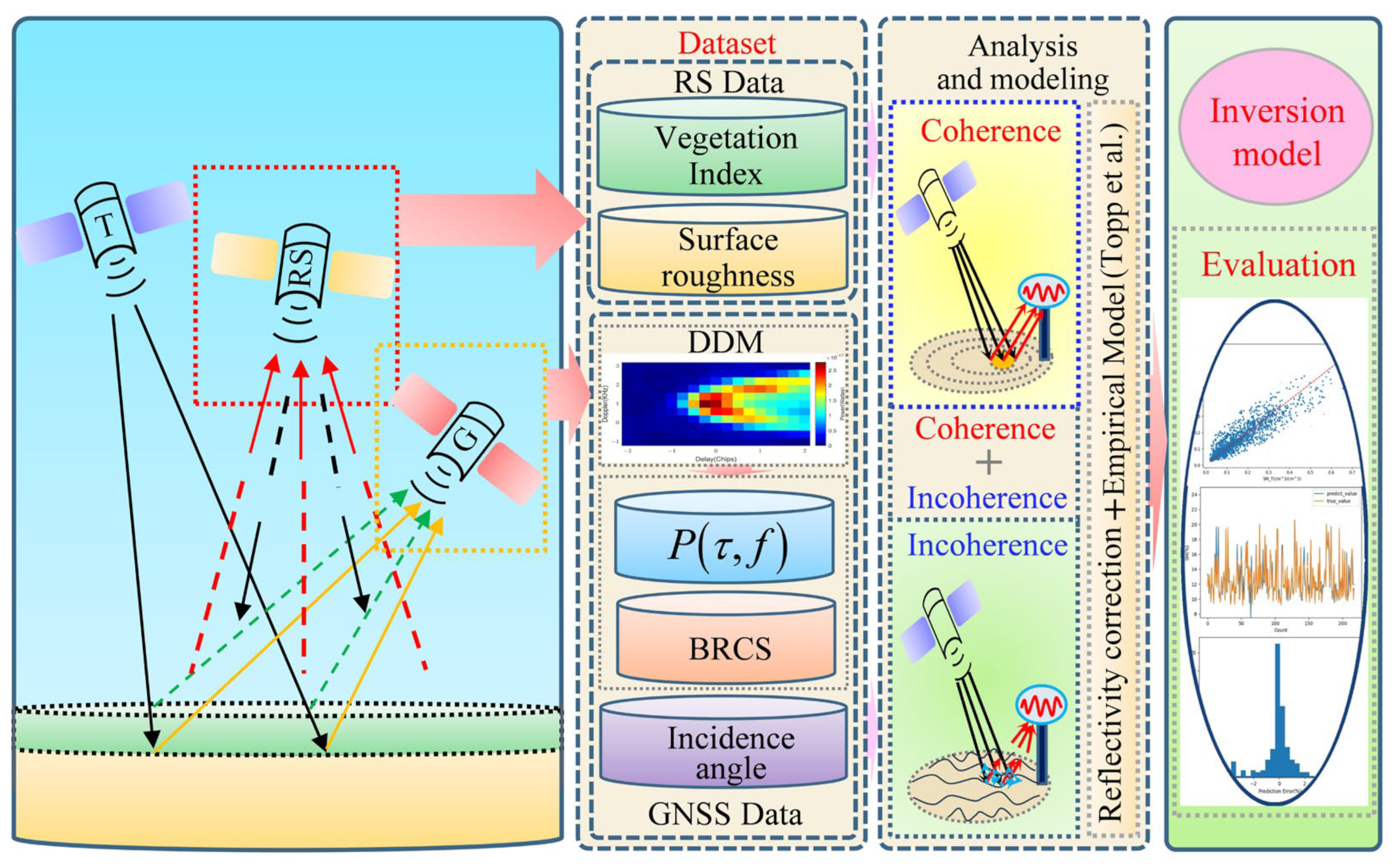
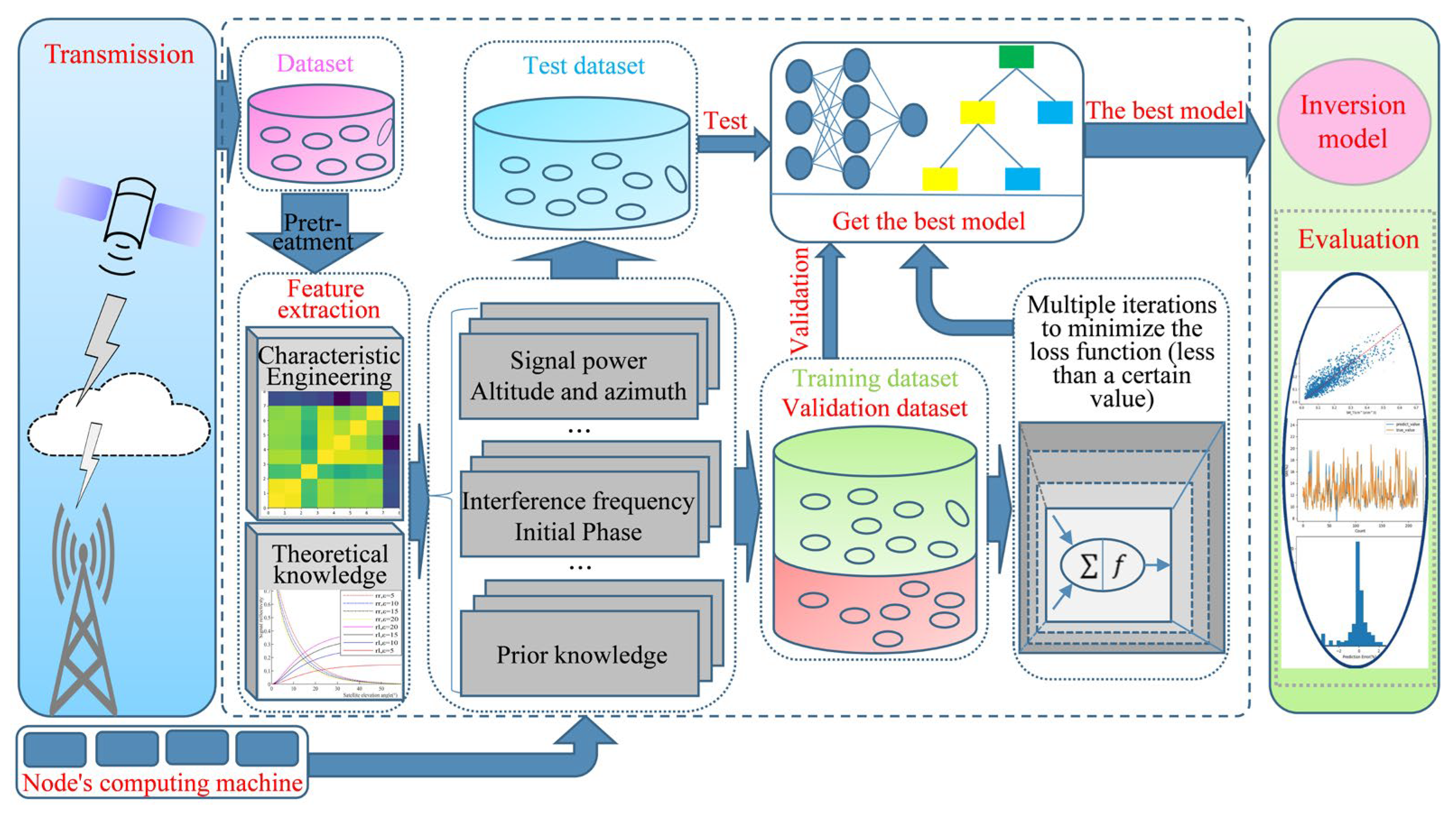
4.2. GNSS-R Soil Moisture Inversion with Machine Learning Method

ML, as a data-driven approach, has proven to be a powerful tool for environmental monitoring, using the rapidly increasing amount of remote sensing data. Compared to traditional physical and empirical models, ML methods can offer better scalability. [74]. Depending on the complexity of the model, ML methods can be classified into two categories: traditional ML methods and deep learning methods. Traditional ML methods typically include linear models, shallow neural network models, support vector machines, decision tree-based learning methods, and ensemble learning methods. These methods are generally considered simpler and more suitable for situations where the sample dataset is limited. However, they may struggle to capture the periodicity and continuity of time-series data. Deep learning models usually refer to neural network models that consist of multiple layers (typically more than three layers) and have more complex network structures. Due to the large number of network nodes in such models, a substantial amount of data is required to solve the parameters of each node during the training process. The GNSS-R SM retrieval method is essentially a process of solving a regression problem. When using a regression equation for fitting, the results are subject to considerable errors due to factors such as equation order limitations. However, ML methods can continuously approximate the actual relationship as much as possible. It typically involves five processes: data preprocessing, feature extraction, dataset splitting, model training, and model testing. The schematic diagram of constructing the GNSS-R SM inversion model with the ML method is shown in Figure 7.
Data preprocessing is a pivotal step in the development of ML models to ensure optimal performance. Key components of this process include the management of outliers and missing values, data normalization, and discretization. Among these, the handling of outliers and missing values is particularly crucial. The most effective strategies for addressing these challenges typically involve:
  • Integration of multiple data sources: Collecting various data sources to obtain more comprehensive and accurate information.
  • Data augmentation technology: Using interpolation, regression, and other methods to expand and simulate data, improving the representativeness and quantity of the dataset.
  • Modeling of spatial and temporal distributions: Establishing models of spatial and temporal distributions can effectively utilize existing data and deduce relevant information for unknown areas or time periods.
In GNSS-R SM retrieval, feature extraction is pivotal. It involves selecting observational data parameters that are closely associated with the desired outcomes for use in constructing predictive models. In the field of GNSS-R SM retrieval, the typical approach involves choosing surface reflectivity, signal strength, and incidence angle as input features. To enhance retrieval accuracy, as mentioned earlier, additional environmental characteristic parameters are being incorporated as auxiliary data in model development. These carefully selected parameters play a crucial role in capturing the fundamental information required for accurately estimating SM using GNSS-R technology. However, the effectiveness of feature selection may be impacted by feature correlation and an insufficient or excessive number of features. Therefore, it is essential to fully consider these factors during the feature selection process, and the following methods can be used:
  • Empirical analysis: Utilizing professional knowledge, domain expertise, and statistical analysis to conduct feature analysis and eliminate irrelevant features.
  • Wrapper evaluation method: This approach is a feature selection method that utilizes ML models to evaluate different subsets of features and selects the combination of features that perform best in terms of model performance.
  • Principal component analysis: Reduces dimensionality by transforming original variables into principal components. By selecting the principal components with the highest variance, important information is effectively retained, while irrelevant or redundant features are removed.
  • Embedded methods: Such as LASSO and Ridge regression, are employed directly in model construction for feature selection. These methods reduce the influence of irrelevant features by penalizing large coefficients through regularization, thereby balancing model complexity with predictive accuracy.
The process of dataset partitioning involves dividing the specified attribute and label data into training, validation, and testing sets, which are used, respectively, for model learning and testing. The training phase is the main step in ML methodologies, wherein the model iteratively adjusts its parameters to minimize the loss function, thereby optimizing performance. Effective parameter adjustment, essential for reducing the loss function, can be achieved through various methods. Traditional optimization techniques, such as simulated annealing, are commonly employed for parameter tuning. Additionally, advanced technologies, like GridSearchCV and the Optuna framework, are instrumental in hyperparameter tuning and optimization. Model testing represents the final step in obtaining an ML model, aiming to evaluate its generalization capability and performance, thereby ensuring the effectiveness of the ML model.
In general, the introduction of ML methods has significantly advanced GNSS-R SM retrieval research. Firstly, it overcomes the limitations of traditional fitting equations, avoiding approximations and the need for complex parameters in the computation process of empirical and physical models, thereby simplifying the model construction process. Moreover, they can mitigate the impact of various other factors on the GNSS-R SM inversion method, such as the inclination of the signal reflection surface and discrepancies among different signal transmission channels. These elements can be optimized as systematic errors during the model building phase.

5. Development Prospects Discussion

As is well-known, extensive research has been conducted on GNSS-R SM inversion in the past few decades, focusing on both platforms and model construction methods. Various detection modes have been developed, as depicted in Figure 8, enabling spatial monitoring resolutions that range from several meters to thousands of meters. However, it is crucial to note that, as previously mentioned, the impact of reflected signals during signal transmission encompasses multiple factors, such as SM, surface roughness, and vegetation. It is a highly intricate process and has been comprehensively described by Wu et al. in their study [75]. Currently, the analysis of vegetation effects heavily relies on ML methods or simulation models that utilize vegetation index as prior knowledge. Examples of such models include the Bi-MIMICS models [76], Water Cloud models [77], MIMICS models [78], and Clump models [79], amongst others. Furthermore, as mentioned earlier, the accuracy of the model is also affected by other factors such as elevation, slope, and soil texture, amongst others. In order to enhance the precision of the model, an increasing amount of auxiliary data is being utilized in the model construction process in current research. Nonetheless, this reliance on auxiliary data imposes limitations on the further advancement of the GNSS-R SM inversion method, impeding its progress as an independent and highly accurate SM monitoring technique. In addition, although airborne platforms can provide observations at a medium to small-scale, they may not meet the continuous long-term monitoring requirements. Therefore, it is necessary to conduct downscaling studies on spaceborne observation data. In order to further enhance the practical application ability of the GNSS-R SM remote sensing method and better supplement the SM inversion method and product, here are some potential directions for future research, summarized as follows:
(1)
Implementing multi-objective data inversion based on multi-system observation data fusion and multi-task learning (MTL) method. MTL is a TL approach that enhances model generalizability and efficiency by jointly learning across several related domains. The aim of MTL is to maximize model extrapolation and enhance performance across one or more tasks. All domains share a common feature set, while their learning tasks are distinct yet interrelated [80]. As noted, the reflectivity of GNSS signals is mainly affected by the combined influence of vegetation, surface roughness, and SM [70]. This research proposes using MTL to concurrently retrieve SM, vegetation index, and surface roughness. In theory, acquiring three target parameters simultaneously necessitates additional input features to satisfy the conditions for solving a closed system of equations. The data from FY-3E and Spire satellites present a feasible solution. These satellite systems can concurrently provide GNSS-R data from GPS, BDS, and Galileo satellites. Owing to the distinct carrier frequencies, code rates, and chip lengths of each satellite system, their respective reflection characteristics exhibit certain variances. The paper posits that the variability in these reflection characteristics can serve as a shared training set for multi-task learning, enabling the concurrent inversion of the three target parameters.
(2)
Introducing fine-tuning methods in deep learning (DL) to improve model generalization ability. ML methods are data-driven models, whose generalization capabilities are directly influenced by the training dataset. When the geographical spatial environment changes, directly applying ML models trained on the original dataset to new target tasks often results in poor performance. Therefore, current research often involves augmenting model input features with auxiliary data to accurately reflect characteristics such as the composition and spatial features of surface soil, thereby improving the model’s inversion accuracy. As is known, features like soil texture, elevation, and slope in a specific study area usually do not change significantly in the short term. In such cases, adjusting existing models for the target area can further enhance model generalization without relying on auxiliary data. The method of fine-tuning in TL is aptly suited to address this issue. Fine-tuning is a method where the model trained on a source domain is subsequently adapted to a target domain. This approach is advantageous, as it leverages existing models and data to quickly adapt to the characteristics of the target domain. In the context of deep neural networks, initial layers tend to capture general features, whereas later layers are more focused on specific tasks [81,82,83]. Therefore, in GNSS-R SM retrieval studies, researchers can freeze the weights of the initial layers of pre-trained DL architecture and fine-tune or retrain the last few layers. This customization enables the application of existing models and data to new soil types or regions, enhancing the model’s predictive capabilities.
(3)
Construction of small models based on spatiotemporal analysis and spatial feature fusion. In research areas with relatively mature and stable vegetation cover or in farmlands with consistent crop types, the vegetation indices typically exhibit distinct spatiotemporal variation characteristics. Based on the hypothesis proposed by Yin et al., which assumes that soil roughness (topography) and soil texture remain constant over time at a given location, analyzing these characteristics and segmenting them on a temporal scale to construct small models integrating spatial features can achieve accurate inversion results without relying on auxiliary data [57]. In our current research, we conducted experiments on a monthly scale and achieved favorable inversion results. It should be noted that in our study, we directly utilized the spatial location information of reflection points as input features. The results indicate that ML methods based on classifiers, such as Random Forest and XGBoost, yield good inversion outcomes. However, the use of Fully Connected Neural Networks (FCNNs) was less effective. This is attributed to the lack of a direct physical relationship between SM and the spatial location information of the reflection points. For future research, researchers can explore the construction of vegetation spatial feature indices. If an index that maps vegetation indices to spatial distributions can be developed, this concept could be applied to more model construction methods, thereby enriching the research methodologies in this field.
(4)
Deepening the research on the downscaling of spaceborne observation data. Current research in SM inversion using GNSS-R extends from ground-based to spaceborne observation models, offering spatial resolutions ranging from several meters to thousands of meters. Notably, medium to small-scale remote sensing data, primarily provided by airborne observation platforms, play a crucial role in hydrological monitoring and agricultural applications. However, it is important to note that these scales of observation, while valuable, are challenging to maintain over extended periods and large areas due to the limitations of airborne platforms. Although ground-based observation methods offer high spatial resolution, they fall short in meeting the needs for global data observation. Consequently, research on the downscaling of satellite observation data is essential. Jia et al. have developed a mapping model for CYGNSS and SMAP SM data by integrating CYGNSS data with land type, which successfully downscaled 9 km SM products to 3 km resolution. Meanwhile, the downscaled data exhibit good consistency with the corresponding in situ data [84]. As is known, SM is intricately linked to soil texture, vegetation evapotranspiration, and the spatial positioning of observation points, amongst others. To enhance the accuracy and generalizability of the downscaling model, future research could benefit from fine-tuning approaches tailored to specific target areas. In addition, Carreno-Luengo et al. have introduced an enhanced multi-scale CYGNSS data product with higher spatial resolution [85]. This advancement contributes to research on downscaling GNSS-R SM products, further enhancing the spatial resolution and accuracy of downscaled products.
Figure 8. Schematic diagram of various monitoring platforms in GNSS-R.
Remotesensing 16 01193 g008

6. Conclusions

With the development of GNSS technology, it has provided a new approach for SM retrieval by analyzing the sensitivity of its L-band signals to SM. Compared with other SM remote sensing methods, GNSS-R possesses unique advantages. For instance, unlike optical remote sensing methods that rely on clear skies, GNSS signals can penetrate clouds, fog, and even vegetation. This means that researchers can collect data continuously regardless of weather conditions, providing valuable insights into dynamic environmental processes. It also enables monitoring in regions with persistent cloud cover, such as tropical rainforests or polar regions, where other remote sensing methods may face limitations. Additionally, compared to current microwave SM remote sensing methods, its revisit time is shorter and does not require signal-emitting devices like active microwave remote sensing method, significantly reducing the research investment.
In order to improve the inversion accuracy and generalization ability of GNSS-R SM retrieval models and to enhance its practical application potential in environmental resource monitoring, hydroclimatology research, agricultural production guidance, and other fields, this paper provides a detailed review of existing research methods and prospects for future development. The paper first explains the advantages of the GNSS-R SM retrieval method over traditional SM monitoring methods, indicating the research’s importance in practical applications. Then, the existing research methods were classified into ground-based, airborne, and spaceborne modes according to different observation platforms, and a detailed review and analysis of the existing research was conducted. Furthermore, it elucidates the data processing flow, characteristics, model construction principles, and methods of different inversion techniques. Finally, the paper identifies the limitations of the current GNSS-R SM retrieval method and provides prospects for future development.

Author Contributions

Idea proposal, conceptualization, writing—original draft, writing—review and editing, C.Y.; idea proposal, conceptualization suggestions, writing—review and editing, project administration and funding acquisition, K.M.; idea proposal, conceptualization, suggestions, and review, Z.G.; conceptualization, suggestions, and review, J.S. and S.M.B.; resources and editing, Z.Y.; All authors have read and agreed to the published version of the manuscript.

Funding

This project was supported by the National Key R&D Program of China (NO.2023YFB3906202).

Data Availability Statement

Data are openly available in a public repository.

Acknowledgments

The authors would like to thank the authors of GNSS-R soil moisture inversion publications that provided us with a lot of experience.

Conflicts of Interest

The authors declare no conflicts of interest.

References

  1. Hong, S.; Shin, I. A physically-based inversion algorithm for retrieving soil moisture in passive microwave remote sensing. J. Hydrol. 2011, 405, 24–30. [Google Scholar] [CrossRef]
  2. Jin, S.; Feng, G.; Gleason, S. Remote sensing using GNSS signals: Current status and future directions. Adv. Space Res. 2011, 47, 1645–1653. [Google Scholar] [CrossRef]
  3. May, W.; Rummukainen, M.; Cheruy, F.; Hagemann, S.; Meier, A. Contributions of soil moisture interactions to future precipitation changes in the GLACE-CMIP5 experiment. Clim. Dynam. 2017, 49, 1681–1704. [Google Scholar] [CrossRef]
  4. Vogel, M.M.; Zscheischler, J.; Seneviratne, S.I. Varying soil moisture-atmosphere feedbacks explain divergent temperature extremes and precipitation projections in central Europe. Earth Syst. Dynam. 2018, 9, 1107–1125. [Google Scholar] [CrossRef]
  5. Lekshmi, S.U.S.; Singh, D.N.; Baghini, M.S. A critical review of soil moisture measurement. Measurement 2014, 54, 92–105. [Google Scholar] [CrossRef]
  6. Orth, S.; Orth, R. Global Soil Moisture Data Derived through Machine Learning Trained with In-Situ Measurements. Sci. Data 2021, 8, 170. [Google Scholar] [CrossRef]
  7. Malicki, M.A.; Skierucha, W.M. A manually controlled TDR soil moisture meter operating with 300 ps rise-time needle pulse. Irrig. Sci. 1989, 10, 153–163. [Google Scholar] [CrossRef]
  8. Saradjian, M.R. Comparison of Optical, Radar, and Hybrid Soil Moisture Estimation Models Using Experimental Data. J. Appl. Remote Sens. 2011, 5, 053524. [Google Scholar] [CrossRef]
  9. Entekhabi, D.; Njoku, E.G.; O’Neill, P.E.; Kellogg, K.H.; Crow, W.T.; Edelstein, W.N.; Entin, J.K.; Goodman, S.D.; Jackson, T.J.; Johnson, J.; et al. The Soil Moisture Active Passive (SMAP) Mission. Proc. IEEE 2010, 98, 704–716. [Google Scholar] [CrossRef]
  10. Kornelsen, K.C.; Coulibaly, P. Advances in Soil Moisture Retrieval from Synthetic Aperture Radar and Hydrological Applications. J. Hydrol. 2013, 476, 460–489. [Google Scholar] [CrossRef]
  11. Jackson, T.J. III. Measuring surface soil moisture using passive microwave remote sensing. Hydrol. Process. 1993, 7, 139–152. [Google Scholar] [CrossRef]
  12. Davenport, I.J.; Fernandez-Galvez, J.; Gurney, R.J. A sensitivity analysis of soil moisture retrieval from the Tau-Omega microwave emission model. IEEE Trans. Geosci. Remote Sens. 2005, 43, 1304–1316. [Google Scholar] [CrossRef]
  13. Kerr, Y.H.; Waldteufel, P.; Richaume, P.; Wigneron, J.P.; Ferrazzoli, P.; Mahmoodi, A.; Al Bitar, A.; Cabot, F.; Gruhier, C.; Juglea, S.E.; et al. The SMOS Soil Moisture Retrieval Algorithm. IEEE Trans. Geosci. Remote Sens. 2012, 50, 1384–1403. [Google Scholar] [CrossRef]
  14. Martin-Neira, M. A passive reflectometry and interferometry system (PARIS): Application to ocean altimetry. ESA J. 1993, 17, 331–355. [Google Scholar]
  15. Roussel, N.; Frappart, F.; Ramillien, G. Simulations of direct and reflected waves trajectories for in situ GNSS-R experiments. Geosci. Model Develop. 2014, 7, 2261–2279. [Google Scholar] [CrossRef]
  16. Ribot, M.A.; Botteron, C.; Farine, P.A. Derivation of the Cramér-Rao Bound in the GNSS-Reflectometry Context for Static, Ground-Based Receivers in Scenarios with Coherent Reflection. Sensors 2016, 16, 2063. [Google Scholar] [CrossRef] [PubMed]
  17. Rahmani, M.; Asgari, J.; Milad, S. Soil moisture retrieval using space-borne GNSS reflectometry: A comprehensive review. Int. J. Remote Sens. 2022, 43, 5173–5203. [Google Scholar] [CrossRef]
  18. Zavorotny, V.U.; Voronovich, A.G. Bistatic GPS Signal Reflections at Various Polarizations from Rough Land Surface with Moisture Content. In Proceedings of the IEEE 2000 International Geoscience and Remote Sensing Symposium, Honolulu, HI, USA, 24–28 July 2000. [Google Scholar]
  19. Egido, A.; Ruffini, G.; Caparrini, M.; Martin, C.; Farrés, E.; Banque, X. Soil Moisture Monitorization Using GNSS Reflected Signals. In Proceedings of the 1st Colloquium Scientific and Fundamental Aspects of the Galileo Programme, Toulouse, France, 1–4 October 2007. [Google Scholar]
  20. Jia, Y.; Jin, S.; Savi, P.; Yan, Q.; Li, W. Modeling and Theoretical Analysis of GNSS-R Soil Moisture Retrieval Based on the Random Forest and Support Vector Machine Learning Approach. Remote Sens. 2020, 12, 3679. [Google Scholar] [CrossRef]
  21. Larson, K.M.; Small, E.E.; Gutmann, E.; Bilich, A.; Axelrad, P.; Braun, J. Using GPS multipath to measure soil moisture fluctuations: Initial results. GPS Solut. 2008, 12, 173–177. [Google Scholar] [CrossRef]
  22. Larson, K.M.; Small, E.E.; Gutmann, E.D.; Bilich, A.L.; Braun, J.J.; Zavorotny, V.U. Use of GPS receivers as a soil moisture network for water cycle studies. Geophys. Res. Lett. 2008, 35, L24405. [Google Scholar] [CrossRef]
  23. Larson, K.M.; Braun, J.J.; Small, E.E.; Zavorotny, V.U.; Gutmann, E.D.; Bilich, A.L. GPS Multipath and Its Relation to Near-Surface Soil Moisture Content. IEEE J. Sel. Top. Appl. Earth Obs. Remote Sens. 2010, 3, 91–99. [Google Scholar] [CrossRef]
  24. Sibylle, V.; Andreas, G.; Jens, W.; Theresa, B.; Markus, R. Long-term soil moisture dynamics derived from GNSS interferometric reflectometry: A case study for Sutherland, South Africa. Gps Solut. 2016, 20, 641–654. [Google Scholar] [CrossRef]
  25. Rodriguez-Alvarez, N.; Bosch-Lluis, X.; Camps, A.; Vall-llossera, M.; Valencia, E.; Marchan-Hernandez, J.F.; Ramos-Perez, I. Soil Moisture Retrieval Using GNSS-R Techniques: Experimental Results Over a Bare Soil Field. IEEE Trans. Geosci. Remote Sens. 2009, 47, 3616–3624. [Google Scholar] [CrossRef]
  26. Rodriguez-Alvarez, N.; Camps, A.; Vall-llossera, M.; Bosch-Lluis, X.; Monerris, A.; Ramos-Perez, I.; Valencia, E.; Marchan-Hernandez, J.F.; Martinez-Fernandez, J.; Baroncini-Turricchia, G.; et al. Land Geophysical Parameters Retrieval Using the Interference Pattern GNSS-R Technique. IEEE Trans. Geosci. Remote Sens. 2011, 49, 71–84. [Google Scholar] [CrossRef]
  27. Zhang, S.; Calvet, J.-C.; Darrozes, J.; Roussel, N.; Frappart, F.; Bouhours, G. Deriving Surface Soil Moisture from Reflected GNSS Signal Observations from a Grassland Site in Southwestern France. Hydrol. Earth Syst. Sci. 2018, 22, 1931–1946. [Google Scholar] [CrossRef]
  28. Zhang, S.; Roussel, N.; Boniface, K.; Ha, M.C.; Frappart, F.; Darrozes, J.; Baup, F.; Calvet, J.-C. Use of Reflected GNSS SNR Data to Retrieve Either Soil Moisture or Vegetation Height from a Wheat Crop. Hydrol. Earth Syst. Sci. 2017, 21, 4767–4784. [Google Scholar] [CrossRef]
  29. Jing, L.; Yang, L.; Yang, W.; Xu, T.; Gao, F.; Lu, Y.; Sun, B.; Yang, D.; Hong, X.; Wang, N.; et al. Robust Kalman Filter Soil Moisture Inversion Model Using GPS SNR Data—A Dual-Band Data Fusion Approach. Remote Sens. 2021, 13, 4013. [Google Scholar] [CrossRef]
  30. Ha, M.-C.; Darrozes, J.; Llubes, M.; Grippa, M.; Ramillien, G.; Frappart, F.; Baup, F.; Tagesson, H.T.; Mougin, E.; Guiro, I.; et al. GNSS-R Monitoring of Soil Moisture Dynamics in Areas of Severe Drought: Example of Dahra in the Sahelian Climatic Zone (Senegal). Eur. J. Remote Sens. 2023, 56, 2156931. [Google Scholar] [CrossRef]
  31. Masters, D.; Axelrad, P.; Katzberg, S. Initial results of land-reflected GPS bistatic radar measurements in SMEX02. Remote Sens. Environ. 2004, 92, 507–520. [Google Scholar] [CrossRef]
  32. Katzberg, S.J.; Torres, O.; Grant, M.S.; Masters, D. Utilizing calibrated GPS reflected signals to estimate soil reflectivity and dielectric constant: Results from SMEX02. Remote Sens. Environ. 2006, 100, 17–28. [Google Scholar] [CrossRef]
  33. Munoz-Martin, J.F.; Onrubia, R.; Pascual, D.; Park, H.; Pablos, M.; Camps, A.; Rüdiger, C.; Walker, J.; Monerris, A. Single-Pass Soil Moisture Retrieval Using GNSS-R at L1 and L5 Bands: Results from Airborne Experiment. Remote Sens. 2021, 13, 797. [Google Scholar] [CrossRef]
  34. Oudrhiri, K.; Rodriguez-Alvarez, N.; Yang, Y.-M.; Lay, N.E.; Buccino, D.; Shin, D.; Podest, E.; Brockers, R. Bistatic Radar Experiments with UAV: Qualification and Performance of a Miniaturized Instrument. In Proceedings of the 2021 IEEE Aerospace Conference (50100), Big Sky, MT, USA, 6–13 March 2021. [Google Scholar]
  35. Moller, D.; Ruf, C.; Linnabary, R.; O’Brien, A.; Musko, S. Operational Airborne GNSS-R Aboard Air New Zealand Domestic Aircraft. In Proceedings of the 2021 IEEE International Geoscience and Remote Sensing Symposium IGARSS, Brussels, Belgium, 11–16 July 2021. [Google Scholar]
  36. Gleason, S.; Adjrad, M. Sensing Ocean, Ice and Land Reflected Signals from Space: Results from the UK-DMC GPS Reflectometry Experiment. In Proceedings of the 18th International Technical Meeting of the Satellite Division of The Institute of Navigation, Long Beach, CA, USA, 13–16 September 2005. [Google Scholar]
  37. Unwin, M.; Jales, P.; Tye, J.; Gommenginger, C.; Foti, G.; Rosello, J. Spaceborne GNSS-Reflectometry on TechDemoSat-1: Early Mission Operations and Exploitation. IEEE J. Sel. Top. Appl. Earth Obs. Remote Sens. 2016, 9, 4525–4539. [Google Scholar] [CrossRef]
  38. Ruf, C.; Asharaf, S.; Balasubramaniam, R.; Gleason, S.; Lang, T.; Mckague, D.; Twigg, D.; Waliser, D. In-Orbit Performance of the Constellation of CYGNSS Hurricane Satellites. Bull. Am. Meteorol. Soc. 2019, 100, 2009–2023. [Google Scholar] [CrossRef]
  39. Guo, Z.; Liu, B.; Wan, W.; Lu, F.; Niu, X.; Ji, R.; Jing, C.; Li, W.; Chen, X.; Yang, J.; et al. Soil Moisture Retrieval Using BuFeng-1 A/B Based on Land Surface Clustering Algorithm. IEEE J. Sel. Top. Appl. Earth Obs. Remote Sens. 2022, 15, 4680–4689. [Google Scholar] [CrossRef]
  40. Munoz-Martin, J.F.; Fernandez-Capon, L.; Ruiz-de-Azua, J.; Camps, A. The Flexible Microwave Payload-2: A SDR-Based GNSS-Reflectometer and L-Band Radiometer for CubeSats. IEEE J. Sel. Top. Appl. Earth Obs. Remote Sens. 2020, 13, 1298–1311. [Google Scholar] [CrossRef]
  41. Sun, Y.; Liu, C.; Du, Q.; Wang, X.; Liu, C. Global navigation satellite system occultation sounder II (GNOS II). In Proceedings of the 2017 IEEE International Geoscience and Remote Sensing Symposium (IGARSS), Fort Worth, TX, USA, 23–28 July 2017. [Google Scholar]
  42. Setti, P.T.; Tabibi, S. Evaluation of Spire GNSS-R Reflectivity from Multiple GNSS Constellations for Soil Moisture Estimation. Int. J. Remote Sens. 2023, 44, 6422–6441. [Google Scholar] [CrossRef]
  43. Camps, A.; Park, H.; Pablos, M.; Foti, G.; Gommenginger, C.P.; Liu, P.W.; Judge, J. Sensitivity of GNSS-R Spaceborne Observations to Soil Moisture and Vegetation. IEEE J. Sel. Top. Appl. Earth Obs. Remote Sens. 2016, 9, 4730–4742. [Google Scholar] [CrossRef]
  44. Chew, C.; Shah, R.; Zuffada, C.; Hajj, G.; Masters, D.; Mannucci, A.J. Demonstrating soil moisture remote sensing with observations from the UK TechDemoSat-1 satellite mission. Geophys. Res. Lett. 2016, 43, 3317–3324. [Google Scholar] [CrossRef]
  45. Jia, Y.; Jin, S.; Yan, Q.; Savi, P.; Zhang, R.; Li, W. An Effective Land Type Labeling Approach for Independently Exploiting High-Resolution Soil Moisture Products Based on CYGNSS Data. IEEE J. Sel. Top. Appl. Earth Obs. Remote Sens. 2022, 15, 4234–4247. [Google Scholar] [CrossRef]
  46. Chew, C.C.; Small, E.E. Soil Moisture Sensing Using Spaceborne GNSS Reflections: Comparison of CYGNSS Reflectivity to SMAP Soil Moisture. Geophys. Res. Lett. 2018, 45, 4049–4057. [Google Scholar] [CrossRef]
  47. Kim, H.; Lakshmi, V. Use of Cyclone Global Navigation Satellite System (CyGNSS) Observations for Estimation of Soil Moisture. Geophys. Res. Lett. 2018, 45, 8272–8282. [Google Scholar] [CrossRef]
  48. Wan, W.; Liu, B.; Guo, Z.; Lu, F.; Niu, X.; Li, H.; Ji, R.; Cheng, J.; Li, W.; Chen, X.; et al. Initial Evaluation of the First Chinese GNSS-R Mission BuFeng-1 A/B for Soil Moisture Estimation. IEEE Geosci. Remote Sens. Lett. 2022, 19, 8017305. [Google Scholar] [CrossRef]
  49. Al-Khaldi, M.M.; Johnson, J.T.; O’Brien, A.J.; Balenzano, A.; Mattia, F. Time-Series Retrieval of Soil Moisture Using CYGNSS. IEEE Trans. Geosci. Remote Sens. 2019, 57, 4322–4331. [Google Scholar] [CrossRef]
  50. Munoz-Martin, J.F.; Llaveria, D.; Herbert, C.; Pablos, M.; Park, H.; Camps, A. Soil Moisture Estimation Synergy Using GNSS-R and L-Band Microwave Radiometry Data from FSSCat/FMPL-2. Remote Sens. 2021, 13, 994. [Google Scholar] [CrossRef]
  51. Santi, E.; Pettinato, S.; Paloscia, S.; Clarizia, M.P.; Dente, L.; Guerriero, L.; Comite, D.; Pierdicca, N. Soil Moisture and Forest Biomass retrieval on a global scale by using CyGNSS data and Artificial Neural Networks. In Proceedings of the IEEE International Geoscience and Remote Sensing Symposium, Waikoloa, HI, USA, 26 September–2 October 2020. [Google Scholar]
  52. Yan, Q.; Jin, S.; Huang, W.; Jia, Y. Global Soil Moisture Estimation Using CYGNSS Data. In Proceedings of the IGARSS 2020—2020 IEEE International Geoscience and Remote Sensing Symposium, Waikoloa, HI, USA, 26 September 2020. [Google Scholar]
  53. Yang, T.; Wan, W.; Sun, Z.; Liu, B.; Li, S.; Chen, X. Comprehensive Evaluation of Using TechDemoSat-1 and CYGNSS Data to Estimate Soil Moisture over Mainland China. Remote Sens. 2020, 12, 1699. [Google Scholar] [CrossRef]
  54. Jia, Y.; Jin, S.; Chen, H.; Yan, Q.; Savi, P.; Jin, Y.; Yuan, Y. Temporal-Spatial Soil Moisture Estimation from CYGNSS Using Machine Learning Regression with a Preclassification Approach. IEEE J. Sel. Top. Appl. Earth Obs. Remote Sens. 2021, 14, 4879–4893. [Google Scholar] [CrossRef]
  55. Zhu, Y.; Guo, F.; Zhang, X. Effect of Surface Temperature on Soil Moisture Retrieval Using CYGNSS. Int. J. Appl. Earth Obs. Geoinf. 2022, 112, 102929. [Google Scholar] [CrossRef]
  56. Zhang, S.; Guo, Q.; Liu, Q.; Ma, Z.; Liu, N.; Hu, S.; Bao, L.; Zhou, X.; Zhao, H.; Wang, L.; et al. Improvement of CYGNSS Soil Moisture Retrieval Model Considering Water and Surface Temperature. Adv. Space Res. 2023, 72, 3048–3064. [Google Scholar] [CrossRef]
  57. Yin, C.; Huang, F.; Xia, J.; Bai, W.; Sun, Y.; Yang, G.; Zhai, X.; Xu, N.; Hu, X.; Zhang, P.; et al. Soil Moisture Retrieval from Multi-GNSS Reflectometry on FY-3E GNOS-II by Land Cover Classification. Remote Sens. 2023, 15, 1097. [Google Scholar] [CrossRef]
  58. Jia, Y.; Pei, Y. Remote Sensing in Land Applications by Using GNSS-Reflectometry. In Recent Advances and Applications in Remote Sensing; Hung, M.-C., Wu, Y.-H., Eds.; IntechOpen: London, UK, 2018. [Google Scholar]
  59. Han, M.; Zhu, Y.; Yang, D.; Chang, Q.; Hong, X.; Song, S. Soil moisture monitoring using GNSS interference signal: Proposing a signal reconstruction method. Remote Sens. Lett. 2020, 11, 373–382. [Google Scholar] [CrossRef]
  60. Kavak, A.; Vogel, W.J.; Xu, G.H. Using GPS To Measure Ground Complex Permittivity. Electron. Lett. 1998, 34, 254–255. [Google Scholar] [CrossRef]
  61. Peng, X.; Wan, W.; Chen, X. Using GPS SNR Data to Estimate Soil Moisture Variations: Proposing a New Interference Model. In Proceedings of the IEEE International Geoscience and Remote Sensing Symposium (IGARSS), Beijing, China, 10–15 July 2016. [Google Scholar]
  62. Yang, T.; Wan, W.; Chen, X.; Chu, T.; Hong, Y. Using BDS SNR Observations to Measure Near-Surface Soil Moisture Fluctuations: Results from Low Vegetated Surface. IEEE Geosci. Remote Sens. Lett. 2017, 14, 1308–1312. [Google Scholar] [CrossRef]
  63. Han, M.; Zhu, Y.; Yang, D.; Hong, X.; Song, S. A Semi-Empirical SNR Model for Soil Moisture Retrieval Using GNSS SNR Data. Remote Sens. 2018, 10, 280. [Google Scholar] [CrossRef]
  64. Wang, J.R.; Schmugge, T.J. An Empirical Model for the Complex Dielectric Permittivity of Soils as a Function of Water Content. IEEE Trans. Geosci. Remote Sens. 1980, GE-18, 288–295. [Google Scholar] [CrossRef]
  65. Topp, G.C.; Davis, J.L.; Annan, A.P. Electromagnetic determination of soil water content: Measurements in coaxial transmission lines. Water Resour. Res. 1980, 16, 574–582. [Google Scholar] [CrossRef]
  66. Dobson, M.C.; Ulaby, F.T.; Hallikainen, M.T.; El-rayes, M.A. Microwave Dielectric Behavior of Wet Soil-Part II:Dielectric Mixing Models. IEEE Trans. Geosci. Remote Sens. 1985, GE-23, 35–46. [Google Scholar] [CrossRef]
  67. Hallikainen, M.T.; Ulaby, F.T.; Dobson, M.C.; El-rayes, M.A. Microwave Dielectric Behavior of Wet Soil-Part 1: Empirical Models and Experimental Observations. IEEE Trans. Geosci. Remote Sens. 1985, GE-23, 25–34. [Google Scholar] [CrossRef]
  68. Balakhder, A.M.; Al-Khaldi, M.M.; Johnson, J.T. On the Coherency of Ocean and Land Surface Specular Scattering for GNSS-R and Signals of Opportunity Systems. IEEE Trans. Geosci. Remote Sens. 2019, 57, 10426–10436. [Google Scholar] [CrossRef]
  69. Campbell, J.D.; Akbar, R.; Bringer, A.; Comite, D.; Dente, L.; Gleason, S.T.; Guerriero, L.; Hodges, E.; Johnson, J.T.; Kim, S.-B.; et al. Intercomparison of Electromagnetic Scattering Models for Delay-Doppler Maps Along a CYGNSS Land Track with Topography. IEEE Trans. Geosci. Remote Sens. 2022, 60, 2007413. [Google Scholar] [CrossRef]
  70. Yueh, S.H.; Shah, R.; Chaubell, M.J.; Hayashi, A.; Xu, X.L.; Colliander, A. A Semiempirical Modeling of Soil Moisture, Vegetation, and Surface Roughness Impact on CYGNSS Reflectometry Data. IEEE Trans. Geosci. Remote Sens. 2022, 60, 5800117. [Google Scholar] [CrossRef]
  71. Wu, X.; Ma, W.; Xia, J.; Bai, W.; Jin, S.; Calabia, A. Spaceborne GNSS-R Soil Moisture Retrieval: Status, Development Opportunities, and Challenges. Remote Sens. 2021, 13, 45. [Google Scholar] [CrossRef]
  72. Campbell, J.D.; Melebari, A.; Moghaddam, M. Modeling the Effects of Topography on Delay-Doppler Maps. IEEE J. Sel. Top. Appl. Earth Obs. Remote Sens. 2020, 13, 1740–1751. [Google Scholar] [CrossRef]
  73. Turner, R.; Panciera, R.; Tanase, M.A.; Lowell, K.; Hacker, J.M.; Walker, J.P. Estimation of soil surface roughness of agricultural soils using airborne LiDAR. Remote Sens. Environ. 2014, 140, 107–117. [Google Scholar] [CrossRef]
  74. Ma, Y.; Chen, S.; Ermon, S.; Lobell, D.B. Transfer Learning in Environmental Remote Sensing. Remote Sens. Environ. 2024, 301, 113924. [Google Scholar] [CrossRef]
  75. Wu, X.; Wang, F. LAGRS-Veg: A Spaceborne Vegetation Simulator for Full Polarization GNSS-Reflectometry. GPS Solut. 2023, 27, 107. [Google Scholar] [CrossRef]
  76. Wu, X.; Li, Y.; Li, C. Bi-Mimics of Different Polarizations in Order for GNSS-R Polarimetry. Energy Procedia 2012, 16, 451–456. [Google Scholar] [CrossRef]
  77. Attema, E.P.W.; Ulaby, F.T. Vegetation modeled as a water cloud. Radio Sci. 1978, 13, 357–364. [Google Scholar] [CrossRef]
  78. Ulaby, F.T.; Sarabandi, K.; McDonald, K. Michigan Microwave Canopy Scattering Model. Int. J. Remote Sens. 1990, 11, 1223–1253. [Google Scholar] [CrossRef]
  79. Chauhan, N.S.; Lang, R.H. Radar Backscattering from Alfalfa Canopy: A Clump Modeling Approach. Int. J. Remote Sens. 1999, 20, 2203–2220. [Google Scholar] [CrossRef]
  80. Zhang, Y.; Yang, Q. A Survey on Multi-Task Learning. IEEE Trans. Knowl. Data Eng. 2022, 34, 5586–5609. [Google Scholar] [CrossRef]
  81. Gadiraju, K.K.; Vatsavai, R.R. Comparative Analysis of Deep Transfer Learning Performance on Crop Classification. In Proceedings of the 9th ACM SIGSPATIAL International Workshop on Analytics for Big Geospatial Data, Seattle, WA, USA, 3 November 2020. [Google Scholar]
  82. Wang, A.X.; Tran, C.; Desai, N.; Lobell, D.; Ermon, S. Deep Transfer Learning for Crop Yield Prediction with Remote Sensing Data. In Proceedings of the 1st ACM SIGCAS Conference on Computing and Sustainable Societies, San Jose, CA USA, 20 June 2018. [Google Scholar]
  83. Abdalla, A.; Cen, H.; Wan, L.; Rashid, R.; Weng, H.; Zhou, W.; He, Y. Fine-Tuning Convolutional Neural Network with Transfer Learning for Semantic Segmentation of Ground-Level Oilseed Rape Images in a Field with High Weed Pressure. Comput. Electron. Agric. 2019, 167, 105091. [Google Scholar] [CrossRef]
  84. Jia, Y.; Zou, J.; Jin, S.; Yan, Q.; Chen, Y.; Jin, Y.; Savi, P. Multiresolution Soil Moisture Products Based on a Spatially Adaptive Estimation Model and CYGNSS Data. GISci. Remote Sens. 2024, 61, 2313812. [Google Scholar] [CrossRef]
  85. Carreno-Luengo, H.; Ruf, C.S.; Gleason, S.; Russel, A. A New Multiresolution CYGNSS Data Product for Fully and Partially Coherent Scattering. IEEE Trans. Geosci. Remote Sens. 2023, 61, 4408118. [Google Scholar] [CrossRef]
Figure 1. GNSS satellite signal propagation diagram.
Remotesensing 16 01193 g001
Figure 2. Schematic diagram of reflectivity variation.
Remotesensing 16 01193 g002
Figure 3. (a) Diagram of the classic double-slit interference experiment. (b) Schematic diagram of signal propagation and reception in the GNSS-IR SM inversion method.
Remotesensing 16 01193 g003
Figure 4. Technical roadmap of GNSS-IR methods and key technologies.
Remotesensing 16 01193 g004
Figure 6. Schematic diagram of SM inversion using the spaceborne GNSS-R method.
Remotesensing 16 01193 g006
Figure 7. Schematic diagram of the GNSS-R SM inversion model with the ML method.
Remotesensing 16 01193 g007
Table 1. Examples of spaceborne GNSS-R SM inversion studies 1.
Study MissionSatellitesSpatial CoverageMain ComponentsGNSS DataAuxiliary DataAdopted AlgorithmsReference SMValidation SMMain Results (cm3/cm3)
Chew and small [46]CYGNSSQuasi-GlobalCoherentReflectivityLAILinear
regression
SMAPSMAP, in situmedian ubRMSE = 0.045
Kim and Lakshmi [47]CYGNSSRegional
(CONUS)
CoherentReflectivityGPM, VWC, landcover typesLinear
regression
SMAPSMAPFor different observation
conditions: R = 0.67/0.68/0.77
Wan et al. [48]BuFeng-1 A/BQuasi-GlobalBoth ReflectivityVWCLinear
regression
SMAPSMAP, in situR = 0.94, RMSE = 0.029
(vs. SMAP)
R = 0.77, RMSE = 0.049
(vs. in situ)
Al-Khaldi et al. [49]CYGNSSQuasi-GlobalIncoherentBRCSTime-Series techniqueSMAPSMAPR = 0.82, RMSE = 0.04
Munoz-Martin et al. [50]FSSCatRegional
(above 45°N)
CoherentReflectivity,
SNR, incident angle
FMPL-2 MWR radiometry dataANNSMOSSMOSR = 0.79,
STD (error) = 0.063
Santi et al. [51]CYGNSSQuasi-GlobalReflectivity, SNR, incident angleVODANNSMAPSMAPR = 0.85, RMSE = 0.069
Yan et al. [52]CYGNSSQuasi-GlobalCoherentReflectivity (maximum, mean,
variance, skewness,
kurtosis)
VODLinear
regression
SMAPSMAPR = 0.80,
RMSE = 0.07
Yang et al. [53]TDS-1,
CYGNSS
Regional
(China)
CoherentReflectivityElevation, slope, NDVI, VWC, roughness data, precipitationBP-ANNSMAPSMAP, in situR = 0.676/0.798,
ubRMSE = 0.060/0.062,
MAE = 0.052/0.040
(TDS-1/CYGNSS vs. SMAP)
R = 0.687/0.724,
ubRMSE = 0.056/0.053,
MAE = 0.066/0.052
(TDS-1/CYGNSS vs. in situ)
Jia et al. [54]CYGNSSQuasi-GlobalCoherent ReflectivityVOD,
roughness coefficient
XGBoost with pre-classification strategySMAPSMAP, in situmedian RMSE = 0.052,
median R = 0.86
(vs. SMAP)
median RMSE = 0.049,
median R = 0.753
(vs. in situ)
Jia et al. [45]CYGNSSQuasi-GlobalCoherentReflectivity, TES, dielectric constant, incident angleLand typeXGBoost with an LT digitization strategySMAPSMAPR = 0.71, RMSE = 0.063
Zhu et al. [55]CYGNSSQuasi-GlobalCoherentReflectivityVOD, SSTLinear
regression
SMAPSMAP, in situR = 0.929, RMSE = 0.043
(vs. SMAP)
R = 0.927, RMSE = 0.042
(vs. in situ)
Zhang et al. [56]CYGNSSRegional
(CONUS)
CoherentReflectivity (maximum, mean, variance, skewness,
kurtosis)
VOD, SSTLinear
regression
SMAPSMAP, in situR = 0.815, RMSE = 0.066
(vs. SMAP)
R = 0.549, RMSE = 0.078
(vs. in situ)
Yin et al. [57]FY-3EGlobalCoherentReflectivity
(GPS/BDS/GAL)
VWC,
IGBP classification
Linear
regression
SMAPSMAP, in situR = 0.83/0.85/0.86,
RMSE = 0.0503/0.0497/0.0482
(GPS/BDS/GAL vs. SMAP)
Mean RMSE = 0.054
(GPS/BDS/GAL vs. in situ)
Setti. et al. [42]SpireRegional
(Southeast Australia)
CoherentReflectivity
(GPS/multi)
Linear
regression
SMAPSMAP, in situR = 0.85,
median ubRMSE = 0.062
(Spire-multi vs. SMAP)
median ubRMSE = 0.057
(Spire-multi vs. in situ)
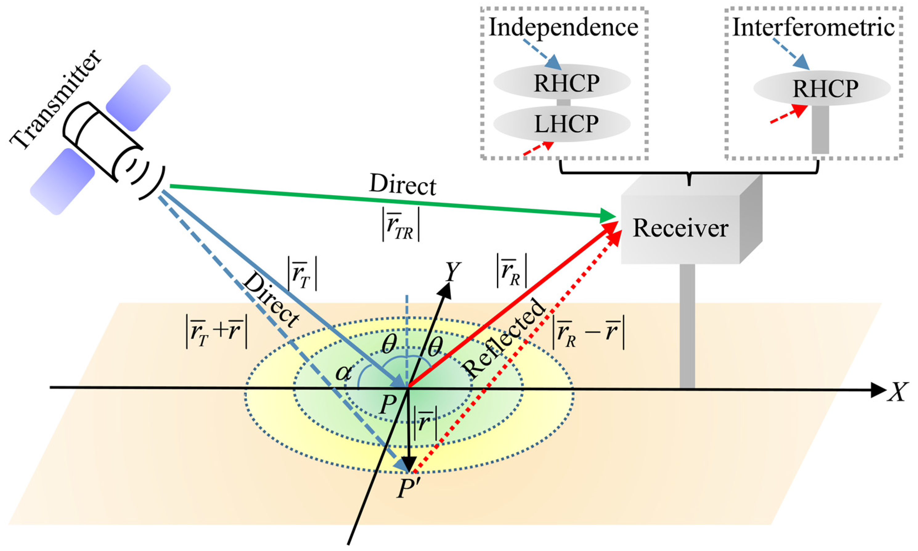
1 LAI: leaf area index; GPM: global precipitation measurement; VWC: vegetation water content; NDVI: normalized difference vegetation index; VOD: vegetation optical depth; SST: soil surface temperature.
Table 2. Differences in SM inversion by receiving reflection signals in different ways.
Receive WaysMechanizationAdvantageDeficiencyApplicable Platforms
IndependenceIndependently receiving signals, and the model is built based on reflectanceIntuitively acquiring signal characteristicsRequires specific equipmentGround-based,
Airborne,
Spaceborne
InterferometricReceiving interference signals, and the model is established based on its characteristicsDoes not require specific equipmentRequires data processing algorithmsGround-based
Table 3. The values of μ and ν in samples of Hallikainen et al.’s experiment [67].
Soil Type μ / % ν / %
Sandy Loam51.5113.43
Loam41.968.53
Silt Loam30.6313.48
Silty Clay5.0247.38
Disclaimer/Publisher’s Note: The statements, opinions and data contained in all publications are solely those of the individual author(s) and contributor(s) and not of MDPI and/or the editor(s). MDPI and/or the editor(s) disclaim responsibility for any injury to people or property resulting from any ideas, methods, instructions or products referred to in the content.

