Abstract
Development of ocean measurement technologies can improve monitoring of the global Ocean Heat Content (OHC) and Heat Storage Rate (HSR) that serve as early-warning indices for climate-critical circulation processes such as the Atlantic Meridional Overturning Circulation and provide real-time OHC assessments for tropical cyclone forecast models. This paper examines the potential of remotely measuring ocean temperature profiles using a simulated Brillouin lidar for calculating ocean HSR. A series of data analysis (‘Nature’) and Observational Systems Simulation Experiments (OSSEs) were carried out using 26 years (1992–2017) of daily mean temperature and salinity outputs from the ECCOv4r4 ocean circulation model. The focus of this study is to compare various OSSEs carried out to measure the HSR using a simulated Brillouin lidar against the HSR calculated from the ECCOv4r4 model results. Brillouin lidar simulations are used to predict the probability of detecting a return lidar signal under varying sampling strategies. Correlations were calculated for the difference between sampling strategies. These comparisons ignore the measurement errors inherent in a Brillouin lidar. Brillouin lidar technology and instruments are known to contain numerous, instrument-dependent errors and remain an engineering challenge. A significant decrease in the ability to measuring global ocean HSRs is a consequence of measuring ocean temperature from nadir-pointing instruments that can only take measurements along-track. Other sources of errors include the inability to fully profile ocean regions with deep mixed layers, such as the Southern Ocean and North Atlantic, and ocean regions with high light attenuation levels.
1. Introduction
The Earth’s oceans have stored away more than 90 percent of the additional heat absorbed by the planet due to anthropogenic changes to Earth, primarily from elevated levels of greenhouse gases [1,2]. The resulting alterations in ocean temperature and associated heat content has and will continue to influence global climate [3], alter ocean circulation and biogeochemistry [4,5], and impact ocean ecosystems [6,7,8] until at least 2300 [5]. How ocean temperatures respond to global warming is the topic of numerous scientific papers [3], field studies such as the global Argo network [9,10], the National Oceanic and Atmospheric (NOAA) surface drifter [11,12] and high-density eXpendable BathyThermograph (XBT) programs [13], and numerical simulations [14].
The ability to measure the vertical structure of physical features, such as temperature and optical properties continues to evolve with the development of new laser and measurement technologies. Fielding of such instruments could provide the necessary measurements required to monitor important physical, biological, and climate-related indices of the global ocean. Sea surface temperature and salinity measurements have been demonstrated [14] to be useful as early warning signals for the collapse of the current strong to weak mode of the Atlantic Meridional Overturning Circulation (AMOC), an important ocean circulation feature whose collapse would have far reaching impacts on the world climate. Near real-time measurements of ocean Mixed Layer Depth (MLD) are important for providing information on ocean heat content that fuels hurricanes [15]. Yet the sparseness in the temperature observations necessary for adequate MLD estimation has necessitated the development of alternative methods to measure MLDs in indirect ways [16], as opposed to the more direct method that a remote sensing instrument, such as a Brillouin Lidar [17], could provide.
Prior to satellite technology, the state of the global ocean temperature field was obtained by direct in situ measurements. Historical observations from these measurements have been used for analysis of ocean heat storage [2,18,19,20] and heat storage rates [21], and the influence of temperature on ocean pH [22], alkalinity [23], oxygen [24,25], inorganic carbon [26], phytoplankton growth rates [27,28,29], and other biogeochemical and metabolic processes [30]. The introduction of satellite sensors to measure sea surface temperature [31] provide additional data for analysis of ocean heat dynamics at climate scale. However, assessing the subsurface ocean temperature field continues to require in situ measurements. Yet, despite the deployment of large numbers of autonomous profiling instruments [9,10,11], the ocean’s subsurface temperature field remains under sampled. And, while models that assimilate satellite and in situ measurements of the ocean predict the evolution of the subsurface temperature fields [32], comparisons of their predictions show inconsistencies, yielding uncertainty in forecasts of ocean temperatures [20].
Noted nearly a half century ago [33], it was observed that the wavelength of the energy obtained from Brillouin scattering [nm], , varies as a function of the product of the index of refraction, the speed of sound in water, and the backscattering angle such that,
where is practical salinity (PSU), is temperature (deg. C), is pressure (dbar), is the wavelength [nm] of the incident light, is the refractive index of water (n.d.), is the speed of sound in water [m/s], and is the backscattering angle [34], which for nadir pointing lidar instruments is 180 degrees. Later studies on Brillouin scattering [35,36] present this phenomenon in terms of Brillouin frequency shift. Equation (5) in [37] presents a clarification between the various representations and removes some of the ambiguity in the terms encountered within the literature. Since both the index of refraction [38] and the speed of sound in the ocean [34,39,40] (Figure 1a) varies as a function of temperature, salinity and pressure, measurements of Brillouin scattering from a lidar can be used to obtain water temperatures (Figure 1b) and ocean mixed layer depths. Because Brillouin scattering at a given wavelength is a function of temperature, salinity, and pressure (Figure 1b), estimates of pressure from lidar return times and historical salinity measurements can be used to estimate temperature profiles with acceptable levels of accuracy [35].
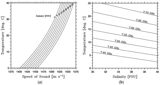
Figure 1.
The dependence of speed of sound (a) and Brillouin wavenumber shift (b) as a function of salinity and temperature. Panel (a) shows individual temperature versus speed of sound relationship over a range of practical salinity (PSU, 0–40 g/kg), with pressure set to a constant 0.0, and is adapted from Figure 2 in [39]. Panel (b) demonstrates the sensitivity of the Brillouin wavenumber shift over the expected range of ocean temperature and salinity values and is adapted from Figure 2 in [35].
In addition to the Brillouin wavenumber shift, a second feature of Brillouin scattering is the variability of the linewidth as a function of salinity, temperature, and pressure [41]. Several recent efforts have capitalized on using these two Brillouin scattering measurements, wavenumber shift and linewidth, to measure both temperature and salinity [42,43,44]. Meanwhile, another effort has demonstrated a multi-lidar technique to perform inversions using two wavenumber shift observations [45] to estimate both temperature and salinity.
Airborne lidars can retrieve data down to 3–4 optical depths, effectively allowing for profiling through the ocean thermocline in 70% of the ocean [46]. Such lidar systems have already been proposed for aircraft [17,36,46] and satellite [47] remote sensing applications to detect Brillouin scattering at depth. Theoretical estimates of ocean sound velocity profiles obtained using World Ocean Atlas 2018 data [48] and an empirical expression for sound velocity [49] compared well (difference 1–2 m/s) with direct laboratory measurements of Brillouin scattering using a benchtop lidar instrument in several studies [50,51]. Brillouin lidar instruments could potentially be developed for either ship-based, aircraft, or satellite to carry out large scale observations of the upper ocean thermal and salinity structures and mixed layer depths [17,47].
The advantage of using lidar technology to measure ocean temperature profiles over traditional methods such as ship-based CTD or profiling Argo floats, is that lidar measurements can be done rapidly from a ship, aircraft, or possibly a satellite. Lidar enables rapid measurement of sub-mesoscale features which has not been possible to date with either in situ, aircraft, or satellite technology. One disadvantage is that lidar instruments obtain point measurements of single profiles in time, which must be analyzed with consideration to their inability to obtain the larger scale synoptic scale measurements that are obtained by passive scanning satellite instruments such as AVHRR, MODIS, SeaWiFS, etc.
Using Brillouin lidar for measuring ocean temperature and salinity has been the topic of numerous studies, the majority of which have been instrument simulations. A lab study was carried out to demonstrate that Brillouin lidar can measure temperature profiles with a spatial resolution of 1 m and a mean accuracy of 0.07 deg. C [36], while another lab study demonstrated Brillouin lidar can retrieve sound velocity profiles with accuracy of 1–2 m/s [51]. Another instrument simulation study concluded that the detection of ocean MLDs using Brillouin lidar was feasible and reliable [17]. The expected global ocean variability of Brillouin lidar frequency shift was calculated using World Ocean Atlas 2018 data and a simulated Brillouin lidar [50]. And another simulated lidar study demonstrated the potential of obtaining optical profiles that extended deeper than the ocean MLD [47].
This paper presents results from several OSSEs that were carried out to quantify the capability of using a Brillouin lidar system to measure OHC and HSR. The OSSEs simulated the measurement of the ocean’s temperature fields with a Brillouin lidar in a Low Earth Orbit (LEO). Comparisons are made between the OHC and NHF calculated from the OSSEs with those obtained from an ocean circulation model. The correlation between the OSSEs and the model solutions are presented to demonstrate several measurement issues that would be encountered by an actual LEO instrument. The sections in the remainder of this manuscript include the following: a methods section that presents the numerical circulation model output used for the data set for the OSSE; the numerical calculations used to predict the probability of Brillouin lidar shot returns as a function of depth and ocean light attenuation coefficient; and, the OSSE technique for measuring the global ocean temperature profiles, upper ocean heat content, and heat storage rates using simulated LEO satellite trajectories. This is followed with a results section that presents the spatial and temporal variability of the observed OHS and NHF compared to the model solutions, and a discussion section that provides a summary of the results in the context of the needs for near-real-time ocean observations, and comments on potential observing solutions.
2. Materials and Methods
2.1. ECCO Model Solutions
The ECCOv4r4 model solutions were chosen as the ‘nature’ inputs for carrying out the OSSEs. Daily mean values of ocean potential temperature, , salinity, and MLDs were obtained from the Estimating the Circulation and Climate of the Ocean (ECCO) model, Version 4, Release 4, [52,53,54] (hereafter ECCOv4r4) run that simulated the global ocean from 1992 to 2017. The data were obtained from NASA’s PO-DAAC and made available after interpolation onto a uniform 0.5° resolution orthogonal grid [latitude bands: 89.75°S to 89.75°N; longitude bands: 179.75°W to 179.75°E] with 50 vertical grid levels that have higher resolution in the upper ocean domain. The model MLDs were also obtained at similar time and grid resolution.
The ECCOv4r4 model was developed to bring together a thorough set of heterogeneously sampled observations with a high-resolution ocean circulation model to serve as the data integration platform. ECCOv4r4 is a data assimilative model that makes use of ocean observations including sea level observed from satellite, global mean sea level, ocean temperature and salinity profiles obtained from CTDs, XBTs, Argo floats, glider, moorings, marine mammals, sea surface temperature, sea surface salinity, sea-ice concentration, ocean bottom temperature, and temperature/salinity climatology of the World Ocean Atlas 2009. See Table 2 in [53] for a complete list of observations used in the ECCOv4r4 solutions. The model solutions result in global predictions of temperature, salinity, velocities, etc. that are dynamically consistent with the often spatially and temporally under-sampled observations [53]. For instance, the resulting OHC from the ECCO model solutions compares well with the OHC analysis from various observational and reanalysis data (Figure 2), showing the long-term trends in the ocean’s energy imbalance.
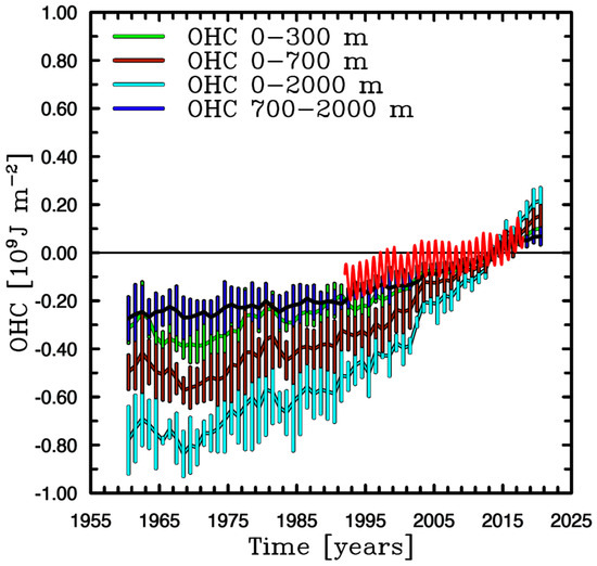
Figure 2.
A comparison of the ECCOv4r4 global 0–300 m Ocean Heat Content (OHC) anomalies (red curve) relative to the 2005–2020 climatology, calculated between 60°S and 60°N, with the resulting OHC anomalies [55] from the ensemble mean of various OHC analysis. Individual curves show the OHC anomalies obtained from integrating over various depth ranges (see figure legend). Vertical bars denote the 95% confidence interval (±2 standard deviations).
2.2. Ocean Mixed Layer Depths
One aspect of the OSSEs was to quantify the probability of measuring ocean temperature profiles down to the deepest observed MLD for a given region. Accurate real-time measurements of MLDs provide critical information on the upper ocean heat capacity necessary for improving hurricane forecasts [15]. In addition, temperature profiles obtained down to these depths can be used to calculate the upper ocean HSR. Previous work [28] has demonstrated that a threshold criteria temperature value of 1.0 °C provides the best isotherm for tracking the seasonal cycles of ocean HSR.
Two MLD climatology datasets [56,57,58] were obtained to calculate the spatially varying deepest MLDs at a 2° latitude × 2° longitude spatial resolution. The first MLD dataset [56] utilized nearly 4.5 million hydrographic profiles and a 0.2 °C temperature criterion to create a monthly mean MLD product. The second MLD dataset [57,58] was generated using more than 2.45 million Argo float profiles [10] with an improved hybrid algorithm rather than the standard threshold methods, resulting in more accurate and shallower MLDs. Even with different MLD depth selection criteria, the two MLD climatologies compared well with each other, with Pearson sample correlation coefficients (r) greater than 0.8 for nearly 70% of the MLD climatology’s. These two MLD climatology estimates were compared to the ECCOv4r4 MLD product, which uses a 0.8 °C temperature criterion for estimation of the MLDs [59,60]. The criteria values used for MLD determination studies using temperature- or density-based criteria varies between MLD studies (see Table 1 in [59] for a summary of the various T or density criteria).
Of the three MLD products, the MLD product obtained using Argo profiling floats data [57] was selected (Figure 3) for use in the Brillouin lidar return probability analysis presented below. The ECCOv4r4 MLD product showed much deeper winter MLDs in the North Atlantic and Southern Ocean areas than the actual MLD observations. The nature of the time varying climatologies of the MLD are not relevant for this study. Only the depth of the deepest MLD is required for setting the depths to which the temperature profiles were integrated for calculating the OHC and HSR.

Figure 3.
Deepest MLDs from the monthly mean gridded (2° latitude × 2° longitude) MLD climatology observed with the SIO Argo profiling floats using a 0.2 °C criterion [57].
2.3. Brillouin Lidar Signal to Noise Ratio (SNR) Calculations
The SNR analysis that was completed for this study was based on prior work on Brillouin scatter collection efficiency estimations [37]. The calculation for the strength of the return signal was estimated based on a modification of the basic link analysis equation that was modified for transmission through an optical medium with a different index of refraction:
where and are the number of detected and transmitted photons, is the Brillouin backscattering coefficient, is the range bin for collecting return signal and is the solid angle of the receiver, and are the efficiency of the detector and the optical system, and is the one-way transmission through the water. For this application the solid angle of the receiver, , is calculated in such a way to account for the index of refraction of the water medium such that
where is the area of the receiver, is the depth of penetration into the water, is the index of refraction of the water medium, and is the height of the receiver. The calculation of the transmission through the water was based on the input parameters for the attenuation coefficient (Kd) as well as the depth through the water. For simulation scenarios in which the receiver was positioned above the ocean surface an addition term for atmospheric transmission was provided as well to accurately account for losses of the optical path.
Atmospheric transmission as well as solar background was calculated by utilizing Py6s, which is a Python interface to the 6S radiative transfer model [61]. A solar elevation angle of 30°, an atmospheric profile of mid-latitude summer, and an aerosol profile of maritime were utilized for all transmission and solar radiation calculations. It was assumed for these calculations that the instrument of investigation was making a spectral analysis of the collected scatter light. This was done because of the previous work that has shown that water temperature and salinity can be calculated based on the measurement of Brillouin scatter peak separation as well as spectral width [62]. The collected scattered signal was assumed to be spectrally spread across a linear detector array that contained 32 elements and had spectral spacing of 1 p.m. A simulated Brillouin return spectrum was created with two gaussian peaks with Full Width at Half Maximum (FWHM) of 0.5 p.m. and a total separation between the two peaks of 16 p.m. This spectrum was then normalized by the total number of detected photons calculated in the return.
The strength of the signal for the SNR calculation was assumed to be the maximum value from this estimated spectrum. The SNR that was used in further calculations was estimated by the following equation [62]:
where is the calculated maximum number of detected photons from the estimated spectrum, is the estimated number of detected solar photons, and is the number of dark counts. For these estimates several assumptions were made for the instrument design. A 50 µJ, 532 nm, 100 kHz laser transmitter as well as a receiver telescope with a diameter of 0.3 m was utilized for the ocean surface return calculations. For LEO calculations, the laser energy was increased by a factor of 10 and the receiver aperture was increased by a factor of 4. The receiver system was estimated to have a quantum efficiency of 0.4 and a dark count rate of 20 kHz.
Signal to Noise Ratios (SNR) were calculated for a broad range of ocean attenuation levels ranging from 1.0 × 10⁻⁴ to 0.5 m−1 and for depths ranging from 1 to 349 m, at 1 m intervals. A laser pulse frequency of 100 kHz was used and SNR calculations were carried out with the laser situated at the ocean surface (0 m) and at LEO altitudes (400 km). The SNR levels ranged from 1.63 × 10+4 to 9.8 × 10−148 for the surface ocean calculations (Figure 4a), and 5.97 × 10⁻³ to 8.4 × 10−154 for the LEO calculations (Figure 4b). These SNR calculated values were extrapolated down to 1000 m depth by linear extrapolation of the Log10(SNR) values from the deepest calculated levels (349 m). The Log10(SNR) values are highly linear at ocean levels greater than 100 m.

Figure 4.
SNR (Log10) levels from one second integration of a 100 kHz Brillouin lidar operated at the (a) ocean surface and (b) LEO altitudes (400 km) for a range of light attenuation levels [m−1] and ocean depths [m].
2.4. Lidar Return Probability, and Standard Error Calculations
Lidar return probabilities () for lidar shots were calculated using the SNR results according to [63], such that
where is the number of individual lidar shots, and is the Threshold to Noise Ratio of the lidar, which for this study was set to 3, and is the ‘error function’. The simulations in this study used a lidar pulse frequency of 100 kHz and an integration time of 1 s. The levels of range from 0 to 1 for the surface ocean calculations (Figure 5a), and 0.0 to 0.9 for the LEO calculations (Figure 5b).
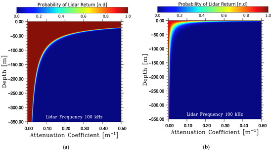
Figure 5.
Lidar Return Probabilities (LRP) for a one second integration of a 100 kHz lidar operated at the (a) ocean surface and at (b) LEO altitudes (400 km).
The parameter errors calculated for the lidar instrument were shown to be a function of the SNR values for both temperature and salinity. The errors were fitted to a power function and that equation was used to calculate the expected Standard Error (SE) from a one second integration of a 100 kHz instrument such that the
where is the value of the parameter error, are the total number of lidar shots. The plotted SE values (Figure 6) are masked to exclude regions where SE values that were higher than 1.5 deg. C, which is a reasonable level of instrument error of 1.0–1.5. Lower errors are possible by increasing the integration time of the measurement. However, note that these errors are derived from model estimates of the instrument error; these are simulated errors.
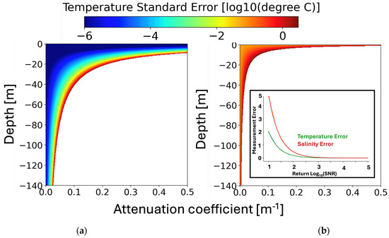
Figure 6.
Standard Error (%) for temperature at 0 m (a) and LEO (b) for a one second integration of a 100 kHz Brillouin lidar. Errors greater than 1.5 deg. C are masked to denote regions where observations cannot yet be retrieved with sufficient accuracy. The calculated errors as a function of the SNR for both salinity and temperature are shown as the inset figure in (b).
2.5. Global Ocean Diffuse Attenuation Coefficients at 490 nm
The 2020 annual mean diffuse attenuation coefficient, Kd(λ = 490nm), was obtained from the NASA/GSFC Ocean Biology Processing Group archive (Figure 7) and used in the Brillouin lidar OSSEs to estimate the LRP for specific regions in the global ocean. The data were used with an SNR lookup table (see Section 2.3), where SNR values varied as a function of attenuation coefficient (m−1) and depth [m]. Using the diffuse attenuation coefficient rather than an estimate of the beam attenuation coefficient is appropriate for the instrument design used in this study. The “effective” attenuation of the lidar system in ocean water approaches that of the diffuse attenuation coefficient when the instrument has a wide field of view for the receiver [37,64]. It should be noted also that multiple scattering should not be an issue since Brillouin scattering features are inelastic events that are dominated by singular events. The use of return spectra to determine Brillouin scattering features (temperature, salinity, speed of sound) is possible under multiple scattering because Brillouin scattering is limited to single scattering events [65]. In addition, the use of Kd estimates at λ = 490 nm for a lidar instrument with a laser wavelength of 532 nm is appropriate as Kd spectra tend to be flat or show a minimum region in that region of the visible spectra [66].

Figure 7.
The 2020 annual mean global ocean diffuse attenuation coefficient at 490 nm (Kd(λ = 490), m−1), obtained from the MODIS-Aqua satellite.
2.6. OSSE Satellite Simulations
Daily outputs of the full 3D mean temperature and salinity values from the ECCOv4r4 model solutions spanning from 1992 to 2017 (26 years) were used as the ‘nature’ component for the OSSEs. A simple Low Earth Orbit (LEO) for a satellite was simulated with a 60° inclination. Standard orbital equations for calculating the latitude (lat, [deg.]) and longitude (lon, [deg.]) positions of the satellite were employed such that,
where and are the satellite’s and Earth’s orbital periods [s], respectively, and are the initial and the independent variable, time [s], respectively, and is the satellite’s orbit inclination [rad.]. The values used in this study are given in Table 1.

Table 1.
The values used to calculate the simulated satellite trajectory as a function of time, t [s].
The trajectory of the simulated LEO satellite detailed above was used in all the OSSE experiments. These types of trajectories typically sample less over equatorial regions (Figure 8) due to the peak in its meridional speed as it crosses over the equator. As the satellite travels past the extremes in its latitudinal range its track becomes more zonal, resulting in a higher number of possible observations at the zonal extremes of its orbit. Using simulated satellite trajectories in the OSSE experiments provides information on how the sampling strategy, in this case a satellite orbit, impacts measuring ocean HSRs. Measuring the errors from the sampling strategies gives a relative sense to the additional errors caused by the Brillouin lidar instrument’s limitations of sampling the ocean temperature field. Sampling strategies and measurement technologies are both sources of error for remote ocean measurements.

Figure 8.
Bitmap plot of the shot count for a month of flight of a simulated satellite on a trajectory defined by Equations (7)–(11) and coefficients in Table 1, with a 1 Hz shot frequency. Binning occurred on a 1° longitude by 1° latitude grid. A single day trajectory is shown as a thick black curve.
2.7. Brillouin Lidar Mixed Layer Depth Measurement Probabilities
The Brillouin lidar probability solutions (Section 2.3) were used as a lookup table with the MODIS-A 2020 annual mean global ocean diffuse attenuation coefficient, Kd(λ = 490) (Section 2.3) to calculate the probability of a return Brillouin lidar signal as a function of geolocation and depth. These return probability profiles were compared with the calculated deepest MLD values obtained from the SIO Argo float data set (Section 2.2) to determine the probability of a lidar return signal from the deepest MLD being observable throughout the year for various ocean locations and for two different OSSEs, one a ship-mounted and the other a LEO satellite instrument. Note that the ship-mounted OSSE samples the ocean along the same trajectory as the LEO satellite. While this is not realistic, the solutions suggested by it demonstrate the impact of observing at LEO without an atmosphere.
2.8. Ocean Heat Content (OHC) and Heat Storage Rates (HSR) Calculations
The OSSEs were carried out by sampling the daily temperature and salinity fields from the ECCOv4r4 data set (Section 2.1) along the time/space trajectory of the simulated Brillouin lidar satellite (Section 2.6) from 1992 through 2017. The time step for the OSSE was set to 1 s, which coincided with the solutions from the Brillouin lidar probability calculations (Section 2.3). The observed temperature and salinity profiles were binned into 2° longitude by 2° latitude and 5° longitude by 5° latitude grids for the heat storage rate (HSR) calculations.
Ocean Heat Content (OHC) is the measure of the total amount of heat contained within a volume of ocean water, while the Heat Storage Rate (HSR) is the time rate of change of the OHC. The OHC and HSR calculations followed the method outlined in [21], such that the
where is the specific heat of seawater, h is the depth of integration, is the density of seawater, and is the mothly mean temperature. Unlike [21], where the depth of integration was chosen to track the depth of an isotherm located just below the winter mixed layer, the integration depth, , for this study was set as a constant value. This allows for characterizing the capability of the HSR results obtained by depth-limited measuring devices, such as a Brillouin lidar, to the HSR obtained from full or partial integrations of the water column’s temperature field. It should be noted that the experiments present results related to estimating the ocean HSRs rather than OHC. Estimating ocean HSRs is the more difficult and is more prone to errors that the more direct OHC measurements. The results focus on presenting the ability of a Brillouin lidar instrument to measure this more difficult, and error prone heat estimate.
Several ‘Nature’ and OSSE experiments were carried out to provide comparisons between the sampling strategies, measurement strategies and instrument measurement capabilities (Table 2). The first experiment (No. 1) estimated the HSR from the model by integrating the daily individual temperature fields to the bottom of the ocean model using the gridded 0.5° longitude by 0.5° latitude grid. This first experiment will be referred to in this paper as a baseline solution, against which the other experiments are compared. A series of three additional ‘Nature’ experiments were carried out by altering the depth to which the temperature profiles were integrated to estimate the HSRs. Experiments 2–4 used integration depths that were set by the (No. 2) depth of the deepest SIO Argo MLD, (No. 3) ECCO model deepest MLD, and (No. 4) ECCO model deepest climatology mean plus 2 standard deviations MLD. All these experiments sampled the ECCO temperature fields by directly measuring each of the available daily model output fields. The daily temperature field were binned into monthly mean temperature fields at both 2° longitude by 2° latitude and 2° longitude by 2° latitude grids from which monthly mean HSRs fields were calculated. Similar monthly binning, gridding and finite differencing was carried out on all experiments to calculate OHC and HSRs.
Table 2.
List of various HSR ‘Nature’ or OSSE experiments.
A series of four OSSE experiments (Nos. 5–8) were carried out to compare the impact of sampling the model solutions by using the trajectory of the simulated satellite trajectory to sample over time and space. In these experiments it was assumed that the satellite was able to measure the full top to bottom temperature profile of the model every second over the 1992–2017 period of the model solutions. So, while the Nature experiments were able to sample all the 3D model’s temperature fields, the OSSE experiments were limited by the simulated satellite’s trajectory.
Finally, two OSSE experiments (Nos. 9 and 10) were carried out to investigate the impact of using a Brillouin lidar instrument to measure ocean temperature profiles. The probability solutions were estimated for a Brillouin lidar instrument operated at the ocean surface (No. 9) and at a LEO elevation (No. 10). These simulations make use of the probability lookup tables (Section 2.3) and the 2020 annual mean global ocean diffuse attenuation coefficients, Kd(λ = 490 nm) (Section 2.4). Note that it is not feasible to measure ocean’s temperature fields such as was carried out in experiments 1–9, only experiment 10 is a near realistic estimate of a possible observing strategy for a Brillouin lidar instrument. Experiments 1–9 provide a baseline for understanding the errors encountered in developing such an observing system. All the solutions to the experiments were binned using both a 2° longitude by 2° latitude and 5° longitude by 5° latitude grids.
All of the Fortran software used for simulation, analysis and creating figures is available for download as Supplementary Materials per NASA’s Open Science Policy.
3. Results
The results below present information from this study that are framed to shed light onto the various issues that were encountered in simulating a Brillouin lidar instrument for operation at LEO. Both SNR degradation from operating the Brillouin lidar at increased elevations (ocean surface vs. LEO) and errors obtained from sampling along a LEO orbit reduced the ability to correctly monitor the HSR of the ocean at a monthly time scale. The results from analysis of various components of this measurement system are presented below.
3.1. Probability of Profiling to Mixed Layer Depth Measurements
Global maps of the probability of lidar returns from the MLD were calculated for the 0 m (Figure 9a) and LEO (Figure 9b) deployment scenarious using the SNRs for the two operation solutions (Section 2.4), the mean 2020 MODIS-A diffuse attenuation coefficient (Section 2.5) and the MLDs from the SIO Argo MLD climatology (Section 2.2). Low probabilities are observed in both cases in regions where the MLDs are deepest, such as in the Southern Ocean and North Atlantic (Figure 5). But for the LEO estimates, low values occur as a result of both higher light attenuation and deeper MLDs. The dramatic shift into lower lidar returns for most of the ocean is a significant source of errors in the resulting HSR estimates.
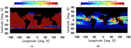
Figure 9.
The lidar return probability (LRP) of a Brillouin lidar return signal from the observed SIO Argo deepest climatology mixed layer depth from the simulated Brillouin lidar instrument operated at the ocean surface (a) and at LEO (b).
3.2. ‘Nature’ and OSSE Solutions: ECCOv4r4 Heat Storage Rates (HSRs)
3.2.1. HSR from Integration to the ECCO Ocean Bottom
Daily, monthly, and long term mean OHC fields were calculated by integration of the ECCO temperature profiles down to the model’s deepest level. The long term mean OHC (Figure 10) shows the influence that the ocean’s variable bathymetry has on the OHC fields, deeper waters contain more heat. For instance, the shallowing along the mid-ocean ridges, the 90-degree line in the Indian Ocean, and along the Philippine Sea Plate region in the western Pacific all show lower levels of OHC from the shallower depths. This spatial variability does not create errors in the Nature HSR calculations because the bathymetry in each grid cell remains constant. But in the OSSE that integrated the temperature to the bottom of the ocean, binning the integrated profiles of temperature obtained along the satellite trajectory introduces errors by sampling in ocean areas that have different depths. Because of this, the Nature experiment (No. 1) that calculated the HSRs by integration to the ocean bottom was used in this study for comparison against the various Nature and OSSE experiments.

Figure 10.
The mean (1992–2017) Ocean Heat Content (OHC) obtained by integrating the ECCOv4r4 daily outputs of temperature at a 0.5° longitude by 0.5° latitude resolution grid from the surface to the model’s ocean bottom.
3.2.2. HSRs from Integration to the SIO Argo Deepest MLD
Monthly mean HSRs were obtained at both the 2.0° × 2.0° and 5.0° × 5.0° spatial resolution by integrating the sampled ECCO temperature profiles down to the deepest depths observed MLD in the SIO Argo MLD climatology. On a global scale, both the Nature- and OSSE-derived HSR fields showed the expected distribution of values at both the 5.0° × 5.0° (Figure 11a; panels A & B) and 2.0° × 2.0° (Figure 11b; panels A & B) averaging scales. The large-scale zonal distributions agree with expectations regarding the global seasonal ocean heating, with large positive values in ocean areas influenced by expected seasonal heating co-varying with the large negative values in areas under cooling conditions. Few notable anomalous regions are noted in either the Nature or OSSE solutions. However, the OSSE 2.0° × 2.0° resolution solutions (Figure 11b, panel B) show obvious errors due to the satellite track causing under-sampling of the ocean temperature fields. Under-sampling of the ocean remains an issue for all of ocean science. In a previous a study it was found that estimates of HSR at 5.0° × 5.0° resolution provide the optimal HSR solutions, with the least impact from errors due to mesoscale variability [21]. Because of this, and the noted under-sampling, the results presented below focus on the 5.0° × 5.0° resolution grid solutions.
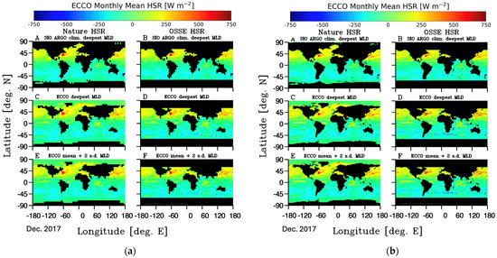
Figure 11.
The July 2017 monthly mean Heat Storage Rates (HSR) obtained from integration of the ECCO daily temperature fields down to the SIO ARGO deepest climatology MLD (A,B), the ECCO mean MLD (C,D), and the ECCO mean + 2 standard deviations MLD (E,F) for the ‘Nature’ (A,C,F) and OSSE (B,D,F) calculations using the (a) 5° longitude by 5° latitude and (b) 2° longitude by 2° latitude resolution binning solutions. The small red points off the eastern U.S. denote the location from where the time series of results (Figure 12) was obtained. All monthly images are available for download as Supplementary Materials.
3.2.3. HSR from Integration to the ECCO Deepest MLD
Monthly mean HSRs were calculated at both the 2.0° × 2.0° and 5.0° × 5.0° spatial resolution by integrating the ECCO temperature profiles down to the deepest MLD from the ECCO model. Both the ‘Nature’- and OSSE-derived HSRs showed spatial patterns like the SIO Argo MLD integrated solutions, at both 5.0° × 5.0° (Figure 11a; panels C & D) and 2.0° × 2.0° (Figure 11b; panels C & D) resolution grids. The map of the monthly mean HSRs showed regions of increased HSR variability in the North Atlantic and North Pacific Western Boundary Currents and in the Southern Ocean frontal regions, all regions of increased mesoscale activity, sharp thermal fronts, and deeper mixed layers.
3.2.4. HSR from Integration to the ECCO Deepest Mean + 2 std. dev. MLD Climatology
The final set of HSR calculations integrated the ECCO temperature profiles down to the deepest climatology mean plus 2 standard deviations of the ECCO MLD. HSR calculations were carried out by binning at both 5.0° × 5.0° (Figure 11a; panels E & F) and 2.0° × 2.0° (Figure 11b; panels E & F) resolution grids. While the depths for integration in these calculations was deeper than the SIO Argo and ECCO deepest MLD, the solutions showed strong agreements with the ECCO HSR solutions from integrating to the ocean bottom.
3.2.5. HSR Time Series Comparisons and Global Correlations
A comparison of the HSR time series from the grid cell representing 35°N to 37°N and 60°W to 62°W (See Figure 11 for red-dot locations) shows that the time series of the three ‘Nature’ experiments (No. 2–4) that integrated the temperature profiles to different ocean depths compare very well at that ocean location with the ‘Nature’ experiment (No. 1) that integrated the temperature profiles to the ocean bottom (Figure 12a). A similar strong correlation is observed when comparing the time series of the three OSSE experiments for that same region (Figure 12b).

Figure 12.
The monthly mean HSR (1997–2017) for the various (a) Nature experiments which calculated the HSR by integrating temperature profiles down to the ARGO deepest MLD climatology (blue curve), the ECCO deepest MLD (green), the ECCO mean + 2 standard deviations MLD (red), and the model bottom (black), and (b) OSSE experiments which calculated the HSR by integrating temperature profiles down to the ARGO deepest MLD climatology (blue curve), the ECCO mean MLD (black) and ECCO mean + 2 standard deviations MLD (red).
The strength of the correlations between the baseline ‘Nature’ experiment (No. 1) and those of the three Nature (Nos. 2–5) and the three OSSE experiments (Nos. 6–8) varies with ocean regions (Figure 13). Regions of high correlation appear in zonal midlatitude bands, with lower correlations in the low-latitude regions near the equator for the SIO Argo MLD (No. 2 and 6), likely due to the Argo MLD being too shallow to capture thermal structures below the equatorial region that seem to be captured by the experiments that integrated the temperature profiles based on the ECCO MLDs. In addition, there are areas in the equatorial region of the Argo MLD integrated experiments where the correlations are below the threshold of significance, as determined by the t-test on the Pearson Correlation coefficients. The low correlations at low latitudes correspond to the high variability in the OHC due to the equatorial waveguide and the westward propagating Rossby waves, which are constant and prominent features in the ECCO model solutions. For those experiments that used the ECCO MLD fields to calculate the HSRs, there exists two zonal areas of low correlation in the regions just to the north and south of the equator and where the main thermocline has the highest spatial variability due to its doming to shallow levels near the equator.

Figure 13.
The Nature HSRs calculated by integrating to the bottom of the ocean model (Experiment No. 1) and the various Nature and OSSE HSR experiments (Experiments 2–7). Shown are HSR correlations for (A,B) Experiment 1 vs. 2 and 5, for the Nature (A) and OSSE (B) experiments that integrate to the SIO ARGO deepest climatology MLD, (C,D) Experiment 1 vs. 3 and 6, for the Nature (C) and OSSE (D) experiments integrating to the ECCO deepest MLD, and (E,F) Experiment 1 vs. 3 and 7, for the Nature (D) and OSSE (F) experiments integrating to the ECCO mean + 2 standard deviations MLD. The left side panels are the results for the ‘Nature’ (A,C,F) and right-side panels are for the OSSE (B,D,F) calculations. The solutions are carried out using 5° longitude by 5° latitude. Correlations that fail the student t-test (t < t0.5(2),298 = 1.968) are colored in olive.
Comparing the level to which each of these Nature and OSSE solutions (Nos. 2–4, and Nos. 6–8) correlate to the baseline ‘Nature’ experiment (No. 1) provides a clear understanding of how satellite sampling errors can impact the HSR solutions. Also, it is noteworthy that for most of the mid-latitude regions the correlations are strong with much (38–50%) of the ocean regions having correlations above 0.8. While the Argo MLD integration solutions showed lower correlations near the equatorial regions, the solutions had the largest pixel number (>50%) with greater than 0.8 correlation values. In addition, the HSRs for the three Nature and OSSE experiments that integrated the sampled temperatures profiles using different MLD choices (Figure 14) showed very strong correlations, with the best from the SIO Argo MLD solutions. This observed strong correlation between the Nature and OSSE HSR solutions was why the SIO Argo depth integration criteria was chosen for the two Brillouin lidar OSSEs whose results are presented below. The choice of the depth integration criteria had a significant impact on the accuracy of the HSR solutions, with the SIO Argo MLD criteria yielding the best HSR solutions relative to the Nature base experiment.
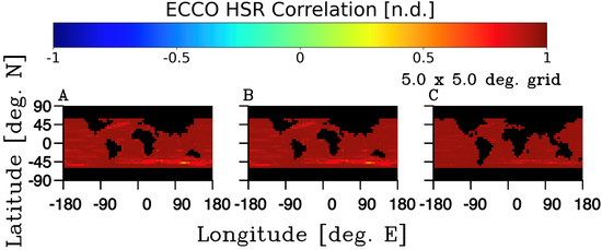
Figure 14.
Correlation of the Nature vs. OSSE calculations from integrating the temperature fields using the same integration depth selection. Results shown are for integrating to (A) the ECCO deepest MLD, (B) the ECCO deepest climatology + 2 s.d. MLD, and (C) the SIO ARGO climatology deepest MLD. These correlations reflect comparisons from the experiments outline in Table 2 for (A) experiments 3 vs. 7, (B) experiments 4 vs. 8, and (C) experiments 2 vs. 6.
3.3. OSSE: Brillouin Lidar Heat Storage Rate (HSR)
3.3.1. Brillouin Lidar OSSE Flown at 0 m (Ocean Surface) with HSR Integration to SIO Argo Deepest MLD
The resulting HSR fields obtained by incorporating the Brillouin lidar instrument return probabilities calculated for an altitude of 0 m (Figure 5a) with the SIO Argo deepest MLDs for temperature profile integration depth criteria (Experiment No. 9) provided a solution that demonstrated how the optical conditions of the ocean impact the resulting HSRs. This experiment does not contain errors that would result from deploying the Brillouin lidar instrument at higher elevations nor from the influence of an atmosphere. They are a useful for understanding the impact of the ocean’s optical properties on the resulting HSRs, especially considering the satellite track sampling errors already demonstrated in the earlier sections.
Overall, the monthly mean HSRs for this 0 m Brillouin lidar OSSE (Figure 15A) agree well with the Nature and OSSE experiments (Nos. 2 and 6) that also used the SIO Argo MLDs for the integration criteria (Figure 15C,D). In these latter two experiments, the probability of measuring the temperature profile was 1. What is noticeable in comparing these three solutions is that the Brillouin lidar OSSE has anomalously high and low HSRs in regions of low lidar return probability for this 0 m deployment case (Figure 9a), such as the region along the Southern Ocean, and several points in the North Atlantic.
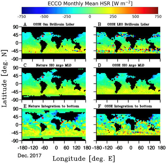
Figure 15.
December 2017 monthly mean HSR from the (A) Brillouin lidar OSSE flown at 0 m using the SIO Argo MLD integration criteria, (B) Brillouin lidar OSSE flown at LEO using the SIO Argo MLD integration criteria, (C) Nature solution using the SIO Argo MLD integration criteria, (D) OSSE solution with SIO Argo MLD integration criteria, (E) Nature experiment with integration to the bottom, and (F) OSSE with integration to the bottom. The small red points off the eastern U.S. denote the location from where the time series of results (Figure 16) was obtained. All monthly images are available for download as Supplementary Materials.
The HSR time series of the 0 m Brillouin lidar OSSE (Figure 16, red curve) from the grid cell representing 35°N to 37°N and 60°W to 62°W (See Figure 15 for red-dot locations) compares well with the baseline Nature experiment (Exp. No. 1, Figure 16, black curve). The direct comparison between the baseline Nature (Exp. No. 1) and the 0 m Brillouin lidar OSSE HSR solutions shows strong agreement. This is encouraging when considering the capability and observing potentials of deploying a Brillouin lidar instrument from a ship or low-flying aircraft.

Figure 16.
The monthly mean time series (1997–2017) of the Nature HSR calculations that integrated the temperature profiles to the bottom of the model (black) and the OSSE calculations that integrated down to the SIO ARGO deepest MLD and flown at 0 m (red) and LEO (blue).
The correlation between the Nature and OSSE HSR estimates that used the SIO Argo MLD integration criteria (Exp. Nos. 2 and 6, Figure 17A) is very high for all regions of the ocean, with lower correlations occurring those regions of ocean mesoscale variability, such as along the Southern Ocean frontal region. These are also regions that contain lower lidar return probabilities (Figure 8). Lower lidar return probabilities reduce the number of observations which elevates the uncertainty in the HSR solutions. These ocean regions are where there are elevated levels of mean diffuse light attenuation, as estimated from the MODIS-A Kd(λ = 490) field (Figure 6), which further reduces the probability of a lidar return.

Figure 17.
Correlation of the Nature vs. OSSE calculations that integrated the temperature fields down to the SIO ARGO climatology deepest MLD for (A) experiments 2 vs. 6, (B) experiments 2 vs. 9, and (C) experiments 2 vs. 10. These correlations compare the OSSE experiments that sampled the temperature profiles with a sampling probability profile of (A) 1, (B) determined using the Brillouin lidar return probabilities for operations at the ocean surface (0 m), and (C) determined using the Brillouin lidar return probabilities for operations at LEO (400 km). When possible, all measured temperature profiles were integrated down to the SIO ARGO deepest climatology MLD.
In comparison, the correlations between the Nature and 0 m Brillouin OSSE, also using the SIO Argo MLD integration criteria (Exp. Nos. 2 and 9, Figure 17B) show that the reduction in the correlations again occurs primarily in those regions that contain lower lidar return probabilities (Figure 8). These areas of lower correlation cover a much larger ocean region. These results demonstrate the impact of the reduction in lidar return probabilities on the HSR estimates and the influence deep mixed layer regions have on the capability of obtaining ocean temperature profiles using a Brillouin lidar. Strong declines in the correlations are observed in the Southern Ocean and along the western boundary current region of the North Atlantic, where deeper mixed layers are observed.
3.3.2. OHC Brillouin Lidar Flown at LEO with HSRs from Integration to SIO Argo Deepest MLD
The final OSSE experiment (No. 10) obtained HSR estimates from simulating a Brillouin lidar flown in a LEO satellite simulation at the elevation of 400 km. This experiment’s probability of lidar return was impacted by the inclusion of an atmospheric layer in the calculation of the SNR values (Figure 4b) which significantly decreased the probability of light pulse returns as a function of depth and light attenuation in the ocean (Figure 5b). It is because of this that the solutions to the HSRs show regions with high levels of noise (Figure 15B). Overall, the bitmap of daily HSR shows good agreement with the Nature and OSSE experiments that did not estimate the HSR by integration to the ocean bottom but rather integrated through an upper ocean layer, such as some determined MLD field. The HSR time series of the LEO Brillouin lidar OSSE (Figure 16, blue curve) from the grid cell representing 35°N to 37°N and 60°W to 62°W (See Figure 15 for red-dot locations) compares very well with the baseline Nature experiment (Exp. No. 1, Figure 15, black curve). That the direct comparison between the baseline Nature (Exp. No. 1) and the LEO HSR time series compares well even with the addition of an atmospheric layer shows the level of promise that this technology has for fielding as a satellite instrument. There are several points of time where the LEO Brillouin lidar simulation shows a mismatch with the Nature experiment. All these mismatches appear as a set of large positive and negative anomaly pairs, which suggests a single time point error in the OHC calculation impacting the time derivative HSRs.
3.4. Comparison of OSSE Brillouin Lidar Flights with Other HSR Calculations
The correlations between the various Nature and OSSE experiments are useful for demonstrating the level of spatial agreements between the experiments. One such correlation between the Nature and the OSSE experiments that integrated the temperature profiles down to the SIO Argo MLDs (Figure 14C and shown again in Figure 17A for direct comparison) showed that the fixed versus satellite track sampling techniques produce comparable HSR solutions. For the Brillouin lidar 0 m flight simulation (Figure 17B), the regions where the correlations drop coincides with regions of deep MLDs (Figure 3). When the Brillouin lidar simulation is performed with a LEO satellite (Exp. 10), the HSR correlations with the Nature experiment decreased significantly (Figure 17C). The regions of reduced correlation coincide with regions of deep MLDs and increased light attenuation (Figure 7).
A comparison of the histograms of the Coefficient of Determination (r2) obtained by correlations between the various Nature and OSSE HSR experiments (see Figure 13 as an example) provides a summary of the two main sources of errors in estimating the HSRs with a space-based Brillouin lidar instrument (Figure 18). The histograms obtained by correlating the baseline Nature calculation (Exp. No. 1) with each of the other Nature and OSSE experiments (Exp. Nos. 2–10) shows the difficulty in obtaining high correlations between the fully integrated water column HSRs and other estimation methods that sample using both a grid or a satellite flight track, and a variety of depth-integration criteria (Figure 18a). In fact, the Brillouin lidar LEO HSRs (Figure 18a, I) shows very poor histogram of correlations.

Figure 18.
Histograms of the coefficient of determination (r2) for the various Nature and OSSE HSR experiments (Exp. Nos. 2–10) correlated with (a) the Nature baseline experiment (Exp. No. 1) and (b) the Nature experiment using the SIO Argo MLD integration depth criteria (Exp. No. 2).
Correlations between the Nature calculation that used the SIO Argo deepest MLD integration criteria (Exp. No. 2) and the other HSR Nature and OSSE calculations show a significant improvement in their level of skill (Figure 18b). The histograms of the correlations between the Nature HSR calculations that used different MLD fields to integrate down to (Exp. Nos.: 2 vs. 3, and 2 vs. 4) demonstrate that the surface HSRs do not vary greatly by changing the MLD integration criteria. More important is that correlations between the Nature and OSSE experiments with MLD integration criteria showed high levels of correlation (Figure 16). As an example, the histogram between the Nature and OSSE HSR calculations that used the SIO Argo deepest MLD integration criteria (Figure 17A; Exp. Nos. 2 vs. 6) show very good agreement (Figure 18b, E). These strong correlations are only slightly diminished in the Brillouin lidar 0 m flight probability calculations (Figure 17B, Figure 18b, H). For the Brillouin lidar LEO flight probability calculations the histogram of the correlations (Figure 17C) is reduced because of the significant loss in retrieval probabilities rather than inability to measure the HSRs, which yielded a bi-modal distributions in the histogram (Figure 18b, I). Presently, low to mid-latitude ocean regions are likely areas where a space-based Brillouin lidar instrument can retrieve adequate measurements to obtain profiles of ocean temperature.
4. Discussion
Observing the ocean temperature fields, even with perfect instrumentation for measuring temperature profiles to the ocean bottom, introduces errors through the way the observations are collected in time and space. For point-wise remote-sensing instruments, such as a laser instrument that is limited in its observing a singular ocean spot, as opposed to a swath or image, these errors can be significant impediments to an observing system. This research used numerical ‘Nature’ calculations and OSSEs to calculate monthly mean maps of the OHC and HSRs. These are difficult measurements to make and are traditionally calculated using coupled ocean-atmosphere models [55,67], altimeter observations smoothed over long time and space scales [68], or through tedious analysis of the available in situ measurements [69,70]. Even with the present high number (~4 K) of profiling Argo floats providing more than 100 K of ocean temperature profiles each year, estimating the OHC and HSR remains a challenge because of the sparseness and irregular coverage in the collected data [55]. This paper used the challenge of making OHC and HSR observations to assess the limitations that a Brillouin lidar instrument would need to overcome.
A main result in this study is that the Brillouin lidar satellite sampling strategies are significantly impacted by spatially varying ocean features (MLDs, diffuse attenuation) which alter the ability to obtain quality observations for measuring OHC and HSR. These differences are demonstrated by the histogram of the correlations between the HSR time series from the Nature and OSSE experiments, both of which use full surface to ocean bottom temperatures (Figure 18). Even a hypothetical instrument capable of measuring the entire ocean temperature profile would encounter errors by measuring along the track of a satellite’s orbit. This is mainly due to the limited ability to obtain a good estimate of the mean temperature profiles from the sparse measurements obtained within the highly dynamic ocean. The introduction of flight-induced bias is well-known [71]. It is likely that these types of observational errors can be minimized by developing an error-reducing strategy that considers the time and location of the observations within the grid to which the observations are being averaged over.
The second result from this study confirms that estimates of the upper ocean’s OHC and HSR fields are resilient regardless of the selected integration depth criteria. The correlations between the various Nature and OSSE solutions were high between any of the experiments, Nature or OSSEs, that did not integrate down to the ocean bottom (examples are shown in Figure 14; Figure 18a, panels B, C, D). This result also provides further support to the paper’s first findings regarding the sampling bias errors.
While it is encouraging that the second result shows the resilience of using upper ocean temperature observations for OHC and HSRs, there is still a need for developing a methodology that can use upper ocean measurements to assess the entire water column’s heat content.
The third result from this study is that a surface deployed Brillouin lidar instrument can observe the upper ocean temperature profiles adequately enough to estimate OHC and HSRs. While the operation of a satellite at the ocean surface is not possible, deploying such as lidar instrument from a ship or a low-flying aircraft is. Deployments from a ship could serve to make automated temperature profiles such as those that have been carried out for nearly 55 years [72] using eXpendable BathyThermograph (XBTs). Repeat transects of subsurface temperature profiles have been applied for a wide range of upper ocean studies, such as estimates of western boundary currents [73] and have shown that weekly subsurface temperature measurements have a large impact on simulating the mean and subsurface circulation fields. Other studies have shown their importance in estimating circulation patterns and heat content in dynamic western boundary current regions [74] and improve model predictions when available for assimilation into regional ocean circulation models [75]. Deployment of Brillouin lidar instruments on ships of opportunity and possibly to replace or augment the XBT repeat survey lines would greatly increase the number of temperature and salinity observations in the upper ocean at a time when accurate global ocean temperature predictions are critical.
Deployments on a low flying aircraft or Unmanned Airborne Vehicle (UAV) could support oceanographic field surveys that target important physical processes such as mapping of the thermal and density structure of sub-mesoscale features along a frontal zone or eddies. These types of process studies are presently out of reach for many physical oceanographers who continue to wrestle to understand the rapidly evolving sub-mesoscale features using information obtained from slow moving profiling glider, floats, and research vessels.
While the results show that a Brillouin lidar flown at LEO can observe the evolving OHC in the upper ocean for the lower to mid-latitude regions, it is the higher latitudinal ocean regions that require greater observing because those regions play a significant role in controlling the Earth’s climate and weather patterns and are the most vulnerable in Earth’s present state of climate change. As the technology for Brillouin lidar will continue to develop and achieving those observations will become more feasible, there may be value in having a rough comparison of the costs and benefits of a dedicated LEO Brillouin lidar mission to the present Argo Program for observing the upper ocean temperature field. Assume that a 100 kHz Brillouin lidar instrument could collect one temperature/salinity profile per second and was deployed over a five-year flight mission. This would yield approximately 110 million observations (assuming 70% ocean hits but not accounting for clouds), which for a $1 billion mission would average $9/profile. Compare that estimate to the Argo Program [9] which profiles the upper 2000 m of the ocean with ~3000 profiling floats at the cost of ~$20 million per year to collect ~100 k profiles or $200 per profile. Beyond the need to improve the technology is the need to obtain the observations, which will require completion of OSSEs to assess the benefits and an evaluation by the ocean observing science community for assessing those findings.
Ocean regions with deep mixed layers and high light attenuation ocean water are areas that hold significant impediment to obtaining full upper ocean temperature and salinity profiles. It is those regions that poor HSR solutions were anticipated from the lidar return probability calculations. And those regions were where the HSR calculations failed (Figure 17C). The North Atlantic region is one specific region of interest that is impacted by both deep mixed layers and high light attenuation. It is a region where there is a need for obtaining accurate measurements of OHC and HSR measurements to assist in modeling and monitoring the AMOC, especially in terms of developing a possible early-warning indicator capability [14]. While it may be an area that remains out of reach for a satellite-deployed Brillouin lidar instrument, ship and/or aircraft-deployed instruments could obtain those observations if such a lidar instrument was ready for such use.
The OSSE retrievals in this study did not consider the impact of clouds on the retrievals of the Brillouin scattering signals. Clouds will be more of an issue along the equatorial regions and in the higher latitudes, where passive remote sensing retrievals are already difficult. Future OSSEs should consider taking this into account. Clouds will not impact any ship or likely aircraft deployed lidar systems.
While this Brillouin lidar technique for measuring ocean water features was proposed nearly a half century ago [30], a recent flurry of work [30,31,32,33,34,38,39,40,41,42,43,44,45] has been done on the ability of using Brillouin lidar to measure temperature, salinity, and sound speed. Various laboratories are developing benchtop instrumentation and testing the capability using select samples of ocean water. What is now required is for the laboratory benchtop systems to parameterize and confirm the capability of these benchtop instruments using a broad range of seawater samples with varying salinities, temperatures, and pressures. In addition, realistic models of the various Brillouin lidar instruments should be interfaced with ocean models to carry out additional OSSEs that can provide further evidence on the impact that these measurements can have of ocean modeling and predictions.
It is anticipated that Brillouin lidar technology will soon become available for deployment as an aircraft instrument for research and for possible ocean monitoring to aid in weather forecasting, for instance, tropical storms. That moment will likely open a new era into scientific observations on sub-mesoscale ocean features and processes, an aspect of ocean research that continues to elude ocean science even in this era of satellites and autonomous instruments.
Improving the use of Brillouin lidar measurements for OHC and HSR studies will requires additional OSSE experiments to quantify the errors in the measurement process and to include quantification of the errors introduced by the sampling strategy. In addition, OSSEs should be developed in such a way as to embed more realistic models of the lidar instruments, for instance, a digital twin. This study did not simulate the lidar instrument measurement errors, this will need to be done as the instrument becomes further developed. These new methods of developing simulations offer up a tremendous advantage to understanding instrument and measurement errors for any instrument in development and testing.
Supplementary Materials
In support of NASA’s Open-Source Science Initiative, the following information can be downloaded at: https://github.com/nasa (accessed on 8 March 2024): All fortran-90 programs used in preparation of the data, analysis, and creation of the figures.
Author Contributions
Conceptualization, J.R.M., C.S.R., G.B.C. and P.R.S.; methodology, J.R.M., G.B.C. and P.R.S.; software, G.B.C. and J.R.M.; validation, J.R.M. and G.B.C.; formal analysis, G.B.C., D.P.P. and J.R.M.; investigation, D.P.P., G.B.C. and J.R.M.; resources, C.S.R., P.R.S. and G.B.C.; data curation, J.R.M.; writing—original draft preparation, J.R.M.; writing—review and editing, C.S.R., G.B.C. and P.R.S.; visualization, J.R.M.; supervision, C.S.R.; project administration, C.S.R.; funding acquisition, C.S.R. All authors have read and agreed to the published version of the manuscript.
Funding
This research was funded by the NASA Goddard Space Flight Center’s Internal Research And Development (IRAD) Program to PI C. Rousseaux.
Data Availability Statement
The data used and presented in this study are openly available in the following various archives: ECCO Data: ECCO Version 4 Release 4 (R4) data [62] is available on NASA’s Physical Oceanography Distributed Active Archive Center (PO.DAAC). The complete set of daily mean fields on the ECCO Data Portal: https://archive.podaac.earthdata.nasa.gov/podaac-ops-cumulus-protected/-ECCO_L4_TEMP_SALINITY_05DEG_DAILY_V4R4/ and the complete set of daily MLD estimates are at: https://archive.podaac.earthdata.nasa.gov/podaac-ops-cumulus-protected/ECCO_L4_-MIXED_LAYER_DEPTH_LLC0090GRID_DAILY_V4R4/, Data Accessed: 1 September 2022. Global Ocean Heat Inventory Data: The global ocean heat inventory data [17] used for comparison with the ECCOv4r4 OHC (Figure 2 in [17]) was obtained from the World Data Center Climate data repository (http://www.lwdc-climate.de (accessed on 8 January 2024)), Identifier: doi:10.26050/WDCC/GCOS_-EHI_19602020_OHC, filename: GCOS_EHI_1960-2020_Earth_Heat_Inventory_Ocean_Heat_Content_data.nc. SIO Argo Data: The Argo program is part of the Global Ocean Observing System, and its data are made are freely available by the International Argo Program and the national programs that contribute to it. (https://argo.ucsd.edu, https://argo.jcommons.org). The Argo Program is part of the Global Ocean Observing System (doi.org/10.17882/42182#56126). The MLD dataset developed by [57] is made available at http://mixedlayer.ucsd.edu. The dataset of the MLD climatology at a 1° latitude × 1° longitude spatial resolution is updated periodically as more data becomes available. The Argo-derived MLD dataset for the data set used in this effort was dated 14 April 2022. IFREMER MLD Data: The MLD dataset developed by [56] is made available from https://cerweb.ifremer.fr/deboyer/mld/Surface_Mixed_Layer_Depth.php. The dataset of the MLD climatology at a 2° latitude × 2° longitude spatial resolution is contained in filename: mld_T02_c1m_reg2.0.nc, Data generation date: 4 November 2008, Data accessed: 13 March 2022. NASA MODIS-Aqua Global Ocean Diffuse Attenuation Coefficient Data: The 2020 annual mean diffuse attenuation coefficient at 490nm was obtained from the NASA/GSFC Ocean Biology Processing Group’s MODIS-Aqua Level-3 Standard Mapped Image archive. https://oceancolor.gsfc.nasa.gov/l3/. Observations are at a 1/12th degree (9 km) spatial resolution. Filename: A20200012020366.L3m_-YR_KD490_Kd_490_9km.nc Date created 22 February 2021.
Acknowledgments
Graphic capability was provided by the National Center for Atmospheric Research (NCAR) Graphics Package using GNU Fortran. The authors are grateful to the three reviewers for helpful comments and suggestions.
Conflicts of Interest
The authors declare no conflict of interest. The funders had no role in the design of the study; in the collection, analyses, or interpretation of data; in the writing of the manuscript; or in the decision to publish the results.
References
- Church, J.A.; White, N.J.; Konikow, L.F.; Dominques, C.M.; Cogley, J.G.; Rignot, E.; Gregory, J.M.; van den Broeke, M.R.; Monaghan, A.J.; Velicogna, I. Revisiting the Earth’s sea-level and energy budgets from 1961 to 2008. Geophys. Res. Lett. 2011, 38, L18601. [Google Scholar] [CrossRef]
- Levitus, S.; Antonov, J.I.; Boyer, T.P.; Baranova, O.K.; Garcia, H.E.; Locarnini, R.A.; Mishonov, A.V.; Reagan, J.R.; Seidov, D.; Yarosh, E.S.; et al. World ocean heat content and thermosteric sea level change (0–2000 m), 1955–2010. Geophys. Res. Lett. 2012, 23, L10603. [Google Scholar] [CrossRef]
- Seneviratne, S.I.; Zhang, X.; Adnan, M.; Badi, W.; Dereczynski, C.; Di Luca, A.; Ghosh, S.; Iskandar, I.; Kossin, J.; Lewis, S.; et al. Weather and Climate Extreme Events in a Changing Climate. In Climate Change 2021: The Physical Science Basis: Contribution of Working Group I to the Sixth Assessment Report of the Intergovernmental Panel on Climate Change; Masson-Delmotte, V., Zhai, P., Pirani, A., Connors, S.L., Péan, C., Berger, C., Caud, N., Chen, Y., Goldfarb, L., Gomis, M.I., et al., Eds.; Cambridge University Press: Cambridge, UK; New York, NY, USA, 2021; pp. 1513–1766. [Google Scholar] [CrossRef]
- Rhein, M.; Rintoul, S.R.; Aoki, S.; Campos, E.; Chambers, D.; Feely, R.A.; Gulev, S.; Johnson, G.C.; Josey, S.A.; Kostianoy, A.; et al. Observations: Ocean. In Climate Change 2013: The Physical Science Basis. Contribution of Working Group I to the Fifth Assessment Report of the Intergovernmental Panel on Climate Change; Stocker, T.F., Qin, D., Plattner, G.-K., Tignor, M., Allen, S.K., Boschung, J., Nauels, A., Xia, Y., Bex, V., Midgley, P.M., Eds.; Cambridge University Press: Cambridge, UK; New York, NY, USA, 2013; pp. 215–314. [Google Scholar]
- Fox-Kemper, B.; Hewitt, H.T.; Xiao, C.; Alðalgeirsdóttir, G.; Drijfhout, S.S.; Edwards, T.L.; Golledge, N.R.; Hemer, M.; Kopp, R.E.; Krinner, G.; et al. Ocean Cryosphere and Sea Level Change. In Climate Change 2021: The Physical Science Basis. Contribution of Working Group I to the Sixth Assessment Report of the Intergovernmental Panel on Climate Change; Masson-Delmotte, V., Zhai, P., Pirani, A., Conners, S.L., Péan, C., Berger, S., Caud, N., Chen, Y., Goldfarb, L., Gomis, M.I., et al., Eds.; Cambridge University Press: Cambridge, UK; New York, NY, USA, 2021; pp. 1211–1362. [Google Scholar] [CrossRef]
- Bindoff, N.L.; Cheung, W.W.L.; Kairo, J.G.; Arístegui, J.; Guinder, V.A.; Hallberg, R.; Hilmi, N.; Jiao, N.; Karim, M.S.; Levin, L.; et al. Changing Ocean, Marine ecosystems, and Dependent Communities. In IPCC Special Report on the Ocean and Cryosphere in a Changing Climate; Pötner, H.-O., Roberts, D.C., Masson-Delmotte, V., Zhai, P., Tignor, M., Poloczanska, E., Mintenbeck, K., Alegría, A., Nicolai, M., Okem, A., et al., Eds.; Cambridge University Press: Cambridge, UK; New York, NY, USA, 2019; pp. 447–587. [Google Scholar] [CrossRef]
- Pötner, H.-O.; Roberts, D.C.; Masson-Delmotte, V.; Zhai, P.; Tignor, M.; Poloczanska, E.; Mintenbeck, K.; Alegría, A.; Nicolai, M.; Okem, A.; et al. (Eds.) IPCC Special Report on the Ocean and Cryosphere in a Changing Climate; Cambridge University Press: Cambridge, UK; New York, NY, USA, 2019; 755p. [Google Scholar] [CrossRef]
- Hughes, T.P.; Kerry, J.T.; Baird, A.H.; Connolly, S.R.; Dietzel, A.; Eakin, C.M.; Heron, S.F.; Hoey, A.S.; Hoogenboom, M.O.; Liu, G.; et al. Global warming transforms coral reef assemblages. Nature 2018, 566, 492–496. [Google Scholar] [CrossRef]
- Wong, A.P.; Wijffels, S.E.; Riser, S.C.; Pouliquen, S.; Hosoda, S.; Roemmich, D.; Gilson, J.; Johnson, G.C.; Martini, K.; Murphy, D.J.; et al. Argo Data 1999–2019: Two million temperature-salinity profiles and subsurface velocity observations from a global array of profiling floats. Front. Mar. Sci. 2020, 7, 700. [Google Scholar] [CrossRef]
- Argo. Argo float data and metadata from Global Data Assembly Centre (Argo GDAC). Seanoe 2024. [Google Scholar] [CrossRef]
- Elipot, S.; Lumpkin, R.; Perez, R.C.; Lilly, J.M.; Early, J.J.; Sykulski, A.M. A global surface drifter data set at hourly resolution. J. Geophys. Res. Ocean. 2016, 121, 2937–2966. [Google Scholar] [CrossRef]
- Elipot, S.; Sykulski, A.; Lumpkin, R.; Centurioni, L.; Pazos, M. A dataset of hourly sea surface temperature from drifting buoys. Sci. Data 2022, 9, 567. [Google Scholar]
- Dong, S.; Goni, G.; Domingues, R.; Bringas, F.; Goes, M.; Christophersen, J.; Baringer, M. Synergy of in situ and satellite ocean observations in determining meridional heat transport in the Atlantic Ocean. J. Geophys. Res. Ocean. 2021, 6, e2020JC017073. [Google Scholar] [CrossRef]
- Boers, N. Observation-based early-warning signals for a collapse of the Atlantic Meridional Overturning Circulation. Nat. Clim. Change 2021, 11, 680–688. [Google Scholar] [CrossRef]
- Li, S.; Chen, C.; Wu, Z.; Beardsley, R.C.; Li, M. Impacts of oceanic mixed layer in hurricanes: A simulation experiment with Hurricane Sandy. J. Geophys. Res. Ocean. 2020, 125, e2019JC015851. [Google Scholar] [CrossRef]
- Gu, C.; Qi, J.; Zhao, Y.; Yin, W.; Zhu, S. Estimation of the mixed layer depth in the Indian Ocean from surface parameters: A clustering-neural network method. Sensors 2022, 22, 5600. [Google Scholar] [CrossRef]
- Yuan, D.; Chen, P.; Mao, Z.; Zhang, X.; Zhang, Z.; Xie, C.; Zhong, C.; Qian, Z. Ocean mixed layer depth estimation using airborne Brillouin scattering lidar: Simulation and model. Appl. Opt. 2021, 60, 11180–11188. [Google Scholar] [CrossRef] [PubMed]
- Domingues, C.M.; Church, J.A.; White, N.J.; Glecker, P.J.; Wijffels, S.E.; Barker, P.M.; Dunn, J.R. Improved estimates of upper-ocean warming and multi-decadal sea-level rise. Nature 2008, 453, 1090–1093. [Google Scholar] [CrossRef] [PubMed]
- Wijffels, S.; Roemmich, D.; Monselesan, D.; Church, J.; Gilson, J. Ocean temperatures chronicle the ongoing warming of Earth. Nat. Clim Change 2016, 6, 116–118. [Google Scholar] [CrossRef]
- Von Schuckmann, K.; Minière, A.; Gues, F.; Cuesta-Valero, F.J.; Kirchengast, G.; Adusumilli, S.; Straneo, F.; Ablain, M.; Allan, R.P.; Barker, P.M.; et al. Heat stored in the Earth system 1960–2020: Where does the energy go? Earth Syst. Sci. Data 2023, 15, 1675–1709. [Google Scholar] [CrossRef]
- Moisan, J.R.; Niiler, P.P. The seasonal heat budget of the North Pacific: Net Heat Flux and Heat Storage Rates (1950–1990). J. Phys. Oceanogr. 1998, 28, 401–421. [Google Scholar] [CrossRef]
- Hunter, K. The temperature dependence of pH in surface seawater. Deep Sea Res. Part I Oceanogr. Res. Pap. 1998, 45 Pt 1, 1919–1930. [Google Scholar] [CrossRef]
- Millero, F.J.; Lee, K.; Roche, M. Distribution of alkalinity in the surface waters of the major oceans. Mar. Chem. 1998, 60, 111–130. [Google Scholar] [CrossRef]
- Stramma, L.; Johnson, G.C.; Sprintall, J.; Mohrholz, V. Expanding oxygen-minimum zones in the tropical oceans. Science 2008, 320, 655–658. [Google Scholar] [CrossRef]
- Schmidtko, S.; Stramma, L.; Visbeck, M. Decline in global oceanic oxygen content during the past five decades. Nature 2017, 542, 335–339. [Google Scholar] [CrossRef]
- Bakker, D.C.E.; de Baar, H.J.W.; de Jong, E. The dependence on temperature and salinity of dissolved inorganic carbon in East Atlantic surface waters. Mar. Chem. 1999, 65, 263–280. [Google Scholar] [CrossRef]
- Eppley, R.W. Temperature and phytoplankton growth in the sea. Fish. Bull. 1972, 70, 1063–1085. [Google Scholar]
- Moisan, J.R.; Moisan, T.A.; Abbott, M.R. Modeling the effect of temperature on the maximum growth rates of phytoplankton populations. Ecol. Model. 2002, 153, 197–215. [Google Scholar] [CrossRef]
- Grimaud, G.M.; Le Guennec, V.; Ayata, S.-D.; Mairet, F.; Sciandra, A.; Bernard, O. Modeling the effect of temperature on phytoplankton growth across global ocean. IFAC-PapersOnLine 2015, 48, 228–233. [Google Scholar] [CrossRef]
- Huntley, M.W.; Lopez, M.D.G. Temperature-dependent production of marine copepods: A global synthesis. Am. Nat. 1992, 140, 201–242. [Google Scholar] [CrossRef]
- Merchant, C.J.; Embury, O.; Bulgin, C.E.; Block, T.; Corlett, G.K.; Fielder, E.; Good, S.A.; Mittaz, J.; Rayner, N.A.; Berry, D.; et al. Satellite-based time-series of sea surface temperature since 1981 for climate applications. Sci. Data 2019, 6, 223. [Google Scholar] [CrossRef]
- Forget, G.; Campin, J.-M.; Heimbach, P.; Hill, C.N.; Ponte, R.M.; Wunsch, C. ECCO version 4: An integrated framework for non-linear inverse modeling and global ocean state estimation. Geosci. Model Dev. 2015, 8, 3071–3104. [Google Scholar] [CrossRef]
- Hirschberg, J.G.; Wouters, A.W.; Cooke, F.N.; Simon, K.M.; Byrne, J.D. Laser Application to Measure Vertical Sea Temperature and Turbidity. 1975. Available online: https://ntrs.nasa.gov/citations/19770006465 (accessed on 2 January 2024).
- Hirschberg, J.G.; Byrne, J.D.; Wouters, A.W.; Boynton, G.C. Speed of sound and temperature in the ocean by Brillouin scattering. Appl. Opt. 1984, 23, 2624–2628. [Google Scholar] [CrossRef]
- Fry, E.S.; Emery, Y.; Quan, X.; Katz, J.W. Accuracy limitations on Brillouin lidar measurements of temperature and sound speed in the ocean. Appl. Opt. 1997, 36, 6887–6894. [Google Scholar] [CrossRef]
- Rudolf, A.; Walther, T. Laboratory demonstration of a Brillouin lidar to remotely measure temperature profiles of the ocean. Opt. Eng. 2014, 53, 051407. [Google Scholar] [CrossRef]
- Hickman, G.D.; Harding, J.M.; Carnes, M.; Pressman, A.; Kattawar, G.W.; Fry, S. Aircraft laser sensing of sound velocity in water: Brillouin scattering. Remote Sens. Environ. 1991, 36, 165–178. [Google Scholar] [CrossRef]
- Millar, R.C.; Seaver, G. An index of refraction algorithm for seawater over temperature, pressure, salinity, density, and wavelength. Deep-Sea Res. 1990, 37, 1909–1926. [Google Scholar] [CrossRef]
- Chen, C.-T.; Millero, F.J. Speed of sound in seawater at high pressure. J. Acoust. Soc. Am. 1977, 62, 1129–1135. [Google Scholar] [CrossRef]
- Wong, G.S.K.; Zhu, S. Speed of sound in seawater as a function of salinity, temperature, and pressure. J. Acoust. Soc. Am. 1995, 97, 1732–1736. [Google Scholar] [CrossRef]
- Collins, D.J.; Bell, J.; Zanoni, R.; McDermid, I.S.; Breckenridge, J.; Sepulveda, C.A. Recent progress in the measurement of temperature and salinity by optical scattering. Ocean. Opt. VII 1984, 489, 247–269. [Google Scholar] [CrossRef]
- Yang, Y.; Shangguan, M. Inversion of seawater temperature, salinity, and sound velocity based on Brillouin lidar. J. Mod. Opt. 2023, 70, 470–482. [Google Scholar] [CrossRef]
- Wang, Y.; Xu, Y.; Chen, P.; Liang, K. Remote sensing of seawater temperature profiles by the Brillouin lidar based on a Frizeau interferometer and multichannel photomultiplier tube. Sensors 2023, 23, 446. [Google Scholar] [CrossRef] [PubMed]
- Liang, K.; Ma, Y.; Yu, Y.; Huang, J.; Li, H. Research on simultaneous measurement of ocean temperature and salinity using Brillouin shift and linewidth. Opt. Eng. 2012, 51, 066002. [Google Scholar] [CrossRef]
- Yu, Y.; Ma, Y.; Li, H.; Huang, J.; Fang, Y.; Liang, K.; Zhou, B. Simulation of simultaneously obtaining ocean temperature and salinity using dual-wavelength Brillouin lidar. Laser Phys. Lett. 2014, 11, 036001. [Google Scholar] [CrossRef]
- Trees, C.; Arnone, R. Airborne LIDAR as a tool for estimating inherent optical properties. Ocean. Sens. Monit. IV 2012, 83, 187–191. [Google Scholar] [CrossRef]
- Yuan, D.; Chen, P.; Mao, Z.; Zhenhua, Z. Potential of spaceborne Brillouin scattering lidar for global ocean optical profiling. Opt. Express 2021, 29, 43049–43067. [Google Scholar] [CrossRef]
- Garcia, H.E.; Boyer, T.P.; Baranova, O.K.; Locarnini, R.A.; Mishonov, A.V.; Grodsky, A.; Paver, C.R.; Weathers, K.W.; Smolyar, I.V.; Reagan, J.R.; et al. World Ocean Atlas 2018: Product Documentation. 2019. Available online: https://data.nodc.noaa.gov/woa/WOA18/DOC/woa18documentation.pdf (accessed on 6 November 2023).
- Del Grosso, V.A. New equation for the speed of sound in natural waters (with comparisons to other equations). J. Acoust. Soc. Am. 1974, 56, 1084–1091. [Google Scholar] [CrossRef]
- Xu, N.; Liu, Z.; Zhang, X.; Xu, Y.; Luo, N.; Li, S.; Xu, J.; He, X.; Shi, J. Influence of temperature-salinity-depth structure of the upper-ocean on the frequency shift of Brillouin LiDAR. Opt. Express 2021, 29, 36442–36452. [Google Scholar] [CrossRef] [PubMed]
- Shi, J.; Xu, N.; Luo, N.; Li, S.; Xu, J.; He, X. Retrieval of sound-velocity profile in ocean by employing Brillouin scattering LiDAR. Opt. Express 2022, 30, 16419–16431. [Google Scholar] [CrossRef]
- Forget, G.; Campin, J.-M.; Heimbach, P.; Hill, C.N.; Ponte, R.M.; Wunsch, C. ECCO Version 4: Second Release; MIT Libraries: Boston, MA, USA, 2016; Available online: http://hdl.handle.net/1721.1/102062 (accessed on 2 January 2024).
- Fukumori, I.; Wang, O.; Fenty, I.; Forgot, G.; Heimbach, P.; Ponte, R.M. ECCO Version 4 Release 4. 2020. Available online: https://www.ecco-group.org/docs/v4r4_synopsis.pdf (accessed on 9 January 2022).
- ECCO Consortium; Fukumori, I.; Wang, O.; Fenty, I.; Forgot, G.; Heimbach, P.; Ponte, R.M. ECCO Central Estimate (Version 4 Release 4). Available online: https://archive.podaac.earthdata.nasa.gov/-podaac-ops-cumulus-protected/ECCO_L4_-TEMP_SALINITY_05DEG_DAILY_V4R4/ (accessed on 9 January 2022).
- Von Schuckmann, K.; Minière, A.; Gues, F.; Cuesta-Valero, F.J.; Kirchengast, G.; Adusumilli, S.; Straneo, F.; Allan, R.; Barker, P.M.; Beltrami, H.; et al. GCOS EHI 1960–2020 Earth Heat Inventory Ocean Heat Content; World Data Center for Climate (WDCC) at DKRZ: Hamburg, Germany, 2022. [Google Scholar] [CrossRef]
- De Boyer Montégut, C.; Madec, G.; Fischer, A.S.; Lazar, A.; Iudicone, D. Mixed layer depth over the global ocean: An examination of profile data and a profile-based climatology. J. Geophys. Res. 2004, 109, C12003. [Google Scholar] [CrossRef]
- Holte, J.; Talley, L.D.; Gilson, J.; Roemmich, D. An Argo mixed layer climatology and database. Geophys. Res. Lett. 2017, 44, 5618–5626. [Google Scholar] [CrossRef]
- Holte, J.; Talley, L. A New algorithm for finding mixed layer depths with applications to Argo data and Subantarctic Mode Water formation. J. Atmos. Ocean. Tech. 2009, 26, 1920–1939. [Google Scholar] [CrossRef]
- Kara, A.B.; Rochford, P.A.; Hurlburt, H.E. An optimal definition for ocean mixed layer depth. J. Geophys. Res. 2000, 105, 16803–16821. [Google Scholar] [CrossRef]
- Kara, A.B.; Rochford, P.A.; Hurlburt, H.E. Mixed layer depth variability over the global ocean. J. Geophys. Res. 2003, 108, 3079. [Google Scholar] [CrossRef]
- Wilson, R.T. Py6S: A Python interface to the 6S radiative transfer model. Comput. Geosci. 2013, 51, 166–171. [Google Scholar] [CrossRef]
- McManamon, P.F. Field Guide to Lidar; SPIE Press: Bellingham, WA, USA, 2015. [Google Scholar]
- Yura, H.T. Threshold detection in the presence of atmospheric turbulence. Appl. Opt. 1995, 34, 1097–1102. [Google Scholar] [CrossRef]
- Gordon, H.R. Interpretation of airborne oceanic lidar: Effects of multiple scattering. Appl. Opt. 1982, 21, 2996–3001. [Google Scholar] [CrossRef] [PubMed]
- Joelson, B.D.; Kattawar, G.W. Multiple scattering effects on the remote sensing of the speed of sound in the ocean by Brillouin scattering. Appl. Opt. 1996, 35, 2693–2701. [Google Scholar] [CrossRef] [PubMed]
- Solonenko, M.G.; Mobley, C.D. Inherent optical properties of Jerlov water types. Appl. Opt. 2015, 54, 5392–5401. [Google Scholar] [CrossRef] [PubMed]
- Huguenin, M.F.; Holmes, R.M.; England, M.H. Drivers and distribution of global ocean heat uptake over the last half century. Nat. Commun. 2022, 13, 4921. [Google Scholar] [CrossRef] [PubMed]
- Chambers, D.P.; Tapley, B.D.; Stewart, R.H. Long-period heat storage rates and basin-scale heat fluxes from TOPEX. J. Geophys. Res. Oceans. 1997, 102, 10525–10533. [Google Scholar] [CrossRef]
- Cheng, L.; Trenberth, K.E.; Fasullo, J.; Boyer, T.; Abraham, J.; Zhu, J. Improved estimates of ocean heat content from 1960 to 2015. Sci. Adv. 2017, 3, e1601545. [Google Scholar] [CrossRef] [PubMed]
- Cheng, L.; Abraham, J.; Trenberth, K.E.; Fasullo, J.; Boyer, T.; Mann, M.E.; Zhu, J.; Wang, F.; Locarnini, R.; Li, Y.; et al. Another year of record heat for the oceans. Adv. Atmos. Sci. 2023, 40, 963–974. [Google Scholar] [CrossRef] [PubMed]
- Schutgens, N.A.J.; Gryspeerdt, E.; Weigum, N.; Tsyro, S.; Goto, D.; Schluz, M.; Steir, P. Will a perfect model agree with observations? The impact of spatial sampling. Atmos. Chem. Phys. 2016, 16, 6335–6353. [Google Scholar] [CrossRef]
- Goni, G.J.; Sprintall, J.; Bringas, F.; Cheng, L.; Cirano, M.; Dong, S.; Domingues, R.; Goes, M.; Lopez, H.; Morrow, R.; et al. More than 50 years of successful continuous temperature section measurements by the Global Expendable Bathythermograph Network, its integrability, societal benefits, and future. Front. Mar. Sci. 2019, 6, 452. [Google Scholar] [CrossRef]
- Gwyther, D.E.; Roughan, M.; Colette, K.; Keating, S.R. Impact of assimilating repeated subsurface temperature transects on state estimates of a western boundary current. Front. Mar. Sci. 2023, 9, 1084784. [Google Scholar] [CrossRef]
- Gwyther, D.E.; Kerry, C.; Roughan, M.; Keating, S.R. Observing system simulation experiments reveal that subsurface temperature observations improve estimates of circulation and heat content in a dynamic western boundary current. Geosci. Model. Dev. 2022, 15, 6541–6565. [Google Scholar] [CrossRef]
- Gwyther, D.E.; Keating, S.R.; Kerry, C.; Roughan, M. How does 4DVar data assimilation effect the vertical representation of mesoscale eddies? A case study with observing system simulation experiments (OSSEs) using ROMS v3.9. Geosci. Model. Dev. 2023, 16, 157–178. [Google Scholar] [CrossRef]

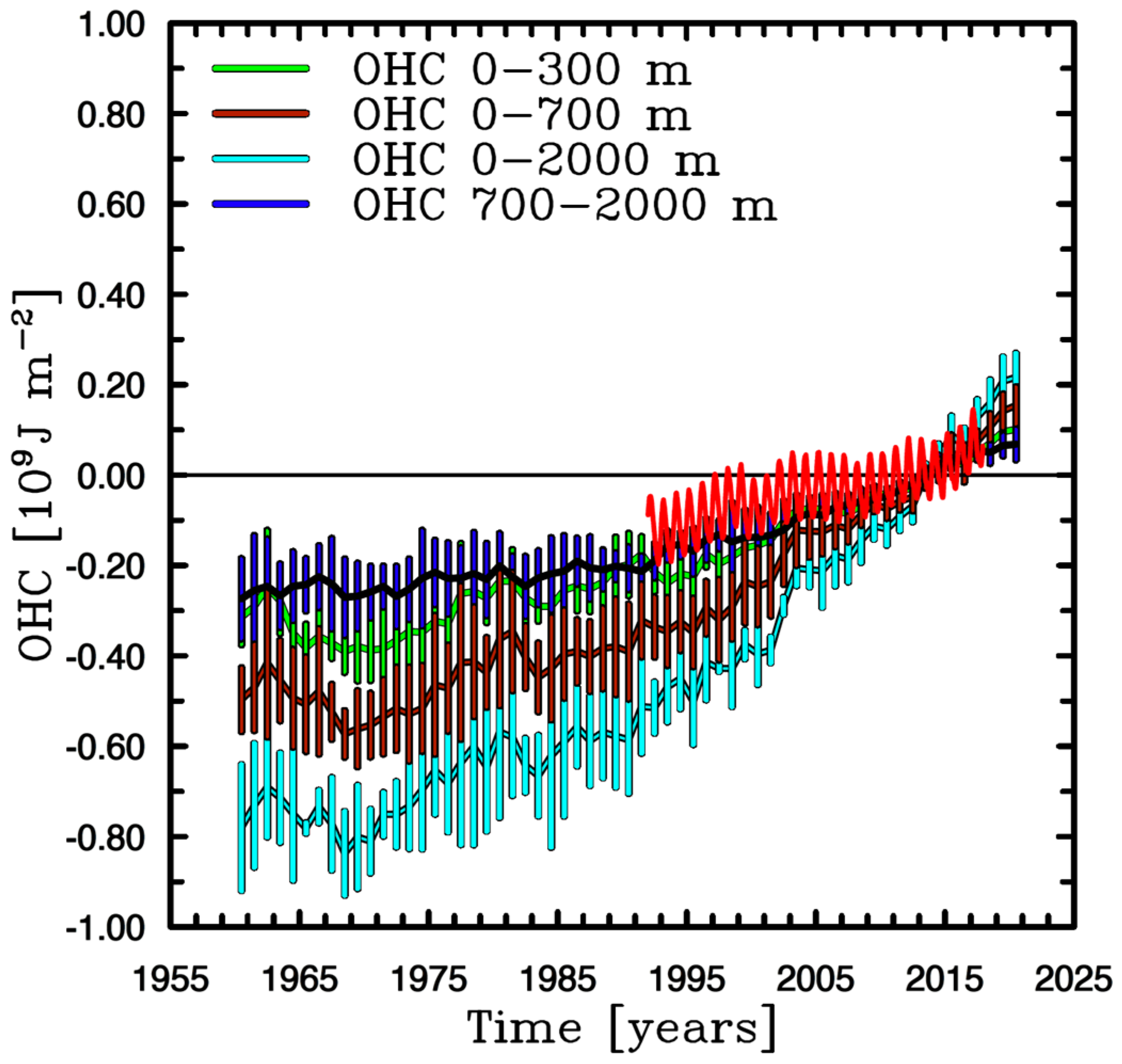

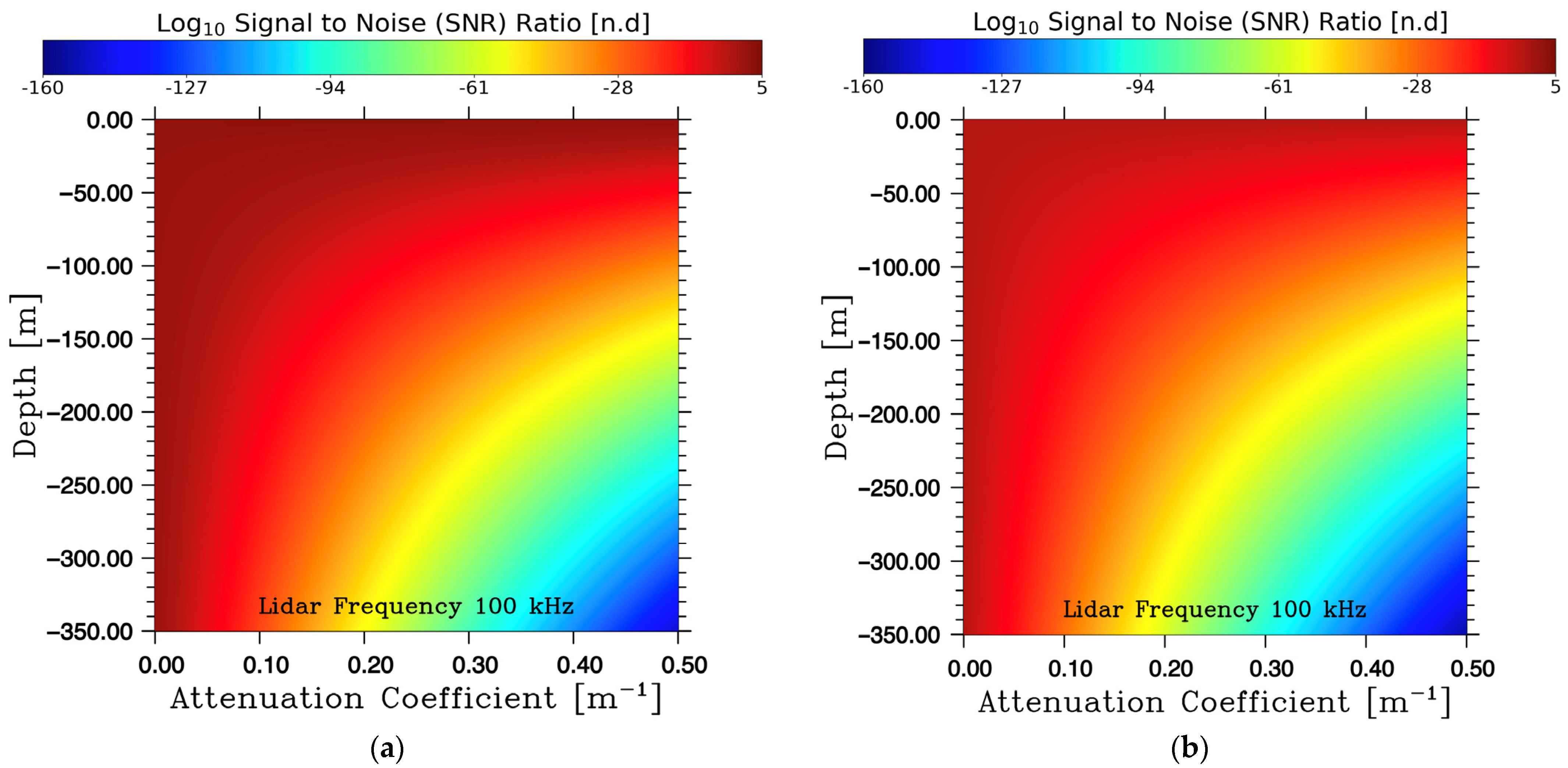
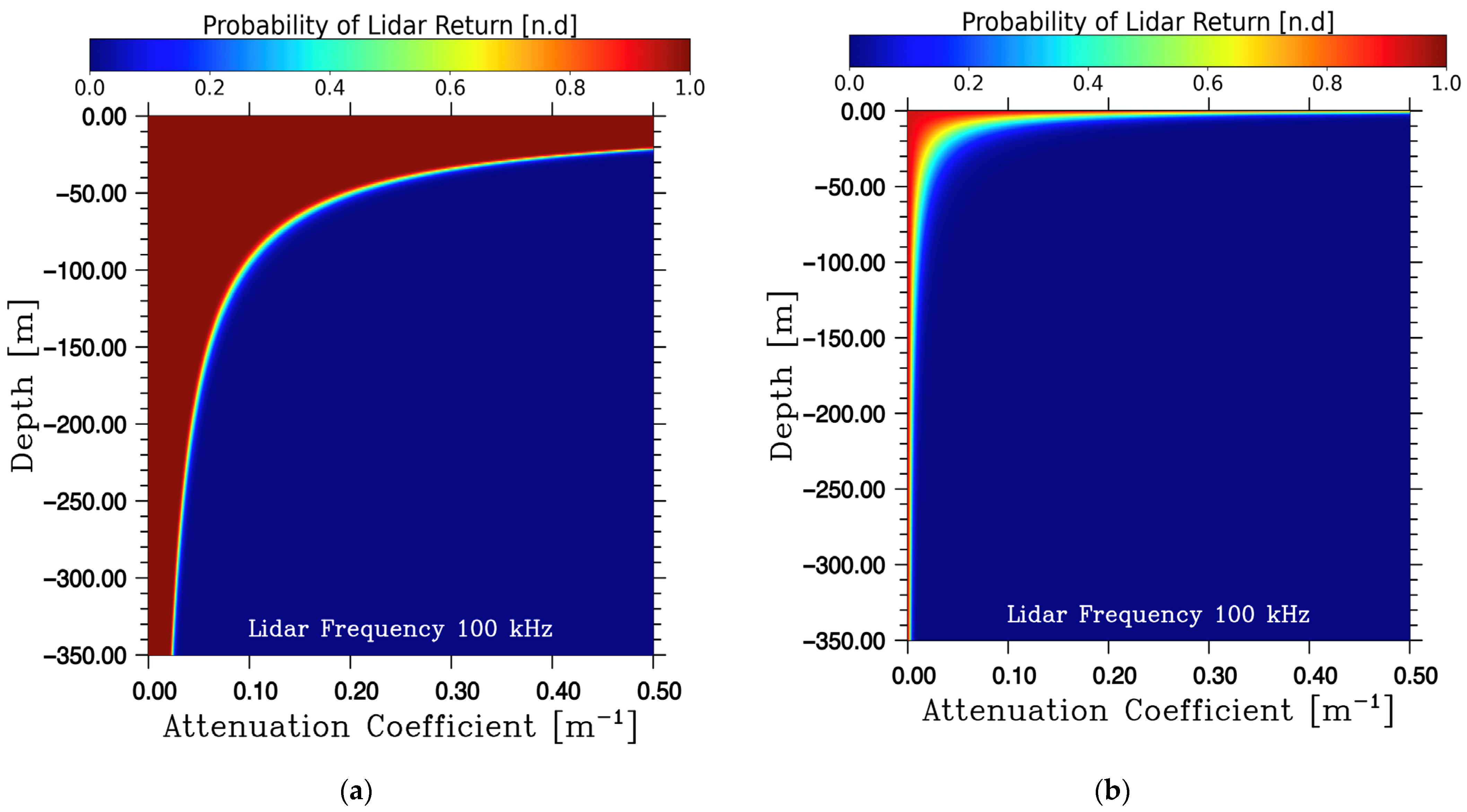

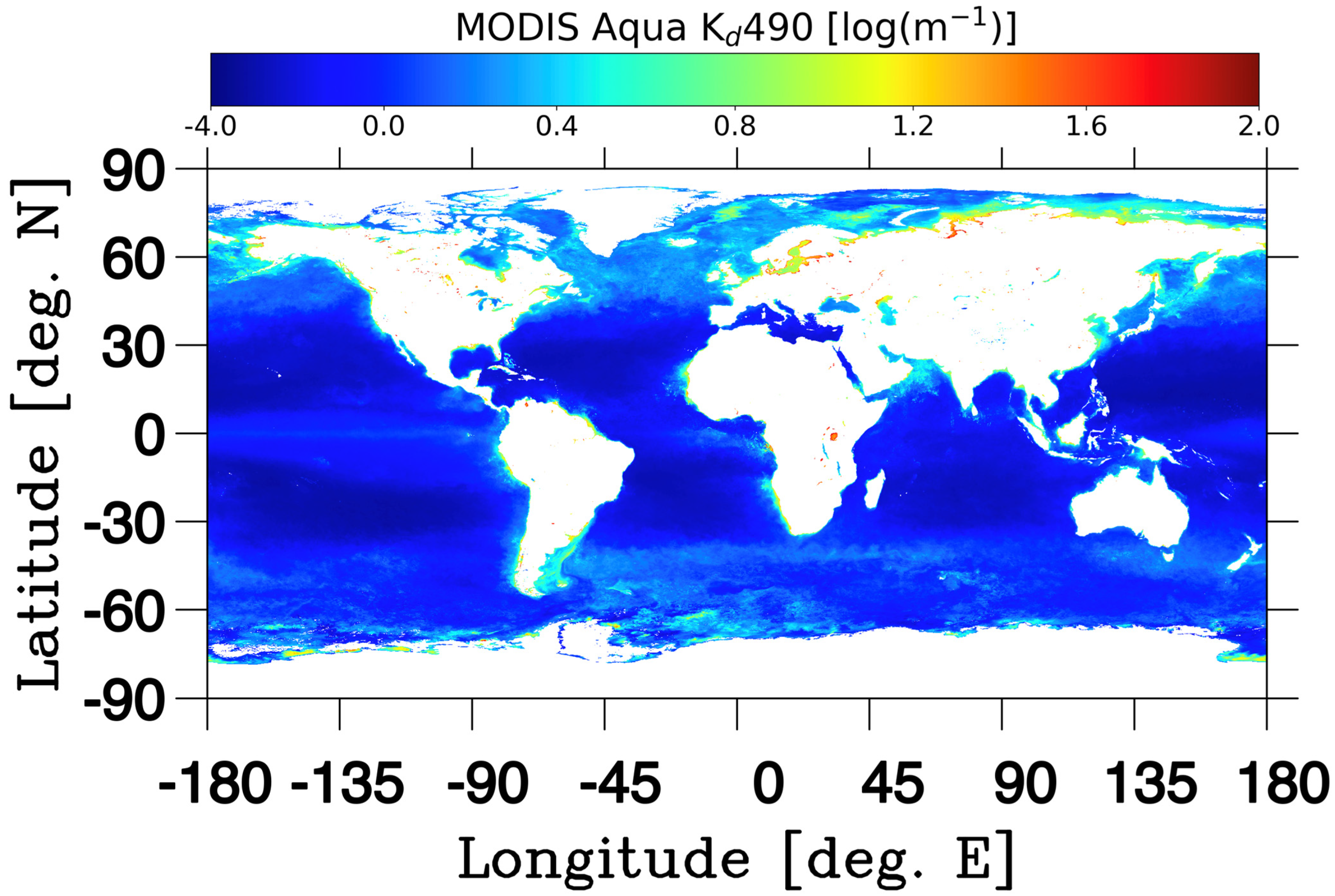
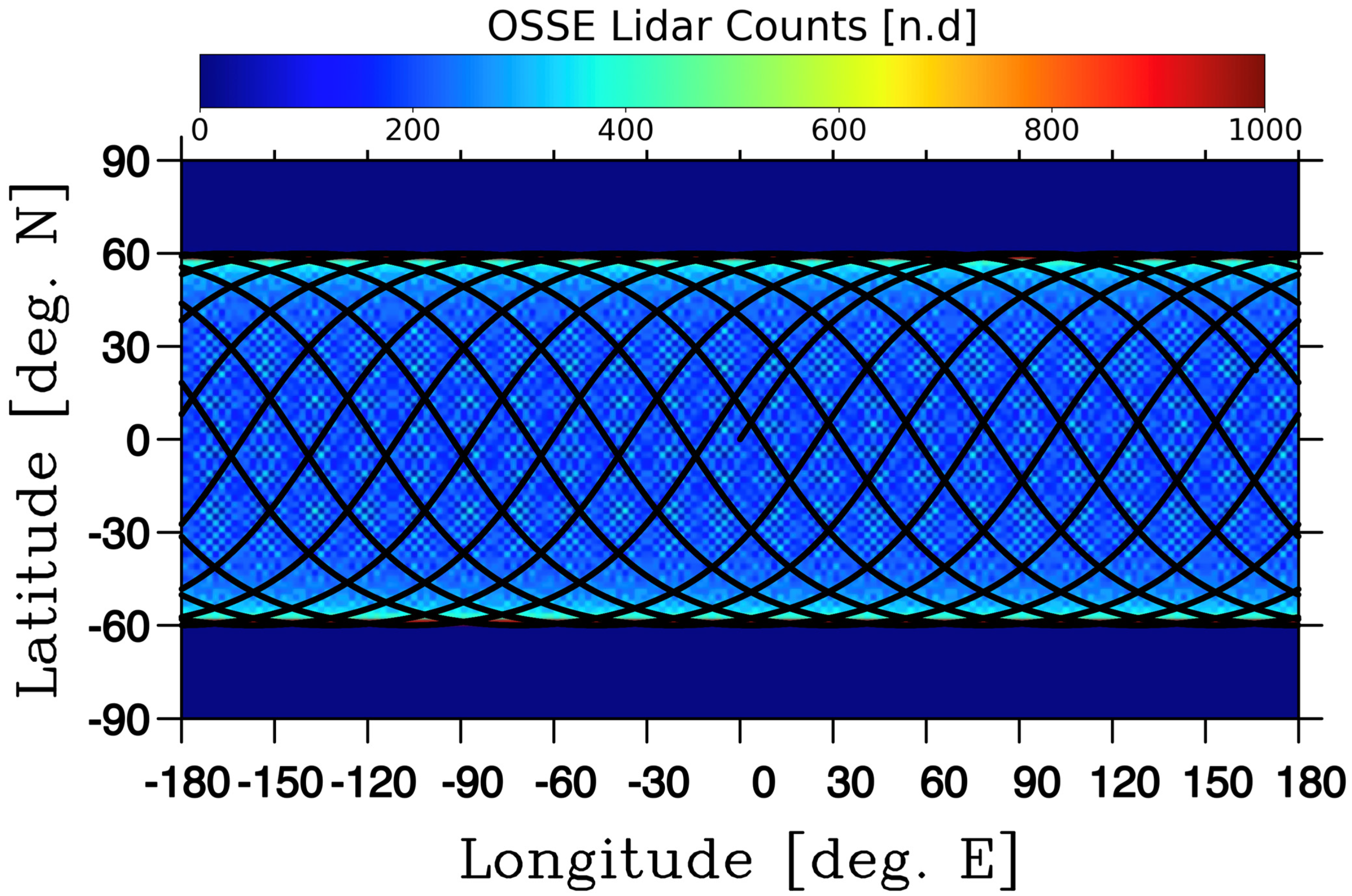
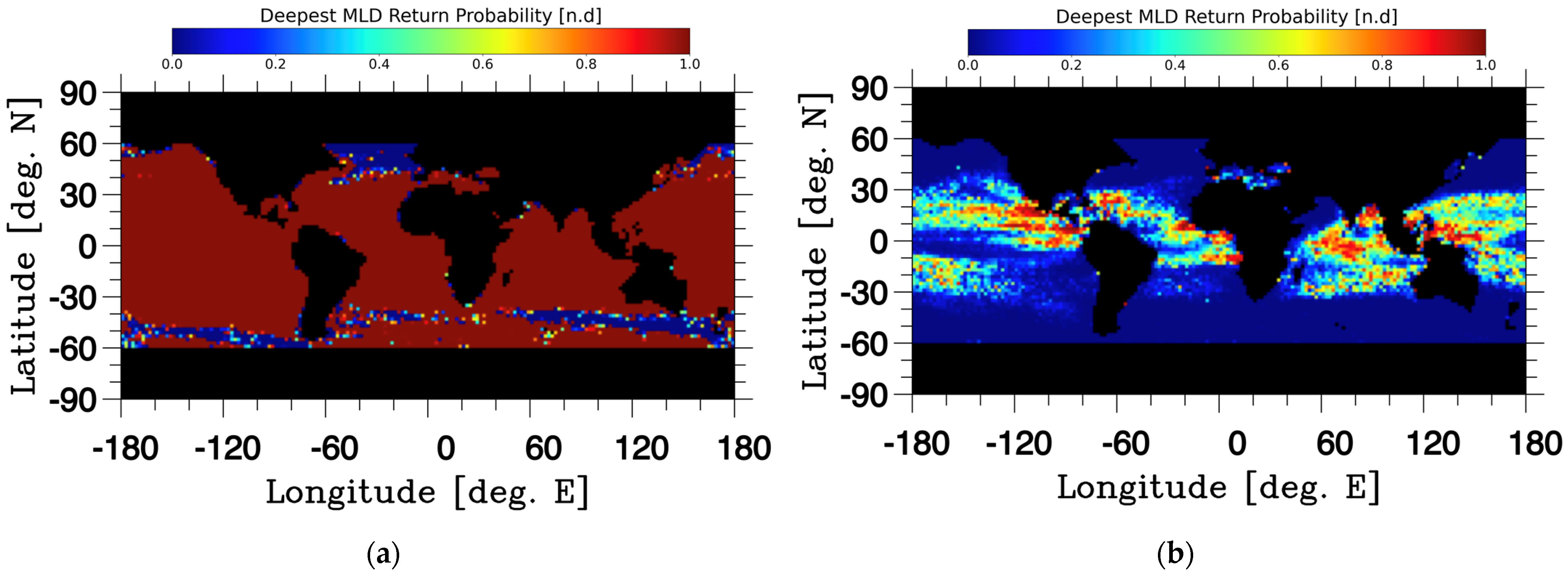
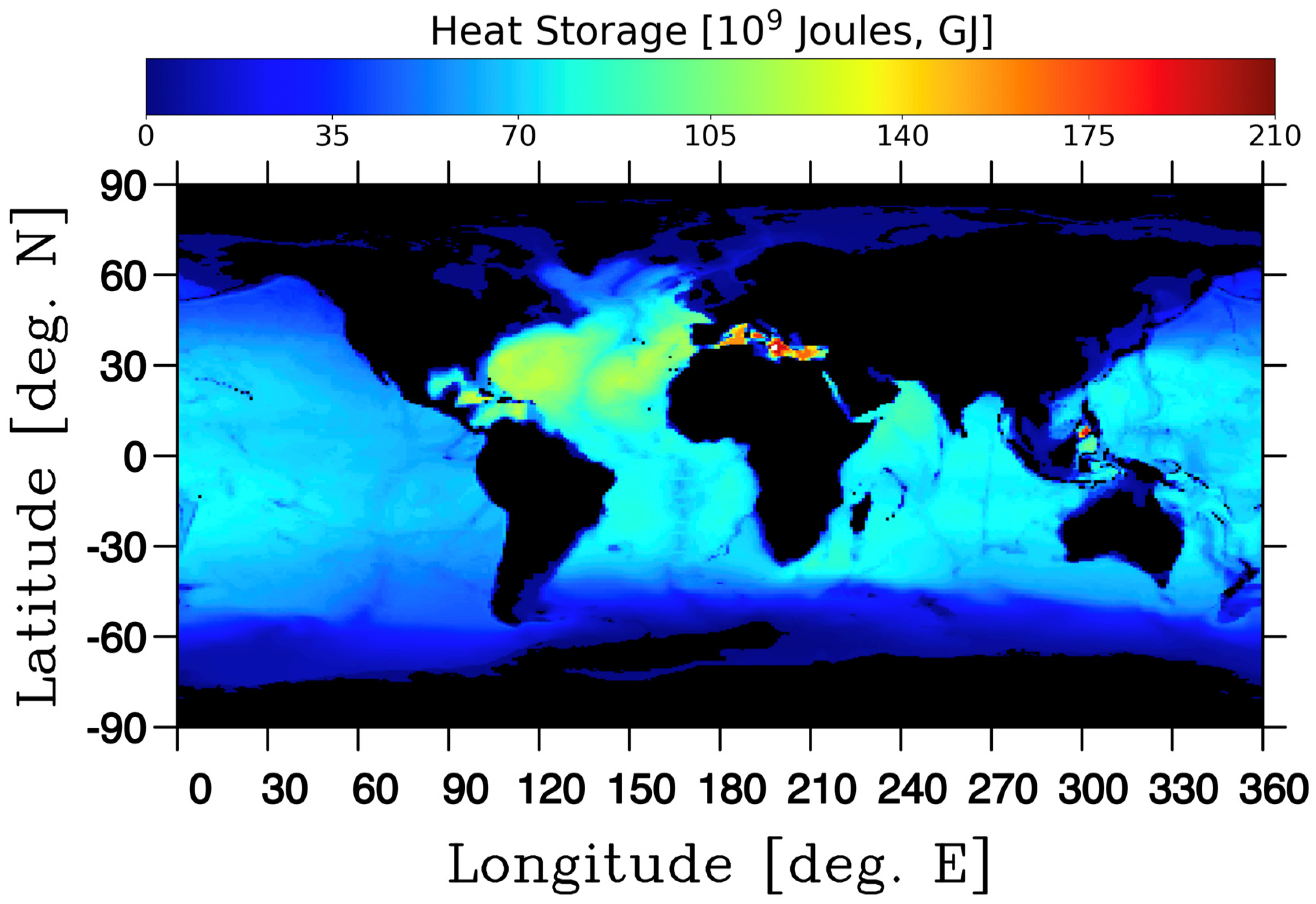
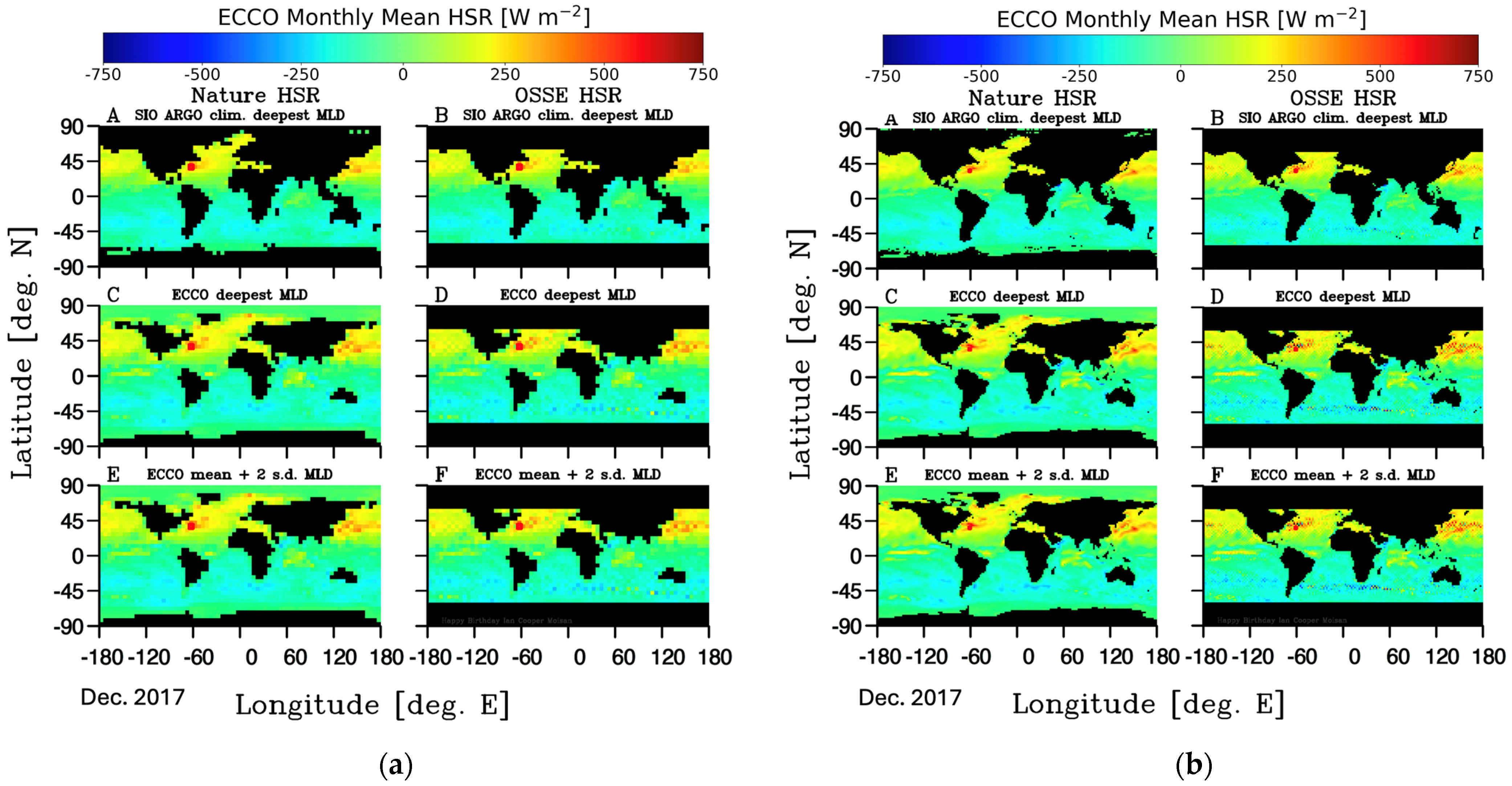

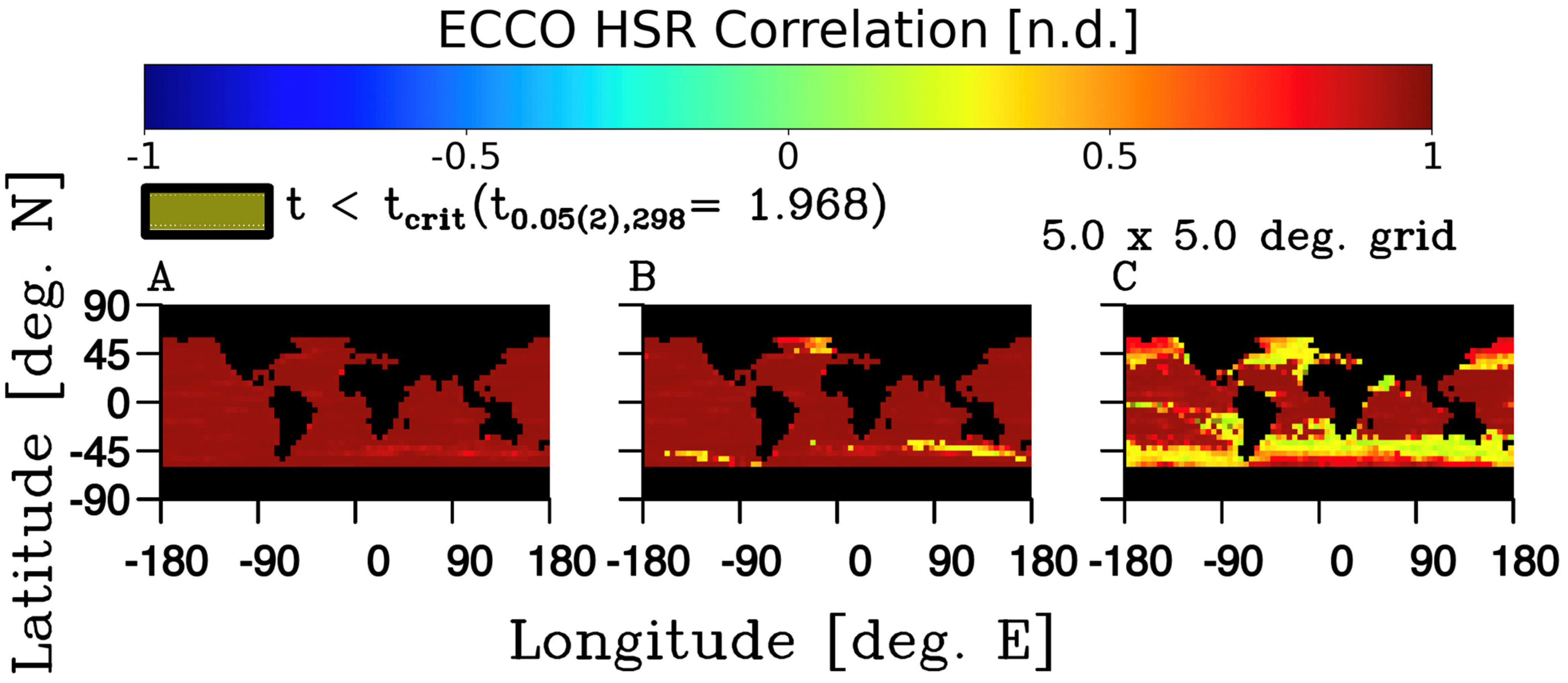
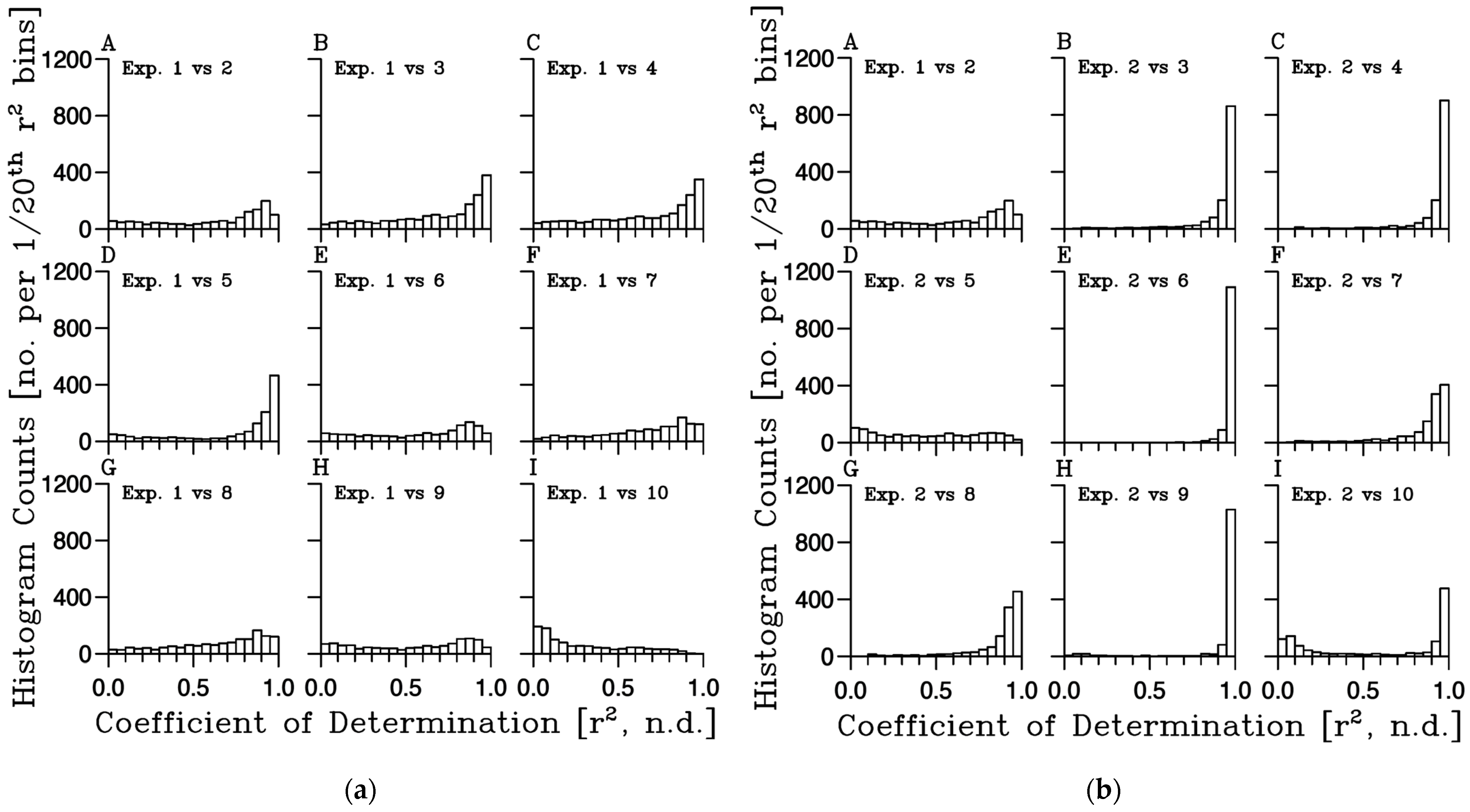
Disclaimer/Publisher’s Note: The statements, opinions and data contained in all publications are solely those of the individual author(s) and contributor(s) and not of MDPI and/or the editor(s). MDPI and/or the editor(s) disclaim responsibility for any injury to people or property resulting from any ideas, methods, instructions or products referred to in the content. |
© 2024 by the authors. Licensee MDPI, Basel, Switzerland. This article is an open access article distributed under the terms and conditions of the Creative Commons Attribution (CC BY) license (https://creativecommons.org/licenses/by/4.0/).