Abstract
Sea clutter usually greatly affects the target detection and identification performance of marine surveillance radars. In order to reduce the impact of sea clutter, a novel sea clutter suppression method based on chaos prediction is proposed in this paper. The method combines a generator trained by Generative Adversarial Networks (GAN) with a Long Short-Term Memory (LSTM) network to accomplish sea clutter prediction. By exploiting the generator’s ability to learn the distribution of unlabeled data, the accuracy of sea clutter prediction is improved compared with the classical LSTM-based model. Furthermore, effective suppression of sea clutter and improvements in the signal-to-clutter ratio of echo were achieved through clutter cancellation. Experimental results on real data demonstrated the effectiveness of the proposed method.
1. Introduction
Sea clutter is the radar echo reflected from the sea surface, which often seriously affects the radar’s performance in detection and identification of sea surface targets. Sea clutter suppression is important for radar observation of the sea. Therefore, a novel sea clutter suppression method based on chaos prediction is proposed.
Chaos is a phenomenon with potentially deterministic laws it follows, even though it may appear random. In 1995, S. Haykin et al. discovered that sea clutter is not completely random but typically chaotic [1,2]. The sea clutter sequence can be predicted according to the initial conditions by exploiting the inherent chaotic evolution law of sea clutter. Then, clutter cancellation is performed on the echo to improve the signal-to-clutter ratio (SCR).
The key to sea clutter prediction is to build non-linear models that describe the time-varying chaotic properties of sea clutter. Due to the use of non-linear activation functions, neural networks are well suited for non-linear fitting. N. Xie et al. utilized multiple radial basis function neural networks (RBFNNs) to model sea clutter [3]. For further improvement, an adaptive artificial neural networks (ANNs) ensemble approach and an improved general regression neural networks algorithm were introduced [4,5]. In contrast to these static networks, recurrent neural networks (RNNs) are more suitable for modeling non-linear dynamic systems due to the capability of hidden nodes to record historical information [6,7]. With the improvement of RNNs, long short-term memory (LSTM) networks demonstrate better performance in the learning of sea clutter’s long-term variation law, and achieve smaller prediction errors than RBFNNs and ANNs [8,9,10].
Inspired by generative adversarial networks (GANs) for learning the distribution of unlabeled data [11,12,13], this paper combined the generator and LSTM networks to predict sea clutter. The generator was firstly trained in GANs, and then used with LSTM networks to bring more clutter evolution information, which helped improve the prediction accuracy. Furthermore, sea clutter was suppressed through the sea clutter cancellation process.
The organization of this paper is as follows. In Section 2, the LSTM-based sea clutter prediction model is modified by replacing the fully connected layer with a generator for higher prediction accuracy. In Section 3, a new sea clutter suppression method using chaotic prediction is introduced. In Section 4, the experimental results of real data are shown to demonstrate the effectiveness of the proposed method. In Section 5, this paper is concluded.
2. Sea Clutter Prediction Model
Sea clutter is a chaotic sequence generated by a corresponding non-linear dynamic system [1]. represents a sea clutter sequence, where . According to the Takens’ embedding theorem [14], an equation for sea clutter prediction is introduced [1]:
where , m denotes the embedding dimension and τ denotes the time delay [15]. represents a nonlinear mapping function.
Since the intrinsic properties of such dynamic systems are deterministic rather than random, the variation of sea clutter in time or space is regular. The key to sea clutter prediction is to learn the evolution laws in the sea clutter sequences.
2.1. Classical LSTM-Based Prediction Model
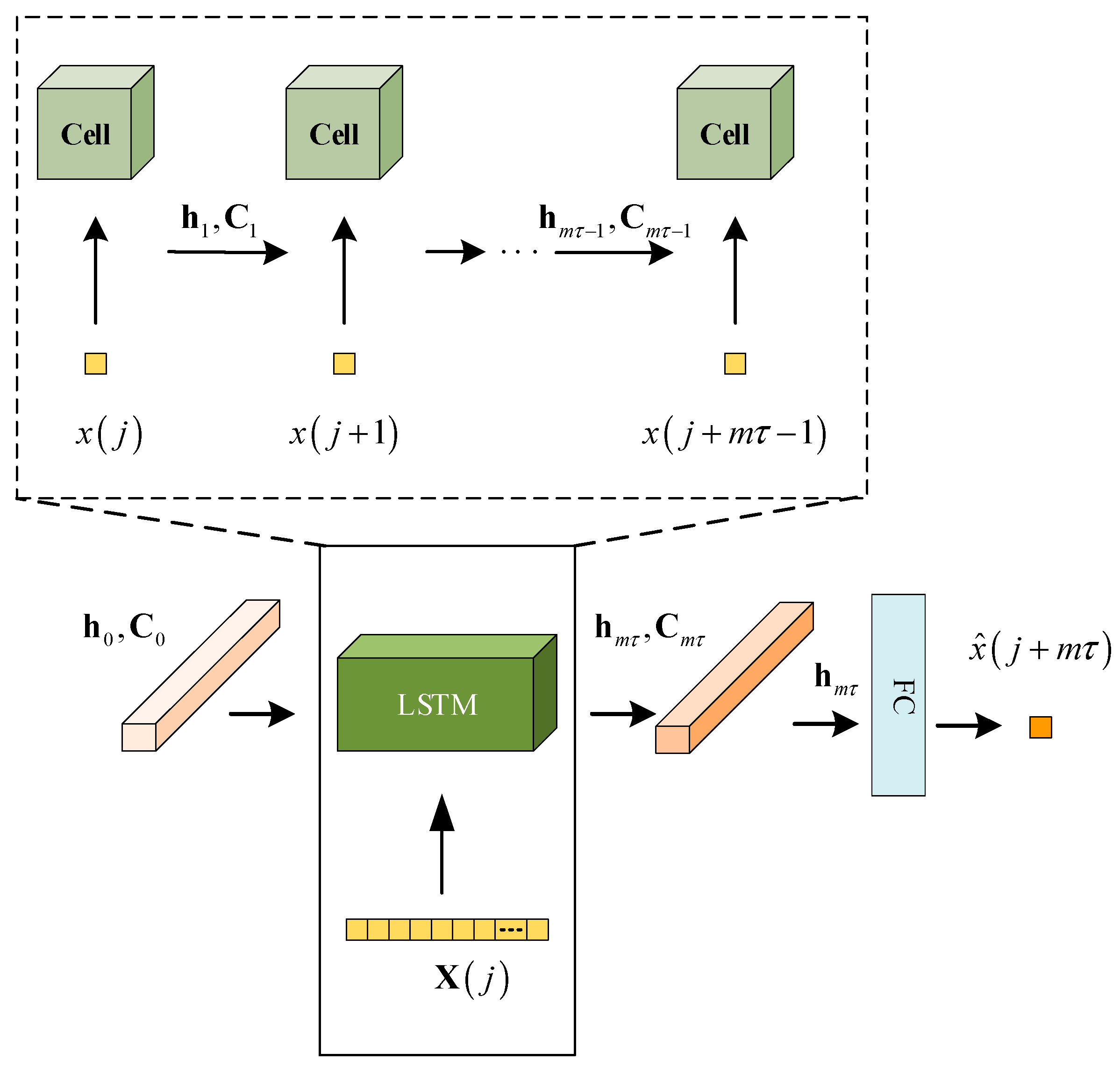
Based on Equation (1), an LSTM-based sea clutter prediction model is trained. Figure 1 demonstrates the LSTM-based prediction model, which is mainly composed of an LSTM network and a fully connected (FC) layer. Under the excitation of the input sea clutter sequence , a randomly initialized hidden vector and a memory cell state vector , the LSTM network outputs a latent vector , which contains the evolution information in . Then, the FC layer decodes to generate the predicted result , which is expected to be close to the ground truth . Using the acquired sea clutter data, the LSTM-based model is trained to fit the one-step prediction.
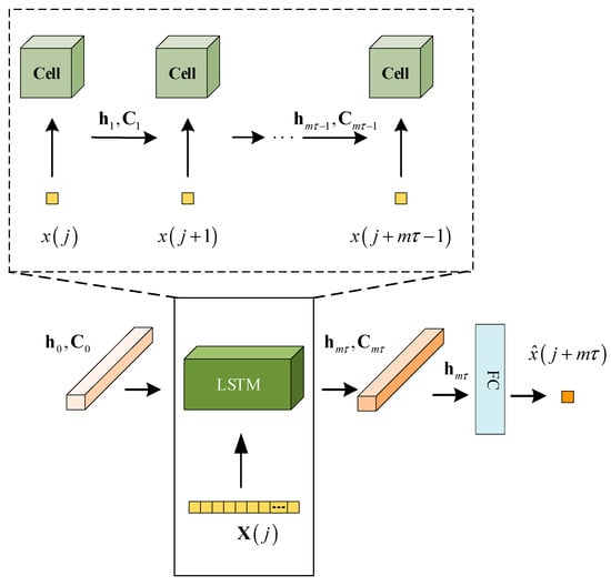
Figure 1.
An LSTM-based neural network model used for one-step sea clutter prediction. The LSTM network encodes the input sequence into a vector that contains the evolutional law in . Then, the FC decodes the vector into , which is the predicted value of next time. The LSTM network contains the cell, which works in the recurrent mechanism. At the t-th moment, the cell has three inputs. One is . The other two are the hidden vector and the memory cell state vector , which are the outputs of the cell at the time . The cell memorizes the state of the previous input, continuously updates the latest input information, and passes it on, so that the vector has the evolutionary information of the whole input sequence .
2.2. Improved Prediction Model Combining the Generator and LSTM Networks
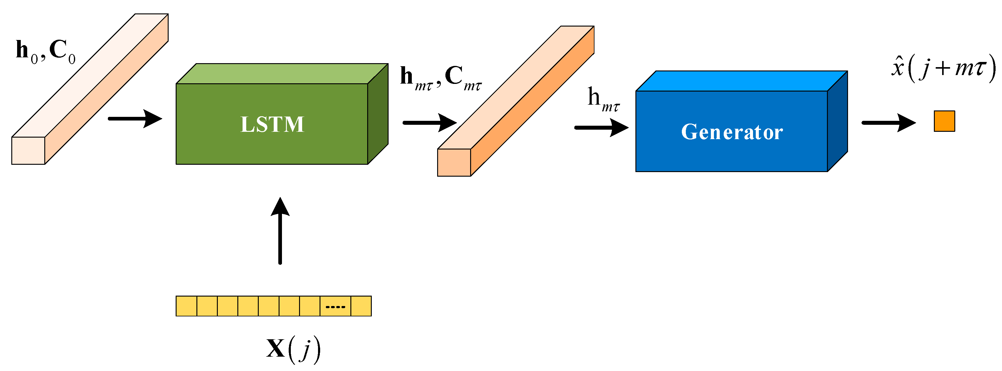
As for the aforementioned LSTM-based model, the FC layer can only accomplish linear decoding, which restricts its nonlinear mapping ability. For further improving the accuracy of sea clutter prediction, a modified prediction model combining the generator and LSTM (GLSTM) networks is proposed in Figure 2.
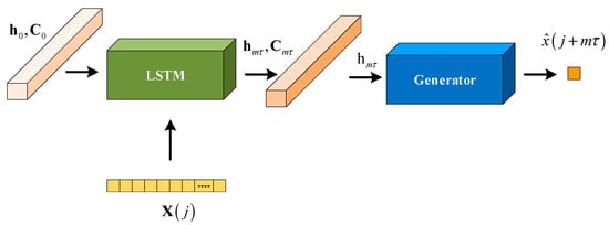
Figure 2.
A GLSTM-based model for one-step prediction of sea clutter sequences. The input of the model is a sea clutter sequence that is encoded into a vector . Then, the generator obtained by adversarial training decodes into the predicted element.
In the modified model, the FC layer is replaced by a generator, which plays a role in minimizing the Jensen–Shannon (JS) divergence between the generated distribution and the real sea clutter distribution [16]. JS divergence is a measure of similarity or dissimilarity between two probability distributions. The LSTM networks obtain the latent vector from the input sequences and pass the evolution information to the generator. Then, the generator produces the predicted results. Compared with the FC layer, the predicted results provided by the generator are more consistent with the statistical characteristics of sea clutter, which are obtained by solving the following optimization problem:
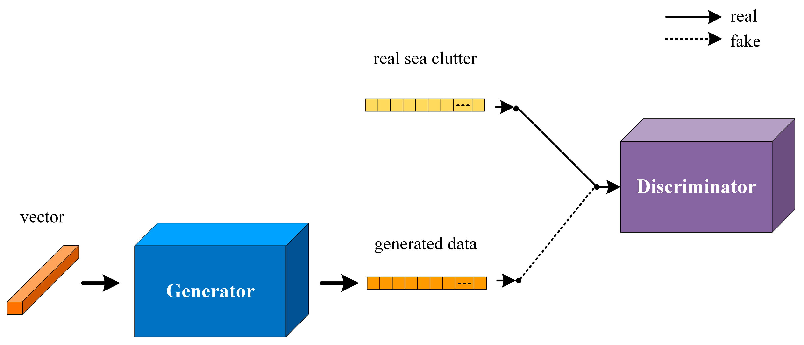
where is the conditional probability that measures the similarity between the predicted result and ground truth, refers to the LSTM, refers to the generator, and is the predicted result that maximizes . When is the maximum, the JS divergence becomes minimum. The generator is obtained by adversarial training with a discriminator, as shown in Figure 3. Vectors with the same dimension as the latent vector are input to the generator. Then, the real sea clutter vector and the generated vector are fed into a discriminator. The discriminator is optimized so as to distinguish two inputs as much as possible. The generator is simultaneously trained to make the discriminator confused by the two inputs as much as possible. During the adversarial training, the discriminator and generator become more powerful and finally reach a point at which both cannot be improved. This means that the training of the generator has been completed.

Figure 3.
The training process involves a generator and a discriminator to learn the distribution of sea clutter. The generator accepts a fixed dimensional vector and generates data, while the discriminator evaluates whether the input is real sea clutter or generated data and provides the corresponding judgment results.
After the generator is well trained, it is fixed and put into the model as shown in Figure 2. By taking advantage of the ability to produce data similar to real sea clutter, the generator decodes the latent vector and provides the sea clutter prediction with higher accuracy.
3. Sea Clutter Suppression Based on Chaotic Prediction
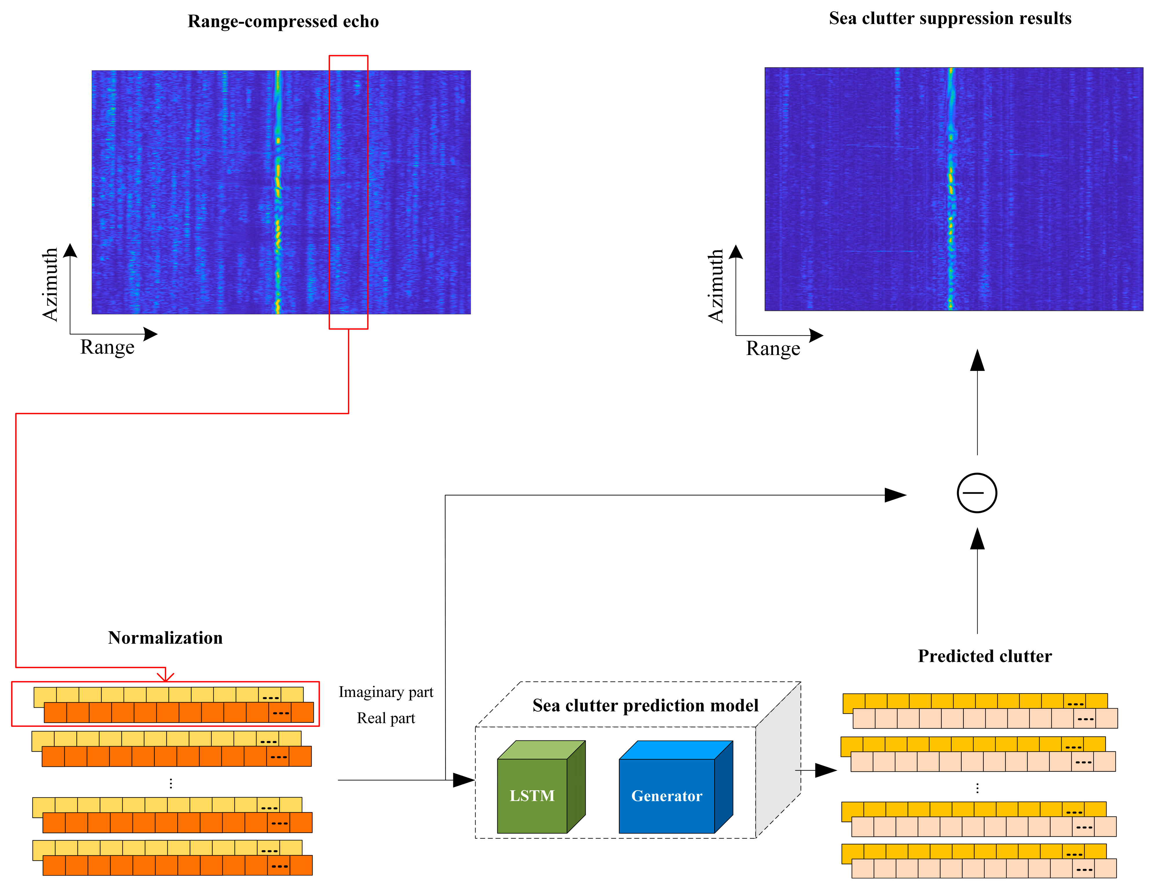
Figure 4 shows the proposed GLSTM-based prediction model. As shown in the red rectangle in Figure 4, the range cells are processed one by one. Firstly, the real and imaginary components are normalized. Subsequently, the normalized parts are put into the sea clutter prediction model, which generates the predicted clutter result. At last, the predicted clutter result is subtracted from the original data to get the sea clutter-suppressed result.

Figure 4.
Sea clutter suppression using chaotic prediction. The range cells are processed one by one. Firstly, the real and imaginary components are normalized. Subsequently, the normalized parts are put into the sea clutter prediction model, which generates the predicted clutter. At last, the predicted clutter is subtracted from the original data to get the sea clutter-suppressed result.
3.1. Echo Normalization and Denormalization
The original data are normalized per range cell [17]. The normalization formula is:
where denotes the real or imaginary part of the sea clutter sequence in each range cell, is the normalized result of , represents the minimum values of and represents the maximum values of .
The denormalization formula is:
where is the normalized real or imaginary part of the sea clutter sequence, is the denormalized result of . and are the data recorded during the normalization process.
3.2. GLSTM-Based Model Training
Before performing sea clutter elimination, the prediction model must be trained to ensure that it effectively learns the chaotic evolution laws of sea clutter.
According to Equation (1), normalized sequences, with a length of in a chosen range cell where no targets are present, are employed for model training.
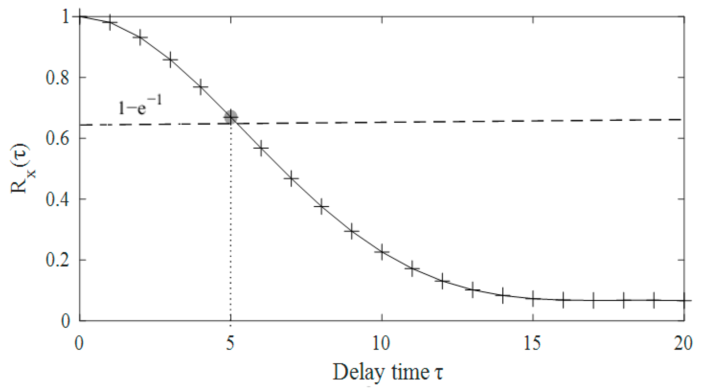
The optimal delay time τ is determined by calculating the autocorrelation function and is expressed as:
where * denotes a complex conjugate process. The optimal delay time is selected when decreases to of its maximum value [15].
The Cao algorithm is employed for the estimation of the embedding dimension m [18]. The time delay vector is reconstructed as:
where . represents the j-th time-delay vector when the embedding dimension is m.
The function is employed to ascertain the minimum embedding dimension m and is expressed as:
where , is given by:
and are the k1-th and k2-th time delay vector, respectively. and are the s-th element of the k1-th and k2-th time delay vector, respectively. is the j-th time delay vector with embedding dimension m + 1. is an integer from 1 to , is the nearest neighbor of in the sense of distance defined in Equation (8). The average value of across j is expressed as:
Moreover, is employed to examine the change in , which is expressed as:
will not obviously change if m exceeds a certain value . At this point, is identified as the minimum embedding dimension.
As illustrated in Figure 5, sequences of length are obtained and the labels associated with these sequences are chosen to construct the training dataset. Then, training can be performed.
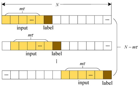
Figure 5.
Training dataset. With an original sequence of length N, the training dataset is created by obtaining short sequences of length and their corresponding labels.
As mentioned in Section 2.2, the training of the GLSTM-based prediction model includes two steps. Firstly, the deep convolutional generative adversarial networks are built to train the generator to learn the characteristics of sea clutter. The batch size is 64, the learning rate is 0.0002, the number of training iterations is 100, and the loss function is the cross entropy function. After the completion of generator training, the training of the LSTM is started. The specifications for this phase include an LSTM network with 2 layers, 100 hidden nodes, a batch size of 64, a learning rate of 0.0002, and 25 training iterations. The loss function selected is the mean squared error. Throughout both training steps, the Adam algorithm is employed for optimizing parameters. The resultant GLSTM-based prediction model is suitable for processing radar and marine environmental parameters corresponding to the echo data.
3.3. Sea Clutter Estimation and Cancellation
The trained GLSTM-based prediction model is sequentially applied to the range-compressed echo data. The model estimates the sea clutter within the echo, allowing for the subsequent cancellation of the original data with the predicted sea clutter result. This process achieves the suppressed sea clutter result.
4. Experimental Results and Analysis
The proposed GLSTM-based method was validated using range-compressed data supplied by the Naval Aeronautical University [19,20].
4.1. Experimental Data
A stationary radar was used to acquire the echo data, and the polarization was HH. The sea state at that time was level 3–4.
Two blocks of range-compressed data were selected for validating the proposed method. For data Block I, there are 4346 range cells and 6940 pulses, with no targets present. Data block II consists of 4346 range cells and 4390 pulses, with target signals predominantly located in the 940–953, 1482–1492, and 2140–2810 range cells.
In order to conduct a more comprehensive analysis, the training dataset contained blocks with strong clutter energy targets and no targets. Before the GLSTM-based model was trained, two key parameters needed to be determined as mentioned in Section 3.2. τ can be determined according to the autocorrelation function, and m can be determined according to the Cao algorithm.
Figure 6 shows a curve example corresponding to the normalized autocorrelation function. The optimal delay time τ = 5 achieves equality.
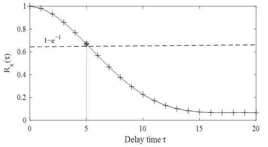
Figure 6.
The curve corresponding to the normalized autocorrelation function. The delay time τ must be an integer. The horizontal line represents , and the vertical line represents m = 5. is nearest to when τ is set to 5, which is shown in the gray circle.
Figure 7 denotes obtained through the application of the Cao algorithm. Stability can be observed in after m = 9, which determines a minimum embedding dimension of 10. For data block I, where each range cell has a pulse number of 6940, the training dataset can be built with 6890 sequences, each of 50 lengths. Similarly, for data block II, τ = 3 and m = 14 are optimal, and the training dataset contains 4348 short sequences.
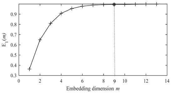
Figure 7.
The variation of increases as the embedding dimension m increases. The growth rate of the curve becomes very slow when m is greater than 9. The gray circle indicates the position of the curve at m = 9.
4.2. Subjective Evaluation of Sea Clutter
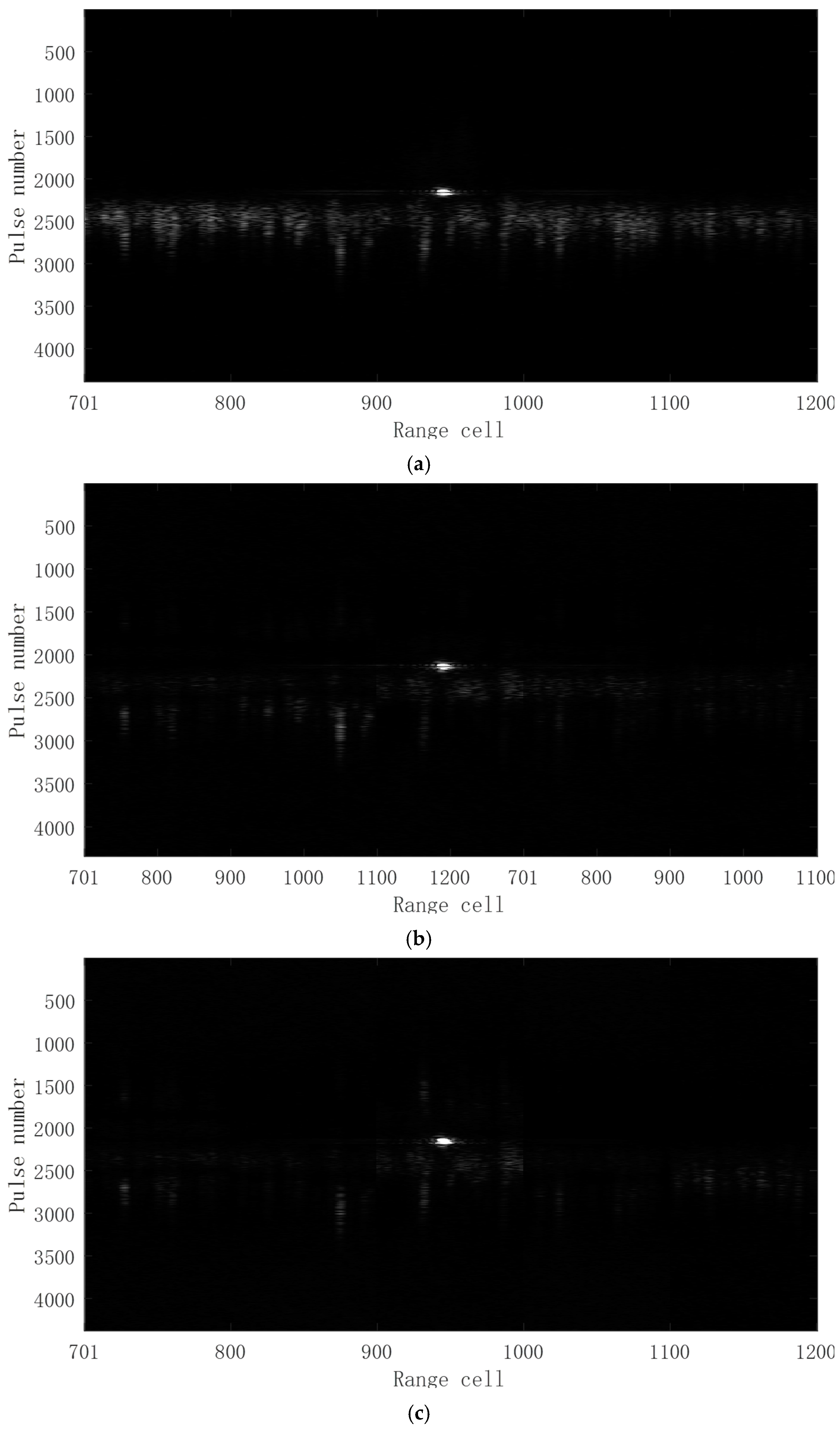
The amplitude images for range cells 701–1200 are shown in Figure 8. The radar echo data contains ship target signals within the 940–953 range cells, with high clutter amplitude in the surrounding sea clutter. Figure 9 shows the corresponding images of Figure 8.
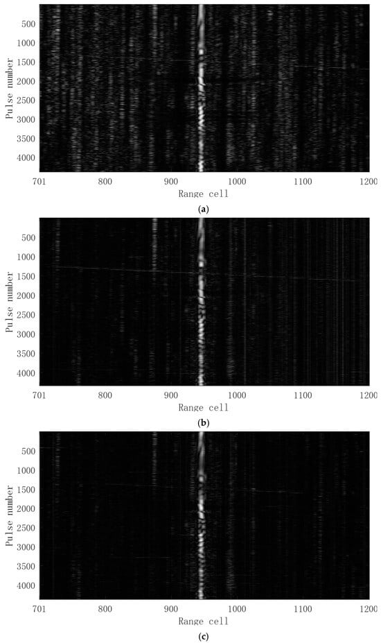
Figure 8.
Range compression amplitude image of radar echoes. (a) Range compression amplitude image of the original radar data. (b) Range compression amplitude image of the LSTM-based method-suppressed result. (c) Range compression amplitude image of the GLSTM-based method-suppressed result.

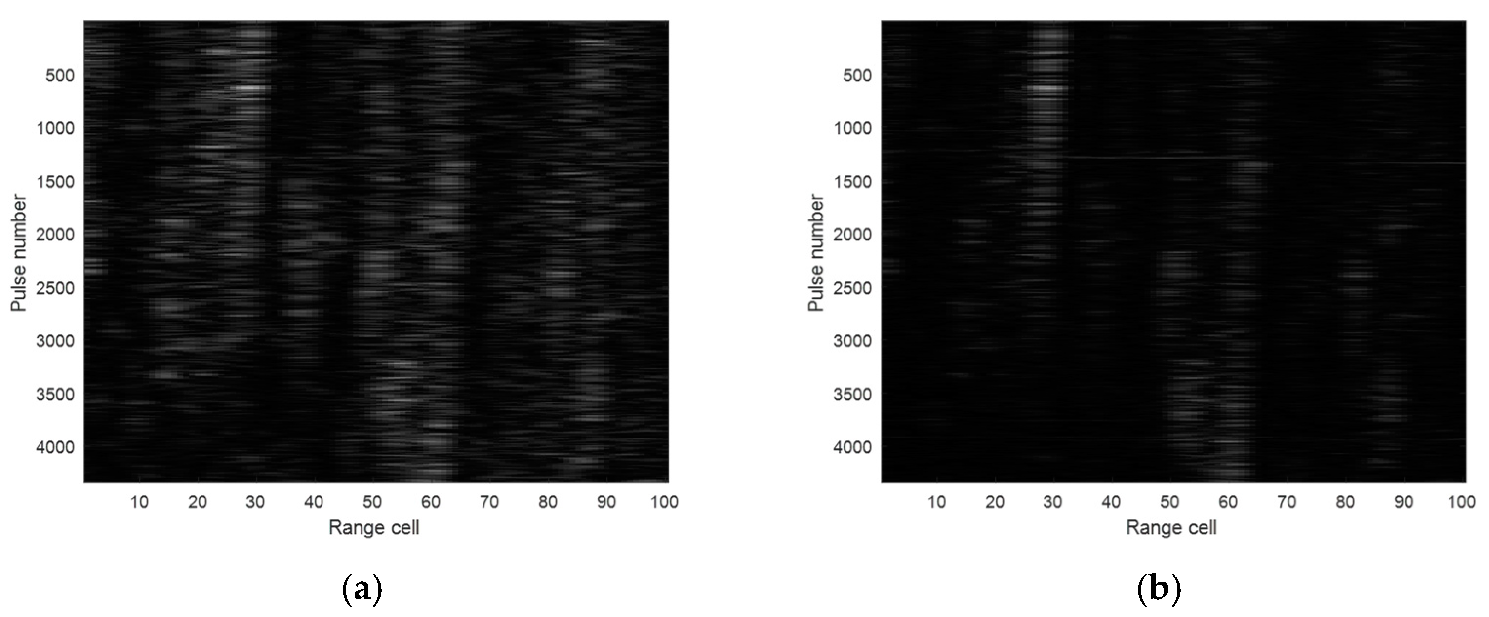
Figure 9.
Image of radar echoes. (a) Image of the original data. (b) Image of the LSTM-based method suppressed result. (c) Image of the GLSTM-based method suppressed result.
As shown in Figure 8 and Figure 9, both LSTM-based and the proposed GLSTM-based method were capable of effectively suppressing sea clutter, while the GLSTM-based method exhibiting better suppression performance. After sea clutter suppression using the GLSTM-based method, the amplitude of the target signal remained relatively high, while the amplitudes of the surrounding sea clutter signals were significantly reduced. This led to a cleaner background in the imaging results. Through calculation, using the LSTM-based method, the SCR could be increased by 3.8 dB. In contrast, the use of the GLSTM-based method could result in a larger increase, with a 6.1 dB improvement in SCR.
4.3. Prediction Accuracy of Sea Clutter
R-squared, also known as the coefficient of determination, is applied to evaluate the prediction accuracy [21], which is:
where denotes the ground truth, denotes the predicted result, and denotes the mean of . The formula essentially compares how well the model performs compared to a simple model that uses the mean of the dependent variable to make predictions. The higher the R-square value (close to 1), the better the prediction effect of the model.
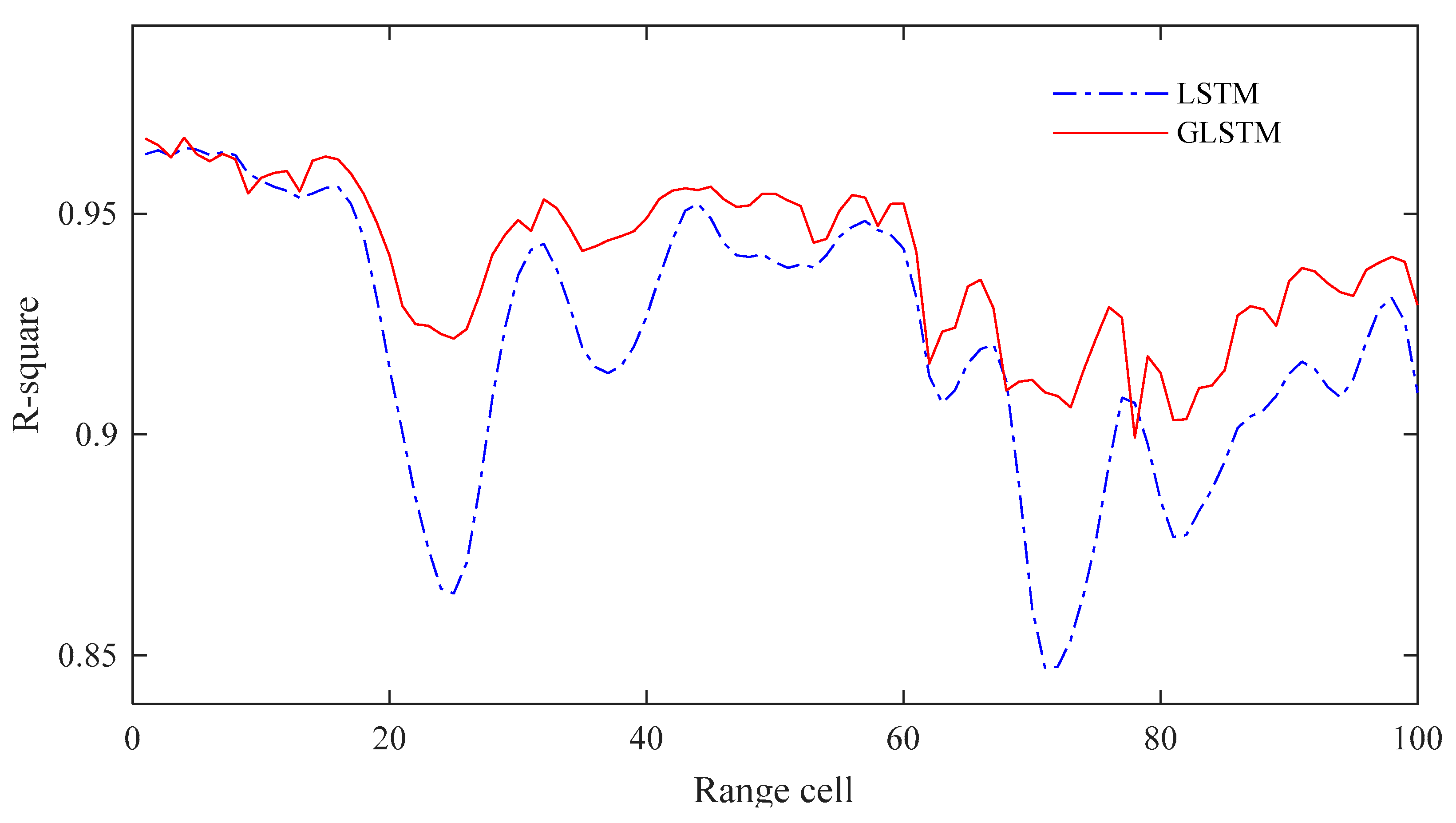
Figure 10 demonstrates R-square curves obtained by processing data block I in the 2–100 range cells based on the LSTM-based and GLSTM-based models. The GLSTM-based model had a prediction accuracy improvement of 0.07%–6.2% better than that of the LSTM-based model in 92% of the range cells, and 0.03%–0.78% worse in the rest of the range cells. The average R-square coefficients achieved by the GLSTM-based and LSTM-based models were 93.84% and 92.89% respectively, which demonstrate that the proposed sea clutter prediction model outperforms the classical LSTM-based model in prediction accuracy.
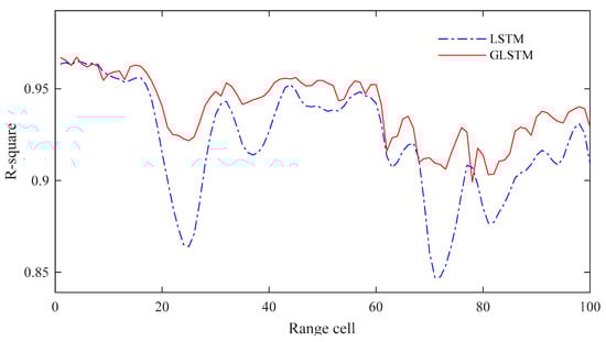
Figure 10.
R-square curves obtained by processing data block I in the 2–100 range cells based on the LSTM-based and GLSTM-based models.
4.4. SCR Improvement
Figure 11 shows the sea clutter suppressed results for data block I in the 58th range cell where no targets exist. Figure 11a and Figure 11b compare the original data with the results of the LSTM-based and GLSTM-based methods, respectively. The sea clutter energy is suppressed by 10.3 dB and 11.8 dB on average in Figure 11a and Figure 11b, respectively.
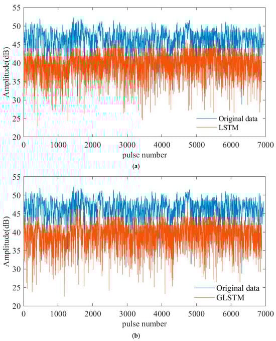
Figure 11.
Sea clutter suppression results of data block I. (a) The comparison of the original data and the clutter suppression result of the LSTM-based method. (b) The comparison of the original data and the clutter suppression result of the GLSTM-based method.
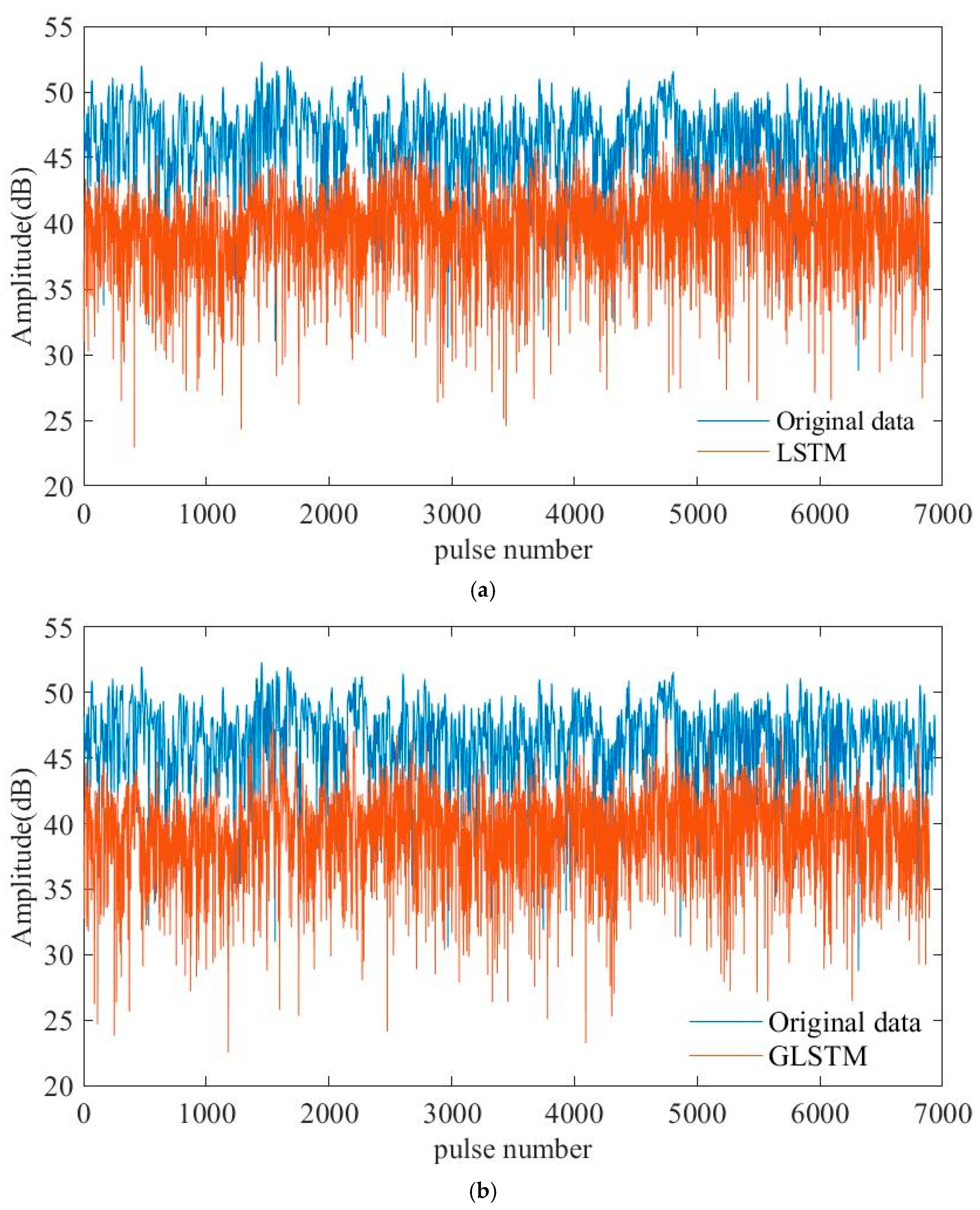
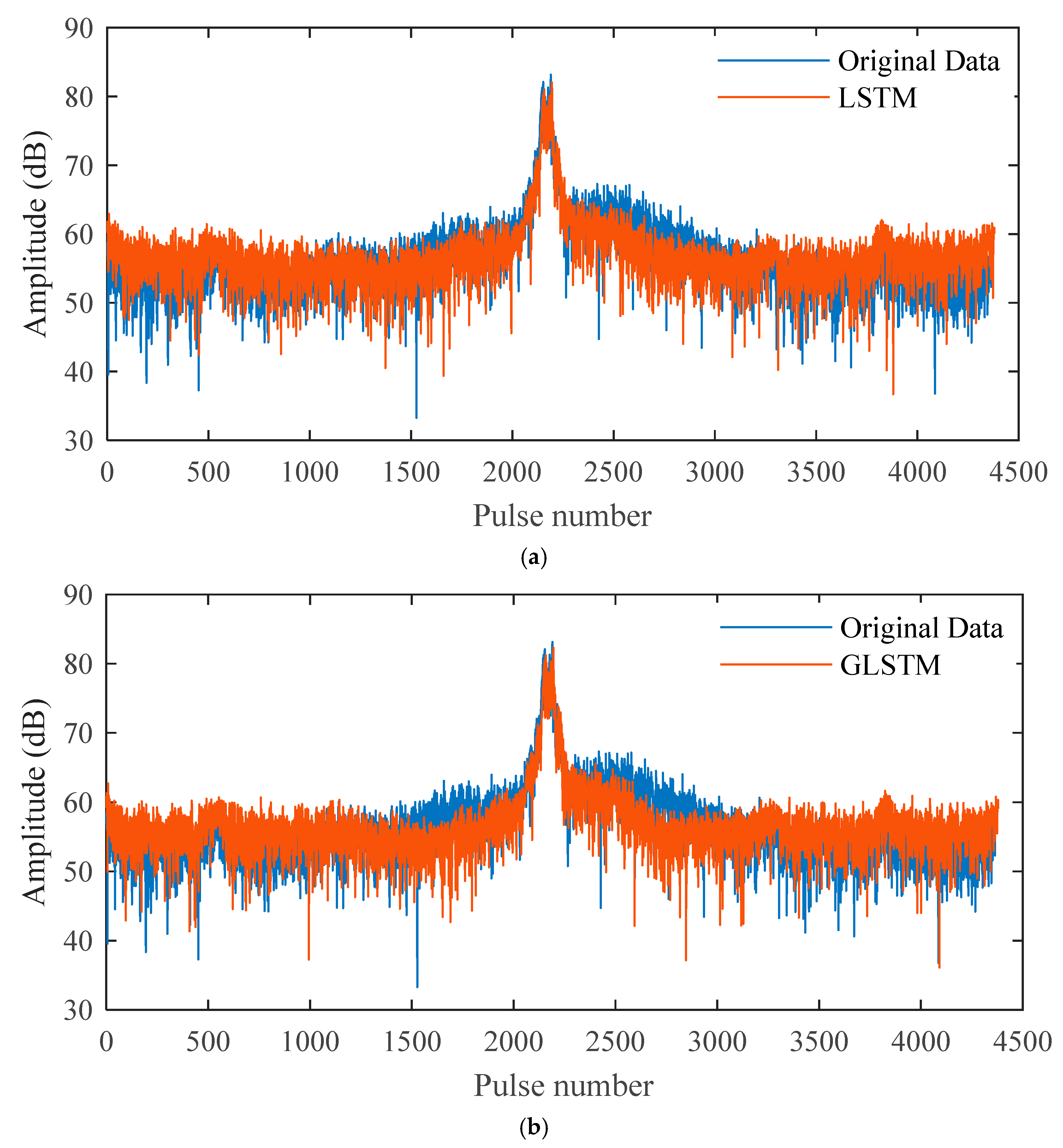
Figure 12 shows the sea clutter suppressed results for data block II in the 945th range cell with a target existing. Figure 12a and Figure 12b offer a comparison between the LSTM-based and GLSTM-based method results, respectively. The LSTM-based and GLSTM-based methods improved the SCR by 3.8 dB and 6.1 dB, respectively.
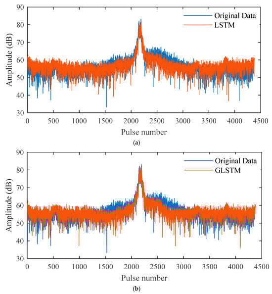
Figure 12.
Sea clutter suppressed results of data block II. (a) The comparison of the original data and the clutter suppression result of the LSTM-based method. (b) The comparison of the original data and the clutter suppression result of the GLSTM-based method.
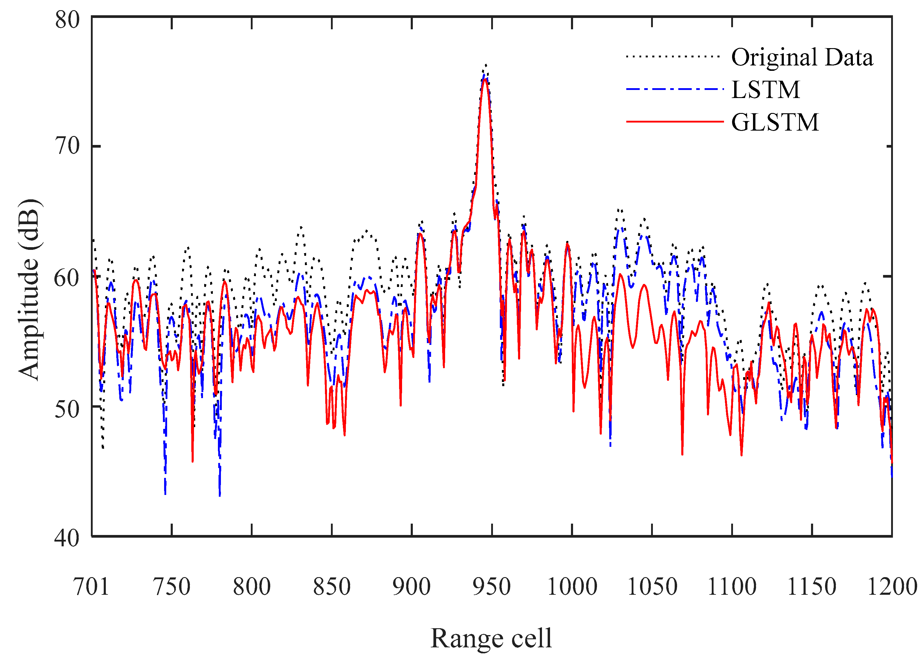
For data block I where no targets exist, Figure 13 contrasts the result curves of the 4000th pulse, which indicates that the GLSTM-based method is superior to the LSTM-based method in sea clutter suppression.
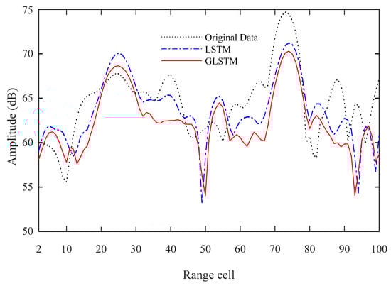
Figure 13.
The sea clutter suppressed results for data block I in the 4000th pulse.
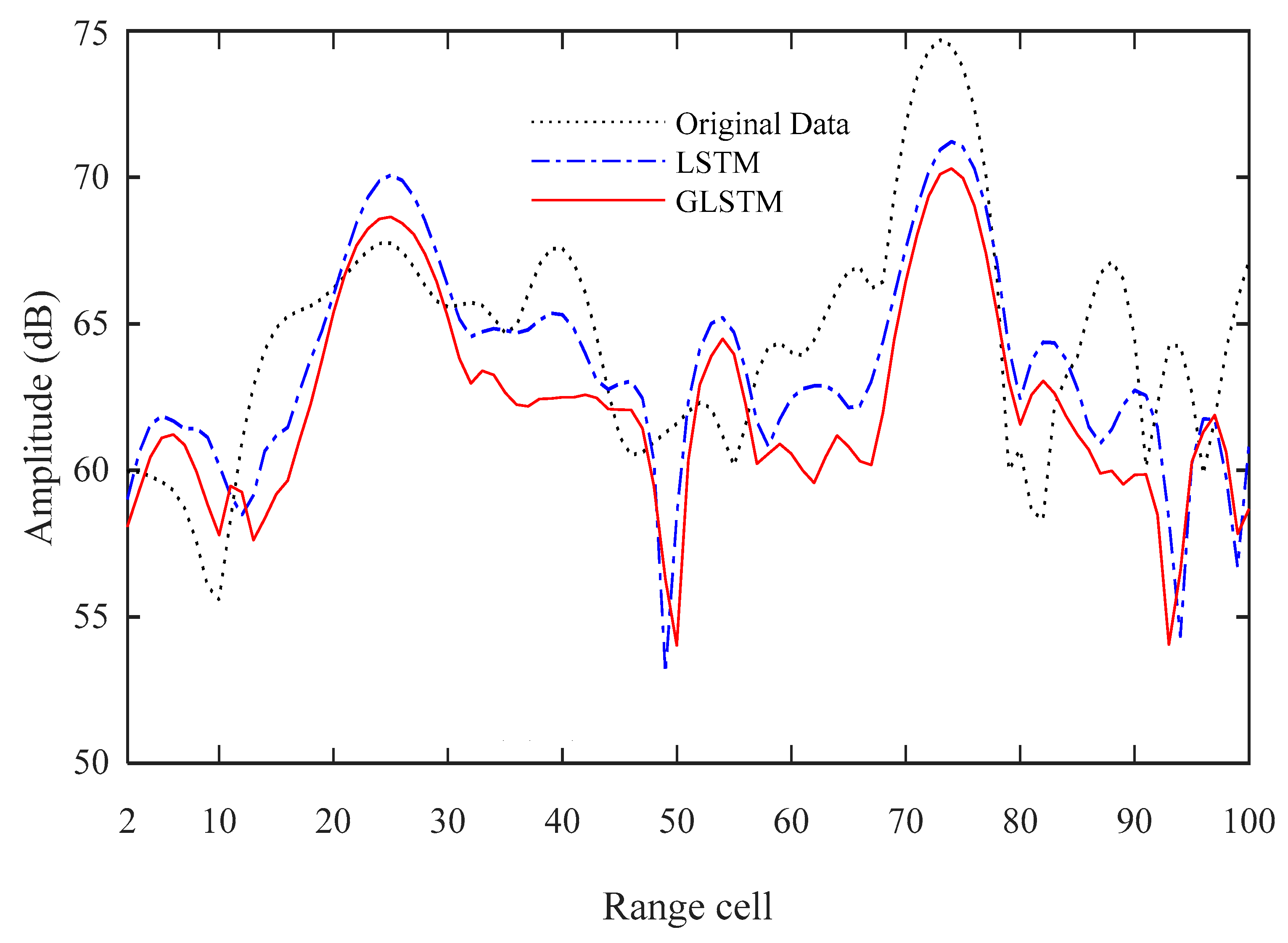
For data block II where targets exist, Figure 14 contrasts the result curves of the 2204th pulse. In comparison with Figure 13, the presented GLSTM-based method not only effectively suppresses sea clutter but also exhibits improved preservation of the target signal.
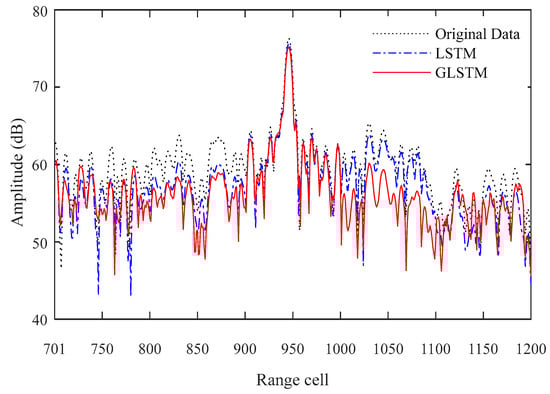
Figure 14.
The sea clutter suppressed result for data block II in the 2204th pulse.
According to the aforementioned results, the proposed GLSTM-based method has better sea clutter suppression performance than the LSTM-based method.
4.5. Analysis
In order to demonstrate the performance of the proposed method, some supplementary experiments are carried out in this section.
4.5.1. Robustness Analysis
For better evaluation of the performance of the proposed GLSTM-based method, Figure 15, Figure 16 and Figure 17 examine the robustness in preserving the target signal quality under different noise levels for data block II from the 701st to the 800th range cell. Gaussian white noise with different levels was added to the range-compressed domain of the radar echo. Then, the performance of the proposed GLSTM-based method was tested.
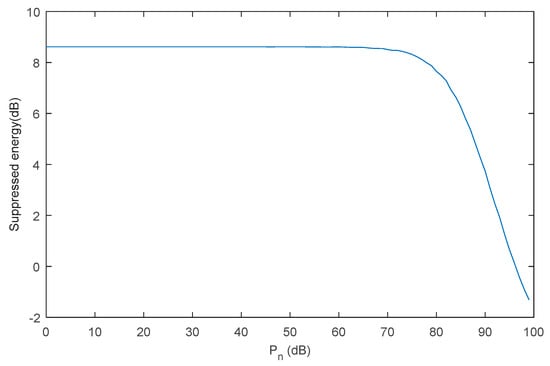
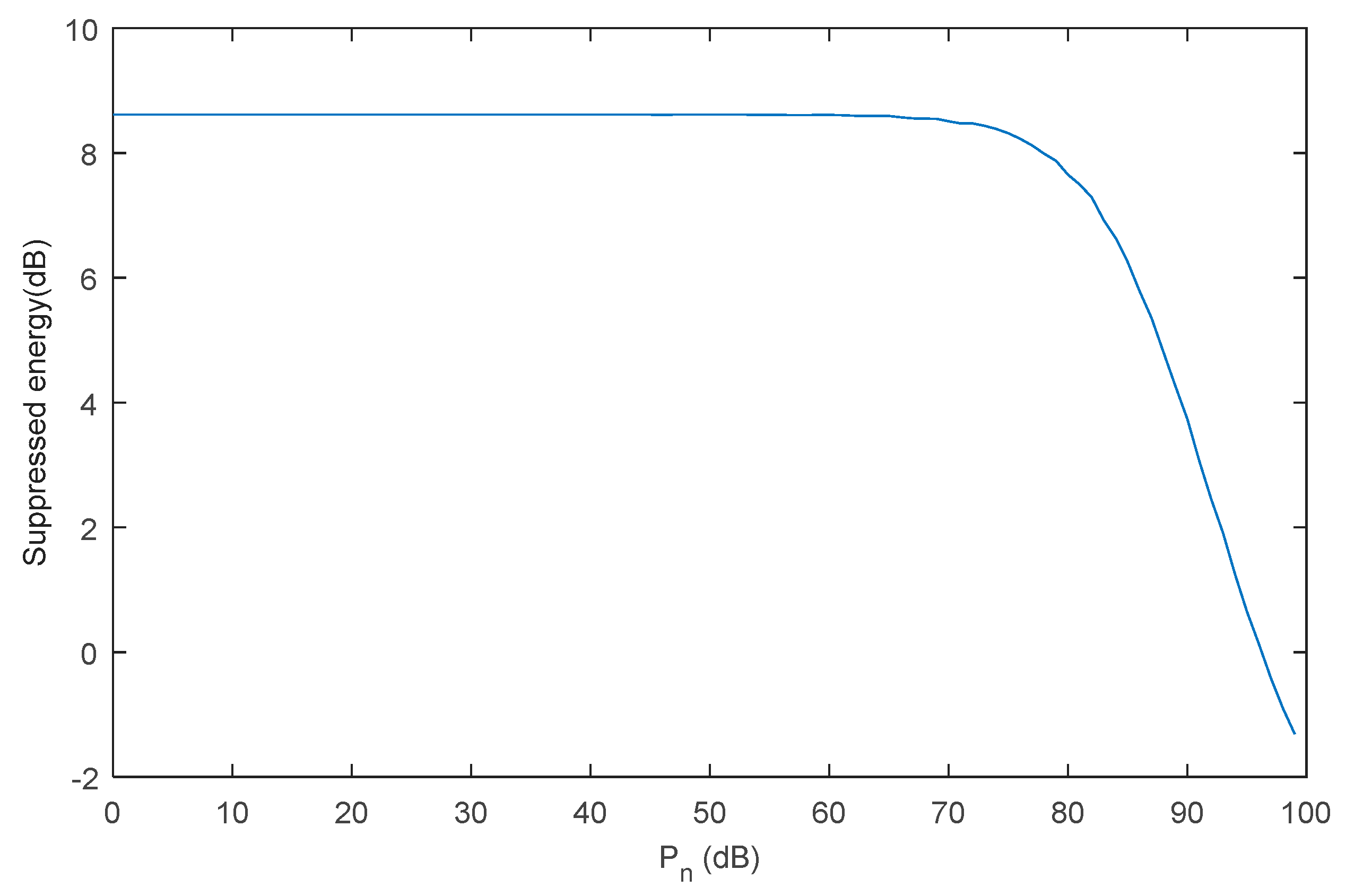
Figure 15.
The variation of suppressed energy with different noise levels.
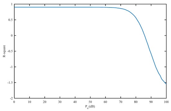
Figure 16.
The variation of R-square with different noise levels.
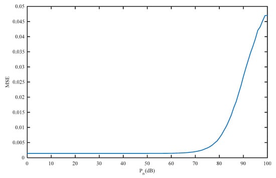
Figure 17.
The variation of MSE with different noise levels.
In Figure 15, Figure 16 and Figure 17, represents the added noise level of the input signal. represents the added noise at 0 dB.
Figure 15 shows the variation of suppressed energy with different noise levels. When the added noise is less than 60 dB, the suppression of the GLSTM-based method stabilizes at 8.6 dB. When the added noise is more than 60 dB, the sea clutter suppression performance is significantly reduced.
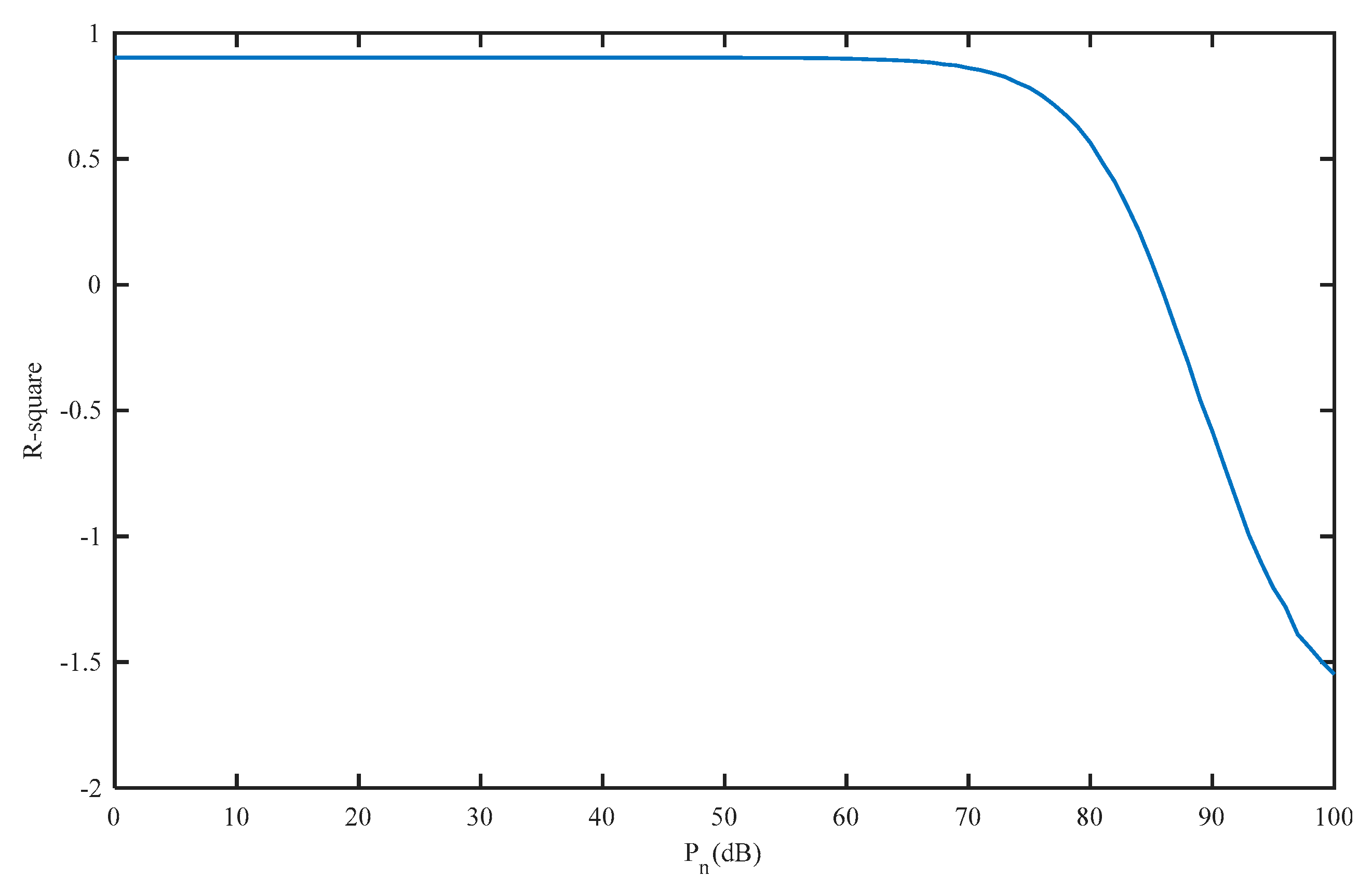
Figure 16 shows the variation of R-square with different noise levels. R-square is the average value of the 100 echo data. When the added noise is less than 60 dB, the output R-square of the GLSTM-based method stabilizes at 0.90. When the added noise is higher than 60 dB, the R-square curve rapidly drops off and the prediction accuracy of the proposed method significantly decreases.
Figure 17 shows the variation of the mean squared error (MSE) with different noise levels. MSE is the average value of the 100 echo data. When the added noise is less than 60 dB, the output MSE of the proposed method stabilizes at 0.0014. When the added noise is more than 60 dB, the R-square rapidly increases and the prediction accuracy of the proposed method significantly decreases.
The results of the experiments in Figure 15, Figure 16 and Figure 17 meet expectations and substantiate the robustness of the proposed method. When noise is in a certain range, the proposed method can resist the interference of noise. But when the noise is too large or even submerges the signal, the proposed method results in output errors.
4.5.2. Weak Targets Detection
The validity of the proposed method has been verified as mentioned before. In order to further illustrate the applicability of the proposed method for weak targets, a simulation experiment has been carried. In this experiment, the input is sea clutter data with different SCR values and the output is the suppressed sea clutter result using the proposed method.
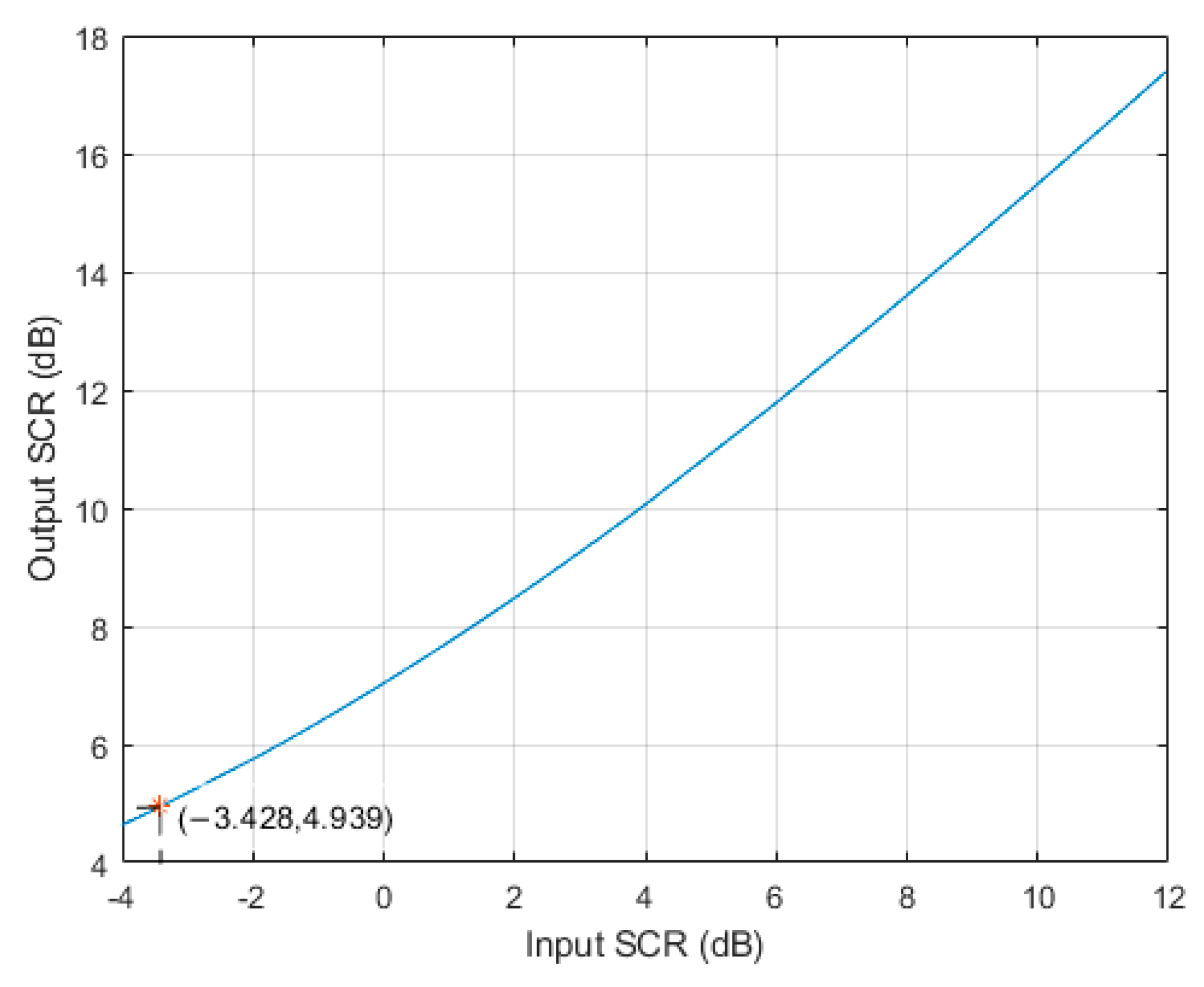
As shown in Figure 18, the output SCR of the proposed method is approximately linearly related to the input SCR of the proposed method. When the input SCR is −3.4 dB, the output SCR is 4.9 dB. This indicates that the proposed method is still valid for detecting weak targets.
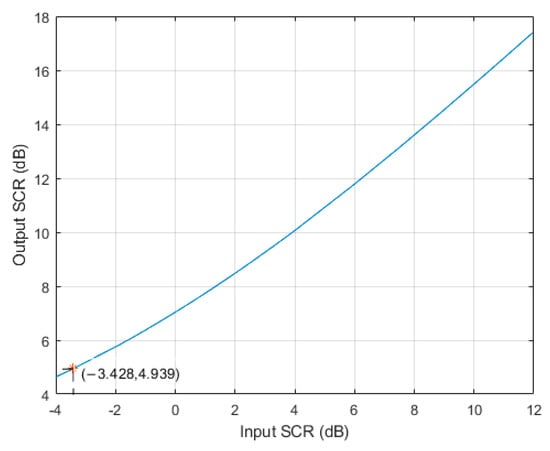
Figure 18.
The relationship between the input SCR and output SCR of the proposed method.
4.5.3. Comparison of Probability Densities
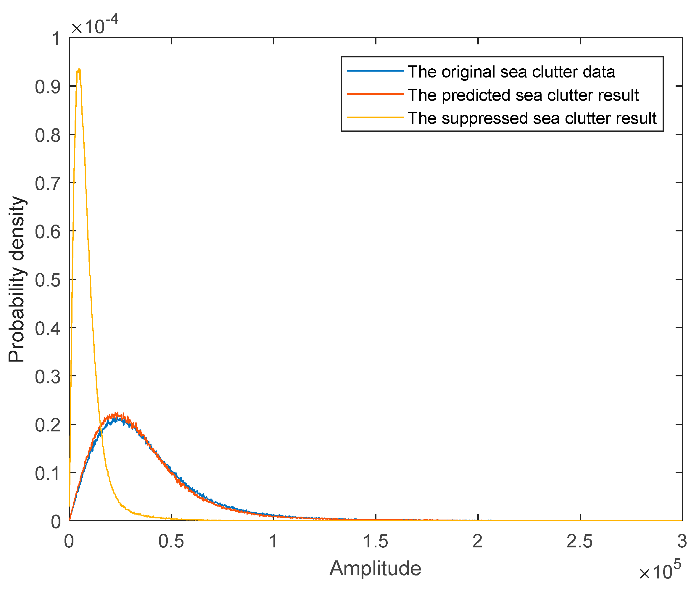
The PDF results of the original sea clutter data, the predicted sea clutter result, and the suppressed sea clutter result are shown in Figure 19. The PDF of the predicted result is close to that of the original sea clutter data, and the average difference between them is , which indicates that the proposed method can effectively predict the sea clutter data.
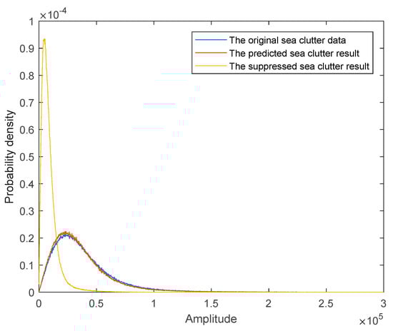
Figure 19.
The PDF results of the original sea clutter data, the predicted sea clutter result, and the suppressed sea clutter result.
Compared with the original sea clutter data, the position of the maximum probability density of the suppressed result is obviously shifted to the left along the horizontal coordinate, which indicates that the energy of the sea clutter is effectively suppressed by the proposed method.
4.5.4. Comparison of the Prediction Computation Efficiency
The calculation of the network was conducted using Intel(R) Core(TM) i7-8850H CPU (the base clock frequency is 2.60 GHz) and NVIDIA Quadro P3200 GPU. The built-in RAM is 64 GB. The comparison of the computation efficiency between the LSTM-based method and GLSTM-based method is shown in Table 1. The predicting duration of the GLSTM-based method is 57.75 s for sea clutter data with 100 range cells and 4380 pulses. The predicting duration of the LSTM-based method is 47.85 s for the same input data.

Table 1.
The Comparison of Computation Efficiency between the LSTM-based Method and GLSTM-based Method.
Although the duration of the proposed method is longer than that of the LSTM-based method, in the application of the methods, compared with the LSTM-based method, the GLSTM-based method achieves 2.3 dB improvement of the SCR at the cost of 10 s running time, which is worthwhile. The reason for the increase in duration is that the proposed method adds a GAN on the basis of the LSTM.
4.5.5. Applicability to Another Area with Different Wave Field Characteristics
In order to demonstrate the robustness of the proposed method, experiments on data with different radars and different scenarios were conducted.
The sea clutter suppression model was trained with the data of sea-detecting X-band experimental radar [19,20], which is located at the sea target detection test site in the coastal area of Yantai, Shandong province. The model was tested with the data of IPIX X-band polarimetric coherent radar [22,23], which is located on a cliff facing the Atlantic Ocean in Canada. Table 2 shows a comparison of the radar and wave field characteristics between the training and testing data.
Table 2.
A comparison of radar and wave field characteristics between the training and testing data.
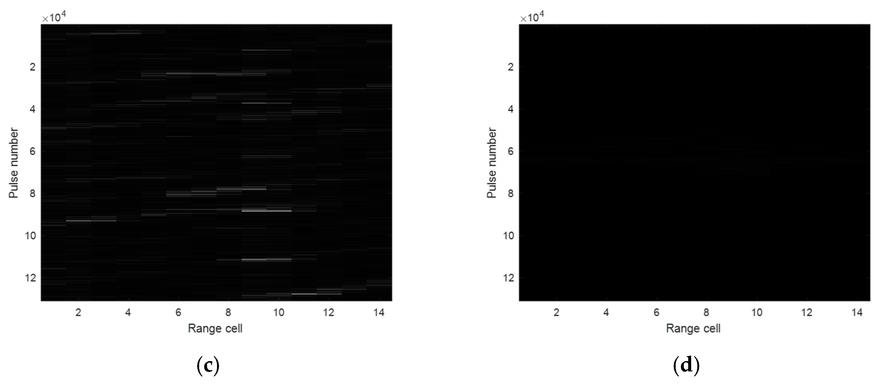
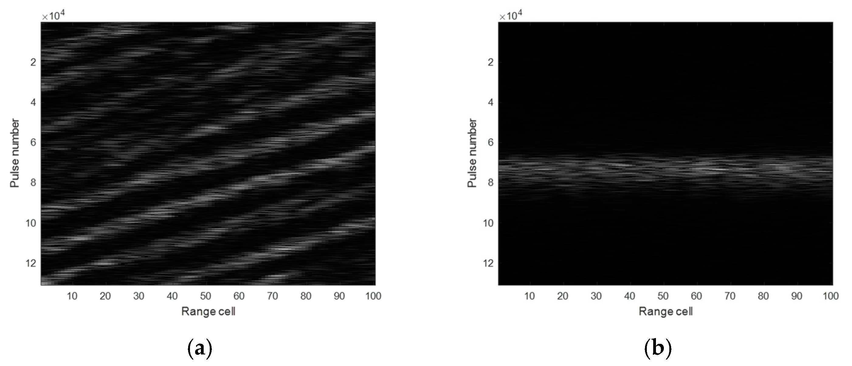
The results of the sea clutter suppression on the IPIX X-band polarimetric coherent radar data by the method trained on X-band experimental radar data are shown in the Figure 20. The energy of sea clutter is suppressed by 14.8 dB on average. The results show that the proposed method is applicable to another area with different wave field characteristics from the training data.
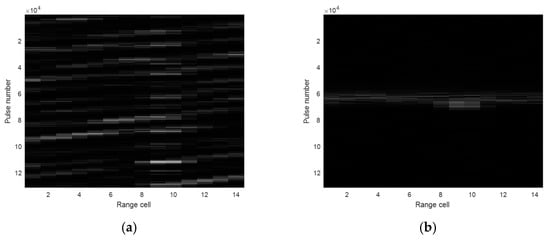

Figure 20.
Sea clutter suppression results of IPIX X-band polarimetric coherent radar data. (a) The original signal in the range compression domain. (b) The original imaging result. (c) The sea clutter suppressed result in the range compression domain. (d) The sea clutter suppressed result in the imaging domain.
4.5.6. Applicability to Different Sea States
The proposed method is applicable to another area with different sea state levels in the training data. In order to verify the robustness of the proposed method under different sea states, experiments are conducted on data with different sea states. As listed in Table 3, the model was trained with the training data from sea state 4 and tested in sea state 5 and sea state 3.
Table 3.
The parameters of training data and testing data with different sea states.
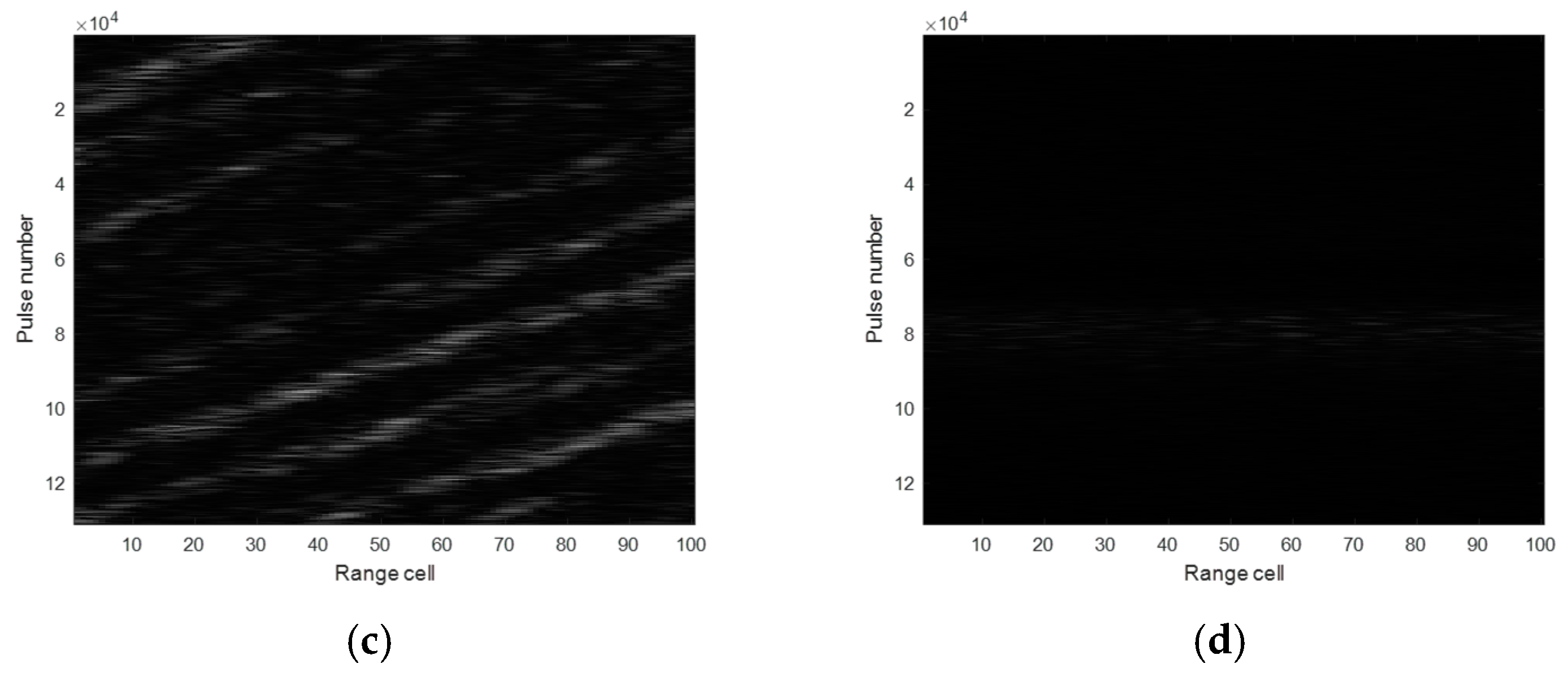
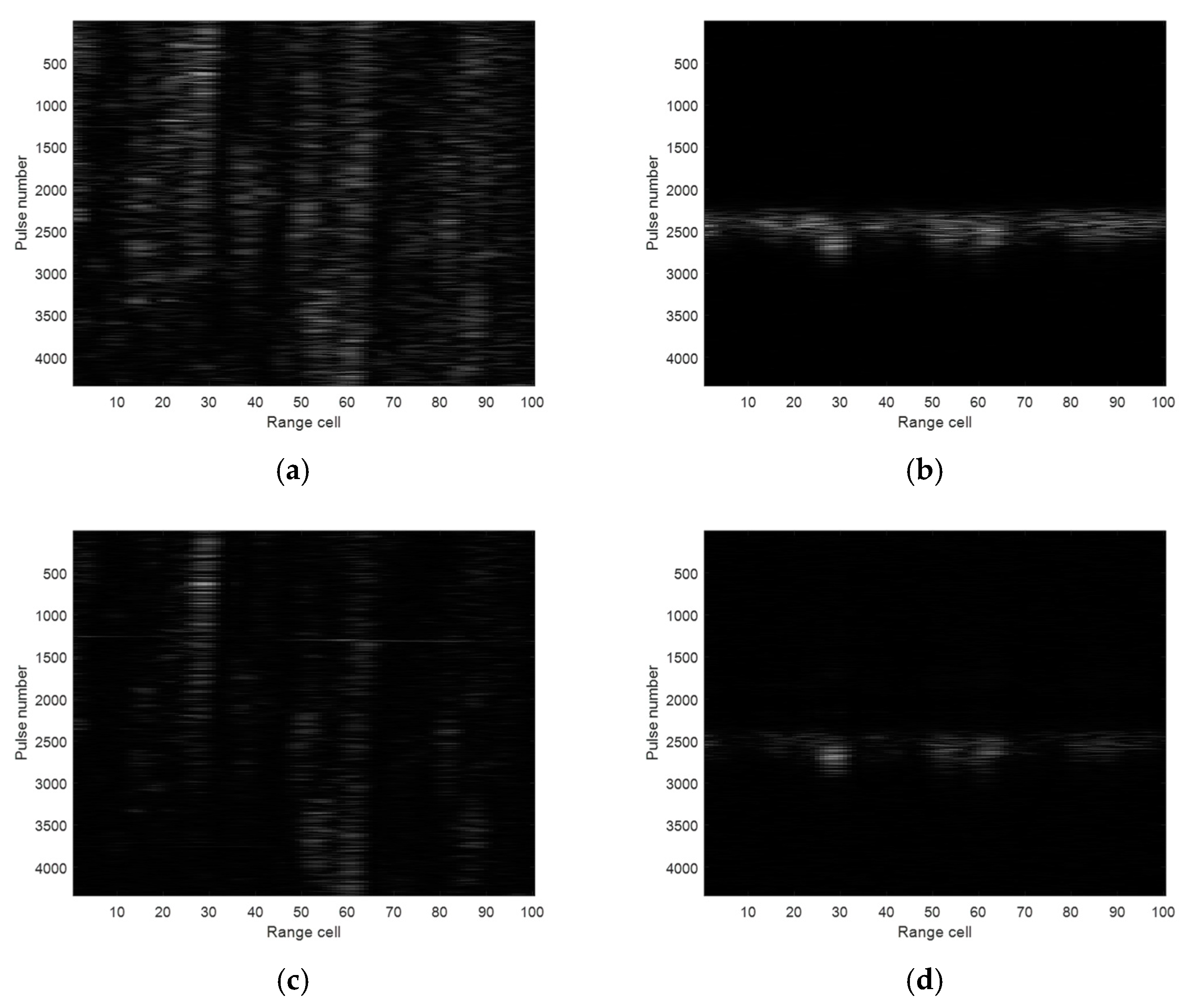
The sea clutter suppression results of the testing data with sea state 5 are shown in Figure 21. The energy of sea clutter is suppressed by 6.2 dB on average. The sea clutter suppression results of the testing data with sea state 3 are shown in Figure 22. The energy of the sea clutter is suppressed by 5.7 dB on average.


Figure 21.
Sea clutter suppression results of the data with sea state 5. (a) The original signal in the range compression domain. (b) The original imaging result. (c) The sea clutter suppressed result in the range compression domain. (d) The sea clutter suppressed result in the imaging domain.
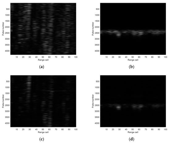
Figure 22.
Sea clutter suppression results of data with sea state 3. (a) The original signal in the range compression domain. (b) The original imaging result. (c) The sea clutter suppressed result in the range compression domain. (d) The sea clutter suppressed result in the imaging domain.
4.5.7. The Effect of White Caps
White caps have little effect on training. The performance of the sea clutter suppression is still significant regardless of whether the white caps participate in the training data.
A set of comparison experiments were conducted to illustrate this problem. The model was trained using different range cell data in the same set of sea clutter data, which is shown in Figure 23a. One experiment trained the model using the 74th range cell, where white caps obviously exist. Another experiment trained the model using the 1st range cell, where white caps were relatively insignificant.
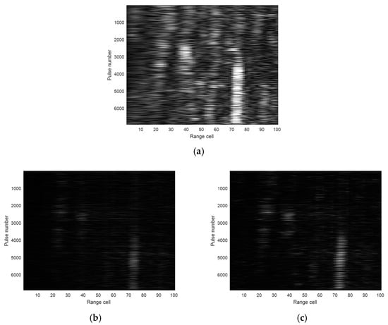
Figure 23.
The effect of white caps on training. (a) Original sea clutter signal in range compression domain. (b) Sea clutter suppressed result obtained by the model trained in the 74th range cell data. (c) Sea clutter suppressed result obtained by the model trained in the 1st range cell data.
Figure 23 shows the sea clutter suppression results processed by the model trained with different range cell data. For the model trained with range cell data where white caps obviously exist, the energy of the sea clutter is suppressed by 13.7 dB on average, which is shown in Figure 23b. For the model trained with range cell data where white caps are relatively insignificant, the energy of the sea clutter is suppressed by 11.8 dB on average, which is shown in Figure 23c. These results show that the selected training data have little effect on the sea clutter suppression performance of the proposed method.
4.5.8. Applicability to Wind Seas and Swell Dominant Seas
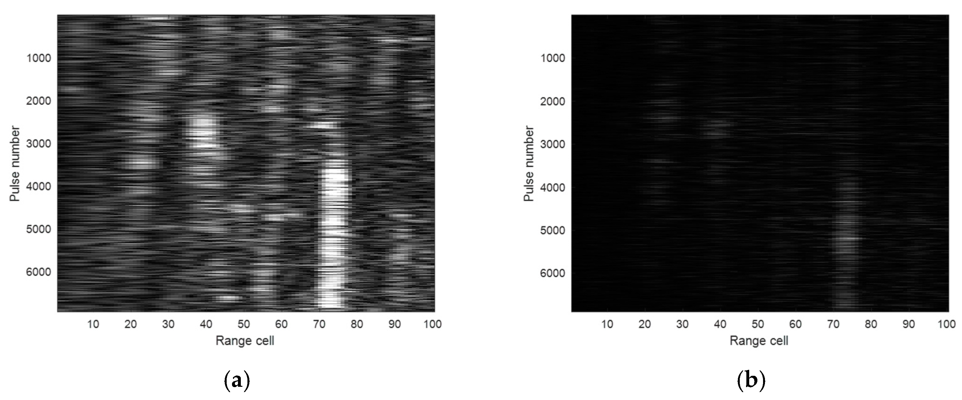
The proposed method can work well in both wind seas and swell dominant seas, as shown in Figure 24 and Figure 25, respectively. The data were obtained by the same radar observing the same area of sea at different times. The radar works in staring mode. The data corresponding to Figure 24 were obtained from the azimuth of 42.17 degrees, and the data corresponding to Figure 25 were obtained from the azimuth of 9.62 degrees.
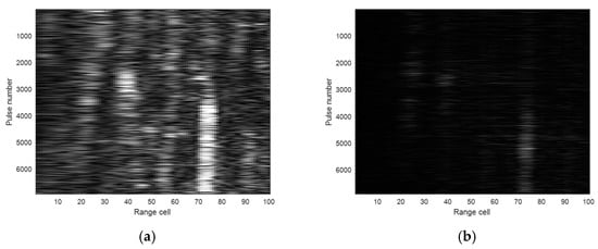
Figure 24.
The sea clutter suppressed the result of wind seas data. (a) The original data. (b) The sea clutter suppressed result.

Figure 25.
The sea clutter suppressed the result of swell dominant seas data. (a) The original data. (b) The sea clutter suppressed result.
5. Conclusions
A novel sea clutter suppression method combining generator and LSTM networks is proposed in this paper. The experimental results illustrated that the proposed method outperformed the LSTM-based method in sea clutter suppression. The proposed method is applicable to radar data and synthetic aperture radar (SAR) data. For example, it can be utilized to improve the accuracy of parameter estimation in SAR imaging of maneuvering ships.
Of course, the algorithm still has the possibility of further improvement:
- This proposed method uses a deep learning network for predicting sea clutter, subsequently suppressing the sea clutter through cancellation with the original echo. During training, it is essential to use sea clutter to construct the training dataset. In practical scenarios, radar echoes from real-world measurements without targets contain various interferences and noise, which reduces the accuracy of sea clutter prediction. In the future, reducing the sensitivity of the network to interference will be beneficial to enable the network to learn more intrinsic variations of sea clutter features, thus improving the accuracy of sea clutter prediction.
- The predicted sea clutter is used in the proposed method to cancel the echo. In a case where the echo contains a target, the energy of the target is inevitably attenuated after the cancellation. In the future, efforts to preserve the target energy as much as possible will be the key to improving the SCR and thus the radar’s target detection performance during the sea clutter suppression process.
Author Contributions
Conceptualization, J.Y. and Z.Y.; methodology, J.Y. and Z.Y.; software, J.Y., B.P. and H.Z.; validation, B.P.; formal analysis, J.Y. and B.P.; investigation, J.Y.; resources, J.Y.; data curation, J.Y. and B.P.; writing—original draft preparation, J.Y.; writing—review and editing, B.P. and H.Z.; visualization, J.Y., B.P., H.Z., H.L., C.L. and H.S.; supervision, Z.Y. All authors have read and agreed to the published version of the manuscript.
Funding
This work was supported in part by the National Natural Science Foundation of China under Grant 62271031 and in part by the National Key Lab Foundation of Microwave Imaging Technology.
Data Availability Statement
The data presented in this paper are available on request from the corresponding author.
Conflicts of Interest
The authors declare no conflicts of interest.
Abbreviations
The following abbreviations are used in this manuscript:
| SAR | SAR Synthetic Aperture Radar |
| LSTM | Long Short-Term Memory Networks |
| GANs | Generative Adversarial Networks |
| RBFNNs | Radial Basis Function Neural Networks |
| ANNs | Artificial Neural Networks |
| RNNs | Recurrent Neural Networks |
| GLSTM | modified prediction model combining the generator and LSTM |
| FC | fully connected layer |
| SCR | signal-to-clutter |
| JS | Jensen–Shannon |
| R-square | coefficient of determination |
| MSE | mean squared error |
References
- Haykin, S.; Li, X.B. Detection of signals in chaos. Proc. IEEE 1995, 83, 95–122. [Google Scholar] [CrossRef]
- Haykin, S.; Puthusserypady, S. Chaotic dynamics of sea clutter. Chaos Interdiscip. J. Nonlinear Sci. 1997, 7, 777–802. [Google Scholar] [CrossRef] [PubMed]
- Xie, N.; Leung, H.; Chan, H. A multiple-model prediction approach for sea clutter modeling. IEEE Trans. Geosci. Remote Sens. 2003, 41, 1491–1502. [Google Scholar]
- Wang, Q.; Wen, B. Active Learning Artificial Neural Networks Ensemble for HF Ground Wave Radar Sea Clutter Predicting. In Proceedings of the 2009 International Conference on Computational Intelligence and Software Engineering, Wuhan, China, 11–13 December 2009; pp. 1–4. [Google Scholar]
- Gao, Z.; Chen, L. Sea Clutter Sequences Regression Prediction Based on PSO-GRNN Method. In Proceedings of the 2015 8th International Symposium on Computational Intelligence and Design (ISCID), Hangzhou, China, 12–13 December 2015; Volume 1, pp. 72–75. [Google Scholar]
- Han, M.; Xi, J.H.; Xu, S.G.; Yin, F.L. Prediction of chaotic time series based on the recurrent predictor neural network. IEEE Trans. Signal Process. 2004, 52, 3409–3416. [Google Scholar] [CrossRef]
- Salehinejad, H.; Sankar, S.; Barfett, J.; Colak, E.; Valaee, S. Recent advances in recurrent neural networks. arXiv 2017, arXiv:1801.01078. [Google Scholar]
- Hochreiter, S.; Schmidhuber, J. Long short-term memory. Neural Comput. 1997, 9, 1735–1780. [Google Scholar] [CrossRef]
- Ma, L.; Wu, J.; Zhang, J.; Wu, Z.; Jeon, G.; Tan, M.; Zhang, Y. Sea Clutter Amplitude Prediction Using a Long Short-Term Memory Neural Network. Remote Sens. 2019, 11, 2826. [Google Scholar] [CrossRef]
- Yu, Y.; Si, X.; Hu, C.; Zhang, J. A review of recurrent neural networks: LSTM cells and network architectures. Neural Comput. 2019, 31, 1235–1270. [Google Scholar] [CrossRef] [PubMed]
- Goodfellow, I.; Pouget-Abadie, J.; Mirza, M.; Xu, B.; Warde-Farley, D.; Ozair, S.; Courville, A.; Bengio, Y. Generative Adversarial Nets. Adv. Neural Inf. Process. Syst. 2014, 27, 2672–2680. [Google Scholar]
- Li, C.L.; Chang, W.C.; Cheng, Y.; Yang, Y.; Póczos, B. Mmd gan: Towards deeper understanding of moment matching network. Adv. Neural Inf. Process. Syst. 2017, 30. [Google Scholar]
- Durgadevi, M. Generative adversarial network (gan): A general review on different variants of gan and applications. In Proceedings of the 2021 6th International Conference on Communication and Electronics Systems (ICCES), Coimbatore, Indian, 8–10 July 2021; pp. 1–8. [Google Scholar]
- Takens, F. Detecting Strange Attractors in Turbulence; Dynamical Systems and Turbulence, Warwick 1980: Proceedings of a Symposium Held at the University of Warwick 1979/80; Springer: Berlin/Heidelberg, Germany, 2006; pp. 366–381. [Google Scholar]
- Matsumoto, T.; Nakajima, Y.; Saito, M.; Sugi, J.; Hamagishi, H. Reconstructions and predictions of nonlinear dynamical systems: A hierarchical Bayesian approach. IEEE Trans. Signal Process. 2001, 49, 2138–2155. [Google Scholar] [CrossRef]
- Tsai, S.-C.; Tzeng, W.-G.; Wu, H.-L. On the Jensen-Shannon divergence and variational distance. IEEE Trans. Inf. Theory 2005, 51, 3333–3336. [Google Scholar] [CrossRef]
- Zhu, H.L.; Yu, Z.; Yu, J.D. Sea Clutter Suppression Based on Complex-Valued Neural Networks Optimized by PSD. IEEE J. Sel. Top. Appl. Earth Obs. Remote Sens. 2022, 15, 9821–9828. [Google Scholar] [CrossRef]
- Cao, L. Practical method for determining the minimum embedding dimension of a scalar time series. Phys. D Nonlinear Phenom. 1997, 110, 43–50. [Google Scholar] [CrossRef]
- Liu, N.; Dong, Y.; Wang, G.; Ding, H.; Huang, Y.; Guan, J.; Chen, X.; He, Y. Sea detecting X-band radar and data acquisition program. J. Radars 2019, 8, 656–667. [Google Scholar]
- Liu, N.; Ding, H.; Huang, Y.; Dong, Y.; Wang, G.; Dong, K. Annual Progress of Sea-detecting X-band Radar and Data Acquisition Program. J. Radars 2021, 10, 173–182. [Google Scholar]
- Rousson, V.; Goşoniu, N.F. An R-square coefficient based on final prediction error. Stat. Methodol. 2007, 4, 331–340. [Google Scholar] [CrossRef]
- Drosopoulos, A. Description of the OHGR Database; Tech. Note; National Defence Canada, Defence Research Establishment Ottawa: Ottawa, ON, Canada, 1994; pp. 1–30. [Google Scholar]
- Greco, M.; Stinco, P.; Gini, F.; Rangaswamy, M. Impact of Sea Clutter Nonstationarity on Disturbance Covariance Matrix Estimation and CFAR Detector Performance. IEEE Trans. Aerosp. Electron. Syst. 2010, 46, 1502–1513. [Google Scholar] [CrossRef]


Disclaimer/Publisher’s Note: The statements, opinions and data contained in all publications are solely those of the individual author(s) and contributor(s) and not of MDPI and/or the editor(s). MDPI and/or the editor(s) disclaim responsibility for any injury to people or property resulting from any ideas, methods, instructions or products referred to in the content. |
© 2024 by the authors. Licensee MDPI, Basel, Switzerland. This article is an open access article distributed under the terms and conditions of the Creative Commons Attribution (CC BY) license (https://creativecommons.org/licenses/by/4.0/).