1. Introduction
For millions of years, the unrelenting power of erosion has carved and sculpted the world. It stimulates soil formation, shapes geological features, influences sediment transportation, and initiates carbon storage. However, erosion also threatens ecosystems, reduces agricultural production, and overall represents a loss of a non-renewable resource. In fact, erosion has been noted as the largest widespread threat to the environment [
1,
2]. In particular, soil erosion causes 75 billion metric tons of soil to be displaced each year around the world [
3]. Due to anthropogenic activities, rain events now pose an increased risk of irreparable soil erosion. As such, it is imperative to identify hotspots of erosion caused by rain events, allowing targeted mitigation strategies to be implemented.
A significant portion of Australia’s soil is old and weathered, leaving it vulnerable to erosion, something that significantly impacts Australia’s
$90 Billion agricultural industry [
4,
5]. Studies have found that a 10 cm loss of soil could result in an
$18 billion dollar impact on the industry [
6,
7,
8]. Additionally, erosion affects the quality of surrounding waterways. The increased turbidity from suspended soil particles can block sunlight from reaching the river bed, while nitrogen and phosphorus found in some soils can cause eutrophication [
9,
10]. Together, these can decimate river ecosystems, which are the lifeblood of outback Australia [
11]. Soil erosion and deposition can also alter the natural flow of water, causing flooding in areas that would not normally receive water while leaving others dry. Through these limited examples, it is clear the significant impact erosion can cause and why it needs to be closely monitored.
Despite its detrimental effects, the identification and monitoring of erosion is an arduous practice, particularly at large scales. The current erosion identification/monitoring techniques can be split into two categories, namely, predictive models and observational erosion analysis. Predictive models use erosion risk factors like slope, rainfall intensity, and land cover, to try and predict where erosion is likely to occur in an area [
12]. The most popular predictive model is the Revised Universal Soil Loss Equation (RUSLE) developed by the United States Department of Agriculture, which was released to the public in 1992 [
13]. Other studies have been completed using various predictive models ranging from looking at the multispectral signal of eroded areas to using land classification indexes to find gullies [
14,
15,
16,
17]. These models, like all other predictive models, are great for informing policy on a large scale but do not help accurately map erosion as it happens. This can only be completed using observational techniques, which are any processes where actual erosion is measured. Some examples of this are field studies and satellite data [
18]. Field studies involve looking for evidence of erosion or using erosion plots to determine impacts in a small area. These studies are expensive and labour-intensive whilst only gaining data for a small area [
19]. Satellite images can also be used by comparing different epochs to find any changes on the ground. Again, this method involves a large amount of human data interpretation and often does not reveal the full degree of erosion. More recently, a new technique of erosion analysis has been developed using Synthetic Aperture Radar (SAR) images to complete a CCD study [
20].
Synthetic Aperture Radar (SAR) is a satellite observation technique that can observe changes in the earth’s surface [
21]. SAR sensors emit radar waves towards the earth, measuring the intensity and phase difference in the backscattered wave. When readings from two different epochs are compared, changes in the earth’s surface can be identified [
22]. When comparing SAR images from different epochs, coherence is used to assess the correlation between backscatter signals, highlighting areas where the backscattering changes. Equation (1) is used to calculate coherence [
23].
where
and
are the complex pixel values of each of the SAR images and the angular brackets represent ensemble averaging. Using this equation results in a value from 0 to 1, with 1 being a strong correlation between the two epochs and 0 being no correlation. The factors that contribute to correlation can be split into four categories, being geometric, volumetric, thermal, and temporal [
23,
24,
25].
The geometric factor refers to the distance between the satellite’s position at each epoch, known as the baseline. Any value greater than zero will create additional decorrelation; however, values of less than a few hundred metres result in an insignificant effect [
25,
26]. Volumetric decorrelation is the most common and occurs when radar waves bounce off multiple surfaces before returning to the satellite. This is often caused by vegetation but can also be the result of soil moisture, buildings, gullies, and other influences [
27]. As long as there have been no changes in these factors between the two epochs, extra decorrelation should not occur. The third factor is thermal and is largely due to random errors of the receiver and, as such, cannot be easily adjusted for [
24]. The last factor is temporal; changes due to temporal factors are often what studies are examining, looking for any changes in the ground surface between epochs. This is where the change detection part is established. Using coherence values between pairs and comparing these values to other pairs, the temporal effects on decorrelation can be studied. This allows for changes in the ground surface structure to be highlighted at particular periods of time.
CCD is particularly useful for finding erosion as it can be used in all weather conditions over large areas, has a sizable amount of historical data, and can detect small changes in surface structure. As SAR is an active sensor, it can be used to detect changes through cloud cover and at any time of the day. This is extremely beneficial when trying to investigate rain events where cloud cover is likely. Many methods used to investigate erosion are limited in scope, only being possible in small areas, whilst remote-sensing techniques offer the ability to investigate the entire earth due to their space-borne nature and significant history of data. Lastly, when measuring erosion, CCD can measure small changes in the surface structure. This is due to the nature of backscattered waves. If the ground is disturbed, it will reflect a different signal than the previous epoch, allowing any such changes to be detected in a coherence image. One disadvantage of coherence is that some areas will always have a low coherence due to vegetation or gullies. However, this has been overcome by calculating the background coherence of an area and correcting for the impact of vegetation and gullies.
To the best of the authors’ knowledge, only a limited number of studies have been performed using CCD to measure erosion, with only one being completed in Australia [
28] and one other being used in Chile to measure erosion from rain events [
20]. These studies both used very different techniques. The study in Australia was completed by Castellazzi et al., 2023 [
28] and aimed at mapping gully erosion using CCD. It used a novel technique of creating large stacks using a small baseline subset (SBAS) method, creating a separate stack for dry and rainy conditions. Using this method, a large amount of data from the dry stack was used to estimate the background coherence, giving a highly accurate result. From this stack, the average and standard deviation for each pixel per temporal baseline were established. This is another advantage of the SBAS method as it allows a comparison between different temporal baselines. The background coherence was then used with the rain stack to highlight areas of erosion using a complex relationship between the two. Although using an SBAS method can give more accurate results, it also requires significant computer power and labour to complete the processing. As one proposed benefit of CCD is the reduced labour required, the need for computing power and human interaction with this method could be improved upon. The study from Chile completed by Cabré et al. (2020) [
20] uses a much simpler method.
Cabré et al. (2020) [
20] studied the erosion caused by a single rain event in the Atacama Desert using CCD. They used five coherence pairs with the same temporal baseline before the rain event to establish the average and standard deviation. They then determined the 95% confidence interval of each pixel and removed all values except the lower 2.5 percentile. Thus, this should only highlight areas that are very likely to have changed. The method used has a lower computational requirement; however. it did not validate its data successfully, only showing small areas that were examined during a field study.
This study aimed to refine the approach of previous work by proposing a method more rigorous than that used by Cabre et al. (2020) [
20], but not as computationally heavy as Castellazzi et al., 2023 [
28] and will provide a well-established validation of the results. This will be achieved by using fewer coherence pairs to estimate background coherence and correcting for still water and moisture changes while still utilising a streamlined approach.
3. Results
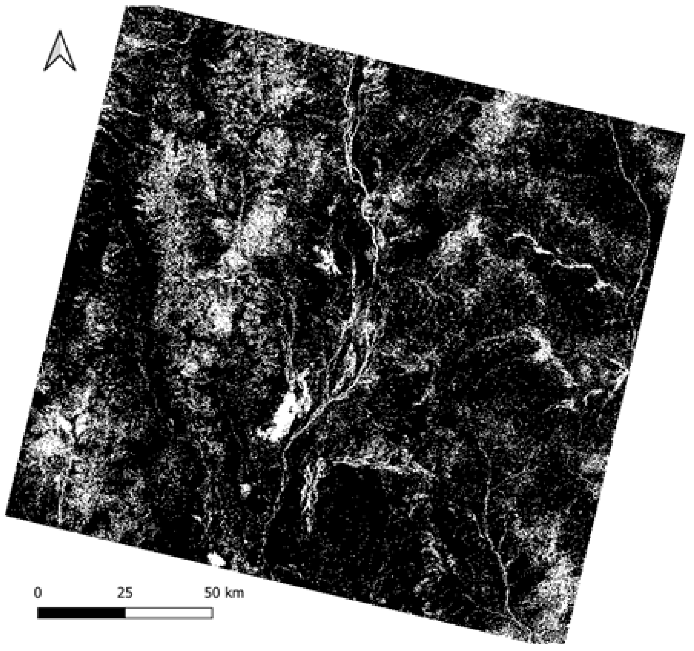
This study clearly demonstrated widespread erosion around the river system as a result of the rain event on 2 February 2022 as shown in
Figure 6. The speckly nature of SAR was evident in this image; however, it did suggest some areas of likely erosion. A number of these areas were then explored more in-depth during the field investigation.
As seen in Equation (2), there are four factors that contribute to coherence, being geometric, volumetric, thermal, and temporal. To ensure the results seen are only erosion, all other factors need to be removed. The geometric factors relate to changes in the physical position of the satellite between images. As stated earlier, pairs that have baselines larger than a few hundred metres may suffer from added decorrelation. The largest baseline in this study was 148 m as seen in
Table S2 (Supplementary Materials). As such geometric factors should not be contributing towards coherence changes [
25].
Next, the volumetric factors were explored. In this study, the most likely volumetric factors would be vegetation, soil moisture changes, and water. An assessment of the vegetation is shown in
Figure 7. It can be seen there was only a small amount of vegetation change between the first and second SAR images. The most notable difference between the images occurs in the rivers where water is lying in the second image causing the pixels to become whiter. Normally, vegetation growth in arid and semi-arid environments tends to occur 1–2 months after rainfall [
37,
38]. As the temporal baseline between images is 12 days, the difference in vegetation cover should be relatively small. As such, vegetation should not create a difference in coherence.
Soil moisture changes were examined in two ways, first using the Soil Moisture Active Passive (SMAP) mission and, secondly, using coherence pairs over longer temporal baselines.
Figure 8 shows the difference between values gained from the SMAP mission L3_SM_P_E product on 27 January 2022 and 7 February 2022. This SMAP product has a spatial resolution of 9 km and, as such, can only be used to provide an approximate assessment of changes in soil moisture.
As indicated in
Figure 8, there has been a small increase in soil moisture; however, this increase is not considered significant. The SMAP mission has an accuracy of 0.04 m
3/m
3 [
39], and as the largest difference in the study area is 0.053 m
3/m
3, it is only slightly higher than the accuracy of the equipment and, as such, is not considered a significant change.
To assess the moisture changes at a higher resolution, coherence pairs with different temporal baselines were investigated (
Figure 9). If soil moisture was affecting the coherence signal, it would be expected that there would be an increase in coherence in some areas as soil moisture dissipated. This cannot be seen in
Figure 9 as the coherence values decrease with time, with the average percentage difference between
Figure 9a and d being −9.3%. This is what would normally be expected from longer temporal baselines. This same comparison was made in
Figure 10 but over a dry period. Here, the average percentage difference was −5.2%, with a big portion begin concentrated in one area. This shows that there was a higher-than-normal decrease in coherence following the rain event, likely because of increased vegetation growth. This also shows that there were no increases in coherence due to soil moisture. Although these two data sources show that soil moisture should not have affected the study, soil moisture was still corrected as part of the method.
Lastly, laying water needs to be considered. Like most satellite data, SAR images cannot penetrate water bodies easily and, as such, in areas that may have still water, coherence values will be greatly affected. This factor was removed while processing as any areas with laying water were masked out.
The last factor to correct is the thermal factors. These factors are largely due to the limitations of the sensor, the atmospheric effects, and the randomness in any dataset [
24]. Thermal factors cannot be easily corrected, so in this study, they have been limited by averaging pairs to create a dry stack and then utilising this stack to apply spatial filtering. These solutions do not totally remove all effects, as seen by the noisy nature of the final product. Through careful interpretation of the results, this factor did not contribute to large coherence changes. With all other factors largely removed from the dataset, it was assessed that the only remaining cause for coherence loss could be attributed to temporal factors. For this study, the possible temporal factors were all related to changes in the surface structure, either by natural or anthropogenic processes. Due to the remoteness of the study area, it can be assumed that direct anthropogenic effects would be very low. As such, it can be concluded that any effects seen in the final data are effects of natural processes. As there was a large amount of rainfall in the study area over the 12 days that covered these analyses, it can be assumed that most of the natural changes would be due to water erosion. However, in the data, some effects from wildlife are present.
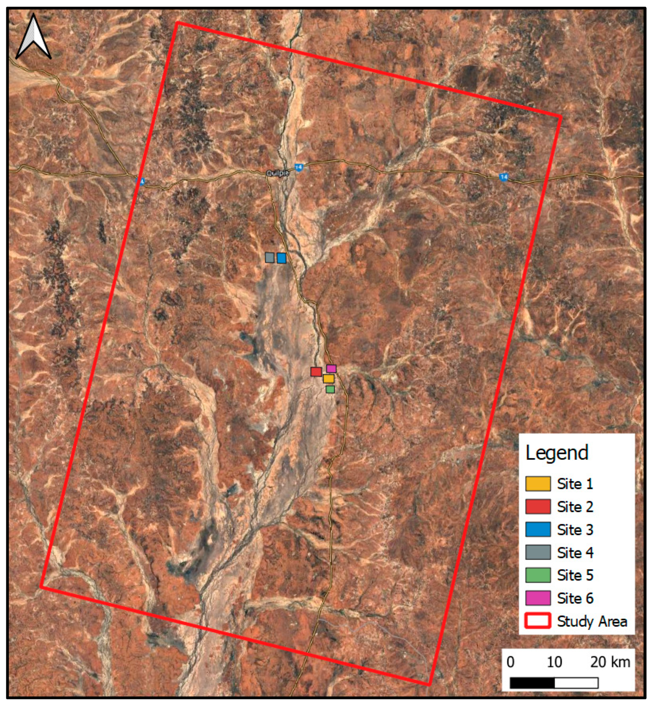
The data collected from the field campaign can assist in interpreting the outcome of the SAR data processing. In total, six sites were visited, with four drone surveys and four soil samples being completed. These sites can be seen in
Table 5 and are shown in
Figure 5.
Figure 11,
Figures S1 and S2 show the four drone surveys with the erosion results overlayed. Some conclusions about the accuracy of the data can be drawn from these results; however, it is difficult with erosion to pinpoint newly eroded areas from past erosion. As erosion does not occur uniformly over a site, areas where erosion was determined in the images may not have eroded during the rain event on 2 February 2022. As such, these images can be used as a guide only to help validate the possible location of erosion.
Figure 11a shows the results gained mostly coincide with erosion seen on the ground. Importantly, the data appears to suggest that erosion is occurring towards the end of the gullies, which is consistent with the natural formation of erosion. This is best seen in the detailed view in
Figure 11a. The area contained within the red square can be seen in
Figure 12. This area has obvious newly formed erosion.
Figure 13 shows the two sites that were visited but no drone survey was undertaken. These sites were likely highlighted due to a combination of soil moisture changes and changes in the surface like flattened grass and disturbed rocks. It is obvious that little or no erosion had occurred in these areas largely due to their flatness. Water moving through this area would have a very low flow rate and, as such, would struggle to cause erosion.
Figure 11b also highlights the need for continued improvement of this technique as it is obvious that some areas identified are likely soil moisture changes in the flat ground rather than erosion.
The shear strength of the soil from each of the drone flight areas can be seen in
Table 6. Using the typical shear strength values from the GeotechniCal Reference Package by the University of West England, soft soil is rated as 20–40 kPa [
40]. Each of the soil samples comfortably fit into this category, which is the second lowest possible strength category. This shows the weakness of these soils, which translates into a higher susceptibility to erosion [
41].
In addition to the fieldwork, the temporal coherence variation was investigated as shown in
Figure 14. Here, it can be seen that the coherence of five areas over the course of 2022 was plotted against rainfall data. Here Tests 1, 2, and 3 correspond to Sites 3, 2, and 1, respectively.
It is evident from
Figure 14 that there is a correlation between coherence and rainfall, although this correlation is not strong. Test areas 1, 2, and 3 had an average correlation coefficient of 0.61 while the control areas had a correlation of 0.24. However, this is to be expected as rainfall is not a perfect determinant of erosion. During the first rain event, all test areas where erosion is likely to have occurred saw a steep decrease in coherence, which resulted in high Z values, which can be seen in
Table 4. This occurred while the two control areas remained largely unchanged. This same pattern occurs multiple times throughout the year.
It should be noted that even though Control 2 in
Figure 14 was within a high coherence area, it did decrease throughout September to November 2022, likely due to changes in soil moisture; however, the decrease is small compared to that of the eroded areas. Another notable anomaly is the large rain event on 13 March 2022 that did not create a loss of coherence. This can be explained in two ways. By examining
Figure 1b, during this rain event, the river levels were only slightly raised and did not reach the same heights as the 2 February rain event. Along with this, due to the large rain event that had occurred recently, any areas likely to easily erode would have already eroded. As such, experiencing lower erosion rates is expected.
Figure 14 shows that coherence does appear to match erosion patterns over the course of 2022.
4. Discussion
The results presented from this model have identified areas that are likely to have eroded during the 2 February 2022 rain event. However, although the results are promising, further improvement is required to fully remove the effects of soil moisture. This study represents a new method for generating such results; a method that has advantages over similar studies. This study uses only seven coherence pairs to calculate the background coherence, resulting in significantly fewer computation resources than the SBAS method similar to Castellazzi et al. [
28].
The approach utilised in this study used two vital corrections that had not been seen in previous studies, namely laying water and soil moisture corrections. The laying water correction was only required in areas that were prone to laying water such as in the channel country; however, the soil moisture correction is vital to all CCD analyses that revolve around rain. Castellazzi et al. [
28] attempted to account for soil moisture using the stacking of coherence pairs with different temporal baselines; however, this did not completely explain how this removes soil moisture. As a result, the authors found that only 6 of the 13 identified areas could be attributed to erosion. Therefore, using a dedicated soil moisture correction like in this study may improve these results and are important to the validity of this study.
Even when considering the use of soil moisture removal, the largest impact on the accuracy of the erosion identification was the changes in soil moisture. Due to the flatness of the study area, many areas are inundated with water when rain occurs that then accumulates in the soil. When using soil moisture indices like SMAP or the Normalized Difference Moisture Index (NDMI), only small changes in soil moisture are evident. However, it appears that these small changes have a significant effect on the backscattered radar waves. Even when correcting for soil moisture changes seen in these indices, areas that do not seem to have erosion and likely have just experienced soil moisture changes are identified. This effect is not widespread, and with the knowledge of its existence, the data can be interpreted to determine the areas with actual erosion. Along with soil moisture, some other limitations exist, with these being the impacts of vegetation and the resolution of the mission. The lack of vegetation in the study area helped contribute to the strength of the results; however, in areas with higher vegetation, some artifacts existed. If this method were to be replicated in a highly vegetated area, it may struggle to identify erosion. This could be alleviated by using SAR satellites with longer wavelengths.
Additionally, the resolution of the Sentinel-1 SAR sensor means that some small amounts of erosion may not be detected in the large pixels. Identifying the implications of this factor is difficult due to two aspects. On the one hand, the effect of this factor is small as any changes to the surface structure do impact the intensity of the backscattered wave. On the other hand, small changes could be missed as they would be assumed to be noise. Even when considering these limitations, the method employed in this study is still widely usable.
Future studies should aim to better understand the effects of soil moisture on coherence values and attempt to find better ways for removing soil moisture content. This may be achieved using other sensors to measure soil moisture or by utilising a machine learning program to remove any defects. Such a process would create a more accurate representation of erosion.


