Assessing Satellite-Derived OpenET Platform Evapotranspiration of Mature Pecan Orchard in the Mesilla Valley, New Mexico

Abstract

Pecan is a major crop in the Mesilla Valley, New Mexico. Due to prolonged droughts, growers face challenges related to water shortages. Therefore, irrigation management is crucial for farmers. Advancements in satellite-derived evapotranspiration (ET) models and accessibility to data from web-based platforms like OpenET provide farmers with new tools to improve crop irrigation management. This study evaluates the evapotranspiration (ET) of a mature pecan orchard using OpenET platform data generated by six satellite-based models and their ensemble. The ET values obtained from the platform were compared with the ET values obtained from the eddy covariance (ETec) method from 2017 to 2021. The six models assessed included Google Earth Engine implementation of the Surface Energy Balance Algorithm for Land (geeSEBAL), Google Earth Engine implemonthsmentation of the Mapping Evapotranspiration at High Resolution with Internalized Calibration (eeMETRIC) model, Operational Simplified Surface Energy Balance (SSEBop), Satellite Irrigation Management Support (SIMS), Priestley–Taylor Jet Propulsion Laboratory (PT-JPL), and Atmosphere–Land Exchange Inverse and associated flux disaggregation technique (ALEXI/DisALEXI). The average growing season ET of mature pecan estimated from April to October of 2017 to 2021 by geeSEBAL, eeMETRIC, SSEBop, SIMS, PT-JPL, ALEXI/DisALEXI, and the ensemble were 1061, 1230, 1232, 1176, 1040, 1016, and 1130 mm, respectively, and 1108 mm by ETec. Overall, the ensemble model-based monthly ET of mature pecan during the growing season was relatively close to the ETec (R² of 0.9477) with a 2% mean relative difference (MRD) and standard error of estimate (SEE) of 15 mm/month for the five years (N = 60 months). The high agreement of the OpenET ensemble of the six satellite-derived models’ estimates of mature pecan ET with the ETec demonstrates the utility of this promising approach to enhance the reliability of remote sensing-based ET data for agricultural and water resource management.

1. Introduction

The Mesilla Valley in the south-central part of New Mexico is well-known for its agriculture due to its fertile soil and available irrigation water. Several crops are grown in the Mesilla Valley, including pecan, alfalfa, cotton, chili, and onion. Pecan orchards are pivotal in New Mexico’s agricultural landscape, serving as the predominant crop and demanding the highest volume of irrigation water annually [1]. New Mexico, situated in the southwestern part of the USA’s semiarid environment, has established itself as the leading pecan producer in the nation. Pecan is one of the major contributors to New Mexico’s economy [2,3,4]. In 2018, New Mexico produced 91.1 million pounds of in-shell pecan nuts, surpassing Georgia and becoming the number-one producing state in the USA [1]. It should be noted that Hurricane Michael was the reason the Georgia crop was down significantly in 2018 and 2019—it had largely recovered from that by 2020. New Mexico has consistently been the second highest pecan-producing state in the USA since 2011, except for those two years (2018 and 2019) when Georgia production dropped below that of NM. A large percentage of the pecans produced in New Mexico come from the Mesilla Valley (~Doña Ana County). Approximately 70% of the bearing acres in the state are in Doña Ana County, and more than 70% of the pecans produced in the USA come from Doña Ana County [2]. The US Department of Agriculture (USDA)’s National Agricultural Statistics Service (NASS) Cropland Data Layer (CDL) [5] shows that pecan acreage in the Mesilla Valley has expanded from 8778 ha in 2012 to 14,696 ha in 2021, a 67.4% increase. This expansion has increased irrigation demands and total crop water consumption in this river basin.

The Mesilla Valley’s topography features flat terrain that gradually slopes upwards to an elevation of 1524 m above the average sea level. The Rio Grande (river) meanders through the valley and serves as the primary water source for irrigation. The river flows during the irrigation season, when water is released from Elephant Butte and Caballo reservoirs on the Rio Grande, about 60 km north of the Mesilla Valley. Groundwater serves as a secondary source of irrigation water during periods of drought, when water from the river is not available or not enough to meet crop irrigation needs. The amount of water needed for pecan orchards in New Mexico can vary significantly due to several factors, including soil type, land area, orchard age, stage of development, and pruning techniques [6,7,8]. According to the research conducted by Kallestad et al. [9], the ideal level of irrigation for optimal pecan production in the southwestern region of the United States lies between 1.9 and 2.5 m per year. However, the persistent drought with less than 250 mm of rainfall per year for several decades has posed a significant challenge for farmers in the area. As a result, there is an urgent need for advanced irrigation water management tools to conserve water for irrigation purposes and tackle the water scarcity issue in the region.

Accurate measurement of water usage by crops is crucial, as evapotranspiration (ET) is generally the largest agricultural water loss from hydrological and ecological systems. Accurate estimation of ET is important in irrigation scheduling, water allocation, crop modeling, water stress evaluation, water dynamics in wetlands, and measuring energy and moisture transfer between the earth’s surface and the atmosphere [10,11,12]. Several methods, including eddy covariance, lysimeter, and Bowen ratio measurements, have successfully been used to estimate crop ET at a farm scale and in combination with crop coefficient at a regional level. However, these techniques can be costly, time-intensive, and require specialized knowledge and care of instrumentation [13]. Thus, several methods have been developed for estimating ET using remote sensing (RS) imagery (a.k.a. data). These RS-based methods involve calculating ET as a residual of surface energy balance equations [14,15]. RS models have been widely applied in measuring ET [11,14,15,16,17,18,19,20,21,22,23,24,25,26,27,28,29,30]. These models utilize satellite imagery and employ diverse algorithms to estimate ET with precision and efficiency. The advancement of RS-based ET methods has paved the way for estimating ET on a spatial and temporal scale, overcoming the limitations of traditional measurement techniques such as soil moisture and tensiometer probes, weighing lysimeters, Bowen ratio, and eddy covariance. The usage of this technology has helped assess the amount of water consumed by crops and understand the dynamics of the water cycle in different areas.

Water resource management has increasingly become essential, especially with prolonged droughts that have created increased competition for fresh water. In recent decades, advancements in satellite-based ET estimation for estimating the consumptive use of water have led to increased interest in its application from farmers and water managers. However, RS-based ET estimation requires unique expertise. The development of the OpenET platform has created readily available and easy-to-access crop ET via the internet. This paper aims to assess ET on a temporal scale (monthly, seasonal, and annual) of mature pecan orchards in the Mesilla Valley, New Mexico, generated on the OpenET platform by six remote sensing models and their ensembled mean by comparing the results with measurements using the eddy covariance (EC) method from 2017 to 2021. Mature pecan orchards are considered here to be orchards with trees 20 years of age or older. The goal is to identify the best remote sensing model or ensemble for estimating the ET of mature pecan orchards at the farm scale. We hope that this assessment will aid farmers and water managers in using the OpenET platform to improve the management of irrigation water to grow pecan.

1.1. Description of OpenET Platform Models

The OpenET and Google Earth Engine Evapotranspiration Flux (EEFlux) platforms provide automated methods for calculating ET based on remote sensing data and give users access to ET for individual fields. OpenET (https://openetdata.org, accessed on 29 January 2022) combines algorithms from multiple remote sensing models using Landsat satellite data to produce ET at a spatial resolution of 30 m by 30 m using six satellite-based models and their ensemble. The available models within OpenET include Google Earth Engine implementation of the Surface Energy Balance Algorithm for Land (geeSEBAL) by Bastiaanssen et al. [16,17,18] and Laipelt et al. [24], Google Earth Engine implementation of the Mapping Evapotranspiration at High Resolution with Internalized Calibration (eeMETRIC) model by Allen et al. [14,15], Operational Simplified Surface Energy Balance (SSEBop) by Senay et al. [10,25], Satellite Irrigation Management Support (SIMS) by Melton et al. [26] and Pereira et al. [27], Priestley–Taylor Jet Propulsion Laboratory (PT-JPL) by Fisher et al. [28], Atmosphere–Land Exchange Inverse/Disaggregation of the Atmosphere–Land Exchange Inverse (ALEXI/DisALEXI) by Anderson et al. [22,23], and their ensemble. The OpenET program employs a range of gridded weather datasets derived from multiple weather stations covering the entire United States, such as gridMET [29], to determine grass reference ET (ET_o) and precipitation. Each model is described in the following sections.

1.2. geeSEBAL

The Surface Energy Balance Algorithm for Land (SEBAL) is a single-source remote sensing model developed by Bastiaanssen et al. [16,17,18]. The addition of “gee” in the name, geeSEBAL, represents implementing the SEBAL model on the Google Earth Engine. Multispectral, near-infrared, and thermal bands from satellite images are used to calculate SEBAL’s vegetation indices and land surface temperature. The model is based on energy balance (EB) at the predefined surface boundary, where latent heat flux (λET) is calculated as a residual of the EB. The net radiation (Rn) in the SEBAL model is calculated as the difference between the incoming and outgoing short- and long-wave radiations. The soil heat flux (G) is calculated as a ratio of the soil heat flux and Rn using an empirical equation [16,17,18] based on vegetation cover, surface temperature, and albedo. The sensible heat (H) is calculated using the bulk aerodynamic resistance function (r_ah) and near-surface temperature gradient (dT) through an iterative process considering the effects of atmospheric stability. The dT is calculated using a simple linear function between two near-surface heights $,{ z}_1$ and $z_2$, which is generally 0.1 and 2 m using wind speed extrapolated to some blending height above the ground surface of 200 m [14,15,16,17,18,30]. The SEBAL technique to estimate dT as an indexed function of radiometric surface temperature eliminates the need for accurate surface or air temperature measurements to calculate the surface’s sensible heat flux [14,15]. SEBAL applies a self-calibration procedure to train the surface energy balance by taking two “anchor” pixels as reference points [14,15,16,31]. The two anchor pixels are used to estimate the corresponding hot and cold near-surface temperatures (dT). At the time of the satellite overpass, the instantaneous ET is extrapolated to the daily ET using the evaporative fraction (Λ), computed as a ratio between the instantaneous values of λET and the available energy (Rn–G) for each pixel. It is assumed that Λ is constant throughout the day. This assumption, however, can underpredict the daily ET in warm, arid environments where afternoon advection or increased afternoon wind speeds may increase ET in proportion to Rn-G [14].

The SEBAL model has been validated with data obtained from the large-scale field experiments EFEDA (Spain), HAPEX-Sahel (Niger), and HEIFE (China) by Bastiaanssen et al. [30]. It has the advantage of estimating ET for large areas with minimal weather station data requirements [31]. Compared to other remote sensing models, the SEBAL model has been published widely in the literature [31,32,33,34,35,36,37]. In addition to the United States, the SEBAL model has been used in many countries, such as Egypt, India, Sri Lanka, Pakistan, and Argentina, to determine crop consumptive water use, crop water stress, and irrigation performance under various irrigation conditions [31]. Tasumi et al. [32] compared the SEBAL-estimated ET with the lysimeter-measured ET for crops in southern Idaho. The findings indicated that the predicted ET for monthly periods averaged ±16% compared to the lysimeter. Singh et al. [38] used the SEBAL model to estimate ET for drip-irrigated corn on a large scale in south-central Nebraska, USA. Their study compared the model crop ET results with field measurements of ET from the Bowen ratio energy balance system (BREBS). The study indicated a good correlation between the BREBS-measured and SEBAL-estimated ET, with an R² of 0.73 and a root mean square difference (RMSD) of 1.04 mm/day. Bezerra et al. [33] compared the SEBAL-estimated ET with the Bowen ratio measurements for a cotton field in Ceará State, Brazil. The findings showed a good correlation between measured and estimated ET, with an R² of 0.9 and a root mean square error (RMSE) of 0.4 mm/day. However, Mkhwanazi and Chávez [39] showed that the SEBAL model underestimated the ET of alfalfa by 5.7% to 45.5% with an average of 29% (n = 9 days of Landsat 7 ETM+ images) when compared to lysimeter measurements at the Colorado State University Arkansas Valley Research Center near Rocky Ford in eastern Colorado. They attributed the underestimation of ET to the SEBAL model’s deficiency in estimating H under advective conditions of high wind speeds, warm air, and drought.

1.3. eeMETRIC

The METRIC model [14,15] is a variant of the SEBAL model. It employs the same principles and techniques as SEBAL [14,15]. Adding “ee” in front of METRIC represents the implementation of the METRIC model on the Google Earth Engine. METRIC and SEBAL are both surface energy balance (EB) methods that use remotely sensed surface reflectance, near-infrared (NIR), and thermal bands (IR) to estimate ET as a residual of the energy balance equation [14,15,40]. The algorithms of these models, METRIC and SEBAL, estimate ET fluxes based on agronomic parameters and vegetation indices such as albedo, surface temperature, emissivity, and surface roughness. METRIC differs from SEBAL in that each satellite image is auto-calibrated using an hourly alfalfa reference ET (ET_r). The ETr in METRIC is used to extrapolate instantaneous ET derived from the satellite image to daily (24 h) ET or longer, rather than using the Λ as in the SEBAL model. The ratio of METRIC-calculated ET (or ET_inst) at the time of satellite overpass, considered the actual ET, to ETr calculated using the Penman–Monteith equation is known as the alfalfa evapotranspiration fraction (ETrF). The fraction is also assumed to be constant throughout the day. The advantage of using ETrF in the METRIC rather than using Λ as in the SEBAL model is that it can capture changing weather conditions, such as cloud cover, increased wind speed, and fluctuations in humidity, during the day in addition to advective conditions of warm, arid environments [14]. These typical conditions of warm, arid environments, such as in Southern New Mexico, are captured in the ETrF of the METRIC model. The model autocalibration method reduces the impact of bias in estimating aerodynamic stability correction or surface roughness and using dT. It also eliminates the need for atmospheric correction of surface temperature (Ts) and albedo measurements using radiative transfer models [14,15].

METRIC has been compared with precision-weighing lysimeter datasets collected at Kimberly, Idaho, and drainage lysimeter data near Montpellier, Idaho, north of Bear Lake [15]. The study reported the standard deviation of differences between METRIC and lysimeters over time for each satellite image, averaging 20% for the Kimberly and ±16% for the Montpellier lysimeters. METRIC has been widely used to estimate the ET of crops and riparian vegetation, such as in New Mexico [41], Colorado [39], Saudi Arabia [42], and Iran [43].

1.4. SSEBop

The SSEBop model [10,25] is a modified version of the Simplified Surface Energy Balance (SSEB) model [44] that uses a parametrization approach for estimating global and regional actual ET. The SSEBop uses predefined boundary conditions for the hot and cold reference pixels to estimate ET as a function of the land surface temperature (Ts) from remotely sensed data and ET referenced to grass (ET_o) from global weather datasets using a standardized Penman–Monteith equation. The model incorporates the effects of elevation and latitude on the Ts and air temperature (Ta). Unlike the SSEB, SEBAL, and METRIC models, dT is predefined in the SSEBop model. The only data needed are Ts from satellite data, Ta from gridded weather data such as those provided by the Parameter-Elevation Regression in the Independent Slopes Model (PRISM), and ET_o from the National Oceanic and Atmospheric Administration (NOAA)’s Global Data Assimilation System (GDAS). The ET_o is scaled in the model using a coefficient (k) to achieve the maximum ET experienced by a crop. Senay et al. [10] recommend a k value of 1.2 to estimate ET for tall, full-cover crops such as alfalfa, corn, and wheat. However, the k value of 1.2 is not recommended if ETr (ET referenced to alfalfa) is used instead of ET_o. The actual ET is then determined by multiplying the scaled ET_o (k ET_o) with the ET fraction (ET_f). The details of the model algorithm, including how to choose the k coefficient and ET_f for estimating actual ET, are described by Senay et al. [10].

The SSEBop model ET has been compared to measured ET for different land cover types. Senay et al. [10] compared the SSEBop monthly ET for 2005 with the eddy covariance (EC) measured ET data from 45 geographically diverse AmeriFlux stations representing different land cover types across the contiguous United States (CONUS). The comparison using the Moderate Resolution Imaging Spectroradiometer (MODIS) satellite data resulted in an overall RMSE of 27 mm and a coefficient of determination of R² of 0.64 for 528 data samples. The land cover types included cropland, cropland/natural vegetation mosaic, forest, grassland, shrubland, woody savannas, and urban. Velpuri et al. [45] compared SSEBop monthly ET (MODIS16 satellite data) with EC-measured ET data from 60 FLUXNET stations (AmeriFlux stations across the United States) from 2001 to 2007. The comparison of ET aggregated by year for the seven years ranged from an R² of 0.21 to 0.70 with an overall R² of 0.64; by landcover, the R² ranged from 0.57 to 0.81. Chen et al. [46] compared monthly average ET by the SSEBop model using MODIS satellite data with eddy covariance-measured ET of five land cover types measured by 42 AmeriFlux towers spread across CONUS from 2001 to 2007. The land cover types included cropland, grassland, forest, shrubland, and woody savanna. Their comparison of all the land cover types showed that SSEBop monthly average ET explained 86% (R² of 0.86) of the eddy covariance-measured ET and 92% (R² of 0.92) from the same period for croplands.

Dias Lopes et al. [47] compared SSEBop-based daily ET estimates derived from Landsat 8 and 7 data with Bowen ratio-based measured ET for irrigated wheat in the Brazilian Savannah region. The results showed SSEBop overestimated ETa by 13.6% on average, with an R² of 0.82 and an RMSE of 0.89 mm/day. Bawa et al. [48] validated the SSEBop ET model using the Landsat 5, 7, and 8 data with the water balance method for corn and soybean in South Dakota (SD), USA. Their results showed an R² of 0.91 and an RMSE of 11.8%. Mukherjee et al. [49] used the SSEBop model and Landsat 8 satellite data to estimate ET for maize and winter wheat from 2017 to 2018. The estimated ET was validated using the measured ET using the Bowen ratio energy balance (BREB) method. The results showed that the SSEBop model overestimated the ET value daily by 9.7% and agreed with BREB-ET with an R² of 0.76 and an RMSE of 0.48 mm/day.

1.5. SIMS

The satellite irrigation management system (SIMS) was developed by Melton et al. [26] to support satellite mapping of crop coefficients and evapotranspiration (ET) from irrigated lands. Pereira et al. [27] further updated the SIMS model for irrigation schedules and water resource management. The SIMS was developed based on a collaboration between NASA, California State University Monterey Bay (CSUMB), and the California Department of Water Resources (CDWR) and utilizes satellite data to improve irrigation scheduling and management of water resources. SIMS uses satellite data with grass reference ET (ET_o) data from the California Department of Water Resources California Irrigation Management Information System (CIMIS), the Arizona Meteorological Network (AZMET), and the Gridded Surface Meteorological (gridMET) dataset. SIMS utilizes Landsat 5 TM, Landsat 7 ETM+, and MODIS satellite imagery to estimate the ET of crops [26]. The high spatial resolution of the Landsat imagery is used to produce crop data on individual fields. In contrast, MODIS’ lower resolution is used to fill in data gaps for daily crop ET [26]. SIMS’s crop data are generated at a spatial resolution of 30 m x 30 m (0.22 acres), which include the normalized difference vegetation index (NDVI), crop fractional cover (fc), and basal crop coefficients (Kcb) [26,27].

The calculation of crop fractional cover (fc) is based on the satellite-derived normalized difference vegetation index (NDVI), which utilizes an empirical equation developed by Trout et al. [50]. This equation was derived from the measured fc values of 18 crops across 49 fields. The Kcb is determined using the density coefficient (Kd) and fc values under standard climate conditions described in the FAO-56 guidelines [51]. The Kcb takes into account both crop transpiration and soil evaporation. The Kcb is calculated following the methodology outlined by Allen and Pereira [52]. Then, SIMS uses the standard method for estimating crop water use by multiplying weather-based estimates of ET_o by Kcb for a particular crop. The SIMS algorithm is available for desktop users as Python code or as open source in Google Earth Engine (http://earthengine.google.com) [53]. The SIMS user manual explains complete information about the SIMS model and its current algorithms for irrigation schedules [54].

Er-Raki et al. [55] compared three approaches to calculate Kcb-based ET for winter wheat in central Morocco. The first is called “No-Calibration”, which employs the Kcb and fc values calculated according to the FAO-56 guidelines [51]. The second approach, “Local-Calibration”, uses a locally derived Kcb based on measured fc values. The third approach, termed “NDVI-Calibration”, uses remotely sensed vegetation indices by SIMS. Comparing the three approaches to ETec, it was found that the third approach, NDVI-Calibration, showed promising potential for estimating ET at a regional scale with RMSE ranging from 0.51 to 1.01 mm/day. Pereira et al. [27] estimated ET using the SIMS model for a variety of crops, including trees, vines, vegetables (such as peas, onions, and tomatoes), and field crops (such as barley, wheat, maize, sunflower, canola, cotton, and soybeans) at different sites in Portugal. They compared the SIMS model calculated ET to the actual ET measured by EC for peach and grape wine and the ET of the rest of the crops using the soil water balance method. Their study found an R² of 0.81 for field crops and 0.91 for woody crops. Wang et al. [56] verified the ET for drip-irrigated sugar beet fields in the California Central Valley using the SIMS model. They compared ET based on SIMS to validate the model results with the measurements obtained from weighing lysimeters and EC. The results showed that the SIMS-based ET was closely aligned with the ET values from the lysimeters and the EC, with an R² of 0.91 and 0.94 and an RMSE of 0.73 mm/day and 0.65 mm/day, respectively.

1.6. PT-JPL

The Priestley–Taylor Jet Propulsion Laboratory (PT-JPL) ET model follows the formulation detailed by Fisher et al. [28]. The PT-JPL model has been adapted for use in OpenET with modifications to use gridded datasets to optimize its compatibility with other models. These updates extend its applicability to open-water evaporation estimates and consider the advection over crop and wetland regions in semiarid and arid environments.

The OpenET Priestley–Taylor coefficient (α) is calculated following the complementary relationship (CR) of evaporation [57,58,59]. The CR is a simple approach that hypothesizes a complementary relationship between the actual ET and the potential ET (ETp), subsequently connecting these fluxes to the wet environment, referred to as equilibrium evapotranspiration (ETw). In the CR method, the ETw is part of the actual ET, estimated using the Priestley–Taylor equation [60] and the Penman equation [61] used to calculate the ETp.

The PT-JPL model within OpenET utilizes adjusted alpha values ranging from 1 to 2.5, which fit within the scope of α from previous findings in arid and humid settings. For instance, based on lysimeter data, Priestley and Taylor [60] found an average value of α of 1.26 for land and water surfaces. Viswanadham et al. [62] reported that the α value is a function of atmospheric stability (based on aerodynamic resistance and H calculations), and it varied from 0.67 to 1.16 during unstable conditions and from 1.28 to 3.12 during stable conditions in tropical forests at daylight hours. Engstrom et al. [63] assessed α for wet sedge, tundra, and cotton grass in North Alaska. They determined that average α values ranged from 1.24 to 1.48. Tabari and Talaee [64] reported average α values of 2.14 and 1.82 for arid and cold climates, respectively. Yang et al. [65] calculated the annual mean α of 1.32 and 1.05 from the daily average ET and 30 min average ET data, respectively. Singh and Irmak [66] calibrated α to 1.14 for maize and soybean crops irrigated in southcentral Nebraska, USA. Nikolaou et al. [67] estimated α values of 0.86 and 0.72 for greenhouses with forced air ventilation and wetted evaporative-pad systems, respectively. The coefficient can, however, vary based on factors such as soil moisture, vapor pressure deficits, and vegetation cover [57,63,64,66,68,69].

The PT-JPL ET model has been validated using ET field measurements. In a study by Fisher et al. [28], the PT-JPL model was compared to EC measurements from 16 FLUXNET sites across various climate conditions, including grasslands, crops, deciduous broadleaf, evergreen broadleaf, and evergreen needleleaf forests. They determined an R² of 0.9 and an RMSE of 16 mm/month for all 16 FLUXNET sites from 2000 to 2003. For an annual ET comparison, an R² of 0.94 with an RMSE of 12 mm/year was achieved. Huntington et al. [59] validated the PT-JPL model for arid shrubland in Nevada using the CR method. Two approaches were used to apply the PT-JPL model: the Brutsaert and Stricker advection-aridity (AA) approach [70] and a modified AA approach [58]. The modified AA approach extends the concept of AA by integrating the wet environment’s surface temperature (Te) to improve wet ET estimation. Then, the EC-derived ET is compared to the CR-predicted ET. The results showed R² values of 0.77 and 0.71 and RMSE values of 11 and 13 mm/month for the AA and modified AA models, respectively.

1.7. ALEXI/DisALEXI Model

The Atmosphere–Land Exchange Inverse (ALEXI) surface energy balance model and its associated flux disaggregation technique (DisALEXI) are two-source energy balance models (TSEB). The algorithms of the two ET models are compiled together as one model known as ALEXI/DisALEXI to utilize low- and high-resolution remote sensing data [71]. The TSEB model was initially developed by Norman et al. [21]. The original version of the TSEB model applied a modified Priestley–Taylor (PT) approximation [60] with a coefficient of $\alpha =1.26$ for vegetation cover to estimate the canopy latent heat flux (λET_c), assuming the vegetation is unstressed and transpiring at the potential rate. The original TSEB was modified later by Anderson et al. [72] and Kustas and Norman [73,74] for operational monitoring of surface fluxes from space. Kustas and Norman [73] modified the TSEB by adjusting the magnitude of the Priestley–Taylor coefficient to range from 1.3 to 2, then compared the estimated energy fluxes with the Bowen ratio and EC measurements for cotton crops in central Arizona. The ALEXI/DisALEXI model has gone through several improvements over the years. The most recent improved model algorithms can be found in Anderson et al. [23].

The ALEXI/DisALEXI ET model ET estimates have been validated with ground-level EC and lysimeter measurements. Anderson et al. [75] compared the model ET fluxes with EC flux measurements for agriculture/pasture in Oklahoma from 2000 to 2001. They used the convolved sharpening method (CS) to evaluate the statistical measures of model performance. The results showed an R² of 0.96 and a root mean square difference (RMSD) of 1.42 Mj/m² for daily prediction of the flux components (RN, H, LE, and G). Anderson et al. [22] compared the ALEXI/DisALEXI model with measured EC of energy fluxes for experiments at three sites in Oklahoma and Iowa. These experiments were conducted in different climatic zones across the state. The researchers found that the instantaneous RMSD for all flux components combined had a range of 34–62 W/m² for ALEXI, and it improved to 28–35 W/m² for DisALEXI. Anderson et al. [76] evaluated the ALEXI/DiaALEXI model using measured EC ET data in El Reno (ER), Oklahoma, over rangeland and pasture during the Southern Great Plains 1997 (SGP97) field experiment. They obtained R² values of 0.95 and 0.97 by comparing the model with half-hourly daytime fluxes measured at individual EC towers in the ER. The RMSDs were 56 and 40 W/m², respectively. Anderson et al. [77] compared the daily ALEXI/DisALEXI model ET at the Landsat scale with lysimeter and EC ET measurements under highly advective conditions, collected during the Bushland Evapotranspiration and Agricultural Remote Sensing Experiment of 2008 (BEAREX08) in the Texas Panhandle. They determined that R² for combined fluxes ranged from 0.97 to 0.98, and the RMSDs ranged from 1.0 to 1.4 W/m² at daily timesteps for four flux sites.

1.8. Ensemble ET

The ensemble ET data derived from the OpenET platform is a combination of the six ET models, namely, geeSEBAL, eeMETRIC, SSEBop, SIMS, PT-JPL, and ALEXI/DisALEXI, as previously described. The OpenET ensemble mean ET value is determined at monthly time steps by calculating the ensemble’s mean after eliminating any outliers through the median absolute deviation (MAD) technique. The MAD technique was initially developed by Carl Friedrich Gauss in 1816, and it has been updated recently by Hampel [78] and Leys et al. [79]. MAD is a statistical measure to determine how a dataset is spread out. The MAD approach computes the absolute deviation median from the given distribution’s median value. The MAD approach is implemented per pixel before calculating the average ET from OpenET models for the remaining ensemble ET every month [80].

Several studies have demonstrated that ensemble modeling, which combines estimates from multiple models, is reliable and accurate in various applications [81,82,83]. The OpenET team has found that individual model estimates often produce less accurate ET results, identified as outliers, than the ensemble mean. Averaging ET values from multiple models simplifies the application of remotely sensed ET data in water management scenarios, overcoming the limitations of relying on a single model [80,84].

Based on the OpenET team’s experience, the ensemble average value offers the most dependable and consistent estimation of ET based on the accuracy assessment, particularly in well-irrigated crop areas and diverse natural land covers like California’s Central Valley and Delta. Melton et al. [84] assessed six different OpenET models—ALEXI/DisALEXI, eeMETRIC, geeSEBAL, PT-JPL, SIMS, and SSEBop—alongside the ensemble mean ET. Ground measurements of ET obtained from over 139 flux tower sites across the United States were used for this comparison. The results showed that all models had a good agreement with the ground measurements of ET, with R² values ranging from 0.89 to 0.94 and RMSE ranging from 21 to 27 mm/month for individual models and R² of 0.96 with RMSE of 17 mm/month for the ensemble mean. The accuracy assessment for additional cropland sites showed R² values ranging from 0.69 to 0.78 with RMSE ranging from 1.12 to 1.39 mm/day for individual models, with an R² value of 0.84 and RMSE of 0.96 mm/day for the ensemble mean. It was concluded that the intercomparison and accuracy assessment showed a high level of agreement between the ET models and flux tower data.

Huntington et al. [80] compared OpenET estimates with measured ET from four EC flux stations within the Upper Colorado River Basin (UCRB) for the growing season (April–October) of 2018–2020. The UCRB EC stations were distributed across Wyoming (WY), Colorado (CO), Utah (UT), and New Mexico (NM). The results showed that the ensemble mean outperformed individual models compared to measured ET data from the four UCRB stations. For croplands, the OpenET ensemble mean showed R² values of 0.95, 0.91, 0.92, and 0.89 with corresponding RMSE values of 0.47, 1.82, 0.75, and 1.53 inch/month for WY, CO, UT, and NM, respectively.

2. Materials and Methods

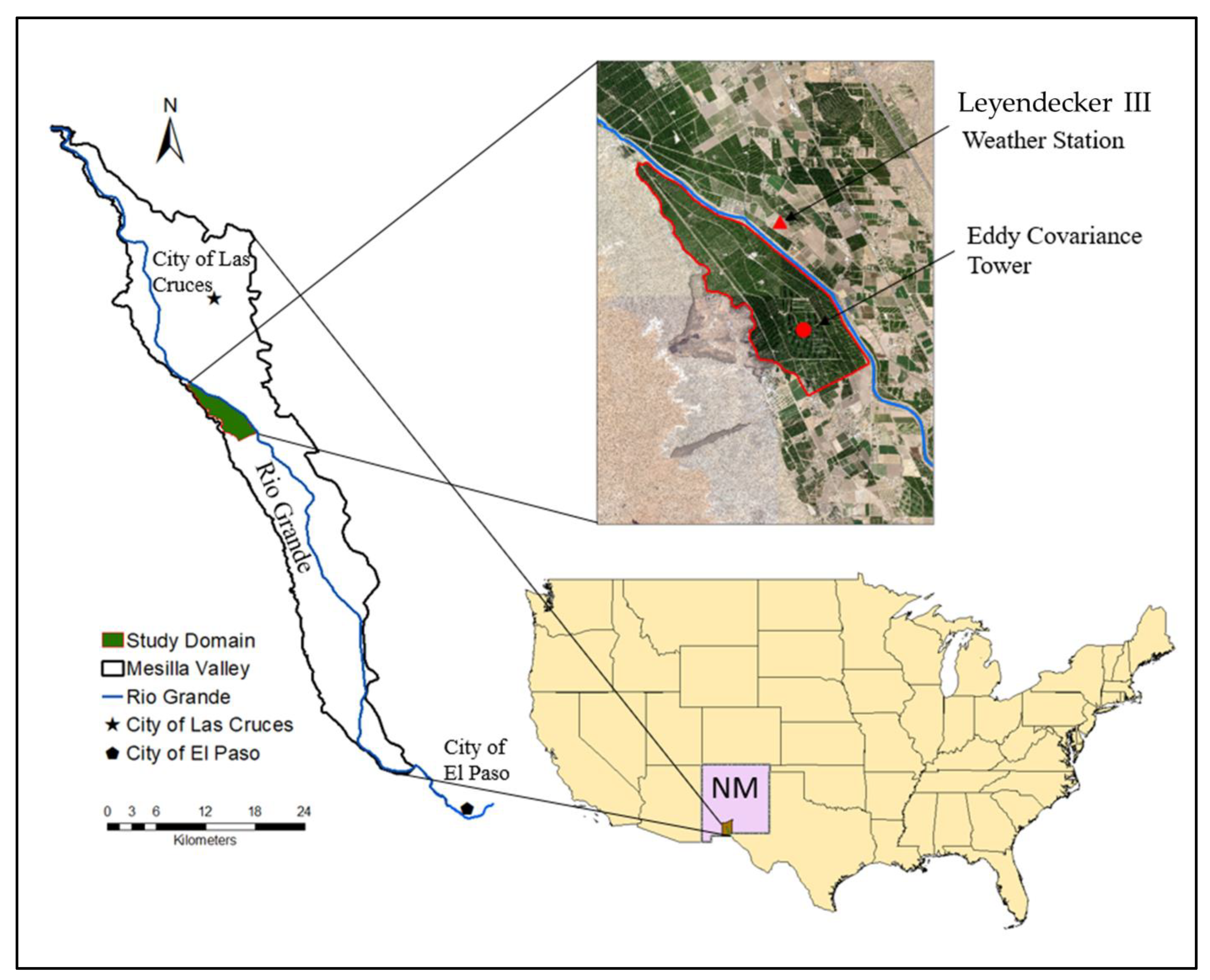
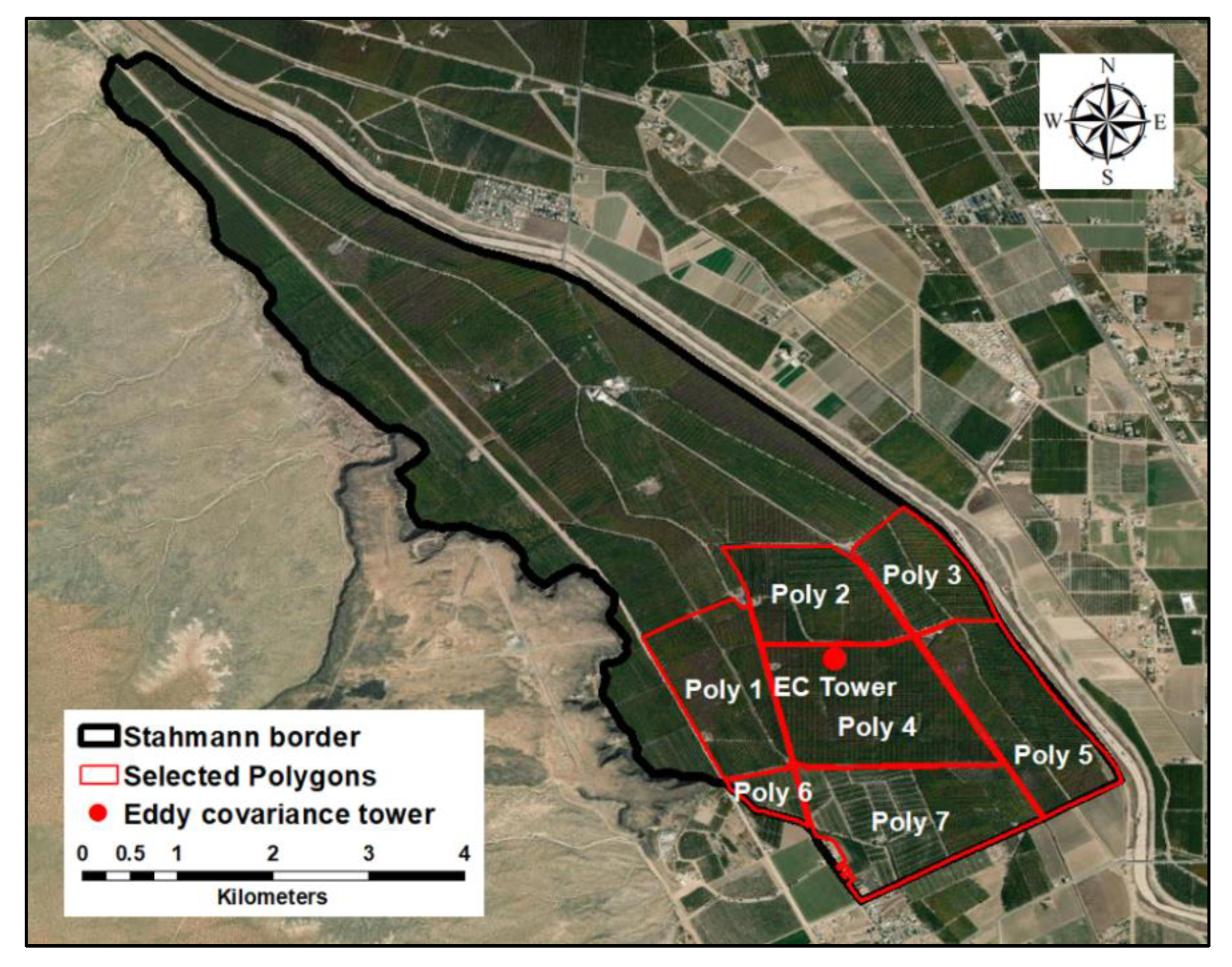
2.1. Study Site Description and Setting

The study area is located on a well-managed commercial pecan orchard owned by Stahmann Farms Incorporated in the Mesilla Valley adjacent to the Rio Grande, about 13 km south of Las Cruces, NM (Figure 1). Stahmann Farms is one of the largest pecan farms in New Mexico. It is about 1620 ha and has approximately 180,000 trees [85]. The geographic coordinate boundaries are 32°10′36.08″N and 106°44′22.39″W at 1144 m AMSL. The Rio Grande runs southward along the eastern border of the farm (Figure 1), with a naturally occurring mesa and Santo Tomas Mountain (peak elevation of about 1274 m AMSL) on the west side. Stahmann Farms Incorporated is divided into the Santo Tomas Farm and the Snow Farm. The study location is in the Santo Tomas Farm, which is about 4.8 km long and has a maximum width of about 2.4 km. The pecan trees are mainly of the “Western” (synonym “Western Schley”) cultivar [85] and mature (60 years and older). The tree spacing is 9.1 m by 9.1 m, with an average height of 16 m and trunk diameters ranging from 38 to 50 cm. The trees are mechanically pruned (hedged and topped) in alternate rows after the harvest, keeping them at an average height of about 16 m. This practice became popular among Mesilla Valley pecan farmers in the early 2000s to allow better tree canopy sunlight distribution, reduce the intensity of fluctuation in nut yields, and maximize nut quality. Eddy covariance instrumentation for measuring ET was mounted on a tower located within the southeastern fields of the farm (red circle, Figure 1). Pertinent weather data were collected from the Leyendecker III weather station (red triangle, Figure 1), located approximately 1 km away from the farm at geographical coordinates of 32°12′3.26″N and 106°44′34.00″W, with an elevation of 1176 m AMSL.

The soils of the study area, as described by Bulloch and Neher [86], are alluvial flood plains, often with a top 15 cm of clay loam and sandy soils below it extending to more than 3 m deep. The predominant soil series in the study area comprises Anapra clay loam, Agua silt loam, Glendale clay loam, and Anthony–Vinton loams. The farmland is laser-leveled and split into plots with borders for flood irrigation, an irrigation method known as “dead-level irrigation”. Farmers in the Mesilla Valley commonly use this method to irrigate mature pecan trees that have developed an expansive root system. The technique allows the grower to refill the root zone of mature trees to obtain high nut quality and yield, in addition to a proper amount of fertilizer applications. The primary source of irrigation water is the Rio Grande when available, and it is augmented with groundwater during drought years when surface water is unavailable. Surface water from the Rio Grande is distributed to farmers in the Mesilla Valley by a network of irrigation canals managed by the Elephant Butte Irrigation District (EBID). According to LaRock and Ellington [87], the orchard in this study was irrigated in the past with 12,200 to 18,300 m³ per ha of water a year (1220 to 1830 mm per year) with a typical two-week irrigation frequency during the summer months. Nut quality decreases when the trees are water-stressed during the nut-filling stage [88].

2.2. Climate

The climate of the Mesilla Valley region is semiarid. It is characterized by low and variable precipitation, large diurnal and moderate temperature ranges, low average relative humidity, and plenty of sunshine [89]. Malm’s [89] analysis of 109 years of historical data from 1892 to 2000 for Las Cruces, considered here as representing the climate of the Mesilla Valley study area, is summarized. The amount of precipitation in the region varies considerably with the changing seasons. The annual rainfall ranges from 203 to 229 mm, with a mean of 222 mm. Most rainfall (>50%) is received during the summer monsoon months of July and September. The dry season extends from November to May. The mean monthly temperatures vary from 5.5 °C in January to 26.6 °C in July, with a mean annual temperature of 15.8 °C. The mean monthly relative humidity ranges from 37% to 62% with an average of 52% in the early mornings and 16% to 34% with an average of 26% in the late afternoons. The solar radiation for the region ranges between 12 and 31 MJ/m², with an average of 22 MJ/m².

During the five years of this study, the mean monthly temperatures varied from 6.4 to 27.2 °C, with an average of 17.05 °C. June, July, and August are the warmest months. The highest temperatures are often observed in June and July and occasionally in August. In June, July, and August 2020, the air temperature exceeded 38 °C for 33 days. The highest temperature of 42.4 °C was measured on 23 June 2017, and the lowest temperature of −10.1 °C was measured on 2 January 2021. The mean monthly relative humidity varied from 38% to 56%, averaging 48.6%. The mean daily relative humidity ranged from 16% to 88%. Low humidity values were observed in the late afternoons, and high humidity in the early mornings. The annual precipitation ranged from 171 to 283 mm, averaging 226 mm. The lowest precipitation of 171 mm occurred in 2020, while the highest precipitation of 283 mm occurred in 2017. The monthly average wind speeds ranged from 1.21 to 2.15 m/s and averaged 1.56 m/s. Higher winds occur in March and April, with a maximum daily mean of 6 m/s. The mean monthly solar radiation ranged from 11 to 29 MJ/m², with an annual average of 20 MJ/m². Evapotranspiration values referenced to grass using the ASCE-standardized equation (Penman–Monteith equation) were 1586, 1547, 1500, 1518, and 1474 mm for 2017 to 2021, respectively.

2.3. Measurement of Evapotranspiration Using Eddy Covariance

Evapotranspiration of the mature pecan orchard was measured in 2004 and 2005 using the one-propellor eddy covariance (OPEC) instrumentation installed on a 23 m tall triangulated tower, 7 m above the canopy. The details of instrumentation and measurements are described in [8,85]. Measurements included flux densities of net radiation (Rn), sensible heat (H), and soil heat (G). From the measurements, latent heat flux (LE) was determined as a residual in the energy budget (LE = Rn-G-H) and converted to an equivalent depth of water (ET) by dividing LE by the latent heat of vaporization and density of water. The ET measurements for 2004 and 2005 were obtained every 30 min and summed to daily (24 h) values.

2.4. Evapotranspiration (ETec)

The daily ET values of monotypic mature pecan for 2017 to 2021, referred to here as ETec, were determined from the developed daily Kc derived from eddy covariance measurements and ETo from climate data in 2004 and 2005 by Reveles [85]. The Kc is a ratio of the crop ET when the crop is grown in large fields under optimum growing conditions [90] to the reference crop (short or tall) evapotranspiration (ASCE-EWRI) [91]. The ET_o in 2004 and 2005 were determined by the American Society of Civil Engineers Environmental and Water Resources Institute (ASCE-EWRI) method [91], similar to the FAO-56 Penman–Monteith equation using weather data collected at the Chamberino weather station located (N32°3′43.8″ and W106°40′43.8″, elevation of 1145 m AMSL) in the southern part of the Mesilla Valley [85]. Reveles [85] fitted the daily Kc values as a function of the day of the year (DOY) with fourth- and third-degree polynomial functions for 2004 (R = 0.8692, n = 318 days) and 2005 (R = 0.9113, n = 224 days), respectively, that could be used to estimate the ET of mature pecan using ET_o when actual measurements were not available. Using these developed functions, Kc for each DOY from 2004 and 2005 was averaged to determine the daily Kc of mature pecan orchards, given the relatively minor differences in the pecan’s crop coefficient over the two years. The daily ETec values of the mature pecan orchards were then calculated for 2017 to 2021 using the average daily Kc and reference ET_o calculated using the ASCE-EWRI method [91] from climate data measured at the Leyendecker III weather station (Figure 1). The daily ETec values were then summed to determine the monthly values.

2.5. Comparative Analysis Procedure

The daily ETec values for 2017 to 2021 were aggregated into monthly, seasonal, and annual data. These were compared to satellite-based ET, estimated by the six models and their ensemble on the OpenET platform. Seven polygons, numbered 1 to 7, surrounding the eddy covariance tower were delineated based on the existing subsection boundaries of the farm (red polygons in Figure 2). Respective monthly ET values generated by OpenET models for the fields within those polygons were then extracted and averaged. An average of the seven polygons’ monthly ET values for each model was compared with ETec. Various statistical measures were employed for evaluation, including the coefficient of determination (R²), root mean square error (RMSE), mean bias error (MBE), standard error of the predicted y-value for each x in a regression (SEE), mean relative difference (MRD), and probability value (p-value) for assessing statistical significance, using the following formula:

$$MBE=\frac{\sum _{i=1}^n\left(y_i{-x}_i\right)}{n}$$

(1)

$$RMSE=\sqrt{\frac{{\sum _{i=1}^n\left(y_i{-x}_i\right)}^2}{n}}$$

(2)

$$MRD=\frac{\left|y_i-x_i\right|}{x_i}\times 100$$

(3)

where n is the number of observations, x sub i is the measured value using eddy covariance, and y_i is the predicted value using models.

3. Results

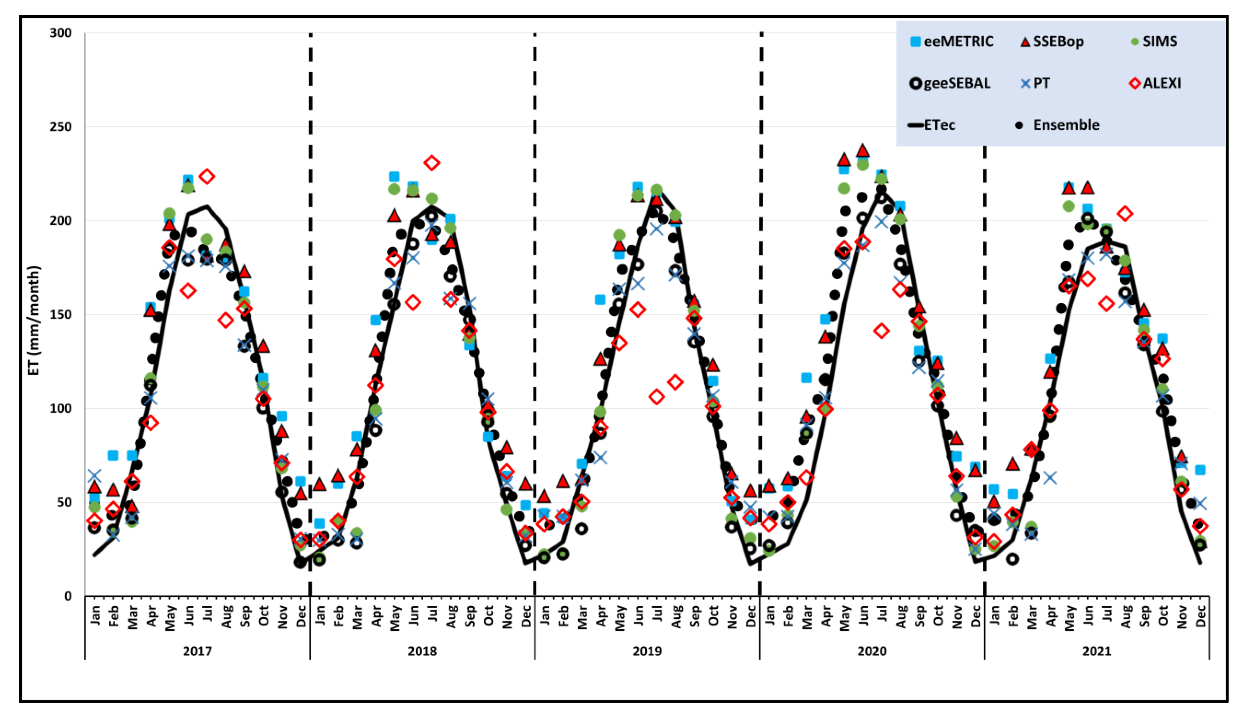
3.1. Annual and Growing Season ET of Pecan

The monthly ET for mature pecan orchards (Figure 2) in the Mesilla Valley obtained from the OpenET website (downloaded on 28 and 29 January 2022) by the six models and their ensemble was compared to the ET estimated using ETec for mature pecan orchards. OpenET remote sensing and ground-measured eddy covariance estimates for the orchard varied monthly, annually, and among the models. All the models captured the typical annual cycle of pecan ET, with low ET values during the winter months of January to March and November and December when the plants are dormant, increasing during the growing season in spring and reaching the peak in the summer months, and then declining after summer (Figure 3). The monthly ET values from 2017 to 2021 are listed in

Table A1. Growing season (GS) monthly evapotranspiration of pecan orchards estimated by eddy covariance (ETec) and by OpenET platform remote sensing-based ET models for 2017 to 2021. MRD-GS is the annual mean relative difference for the GS.

ET (mm/month) 2017
Month	ETec	geeSEBAL	eeMETRIC	SSEBop	SIMS	PT-JPL	ALEXI/DisALEXI	Ensemble
January	21.91	36.28	52.32	58.70	47.38	64.20	40.21	49.65
February	31.16	35.11	74.86	56.95	34.37	32.61	46.40	42.57
March	66.27	41.49	74.98	48.10	39.68	41.92	61.13	49.09
April	106.86	112.39	153.78	152.60	116.01	105.60	92.31	120.31
May	162.63	184.88	201.24	198.39	203.72	175.87	185.71	190.49
June	203.35	178.90	221.65	219.18	217.37	181.19	162.63	196.53
July	207.43	179.33	181.43	181.75	189.97	178.71	223.56	181.81
August	195.70	178.92	179.40	187.44	183.45	175.75	147.00	178.83
September	157.63	133.07	162.33	173.20	156.31	133.72	153.14	151.95
October	115.19	100.22	116.11	133.47	111.67	109.78	105.11	109.45
November	53.36	55.29	95.84	88.26	68.03	72.64	70.99	74.08
December	17.20	17.96	61.08	54.98	27.14	30.48	29.85	30.62
Total	1338.69	1253.83	1575.02	1553.02	1395.10	1302.48	1318.04	1375.38
GS	1148.79	1067.71	1215.94	1246.03	1178.50	1060.62	1069.46	1129.38
MRD-GS	---	7.1%	5.8%	8.5%	2.6%	7.7%	6.9%	1.7%
ET (mm/month) 2018
January	24.21	19.31	38.71	59.89	20.48	29.74	30.15	28.98
February	30.88	29.75	59.80	64.68	39.94	32.84	40.08	41.21
March	62.75	28.24	85.11	78.41	33.60	30.38	63.60	52.83
April	112.52	88.25	147.00	131.10	99.03	94.46	112.28	111.20
May	155.90	155.41	223.45	203.05	216.66	166.71	179.59	189.98
June	199.79	187.51	218.31	216.18	215.95	180.20	156.53	197.50
July	207.48	202.29	189.70	193.05	211.82	197.57	230.82	199.11
August	201.18	170.37	201.01	188.98	196.11	158.56	158.02	177.50
September	153.59	147.21	133.61	140.04	137.52	155.86	141.42	142.53
October	83.72	92.61	84.83	102.58	94.55	104.93	98.05	97.20
November	48.68	54.56	63.94	79.47	46.10	60.46	66.32	61.08
December	17.60	26.96	48.41	60.12	33.74	32.03	33.66	33.75
Total	1298.30	1202.48	1493.88	1517.53	1345.50	1243.73	1310.51	1332.89
GS	1114.18	1043.65	1197.91	1174.97	1171.65	1058.29	1076.71	1115.03
MRD-GS	---	6.3%	7.5%	5.5%	5.2%	5.0%	3.4%	0.08%
ET (mm/month) 2019
January	22.02	20.49	44.22	53.56	22.27	42.54	38.37	37.60
February	28.76	22.31	41.25	61.40	22.83	42.48	42.31	38.63
March	63.41	35.74	70.53	62.91	47.72	61.69	50.38	54.86
April	98.88	86.61	157.87	126.61	98.17	73.79	89.85	98.93
May	145.40	155.47	182.23	187.49	192.29	163.57	134.78	170.54
June	186.60	176.56	218.05	213.73	213.45	166.50	152.70	190.96
July	217.71	204.96	215.18	211.71	216.32	195.62	106.19	207.41
August	204.85	173.26	199.52	202.18	202.79	171.27	114.05	188.63
September	143.62	135.26	155.31	157.51	152.02	139.65	148.04	147.77
October	97.48	95.65	114.61	123.35	103.72	106.81	101.04	105.56
November	47.09	36.65	50.62	65.72	41.30	60.74	52.48	51.52
December	17.20	25.18	40.78	56.40	30.78	47.46	41.61	40.57
Total	1273.02	1168.13	1490.18	1522.56	1343.67	1272.13	1071.80	1332.98
GS	1094.54	1027.76	1242.78	1222.57	1178.76	1017.21	846.65	1109.80
MRD-GS	---	6.1%	13.5%	11.7%	7.7%	7.1%	22.7%	1.4%
ET (mm/month) 2020
January	22.39	27.00	57.53	59.05	24.11	42.09	38.31	41.19
February	27.87	39.15	58.58	63.09	43.09	42.39	50.01	48.52
March	51.22	86.79	116.22	95.89	86.24	91.26	63.18	89.65
April	97.60	115.30	147.34	138.54	100.19	105.71	99.56	115.07
May	155.25	182.69	227.36	232.96	217.04	177.36	185.08	204.48
June	196.16	201.26	231.93	237.82	229.73	186.79	188.74	212.89
July	215.97	212.30	224.63	223.86	222.12	199.46	141.36	216.90
August	205.07	176.72	207.77	203.48	200.78	166.97	163.36	187.30
September	152.82	125.01	130.63	154.50	143.91	121.82	146.26	137.57
October	103.39	101.42	125.50	124.32	112.13	114.76	107.06	114.21
November	56.49	42.94	74.41	84.36	52.99	56.46	63.86	61.29
December	18.31	34.87	68.83	67.32	25.08	25.07	31.39	33.25
Total	1302.54	1345.45	1670.74	1685.18	1457.41	1330.15	1278.17	1462.32
GS	1126.26	1114.70	1295.16	1315.47	1225.90	1072.88	1031.42	1188.42
MRD-GS	---	1.0%	15.0%	16.8%	8.9%	4.7%	8.4%	5.5%
ET (mm/month) 2021
January	21.40	40.79	56.99	50.59	26.69	44.00	29.07	40.47
February	29.94	19.64	54.31	70.84	39.44	38.28	43.36	41.91
March	62.72	33.49	77.29	78.80	36.92	33.12	78.07	55.85
April	103.02	95.78	126.50	119.85	95.47	63.05	98.89	101.04
May	152.16	167.19	217.66	217.71	207.67	168.43	165.25	189.16
June	185.10	201.20	206.44	217.80	198.10	180.03	168.99	201.57
July	188.89	193.96	195.66	186.35	195.29	182.10	155.88	189.74
August	186.09	161.41	172.48	174.93	178.61	156.98	203.77	168.71
September	139.43	133.82	145.43	152.64	141.74	135.30	136.80	138.95
October	100.95	98.38	137.16	132.20	110.12	106.86	126.35	118.03
November	45.21	56.79	71.14	74.70	60.86	70.80	56.85	64.87
December	17.89	27.17	67.10	29.48	29.27	49.40	37.35	35.39
Total	1232.81	1229.64	1528.15	1505.89	1320.17	1228.34	1300.62	1345.69
GS	1055.64	1051.75	1201.33	1201.48	1126.99	992.74	1055.92	1107.20
MRD-GS	---	0.37%	13.8%	13.8%	6.7%	6.0%	0.03%	4.9%
Total ET (2017–2021)
Annual Avg.	1289	1240	1552	1557	1372	1275	1256	1370
MRD-Annual	---	4.4%	23.7%	24.2%	7.5%	1.2%	3.0%	7.3%
GS Avg.	1108	1061	1231	1232	1176	1040	1016	1130
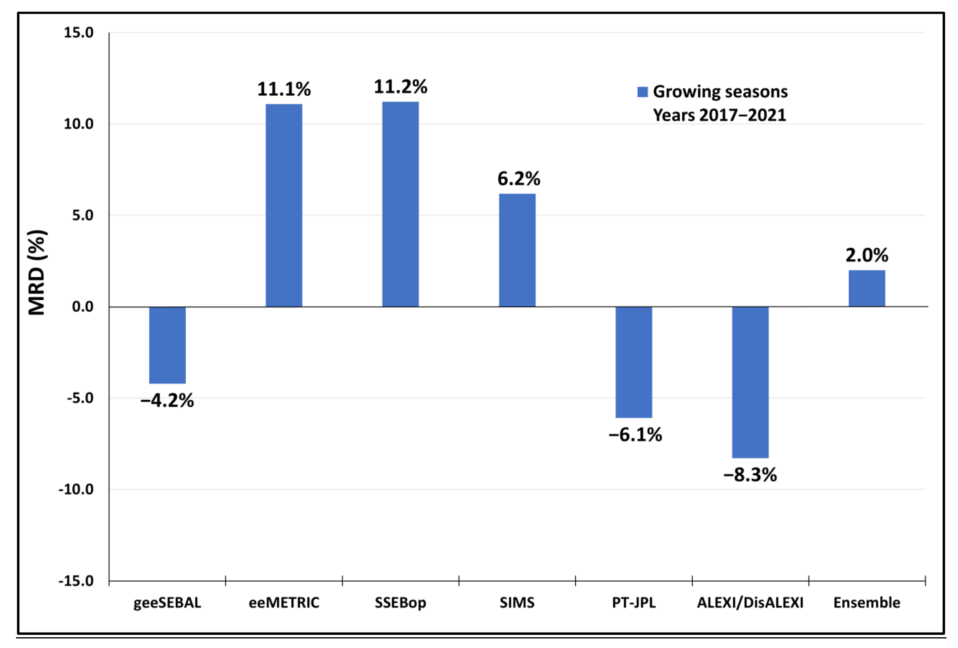
MRD-GS	---	4.2%	11.1%	11.2%	6.2%	6.1%	8.3%	2.0%

(Appendix A), and the time series is shown in Figure 3. The mean annual ET for all the models during the five years varied from 1240 mm (Std. Dev. ± 67.1 mm) estimated by geeSEBAL to 1557 mm (Std. Dev. ± 73.8 mm) estimated by the SSEBop model. The mean annual ET estimated by eddy covariance was 1289 mm. All models’ growing season ET values fell within the range of 1016–1232 mm, as previously reported by Samani et al. [8], Sammis et al. [6], and Miyamoto [7].

During the growing season, i.e., April to October, the mean annual ET varied from 1016 mm (Std. Dev. ± 37.11 mm) using the ALEXI/DisALEXI model to 1232 mm using SSEBop (Std. Dev. of ±38.09 mm). The mean annual ET estimated by eddy covariance was 1108 mm (Std. dev. ± 42.35 mm). A comparison of each model’s ET with ETec using linear regression is explained in the following sections.

3.2. geeSEBAL

The geeSEBAL ET estimates ranged from 1168 to 1345 mm per year with a 5-year average of 1240 mm and from 1028 to 1115 mm with a 5-year average of 1061 mm during the growing season. Comparing the 5-year average ETec of 1289 mm and the growing season ET of 1108 mm, the absolute MRD was 4.4% and 4.2%, respectively. A comparison of the geeSEBAL model and ETec on an annual basis for 2017 to 2021 (

Table A2. Comparison of statistical criteria between the OpenET models-based estimated ET and the ground-based ETec (mm/mo) of pecan orchards for each year (N = 12) from 2017 to 2021.

Year 2017
Model/Criteria	Intercept	Slope	R2	RMSE	MBE	SEE	p−Value
geeSEBAL	6.50	0.88	0.9494	18.1	−7.2	15.6	<0.05
eeMETRIC	45.4	0.77	0.8991	31.1	19.7	19.7	<0.05
SSEBop	36.0	0.84	0.8998	28.8	17.9	21.4	<0.05
SIMS	9.60	0.96	0.9344	18.5	4.7	19.3	<0.05
PT-JPT	20.1	0.79	0.9288	21.3	−3.0	16.8	<0.05
ALEXI/DisALEXI	17.7	0.83	0.9000	22.8	−1.7	21.0	<0.05
Ensemble	19.4	0.85	0.9454	17.8	3.1	15.7	<0.05
Year 2018
geeSEBAL	−0.11	0.93	0.9601	16.9	−8.2	15.4	<0.05
eeMETRIC	27.0	0.90	0.8919	28.2	16.3	24.0	<0.05
SSEBop	40.0	0.80	0.9312	27.6	18.3	16.6	<0.05
SIMS	−1.40	1.05	0.9224	21.9	3.9	23.3	<0.05
PT-JPT	10.0	0.87	0.9298	19.3	−4.6	18.2	<0.05
ALEXI/DisALEXI	17.9	0.84	0.9040	22.1	1.0	21.1	<0.05
Ensemble	12.8	0.91	0.9575	15.10	2.90	14.7	<0.05
Year 2019
geeSEBAL	−2.40	0.94	0.9726	15.1	−9.1	12.5	<0.05
eeMETRIC	22.5	0.96	0.9379	25.1	18.1	18.8	<0.05
SSEBop	33.1	0.88	0.9546	26.0	20.8	14.7	<0.05
SIMS	−1.70	1.10	0.9594	17.2	5.9	16.8	<0.05
PT-JPT	23.6	0.78	0.9483	20.0	−0.08	13.8	<0.05
ALEXI/DisALEXI	35.7	0.51	0.7214	44.1	−16.8	24.0	<0.05
Ensemble	14.8	0.91	0.9738	13.2	5.0	11.3	<0.05
Year 2020
geeSEBAL	16.0	0.89	0.9297	19.1	3.6	18.7	<0.05
eeMETRIC	46.0	0.86	0.8688	40.1	30.7	26.0	<0.05
SSEBop	44.3	0.89	0.9101	38.4	31.9	21.7	<0.05
SIMS	9.70	1.03	0.9330	23.6	12.9	21.5	<0.05
PT-JPT	24.6	0.79	0.9262	21.8	2.3	17.5	<0.05
ALEXI/DisALEXI	28.3	0.72	0.8727	28.0	−2.0	21.4	<0.05
Ensemble	23.8	0.90	0.9345	22.7	13.3	18.7	<0.05
Year 2021
geeSEBAL	1.60	0.98	0.9450	15.2	−0.26	16.9	<0.05
eeMETRIC	37.9	0.87	0.9037	31.7	24.6	19.9	<0.05
SSEBop	30.0	0.93	0.9085	30.0	22.8	20.6	<0.05
SIMS	3.40	1.04	0.9304	20.6	7.30	19.9	<0.05
PT-JPT	16.80	0.83	0.8815	22.3	−0.37	21.3	<0.05
ALEXI/DisALEXI	19.80	0.86	0.9435	17.1	5.60	14.8	<0.05
Ensemble	15.70	0.94	0.9507	17.0	9.40	14.9	<0.05

in Appendix A) using a linear regression showed a strong positive relationship, with an R² ranging from 0.9297 to 0.9726 (N = 12 months). The geeSEBAL estimates had the smallest RMSE and SEE values, ranging 15–19 and 12–19 mm/mo, respectively, compared to all other OpenET model comparisons with ETec. The geeSEBAL slightly underestimated ET when compared to ETec for 2017 (MBE = −7.2 mm/mo), 2018 (MBE = −8.2 mm/mo), 2019 (MBE = −9.1 mm/mo), and 2021 (MBE = −0.26 mm/mo) and overestimated ET in 2020 (3.6 mm/mo).

During the five years (N = 60 months; 12 months × 5 years), the geeSEBAL-estimated ET correlated with the ETec with an R² of 0.9449, a small RMSE of 17 mm/mo, and a SEE of 16 mm/mo. During the growing season, when the plants are actively growing, from 2017 to 2021 (N = 35; 7 months × 5 years; p < 0.05), the geeSEBAL model had the highest agreement with the ETec among all OpenET models with R², RMSE, and SEE of 0.8504, 17 mm/mo, and 15 mm/mo, respectively (p-value < 0.5). See

Table A3. Comparison between the OpenET models with ETec (mm/mo) for annual (N = 60 months) and growing seasons (N = 35 months) during the entire 2017 to 2021 period.

Model/Criteria	Number Observations, N (Months)	Intercept	Slope	R2	RMSE	MBE	SEE	p−Value
geeSEBAL	60	4.50	0.92	0.9449	17	−4.2	16	<0.05
	35	13.32	0.87	0.8564	17	−7	15	<0.05
eeMETRIC	60	35.73	0.87	0.8906	32	22	21	<0.05
	35	58.32	0.74	0.6249	32	18	25	<0.05
SSEBop	60	36.82	0.86	0.9122	30	22	19	<0.05
	35	57.15	0.75	0.6974	29	18	21	<0.05
SIMS	60	3.89	1.03	0.9331	20	7	19	<0.05
	35	10.82	0.99	0.7970	23	10	22	<0.05
PT-JPT	60	19.01	0.81	0.9203	21	−1.1	17	<0.05
	35	23.62	0.79	0.8068	21	−10	17	<0.05
ALEXI/DisALEX	60	24.31	0.75	0.8430	28	−3	23	<0.05
	35	53.53	0.58	0.4365	35	−13	28	<0.05
Ensemble	60	17.43	0.90	0.9477	17	7	15	<0.05
	35	29.37	0.83	0.8234	18	3	17	<0.05

in Appendix A.

3.3. eeMETRIC

The eeMETRIC ET estimates ranged from 1490 to 1671 mm per year with a 5-year average of 1552 mm and from 1198 to 1295 mm with a 5-year average of 1231 mm during the growing season. Comparing the 5-year average ETec of 1289 mm and the growing season ET of 1108 mm, the absolute MRD was 23.7% and 11.1%, respectively (Figure 4). A comparison of the eeMETRIC model and ETec on an annual basis for 2017 to 2021 (Table A2) using a linear regression showed a positive relationship, with an R² ranging from 0.8688 to 0.9379 (N = 12 months). When compared with ETec, the eeMETRIC-estimated RMSE and SEE had a range of 25–40 and 18–26 mm/mo. The eeMETRIC overestimated ET when compared to ETec for 2017 (MBE = 19.7 mm/mo), 2018 (MBE = 16.3 mm/mo), 2019 (MBE = 18.1 mm/mo), 2020 (30.7 mm/mo), and 2021 (MBE = 24.6 mm/mo).

During the five years (N = 60 months; 12 months × 5 years), the eeMETRIC-estimated ET correlated with the ETec with an R² of 0.8906, an RMSE of 32 mm/mo, and a SEE of 21 mm/mo. During the growing season, when the plants are actively growing, from 2017 to 2021 (N = 35; 7 months × 5 years; p < 0.05), eeMETRIC model comparison with the ETec resulted in an R² of 0.6249, an RMSE of 32 mm/mo, and a SEE of 25 mm/mo (p-value < 0.5). See Table A3.

The estimated ET values of eeMETRIC were consistently higher during the non-growing season, resulting in a higher annual ET than those of ETec. These high estimates are also shown in Figure 3, with a slight shift in the ET patterns. This occurred during the early half of the growing season for the five years. De Oliveira et al. [92] stated that the high moisture content from irrigation events accounts for the uncertainties associated with estimating ET during the non-growing season by the METRIC model. A high residual water supply from irrigation influences the advection effect, resulting in a low estimate of sensible heat and an overestimation of ET. A previous study by Singh and Irmak [66] compared the METRIC-based estimate of ET with the ETec in central Nebraska, USA. Their results demonstrated the uncertainty of the METRIC model in estimating sensible heat for high residual soil moisture content, with a high RMSE of 122 W m⁻² for sensible heat. Higher ET estimates compared to ETec by METRIC were also observed by Wagle et al. [93] for sorghum crops during the 2012 and 2013 growing seasons. They reported that the METRIC model overestimated the growing season ET for sorghum by approximately 25–30%.

3.4. SSEBop

The SSEBop ET estimates ranged from 1506 to 1685 mm per year with a 5-year average of 1557 mm and from 1175 to 1315 mm with a 5-year average of 1232 mm during the growing season. Comparing the 5-year average ETec of 1289 mm and the growing season ET of 1108 mm, the absolute MRD was 24.2% and 11.2%, respectively (Figure 4). A comparison of the SSEBop ET model and ETec on an annual basis for 2017 to 2021 (Table A2) using a linear regression showed a positive relationship, with an R² ranging from 0.8991 to 0.9546 (N = 12 months). More than 89.9% of variations in the estimated ET by the SSEBop model can be explained by the ETec annually for five years. During this time frame, SSEBop’s RMSE varied between 26 and 38 mm/mo, and SEE ranged from 14 to 22 mm/mo. For each year from 2017 to 2021, similar to eeMETRIC, the SSEBop also overestimated ET when compared to ETec (MBE = 17.9, 18.3, 20.8, 31.9, and 22.8 mm/mo; Table A2).

During the five years (N = 60 months; 12 months × 5 years), the SSEBop-estimated ET correlated with the ETec with an R² of 0.9122, an RMSE of 30 mm/mo, and a SEE of 19 mm/mo (Table A3). During the growing season, when the plants are actively growing, from 2017 to 2021 (N = 35; 7 months × 5 years), the SSEBop model comparison with the ETec resulted in R², RMSE, and SEE of 0.6974, 29 mm/mo, and 21 mm/mo, respectively (p-value < 0.5). Like eeMETRIC, the SSEBop also exhibited a slight shift in the annual ET pattern (Figure 3), estimating higher ET values during the earlier part of the growing season. Despite the similarity in ET estimates for pecan on a monthly, annual, and average basis for five years, the SSEBop model outperformed the eeMETRIC model based on the statistical measures employed. During the growing seasons from 2017 to 2021 (N = 35 months), the SSEBop model demonstrated better agreement with the ETec. See Table A2 and Table A3. However, both model estimates of ET were statistically significant (p < 0.05) compared to the ETec. Other studies, such as those by Chen et al. [46], have shown that SSEBop model ET estimates of different land cover types (cropland, grassland, forest, shrubland, and woody savanna) using MODIS satellite data agreed well (R² = 0.86) with eddy covariance-measured ET. For the pecan orchard in this study, 69.7% (R² = 0.6974, N = 35) of the variance in ET estimates by SSEBop can be explained by the ETec during the growing season.

3.5. SIMS

The SIMS ET estimates ranged from 1320 to 1457 mm per year with a 5-year average of 1372 mm and from 1127 to 1226 mm with a 5-year average of 1176 mm during the growing season (Table A1). Comparing the 5-year average ETec of 1289 mm and the growing season ET of 1108 mm, the absolute MRD was 7.5% and 6.2%, respectively. SIMS’s ET estimates were in good agreement with the ETec from 2017 to 2021 (Table A1 and Table A2). Over 92% of the proportion of variance in ET estimated by SIMS can be explained by the ETec. A comparison of SIM’s ET estimates with ETec using linear regression analysis during the five years on an annual and growing season basis is presented in Table A3. Similar to geeSEBAL, on average, for the five years, the SIMS model ET estimates also agreed well with the ETec (R² = 0.9331, RMSE of 20 mm/mo, and SEE of 19 mm/mo; N = 60 months). During the growing season (N = 35 months), the RMSE of 23 mm/mo and SEE of 22 mm/mo were slightly higher than the geeSEBAL. The SIMS model ET estimates and ETec were statistically significant (p < 0.05). However, minor variances were observed between SIMS and ETec in May, June, and July as the plants approached peak growth, as shown in Figure 3. The SIMS model estimated slightly higher ET values than the ETec during those months.

3.6. PT-JPL

The PT-JPL-estimated ET ranged from 1228 to 1330 mm per year with a 5-year average of 1275 mm and from 993 to 1073 mm with a 5-year average of 1040 mm during the growing season (Table A1). Comparing the 5-year average ETec of 1289 mm and the growing season ET of 1108 mm, the absolute MRD was 1.2% and 6.1%, respectively (Table A2). The PT-JPL underestimated ET by −6.1% compared to ETec (Figure 4). A comparison of PT-JPL model ET estimates and ETec using linear regression for each year (Table A2) and for the five years (N = 60 months) and growing season (N = 35 months) is presented in Table A3. The R² ranged from 0.8815 to 0.9483, and the RMSE ranged from 19 to 21 mm/mo (N = 12 months). For the five years, the values were R² of 0.9203, RMSE of 21 mm/mo, and SEE of 17 mm/mo (N = 60 months), while R² of 0.8068, RMSE of 21 mm/mo, and SEE of 17 mm/mo were recorded during the growing season (N = 35 months). The comparison of the ET estimates by PT-JPL with the ETec was correlated and statistically significant at p < 0.05. The MBEs for 2017 to 2021 were −3.0, −4.6, −0.08, 2.3, and −0.37 mm/mo, respectively. The PT-JPL average annual ET for five years was close to the ETec (1275 vs. 1289 mm) with an MRD of 1.2%. The PT-JPL ET followed the same trend as the ETec during the five years (Figure 3), with some deviation in May, June, and July. The PT-JPL values were slightly higher during the three months than the ETec (Table A1).

3.7. ALEXI/DisALEXI

The ALEXI/DisALEXI ET estimates ranged from 1072 to 1318 mm per year with a 5-year average of 1256 mm and from 847 to 1077 mm with an average of 1016 mm during the growing season. The ETec estimates for the 5-year annual average and growing season averages were 1289 and 1108 mm. The absolute MRD of ALEXI/DisALEXI ET compared to the ETec for a yearly average was 2.6%, and the growing season average was 8.3% for the five years, overestimating ET by just a small percentage (Table A1). However, on an annual basis and using regression analysis for comparison with the ETec, the R² in 2019 was very low (R² = 0.7214), and the RMSE was high at 44 mm/mo compared to other OpenET model estimates. The ALEXI/DisALEX ET estimates were not consistent annually compared to ETec. On an annual basis, the model either overestimated or underestimated ET. The MBEs for 2017 to 2021 were −1.7, 1.0, −16.8, −2.0, and 5.6, respectively. For the five years (Table A3), the ALEXI/DisALEXI model ET estimates did not compare well with the ETec, especially during the peak of the growing season (R² = 0.4365, RMSE of 35 mm/mo, and SEE of 28 mm/mo, N = 35 months). A large discrepancy in ALEXI/DisALEXI model ET estimates compared to other models was observed from May to August (refer to Figure 3).

3.8. Ensemble

The ensemble model with ET estimates of mature pecan orchards showed the strongest agreement with the ETec estimates. See Table A1, Table A2 and Table A3. The ensemble ET estimates ranged from 1333 to 1462 mm per year, with a 5-year average ET of 1370 mm. During the growing season, the ensemble ET ranged from 1107 to 1188 mm, with a 5-year average of 1130 mm. Comparing the 5-year average annual ETec of 1289 mm and the average growing season ET of 1108 mm, the absolute MRD was 7.3% and 2.0% (Figure 4), respectively. A comparison of the ensemble ET estimates to ETec resulted in R² > 0.93 for all the years from 2017 to 2021, ranging from 0.9345 to 0.9738 (R² = 0.9477 for N = 60 months; R² = 0.8234 for N = 35 months). The RMSE ranged from 13 to 23 mm/mo, and the SEE ranged from 11 to 19 mm/mo for these years for the same period (refer to Table A1, Table A2 and Table A3 in Appendix A).

4. Discussion

The average ET estimates during the growing season for the five years (N = 35 months) when the plants are active varied among the models, especially during the early and middle growth stages of pecan from April to July (Figure 3). Overall, all ET estimates of pecan orchards by the models on the OpenET platform were linearly related to the ETec estimates (Table A3) with R² > 0.84 (N = 60 months) during the five years and were statistically significant (p < 0.05). Monthly aggregated ET estimates during the five years (N = 60 months) by the ensemble model were overestimated in the winter months (January, February, November, and December) and also during the early part of the growing season in May and June and underestimated in July, August, and September during the peak of the growing season when compared to the ETec. The geeSEBAL estimates were closer to the ETec estimates in the winter months but underestimated ET during March, June, July, August, and September. The eeMETRIC and SSEBop monthly aggregated ET estimates followed the same trend during the year. Compared with ETec, the MRD for the two models’ average annual ET for the five years was about 24% and 11% (Figure 4) during the growing season. The two models overestimated ET compared to ETec and geeSEBAL for most months, with a higher discrepancy during the first half of the year (January–June). The SIMS monthly ET estimates generally had a strong agreement with the ETec (MRD = 6.2%, N = 35) but overestimated ET in May and June. The PT-JPL ET estimates varied during the year, with higher values in wintertime and lower values during the summer months of June to September (MRD = −6.1% during the growing season). The ALEXI/DisALEXI ET estimates varied interannually compared to the other models’ ET estimates. High variability was noticed during May, July, and August, with lower mean monthly ETs than ETec. The ET estimates during winter when the plants are dormant are expected to have high uncertainty due to many factors, not only eddy covariance measurements and energy imbalances involved with ground measurements [94,95] but also remote sensing-based models [96,97].

Similar studies to assess OpenET models with eddy covariance measurements for various crops have been conducted, for example, by Melton et al. [84] and Volk et al. [98]. They concluded that overall, the crop ET estimated by the ensemble model correlated well with the ETec ground measurements every month (R² > 0.85 and RMSE < 30 mm/month). This study also shows that the ensemble modeling on the OpenET platform estimates ETec the best, especially during the growing season when managing irrigation water to grow crops is most critical in a region where water is scarce. The assessment of the OpenET platform in this study focused on the monthly and seasonal ET of mature pecan orchards. However, further assessment of OpenET is needed for estimating the ET of young pecan orchards with exposed soil or grasses between the trees, different irrigation systems, and where cropping patterns are varied. While the remote sensing-based OpenET has its limitations of not providing daily ET values, it does provide valuable information that could be used as a tool for planning sustainable water use, identifying areas in the field that need attention due to salinity, nutrient deficiencies, plant disease, or water clogging.

5. Conclusions

Six remote sensing-based ET models (geeSEBAL, eeMETRIC, SSEBop, SIMS, PT-JPL, ALEXI/DisALEXI) and their ensemble were evaluated on the OpenET platform by comparing their monthly ET estimates with eddy covariance estimates from 2017 to 2021. The models were assessed for estimating the monthly, growing season, and annual ET of a mature pecan orchard at the field scale in the Mesilla Valley, NM, from 2017 to 2021. The average ET estimates during the growing season for the five years (N = 35 months) when the plants are active varied among the models, especially during the early and middle growth stages of pecan from April to July. Overall, all ET estimates of pecan orchards by the models were linearly related to the ETec estimates with R² greater than 0.84 (N = 60 months) during the five years and were statistically significant (p < 0.05). The ensemble approach, which takes into account all the models and minimizes the biases among the models, showed the best results compared with ground-measured ETec estimates, especially during the growing season (absolute MRD = 2%), when the management of irrigation water to grow crops such as pecan is most critical in regions where water is scarce. However, assessment of OpenET is still needed for young pecan orchards with exposed soil or grasses between them and where cropping patterns are varied.

References

- U.S. Department of Agriculture–National Agricultural Statistics Service (NASS) New Mexico Field Office. 2018; Agricultural Statistics. Available online: https://www.nass.usda.gov/Statistics_by_State/New_Mexico/Publications/Annual_Statistical_Bulletin/2018/2018-NM-Ag-Statistics.pdf (accessed on 22 November 2022).
- U.S. Department of Agriculture–National Agricultural Statistics Service (NASS) New Mexico Field Office. 2020; Agricultural Statistics. Available online: https://www.nass.usda.gov/Statistics_by_State/New_Mexico/Publications/Annual_Statistical_Bulletin/2020/2020-NM-Ag-Statistics.pdf (accessed on 22 November 2022).
- U.S. Department of Agriculture–National Agricultural Statistics Service (NASS). 2017; Agricultural Statistics. Available online: https://www.nass.usda.gov/Statistics_by_State/New_Mexico/Publications/Annual_Statistical_Bulletin/2017/2017-NM-AG-Statistics.pdf (accessed on 22 November 2022).
- U.S. Department of Agriculture–National Agricultural Statistics Service (NASS) New Mexico Field Office. 2019; Agricultural Statistics. Available online: https://www.nass.usda.gov/Statistics_by_State/New_Mexico/Publications/Annual_Statistical_Bulletin/2019/2019-NM-Ag-Statistics.pdf (accessed on 22 November 2022).
- U.S. Department of Agriculture–National Agricultural Statistics Service (NASS)-Crop Data Layer-CropScape. 2021. Available online: https://nassgeodata.gmu.edu/CropScape/ (accessed on 29 November 2022).
- Sammis, T.W.; Mexal, J.G.; Miller, D. Evapotranspiration of Flood-Irrigated Pecans. Agric. Water Manag. 2004, 69, 179–190. [Google Scholar] [CrossRef]
- Miyamoto, S. Consumptive water use of irrigated pecans. J. Am. Soc. Hortic. Sci. 1983, 108, 676–681. [Google Scholar] [CrossRef]
- Samani, Z.; Bawazir, A.S.; Bleiweiss, M.; Skaggs, R.; Longworth, J.; Tran, V.D.; Pinon, A. Using remote sensing to evaluate the spatial variability of evapotranspiration and crop coefficient in the lower Rio Grande Valley, New Mexico. Irrig. Sci. 2009, 28, 93–100. [Google Scholar] [CrossRef]
- Kallestad, J.C.; Sammis, T.W.; Mexal, J.G.; White, J. Monitoring and Management of Pecan Orchard Irrigation: A Case Study. Horttechnology-Alex. Va- 2006, 16, 667–673. [Google Scholar] [CrossRef]
- Senay, G.B.; Bohms, S.; Singh, R.K.; Gowda, P.H.; Velpuri, N.M.; Alemu, H.; Verdin, J.P. Operational Evapotranspiration Mapping Using Remote Sensing and Weather Datasets: A New Parameterization for the SSEB Approach. J. Am. Water Resour. Assoc. 2013, 49, 577–591. [Google Scholar] [CrossRef]
- Wagle, P.; Skaggs, T.H.; Gowda, P.H.; Northup, B.K.; Neel, J.P.S. Flux Variance Similarity-Based Partitioning of Evapotranspiration over a Rainfed Alfalfa Field Using High Frequency Eddy Covariance Data. Agric. For. Meteorol. 2020, 285–286, 107907. [Google Scholar] [CrossRef]
- French, A.; Hunsaker, D.; Bounoua, L.; Karnieli, A.; Luckett, W.; Strand, R. Remote Sensing of Evapotranspiration over the Central Arizona Irrigation and Drainage District, USA. Agronomy 2018, 8, 278. [Google Scholar] [CrossRef]
- Bawazir, A.S.; Luthy, R.; King, J.P.; Tanzy, B.F.; Solis, J. Assessment of the Crop Coefficient for Saltgrass under Native Riparian Field Conditions in the Desert Southwest: Crop coefficient of saltgrass under native field conditions. Hydrol. Process. 2014, 28, 6163–6171. [Google Scholar] [CrossRef]
- Allen, R.G.; Tasumi, M.; Morse, A.; Trezza, R.; Wright, J.L.; Bastiaanssen, W.; Kramber, W.; Lorite, I.; Robison, C.W. Satellite-Based Energy Balance for Mapping Evapotranspiration with Internalized Calibration (METRIC)—Applications. J. Irrig. Drain. Eng. 2007, 133, 395–406. [Google Scholar] [CrossRef]
- Allen, R.G.; Tasumi, M.; Trezza, R. Satellite-Based Energy Balance for Mapping Evapotranspiration with Internalized Calibration (METRIC)—Model. J. Irrig. Drain. Eng. 2007, 133, 380–394. [Google Scholar] [CrossRef]
- Bastiaanssen, W.G.M.; Menenti, M.; Feddes, R.A.; Holtslag, A.A.M. A Remote Sensing Surface Energy Balance Algorithm for Land (SEBAL). 1. Formulation. J. Hydrol. 1998, 212–213, 198–212. [Google Scholar] [CrossRef]
- Bastiaanssen, W.G.; Pelgrum, H.; Wang, J.; Ma, Y.; Moreno, J.; Roerink, G.; Van der Wal, T. A Remote Sensing Surface Energy Balance Algorithm for Land (SEBAL).: Part 2: Validation. J. Hydrol. 1998, 212, 213–229. [Google Scholar] [CrossRef]
- Bastiaanssen, W.G.M. SEBAL-based sensible and latent heat fluxes in the irrigated Gediz Basin, Turkey. J. Hydrol. 2000, 229, 87–100. [Google Scholar] [CrossRef]
- Roerink, G.J.; Su, Z.; Menenti, M. S-SEBI: A Simple Remote Sensing Algorithm to Estimate the Surface Energy Balance. Phys. Chem. Earth Part B 2000, 25, 147–157. [Google Scholar] [CrossRef]
- Su, Z. The Surface Energy Balance System (SEBS) for Estimation of Turbulent Heat Fluxes. Hydrol. Earth Syst. Sci. 2002, 6, 85–100. [Google Scholar] [CrossRef]
- Norman, J.M.; Kustas, W.P.; Humes, K.S. Source Approach for Estimating Soil and Vegetation Energy Fluxes in Observations of Directional Radiometric Surface Temperature. Agric. For. Meteorol. 1995, 77, 263–293. [Google Scholar] [CrossRef]
- Anderson, M.C.; Norman, J.M.; Mecikalski, J.R.; Otkin, J.A.; Kustas, W.P. A Climatological Study of Evapotranspiration and Moisture Stress across the Continental United States Based on Thermal Remote Sensing: 1. Model Formulation. J. Geophys. Res. 2007, 112, 2006JD007506. [Google Scholar] [CrossRef]
- Anderson, M.; Gao, F.; Knipper, K.; Hain, C.; Dulaney, W.; Baldocchi, D.; Eichelmann, E.; Hemes, K.; Yang, Y.; Medellin-Azuara, J.; et al. Field-Scale Assessment of Land and Water Use Change over the California Delta Using Remote Sensing. Remote Sens. 2018, 10, 889. [Google Scholar] [CrossRef]
- Laipelt, L.; Ruhoff, A.L.; Fleischmann, A.S.; Kayser, R.H.B.; Kich, E.D.M.; Da Rocha, H.R.; Neale, C.M.U. Assessment of an Automated Calibration of the SEBAL Algorithm to Estimate Dry-Season Surface-Energy Partitioning in a Forest–Savanna Transition in Brazil. Remote Sens. 2020, 12, 1108. [Google Scholar] [CrossRef]
- Senay, G.B. Satellite Psychrometric Formulation of the Operational Simplified Surface Energy Balance (SSEBop) Model for Quantifying and Mapping Evapotranspiration. Appl. Eng. Agric. 2018, 34, 555–566. [Google Scholar] [CrossRef]
- Melton, F.S.; Johnson, L.F.; Lund, C.P.; Pierce, L.L.; Michaelis, A.R.; Hiatt, S.H.; Guzman, A.; Adhikari, D.D.; Purdy, A.J.; Rosevelt, C.; et al. Satellite Irrigation Management Support with the Terrestrial Observation and Prediction System: A Framework for Integration of Satellite and Surface Observations to Support Improvements in Agricultural Water Resource Management. IEEE J. Sel. Top. Appl. Earth Obs. Remote Sens. 2012, 5, 1709–1721. [Google Scholar] [CrossRef]
- Pereira, L.; Paredes, P.; Melton, F.; Johnson, L.; Wang, T.; López-Urrea, R.; Cancela, J.; Allen, R. Prediction of Crop Coefficients from Fraction of Ground Cover and Height. Background and Validation Using Ground and Remote Sensing Data. Agric. Water Manag. 2020, 241, 106197. [Google Scholar] [CrossRef]
- Fisher, J.B.; Tu, K.P.; Baldocchi, D.D. Global Estimates of the Land–Atmosphere Water Flux Based on Monthly AVHRR and ISLSCP-II Data, Validated at 16 FLUXNET Sites. Remote Sens. Environ. 2008, 112, 901–919. [Google Scholar] [CrossRef]
- Hart, Q.J.; Brugnach, M.; Temesgen, B.; Rueda, C.; Ustin, S.L.; Frame, K. Daily Reference Evapotranspiration for California Using Satellite Imagery and Weather Station Measurement Interpolation. Civ. Eng. Environ. Syst. 2009, 26, 19–33. [Google Scholar] [CrossRef]
- Bastiaanssen, W.G.M. Regionalization of Surface Flux Densities and Moisture Indicators in Composite Terrain: A Remote Sensing Approach under Clear Skies in Mediterranean Climates; Wageningen University and Research: Wageningen, The Netherlands, 1995. [Google Scholar]
- Trezza, R. Evapotranspiration Using a Satellite-Based Surface Energy Balance with Standardized Ground Control; Utah State University: Cash, UT, USA, 2002. [Google Scholar]
- Tasumi, M.; Trezza, R.; Allen, R.G.; Wright, J.L. Operational Aspects of Satellite-Based Energy Balance Models for Irrigated Crops in the Semi-Arid US. Irrig. Drain. Syst. 2005, 19, 355–376. [Google Scholar] [CrossRef]
- Bezerra, B.G.; Silva, B.B.D.; Santos, C.A.C.D.; Bezerra, J.R.C. Actual Evapotranspiration Estimation Using Remote Sensing: Comparison of SEBAL and SSEB Approaches. Adv. Remote. Sens. 2015, 4, 234–247. [Google Scholar] [CrossRef]
- Timmermans, W.J.; Kustas, W.P.; Anderson, M.C.; French, A.N. An Intercomparison of the Surface Energy Balance Algorithm for Land (SEBAL) and the Two-Source Energy Balance (TSEB) Modeling Schemes. Remote Sens. Environ. 2007, 108, 369–384. [Google Scholar] [CrossRef]
- Mokhtari, M.; Busu, I.; Deilami, K. Comparison of SEBAL and Metric-Based Evapotranspiration Models in a Semi-Arid Region. Asian Assoc. Remote Sens. 2011, 3, 2185–2191. [Google Scholar]
- Singh, R.K.; Senay, G.B. Comparison of Four Different Energy Balance Models for Estimating Evapotranspiration in the Midwestern United States. Water 2015, 8, 9. [Google Scholar] [CrossRef]
- Genanu, M.; Alamirew, T.; Senay, G.; Gebremichael, M. Remote Sensing Based Estimation of Evapo-Transpiration Using Selected Algorithms: The Case of Wonji Shoa Sugar Cane Estate, Ethiopia. J. Environ. Earth Sci. 2017, 7. [Google Scholar] [CrossRef]
- Singh, R.K.; Irmak, A.; Irmak, S.; Martin, D.L. Application of SEBAL Model for Mapping Evapotranspiration and Estimating Surface Energy Fluxes in South-Central Nebraska. J. Irrig. Drain. Eng. 2008, 134, 273–285. [Google Scholar] [CrossRef]
- Mkhwanazi, M.M.; Chavez, J.L. Using METRIC to estimate surface energy fluxes over an alfalfa field in Eastern Colorado. Hydrol. Days. 2012, 7, 90–98. [Google Scholar]
- Gowda, P.H.; Chavez, J.L.; Colaizzi, P.D.; Evett, S.R.; Howell, T.A.; Tolk, J.A. ET Mapping for Agricultural Water Management: Present Status and Challenges. Irrig. Sci. 2008, 26, 223–237. [Google Scholar] [CrossRef]
- Trezza, R.; Allen, R.G.; Tasumi, M. Estimation of Actual Evapotranspiration along the Middle Rio Grande of New Mexico Using MODIS and Landsat Imagery with the METRIC Model. Remote Sens. 2013, 5, 5397–5423. [Google Scholar] [CrossRef]
- Madugundu, R.; Al-Gaadi, K.A.; Tola, E.; Hassaballa, A.A.; Patil, V.C. Performance of the METRIC Model in Estimating Evapotranspiration Fluxes over an Irrigated Field in Saudi Arabia Using Landsat-8 Images. Hydrol. Earth Syst. Sci. 2017, 21, 6135–6151. [Google Scholar] [CrossRef]
- Tasumi, M. Estimating Evapotranspiration Using METRIC Model and Landsat Data for Better Understandings of Regional Hydrology in the Western Urmia Lake Basin. Agric. Water Manag. 2019, 226, 105805. [Google Scholar] [CrossRef]
- Senay, G.B.; Budde, M.; Verdin, J.P.; Melesse, A.M. A Coupled Remote Sensing and Simplified Surface Energy Balance Approach to Estimate Actual Evapotranspiration from Irrigated Fields. Sensors 2007, 7, 979–1000. [Google Scholar] [CrossRef]
- Velpuri, N.M.; Senay, G.B.; Singh, R.K.; Bohms, S.; Verdin, J.P. A Comprehensive Evaluation of Two MODIS Evapotranspiration Products over the Conterminous United States: Using Point and Gridded FLUXNET and Water Balance ET. Remote Sens. Environ. 2013, 139, 35–49. [Google Scholar] [CrossRef]
- Chen, M.; Senay, G.B.; Singh, R.K.; Verdin, J.P. Uncertainty Analysis of the Operational Simplified Surface Energy Balance (SSEBop) Model at Multiple Flux Tower Sites. J. Hydrol. 2016, 536, 384–399. [Google Scholar] [CrossRef]
- Dias Lopes, J.; Neiva Rodrigues, L.; Acioli Imbuzeiro, H.M.; Falco Pruski, F. Performance of SSEBop Model for Estimating Wheat Actual Evapotranspiration in the Brazilian Savannah Region. Int. J. Remote Sens. 2019, 40, 6930–6947. [Google Scholar] [CrossRef]
- Bawa, A.; Senay, G.B.; Kumar, S. Regional Crop Water Use Assessment Using Landsat-derived Evapotranspiration. Hydrol. Process. 2021, 35, e14015. [Google Scholar] [CrossRef]
- Mukherjee, J.; Sharma, A.; Dhakar, R.; Sehgal, V.; Chakraborty, D.; Das, D. Estimation and Validation of Actual Evapotranspiration (ET a) of Maize Wheat Cropping System Using SSEBop Model Over IARI Research Farm, New Delhi, India. J. Indian. Soc. Remote Sen. 2021, 49, 1823–1837. [Google Scholar] [CrossRef]
- Trout, T.J.; Johnson, L.F.; Gartung, J. Remote Sensing of Canopy Cover in Horticultural Crops. HortScience 2008, 43, 333–337. [Google Scholar] [CrossRef]
- Allen, R.B.; Pereira, L.S.; Raes, D.; Smith, M.S. Crop evapotranspiration (guidelines for computing crop water requirements). FAO Irrig. Drain. Pap. 1998, 56, 300. [Google Scholar]
- Allen, R.G.; Pereira, L.S. Estimating crop coefficients from a fraction of ground cover and height. Irrig. Sci. 2009, 28, 17–34. [Google Scholar] [CrossRef]
- Gorelick, N.; Hancher, M.; Dixon, M.; Ilyushchenko, S.; Thau, D.; Moore, R. Google Earth Engine: Planetary-Scale Geospatial Analysis for Everyone. Remote Sens. Environ. 2017, 202, 18–27. [Google Scholar] [CrossRef]
- Melton, F.; Johnson, L.; Guzman, A.; Post, K.; Wang, T.; Hang, M.; Zaragosa, I.; Temesgen, B.; Trezza, R.; Cahn, M. The Satellite Irrigation Management Support (SIMS) System: Satellite Mapping of Crop Coefficients to Support Advances in Irrigation Management in California. Remote Sens. Environ. 2020. submitted. [Google Scholar]
- Er-Raki, S.; Chehbouni, A.; Guemouria, N.; Duchemin, B.; Ezzahar, J.; Hadria, R. Combining FAO-56 Model and Ground-Based Remote Sensing to Estimate Water Consumptions of Wheat Crops in a Semi-Arid Region. Agric. Water Manag. 2007, 87, 41–54. [Google Scholar] [CrossRef]
- Wang, T.; Melton, F.S.; Pôças, I.; Johnson, L.F.; Thao, T.; Post, K.; Cassel-Sharma, F. Evaluation of Crop Coefficient and Evapotranspiration Data for Sugar Beets from Landsat Surface Reflectances Using Micrometeorological Measurements and Weighing Lysimetry. Agric. Water Manag. 2021, 244, 106533. [Google Scholar] [CrossRef]
- Kahler, D.M.; Brutsaert, W. Complementary Relationship between Daily Evaporation in the Environment and Pan Evaporation: Daily and pan evaporation. Water Resour. Res. 2006, 42, W05413. [Google Scholar] [CrossRef]
- Szilagyi, J.; Jozsa, J. New Findings about the Complementary Relationship-Based Evaporation Estimation Methods. J. Hydrol. 2008, 354, 171–186. [Google Scholar] [CrossRef]
- Huntington, J.L.; Szilagyi, J.; Tyler, S.W.; Pohll, G.M. Evaluating the Complementary Relationship for Estimating Evapotranspiration from Arid Shrublands: Arid shrubland complementary. Water Resour. Res. 2011, 47. [Google Scholar] [CrossRef]
- Priestley, C.H.B.; Taylor, R.J. On the Assessment of Surface Heat Flux and Evaporation Using Large-Scale Parameters. Mon. Wea. Rev. 1972, 100, 81–92. [Google Scholar] [CrossRef]
- Natural Evaporation from Open Water, Bare Soil and Grass. Proc. R. Soc. Lond. A 1948, 193, 120–145. [CrossRef] [PubMed]
- Viswanadham, Y.; Silva Filho, V.P.; André, R.G.B. The Priestley-Taylor Parameter α for the Amazon Forest. For. Ecol. Manag. 1991, 38, 211–225. [Google Scholar] [CrossRef]
- Engstrom, R.N.; Hope, A.S.; Stow, D.A.; Vourlitis, G.L.; Oechel, W.C. Priestley-taylor alpha coefficient: Variability and relationship to ndvi in arctic tundra landscapes. J. Am. Water Resour. Assoc. 2002, 38, 1647–1659. [Google Scholar] [CrossRef]
- Tabari, H.; Talaee, P.H. Local Calibration of the Hargreaves and Priestley-Taylor Equations for Estimating Reference Evapotranspiration in Arid and Cold Climates of Iran Based on the Penman-Monteith Model. J. Hydrol. Eng. 2011, 16, 837–845. [Google Scholar] [CrossRef]
- Yang, H.; Yang, D.; Lei, Z.; Sun, F.; Cong, Z. Variability of Complementary Relationship and Its Mechanism on Different Time Scales. Sci. China Technol. Sci. 2009, 52, 1059–1067. [Google Scholar] [CrossRef]
- Singh, R.K.; Irmak, A. Treatment of Anchor Pixels in the METRIC Model for Improved Estimation of Sensible and Latent Heat Fluxes. Hydrol. Sci. J. 2011, 56, 895–906. [Google Scholar] [CrossRef]
- Nikolaou, G.; Neocleous, D.; Kitta, E.; Katsoulas, N. Assessment of the Priestley-Taylor Coefficient and a Modified Potential Evapotranspiration Model. Smart Agric. Technol. 2023, 3, 100075. [Google Scholar] [CrossRef]
- McAneney, K.J.; Itier, B. Operational Limits to the Priestley-Taylor Formula. Irrig. Sci. 1996, 17, 37–43. [Google Scholar] [CrossRef]
- Agam, N.; Kustas, W.P.; Anderson, M.C.; Norman, J.M.; Colaizzi, P.D.; Howell, T.A.; Prueger, J.H.; Meyers, T.P.; Wilson, T.B. Application of the Priestley–Taylor Approach in a Two-Source Surface Energy Balance Model. J. Hydrometeorol. 2010, 11, 185–198. [Google Scholar] [CrossRef]
- Brutsaert, W.; Stricker, H. An Advection-aridity Approach to Estimate Actual Regional Evapotranspiration. Water Resour. Res. 1979, 15, 443–450. [Google Scholar] [CrossRef]
- Norman, J.M.; Anderson, M.C.; Kustas, W.P.; French, A.N.; Mecikalski, J.; Torn, R.; Diak, G.R.; Schmugge, T.J.; Tanner, B.C.W. Remote Sensing of Surface Energy Fluxes at 101-m Pixel Resolutions: Remote sensing of surface energy fluxes. Water Resour. Res. 2003, 39, 1221. [Google Scholar] [CrossRef]
- Anderson, M. A Two-Source Time-Integrated Model for Estimating Surface Fluxes Using Thermal Infrared Remote Sensing. Remote Sens. Environ. 1997, 60, 195–216. [Google Scholar] [CrossRef]
- Kustas, W.P.; Norman, J.M. Evaluation of Soil and Vegetation Heat Flux Predictions Using a Simple Two-Source Model with Radiometric Temperatures for Partial Canopy Cover. Agric. For. Meteorol. 1999, 94, 13–29. [Google Scholar] [CrossRef]
- Kustas, W.P.; Norman, J.M. A Two-Source Energy Balance Approach Using Directional Radiometric Temperature Observations for Sparse Canopy Covered Surfaces. Agron. J. 2000, 92, 847–854. [Google Scholar] [CrossRef]
- Anderson, M.C.; Norman, J.M.; Mecikalski, J.R.; Torn, R.D.; Kustas, W.P.; Basara, J.B. A Multiscale Remote Sensing Model for Disaggregating Regional Fluxes to Micrometeorological Scales. J. Hydrometeor 2004, 5, 343–363. [Google Scholar] [CrossRef]
- Anderson, M.; Norman, J.; Kustas, W.; Houborg, R.; Starks, P.; Agam, N. A Thermal-Based Remote Sensing Technique for Routine Mapping of Land-Surface Carbon, Water and Energy Fluxes from Field to Regional Scales. Remote Sens. Environ. 2008, 112, 4227–4241. [Google Scholar] [CrossRef]
- Anderson, M.C.; Kustas, W.P.; Alfieri, J.G.; Gao, F.; Hain, C.; Prueger, J.H.; Evett, S.; Colaizzi, P.; Howell, T.; Chávez, J.L. Mapping Daily Evapotranspiration at Landsat Spatial Scales during the BEAREX’08 Field Campaign. Adv. Water Resour. 2012, 50, 162–177. [Google Scholar] [CrossRef]
- Hampel, F.R. The Influence Curve and Its Role in Robust Estimation. J. Am. Stat. Assoc. 1974, 69, 383–393. [Google Scholar] [CrossRef]
- Leys, C.; Ley, C.; Klein, O.; Bernard, P.; Licata, L. Detecting Outliers: Do Not Use Standard Deviation around the Mean, Use Absolute Deviation around the Median. J. Exp. Soc. Psychol. 2013, 49, 764–766. [Google Scholar] [CrossRef]
- Huntington, J.L.; Pearson, C.; Minor, B.; Volk, J.; Morton, C.; Melton, F.; Allen, R. Appendix G: Upper Colorado River Basin OpenET Intercomparison Summary; U.S. Bureau of Reclamation: Washington, DC, USA, 2022. [Google Scholar]
- Thompson, P.D. How to Improve Accuracy by Combining Independent Forecasts. Mon. Wea. Rev. 1977, 105, 228–229. [Google Scholar] [CrossRef]
- Kirtman, B.P.; Min, D.; Infanti, J.M.; Kinter, J.L.; Paolino, D.A.; Zhang, Q.; Van Den Dool, H.; Saha, S.; Mendez, M.P.; Becker, E.; et al. The North American Multimodel Ensemble: Phase-1 Seasonal-to-Interannual Prediction; Phase-2 toward Developing Intraseasonal Prediction. Bull. Amer. Meteor. Soc. 2014, 95, 585–601. [Google Scholar] [CrossRef]
- Arsenault, R.; Gatien, P.; Renaud, B.; Brissette, F.; Martel, J.-L. A Comparative Analysis of 9 Multi-Model Averaging Approaches in Hydrological Continuous Streamflow Simulation. J. Hydrol. 2015, 529, 754–767. [Google Scholar] [CrossRef]
- Melton, F.S.; Huntington, J.; Grimm, R.; Herring, J.; Hall, M.; Rollison, D.; Erickson, T.; Allen, R.; Anderson, M.; Fisher, J.B.; et al. OpenET: Filling a Critical Data Gap in Water Management for the Western United States. J. Am. Water Resour. Assoc. 2022, 58, 971–994. [Google Scholar] [CrossRef]
- Reveles, A. Evapotranspiration of Mature Pecan Trees. Unpublished. Master’s Thesis, New Mexico State University, Las Cruces, NM, USA, 2005. [Google Scholar]
- Bulloch, H.E.; Neher, R.E. Soil Survey of Dona Ana County Area, New Mexico; U.S. Government Printing Office: Washington, DC, USA, 1980. [Google Scholar]
- LaRock, D.R.; Ellington, J.J. An integrated pest management approach, emphasizing biological control, for pecan aphids. Southwest. Entomol. 1996, 21, 153–166. [Google Scholar]
- Herrera, F.; Martinez, L. A Model Based on Linguistic 2-Tuples for Dealing with Multigranular Hierarchical Linguistic Contexts in Multi-Expert Decision-Making. IEEE Trans. Syst. Man. Cybern. B 2001, 31, 227–234. [Google Scholar] [CrossRef]
- Malm, N.R. Climate Guide, Las Cruces, 1892–2000; New Mexico State University, Agricultural Experiment Station: Las Cruces, MX, USA, 2003. [Google Scholar]
- Doorenbos, J.; Pruitt, W.O. Guidelines for Predicting Crop Water Requirements. FAO Irrigation and Drainage Paper24; U.N. Food and Agricluture Organization: Rome, Italy, 1977. [Google Scholar]
- ASCE-EWRI. The ASCE Standardized Reference Evapotranspiration Equation. In ASCE-EWRI Standardization of Reference Evapotranspiration Task Committee Report; ASCE: Reston, VA, USA, 2005; p. 216. [Google Scholar]
- De Oliveira Costa, J.; José, J.V.; Wolff, W.; De Oliveira, N.P.R.; Oliveira, R.C.; Ribeiro, N.L.; Coelho, R.D.; Da Silva, T.J.A.; Bonfim-Silva, E.M.; Schlichting, A.F. Spatial Variability Quantification of Maize Water Consumption Based on Google EEflux Tool. Agric. Water Manag. 2020, 232, 106037. [Google Scholar] [CrossRef]
- Wagle, P.; Bhattarai, N.; Gowda, P.H.; Kakani, V.G. Performance of Five Surface Energy Balance Models for Estimating Daily Evapotranspiration in High Biomass Sorghum. ISPRS J. Photogramm. 2017, 128, 192–203. [Google Scholar] [CrossRef]
- Bambach, N.; Kustas, W.; Alfieri, J.; Prueger, J.; Hipps, L.; McKee, L.; Castro, S.; Volk, J.; Alsina, M.; McElrone, A. Evapotranspiration Uncertainty at Micrometeorological Scales: The Impact of the Eddy Covariance Energy Imbalance and Correction Methods. Irrig. Sci. 2022, 40, 445–461. [Google Scholar] [CrossRef]
- Chu, H.; Luo, X.; Ouyang, Z.; Chan, W.S.; Dengel, S.; Biraud, S.C.; Torn, M.S.; Metzger, S.; Kumar, J.; Arain, M.A. Representativeness of Eddy-Covariance Flux Footprints for Areas Surrounding AmeriFlux Sites. Agric. For. Meteorol. 2021, 301, 108350. [Google Scholar] [CrossRef]
- Morton, C.G.; Huntington, J.L.; Pohll, G.M.; Allen, R.G.; McGwire, K.C.; Bassett, S.D. Assessing Calibration Uncertainty and Automation for Estimating Evapotranspiration from Agricultural Areas Using METRIC. J. Am. Water Resour. Assoc. 2013, 49, 549–562. [Google Scholar] [CrossRef]
- Liaqat, U.W.; Choi, M. Accuracy Comparison of Remotely Sensed Evapotranspiration Products and Their Associated Water Stress Footprints under Different Land Cover Types in Korean Peninsula. J. Clean. Prod. 2017, 155, 93–104. [Google Scholar] [CrossRef]
- Volk, J.M.; Huntington, J.L.; Melton, F.S.; Allen, R.; Anderson, M.; Fisher, J.B.; Kilic, A.; Ruhoff, A.; Senay, G.B.; Minor, B. Assessing the Accuracy of OpenET Satellite-Based Evapotranspiration Data to Support Water Resource and Land Management Applications. Nat. Water 2024, 2, 193–205. [Google Scholar] [CrossRef]
Disclaimer/Publisher’s Note: The statements, opinions and data contained in all publications are solely those of the individual author(s) and contributor(s) and not of MDPI and/or the editor(s). MDPI and/or the editor(s) disclaim responsibility for any injury to people or property resulting from any ideas, methods, instructions or products referred to in the content. |
© 2024 by the authors. Licensee MDPI, Basel, Switzerland. This article is an open access article distributed under the terms and conditions of the Creative Commons Attribution (CC BY) license (https://creativecommons.org/licenses/by/4.0/).
Share and Cite
Tawalbeh, Z.M.; Bawazir, A.S.; Fernald, A.; Sabie, R.; Heerema, R.J. Assessing Satellite-Derived OpenET Platform Evapotranspiration of Mature Pecan Orchard in the Mesilla Valley, New Mexico. Remote Sens. 2024, 16, 1429. https://doi.org/10.3390/rs16081429
Tawalbeh ZM, Bawazir AS, Fernald A, Sabie R, Heerema RJ. Assessing Satellite-Derived OpenET Platform Evapotranspiration of Mature Pecan Orchard in the Mesilla Valley, New Mexico. Remote Sensing. 2024; 16(8):1429. https://doi.org/10.3390/rs16081429
Chicago/Turabian StyleTawalbeh, Zada M., A. Salim Bawazir, Alexander Fernald, Robert Sabie, and Richard J. Heerema. 2024. "Assessing Satellite-Derived OpenET Platform Evapotranspiration of Mature Pecan Orchard in the Mesilla Valley, New Mexico" Remote Sensing 16, no. 8: 1429. https://doi.org/10.3390/rs16081429
APA StyleTawalbeh, Z. M., Bawazir, A. S., Fernald, A., Sabie, R., & Heerema, R. J. (2024). Assessing Satellite-Derived OpenET Platform Evapotranspiration of Mature Pecan Orchard in the Mesilla Valley, New Mexico. Remote Sensing, 16(8), 1429. https://doi.org/10.3390/rs16081429