Article

High Resolution Ranging with Small Sample Number under Low SNR Utilizing RIP-OMCS Strategy and AHRC l1 Minimization for Laser Radar

1
The National Key Laboratory of Radar Signal Processing, Xidian University, Xi’an 710071, China
2
The Academy of Advanced Interdisciplinary Research, Xidian University, Xi’an 710071, China
3
The School of Aerospace Science and Technology, Xidian University, Xi’an 710071, China
*
Author to whom correspondence should be addressed.
Remote Sens. 2024, 16(9), 1647; https://doi.org/10.3390/rs16091647
Submission received: 20 March 2024 / Revised: 29 April 2024 / Accepted: 30 April 2024 / Published: 6 May 2024
(This article belongs to the Topic Radar Signal and Data Processing with Applications)

Abstract

:
This manuscript presents a novel scheme to achieve high-resolution laser-radar ranging with a small sample number under low signal-to-noise ratio (SNR) conditions. To reduce the sample number, the Restricted Isometry Property-based optimal multi-channel coprime-sampling (RIP-OMCS) strategy is established. In the RIP-OMCS strategy, the data collected across multiple channels with very low coprime-sampling rates can record accurate range information on each target. Further, the asynchronous problem caused by channel sampling-time errors is considered. The sampling-time errors are estimated using the cross-correlation function. After canceling the asynchronous problem, the data collected by multiple channels are then merged into non-uniform sampled signals. Using data combination, target-range estimation is converted into an optimization problem of sparse representation consisting of a non-uniform Fourier dictionary. This optimization problem is solved using adaptive hybrid re-weighted constraint (AHRC) l1 minimization. Two constraints are formed from statistical attributes of the targets and clutter. Moreover, as the detailed characteristics of the target, clutter, and noise are unknown before the solution, the two constraints can be adaptively modified, which guarantees that l1 minimization obtains the high-resolution range profile and accurate distance of all targets under a low SNR. Our experiments confirmed the effectiveness of the proposed method.

1. Introduction

Laser radar, an active measurement technology utilizing laser for target detection and range measurement, compares the phase, the frequency, and other attributes of transmitted and echo signals to provide target-range information [1,2]. Its advantages, including a high resolution, strong directivity, and narrow beam width, make it indispensable in environmental perception, meteorological research, and high-precision ranging [3,4,5,6,7,8].
Despite significant progress, challenges in laser-radar ranging persist. Laser radar can measure the frequency of the dechirp signal for target-range information, with the bandwidth of the dechirp signal determined by the range of the observation scene [9,10,11] According to the Nyquist sampling theorem, the sampling frequency must exceed twice the signal bandwidth during analog-to-digital signal conversion. Wide observation scenes necessitate higher sampling rates, increased data storage, and enhanced signal-processing capabilities. These demands increase with ultra-wide bandwidths and expansive ranging scenarios [12,13]. Furthermore, the rapid attenuation of laser-radar signals compared to microwave signals results in a low SNR during long-distance detection, impeding high-precision long-distance ranging.
To enhance the ranging performance of laser radar, two distinct methods have been proposed: (1) utilizing improved spectrum-estimation methods [14,15,16,17,18]; and (2) employing techniques like compressive sensing [19,20,21,22,23,24,25,26,27,28], multi-channel technology [29,30,31,32,33,34,35], or deep learning [36,37,38].
In terms of improving spectrum-estimation methods, Liu et al. [39] proposed the zoom fast Fourier transform (ZFFT) algorithm, reducing the influence of the spectrum barrier effect in Fast Fourier Transform (FFT) operations, thereby improving ranging accuracy. Li et al. [40] used frequency-domain oversampling interpolation and chirp z-transform algorithms to process the dechirp signal of Frequency Modulated Continuous Waves (FMCW) laser radar, effectively reducing measurement errors caused by inherent frequency-domain sampling intervals and enhancing the ranging resolution. Arseny Vasilyev et al. [41] proposed a method to increase the effective bandwidth of frequency-modulated continuous-wave ranging systems by increasing the sweep bandwidth to improve the ranging resolution. Scherr et al. [42] improved the frequency-estimation algorithm of dechirp signals in FMCW laser radar using the chirp z-transform (CZT) algorithm, continuously refining the phase of the signal to improve the ranging accuracy. Xu et al. [43] proposed the coherent CZT algorithm, which combines the fast variation characteristics of the coherent spectrum near the peak to achieve high-precision ranging.
On the other hand, the use of multi-channel technology, compressive-sampling technology, or deep learning technology to enhance ranging accuracy has also attracted widespread attention. For example, Zhang et al. [44] presented a three-path-structure FMCW resampling ranging method, which improves laser-radar detection performance by partially resampling with the same frequency interval through auxiliary interference. Li et al. [31] proposed multi-channel inverse synthetic-aperture laser-imaging detection technology and experimental research with high-resolution imaging capabilities. He et al. [45] and Zang et al. [46] proposed synthetic-aperture lidar-imaging algorithms based on compressive-sensing theory, which can achieve high-resolution imaging with low sampling conditions. Tian et al. [47] proposed a target linear-observation model for constructing sparse signals and realizing the reconstruction of lidar target images. Wu et al. [48] proposed a new millimeter wave (MMW) synthetic-aperture radar (SAR) sparse-imaging method by establishing a 2D pseudorandom spiral-sampling pattern. A singular value thresholding (SVT) algorithm was applied to reconstruct the complete echo from partial samples observed by sparse sampling. This method achieves real-time signal acquisition while reducing system costs. Wang et al. [49] proposed a low-computational-complexity SAR imaging algorithm for ship monitoring via 2D band-limited sparse Fourier transform (2D-BLSFT), utilizing the block-sparse feature of imaging scenes. This method utilizes the sublinear computational and sample complexity of 2D-BLSFT to reduce the computational complexity of SAR imaging algorithms. Fan et al. [50] proposed a new point-matching algorithm for SAR image registration using a sparse representation of the newly designed image-patch feature. This method can utilize the obtained sparse coefficients to improve localization accuracy. Pu et al. [51] proposed a robust principal component analysis autoencoder network (RPCA-AENet) in a single-channel SAR system. Reconstruction loss of the autoencoder, entropy loss of the imaging results, and measurement distance loss were proposed to guide the learning of the weights in the networks to obtain the optimal imaging results. The algorithm does not need the accurate movement information of the radar platform, and it is capable of solving the problem of clutter suppression and simultaneous moving and stationary target imaging in the presence of motion errors.
Although many methods have been proposed to improve the ranging performance of laser radar, there are still some challenges due to the influence of a large bandwidth, large range, and low SNR. Many improved spectrum-estimation methods [39,40,41,42,43] assume that the sampling rate satisfies the Nyquist sampling theorem. For laser-radar signals with an ultra-wide bandwidth and large ranging range, the sampling rate according to the Nyquist sampling theorem will lead to a huge amount of data that are difficult to process efficiently [52]. The method of combining some technologies, such as compressive sensing [45,46,47,48,49,50], often uses random sampling, which is difficult to achieve, and it easily produces a time-sampling error. Although multi-channel technology [34,35] is expected to improve performance, it usually ignores the time error between channels. Deep learning technology [37,38,51] can learn the distance characteristics between radar and the target and obtain the target distance information by training many ranging scenes. However, the training and optimization process of the model requires a lot of time and computing resources. The interpretability of the deep learning model is poor, which makes it difficult to explain the basis and process of its judgment. Meanwhile, in another sampling method, it is necessary to retrain the model. At the same time, the ranging performance of the existing methods still needs to be improved at a low SNR, and more efficient noise-suppression methods are needed. Therefore, this manuscript proposes a novel scheme to achieve high-resolution ranging with a small sample number under low-SNR conditions. Compared with the state-of-the-art methods currently available, the proposed method can achieve higher-ranging performance under small sampling and a low SNR. The internal sampling of each channel is uniform, making hardware implementation easier. The model establishment and the solution process have a clear mathematical meaning, which can accurately obtain high-performance target distance information. The contributions of this manuscript are as follows.
(1)
Firstly, we introduce an RIP-OMCS strategy. This strategy ensures uniform internal sampling within each channel and coprime sampling among channels, facilitating hardware implementation. This strategy achieves a much smaller sample number while maintaining high-ranging accuracy.
(2)
Subsequently, we utilize the cross-correlation function for estimating sampling-time errors. Using the cross-correlation function of the time-domain spectrum of the reference channel and other channels, the asynchronous sampling-time error can be estimated. After compensating for these estimated errors, we perform ranging model registration.
(3)
Finally, we reformulate target-range estimation as an optimization problem of sparse representation. This optimization incorporates sparse constraints and AHRC to embody prior information. Through an iterative solving process, AHRC gradually refines, thereby enhancing the accuracy of the solution. AHRC combines the characteristics of the logarithmic penalty function and the arctangent penalty function in different regions. Therefore, AHRC effectively distinguishes the influence of signal and noise when solving the optimization problem. This leads to the reconstruction of a high-resolution range profile and the acquisition of a more accurate target distance while reducing the influence of noise. The proposed method achieves accurate high-resolution ranging under low-SNR, ultra-wide bandwidth, and sub-Nyquist sampling.
The manuscript is organized as follows. Section 2 introduces the principles of laser-radar ranging and presents a ranging model based on a multi-channel coprime low-sampling scheme. In Section 3, we formulate the target-range estimation problem and outline our approach to obtain the optimal solution. This section is further divided into the RIP-OMCS strategy, asynchronous sampling-time error estimation and ranging model registration, and the target-range estimation method based on AHRC l 1 minimization. Section 4 discusses the results of the experiments that were conducted. Conclusions are drawn in Section 5.

2. Laser-Radar Ranging Model with Small Sample Number Based on Multi-Channel Coprime Sampling

The mathematical model of laser-radar ranging is introduced in Section 2.1. In Section 2.2, we establish the ranging model based on the multi-channel coprime low-sampling scheme, which considers the sampling-time error.

2.1. Mathematical Model of Laser-Radar Ranging

Laser-radar ranging systems commonly utilize Linear FMCW for transmission. Range information between the target and the radar is acquired by measuring the frequency difference between the target echo and the local signal. A typical laser-radar ranging system [31] is shown in Figure 1.
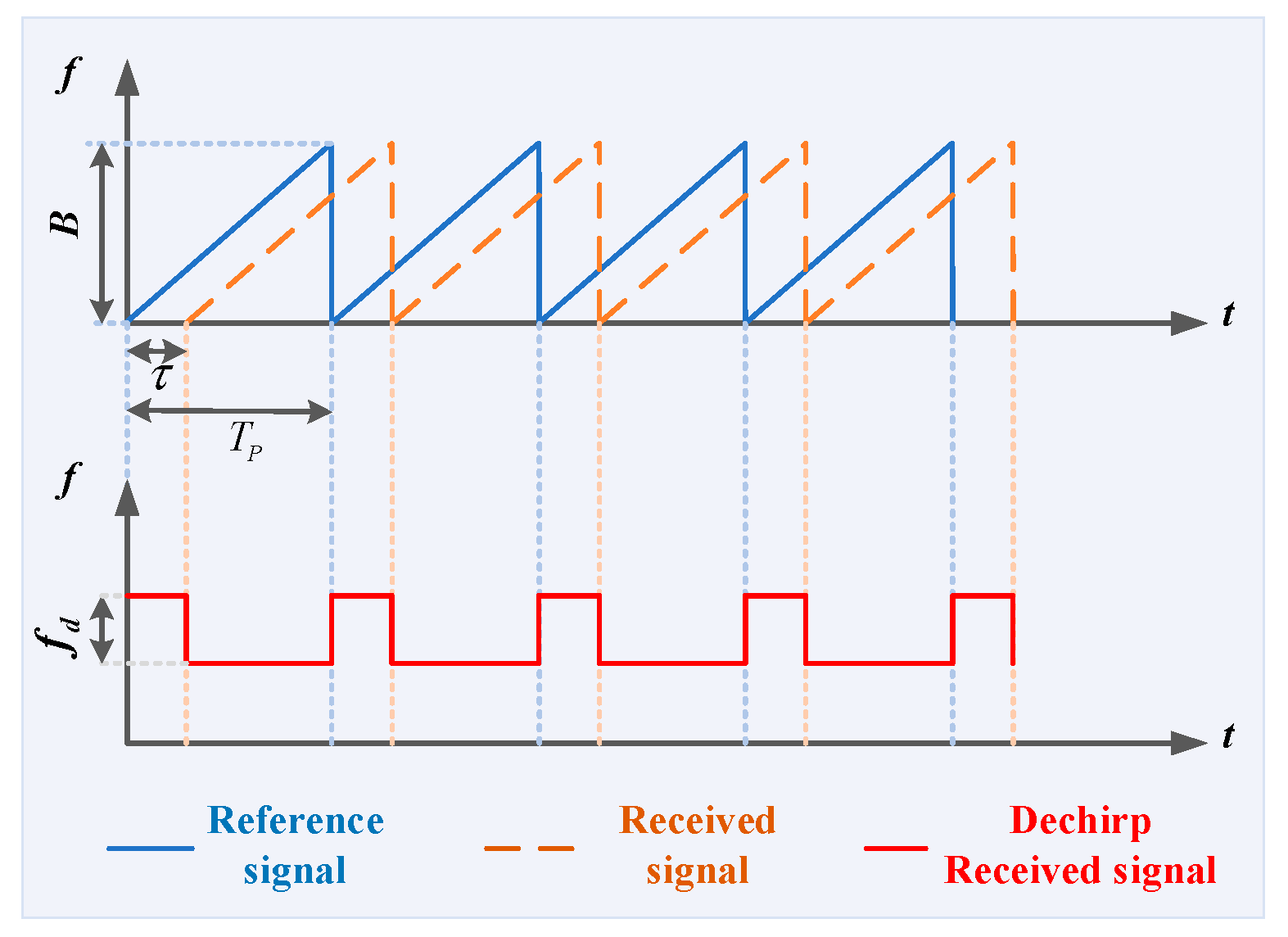
Considering that laser-radar signals have a wide bandwidth and the observed scenes are relatively small, the dechirping processing can effectively reduce the sampling rate. We can take the sawtooth FMCW as an example, as shown in Figure 2. The blue line represents the time–frequency curve of the reference signal, the dashed orange line represents the time–frequency curve of the received signal, and the red line represents the time–frequency curve of the dechirp received signal. Observing Figure 2, T P represents the pulsewidth, f = 1 / T P is the sweep frequency, and B is the bandwidth. τ represents the time interval between the transmission of the signal from the radar system and its reception by the radar detector after reflection from the target, τ = 2 R / c . R represents the range between the target and radar. c represents the speed of light.
Assume that the transmission signal of the laser radar is linearly frequency-modulated (LFM):
s t = rect t T P exp j 2 π f c t + 1 2 γ t 2
where rect [ ] is the rectangular window function, t represents the fast time. f c represents the carrier frequency, and γ is the chirp rate of the signal.
If the target is composed of P scattering points, the range from the i-th  1 i P scattering point to the radar is R i , and the target echo signal received by the radar is
s r t = i = 1 P a i rect t 2 R i c T P exp j 2 π f c t 2 R i c +   j π γ t 2 R i c 2
where a i represents the reflectivity coefficient corresponding to the i-th scattering point.
The reference signal is
s r e f t = rect t 2 R r e f c T r exp j 2 π f c t 2 R r e f c + j π γ t 2 R r e f c 2
where R r e f represents the reference range. T r represents the pulsewidth of s r e f t , which is longer than T P .
s d t = s r t s r e f t   = i = 1 P a i rect t 2 R i c T P exp j 4 π c γ t 2 R r e f c R i Δ exp j 4 π c f c R i Δ exp j 4 π γ c 2 R i Δ 2
where R i Δ = R i R r e f , and [ ] represents conjugate operation. Applying the Fourier transform to Equation (4), we can obtain the range profile of laser radar, which can be expressed as
S d f = i = 1 P a i sin c T P f + 2 γ c R i Δ   exp j 4 π c f c R i Δ exp j 4 π γ c 2 R i Δ 2 exp j 4 π f R i Δ c
Observing Equation (5), the dechirp-received signal becomes a narrow pulse in the shape of a sinc function with a width of T P and its peak is located at f = 2 γ × R i Δ / c in the frequency domain. We can obtain the range from the target to the laser radar through the position of this narrow pulse.
R i Δ = c f 2 γ
The range resolution can be written as
ρ = c 2 γ × 1 T P = c 2 B
If the observation range of the laser radar is Δ R , then the frequency range after the dechirping is Δ R × γ / c , Δ R × γ / c , and the bandwidth of the dechirp-received signal can be expressed as
f d = 2 Δ R c γ
After dechirp reception, the bandwidth of the dechirp received signal decreases significantly compared to the original signal. Effective sampling of the dechirp received signal can be achieved when the sampling frequency is greater than twice the highest frequency of the dechirp-received signal.
F s 2 Δ R c γ
Here, F s denotes the Nyquist sampling frequency of the dechirp-received signal.

2.2. Ranging Model Based on the Multi-Channel Coprime Low-Sampling Scheme

Although the sampling rate can be reduced by dechirp operation, it still faces challenges of high-speed sampling and high data storage when dealing with wide bandwidths and expansive scenes. To address this issue, this manuscript proposes the multi-channel coprime low-sampling scheme. The sampling rate remains constant within each channel, while the intervals among channels are coprime. Compared to random sampling, the proposed method has a simpler hardware implementation.
The transformation of the dechirp-received signal from the time domain to the frequency domain can be discretely expressed [25,26,35] as
s = F a
where F is the inverse Fourier basis matrix. a is the range profile, which corresponds to the frequency-domain vector of the dechirp-received signal and has strong sparsity. s is observation vector of the dechirp-received signal in the time domain.
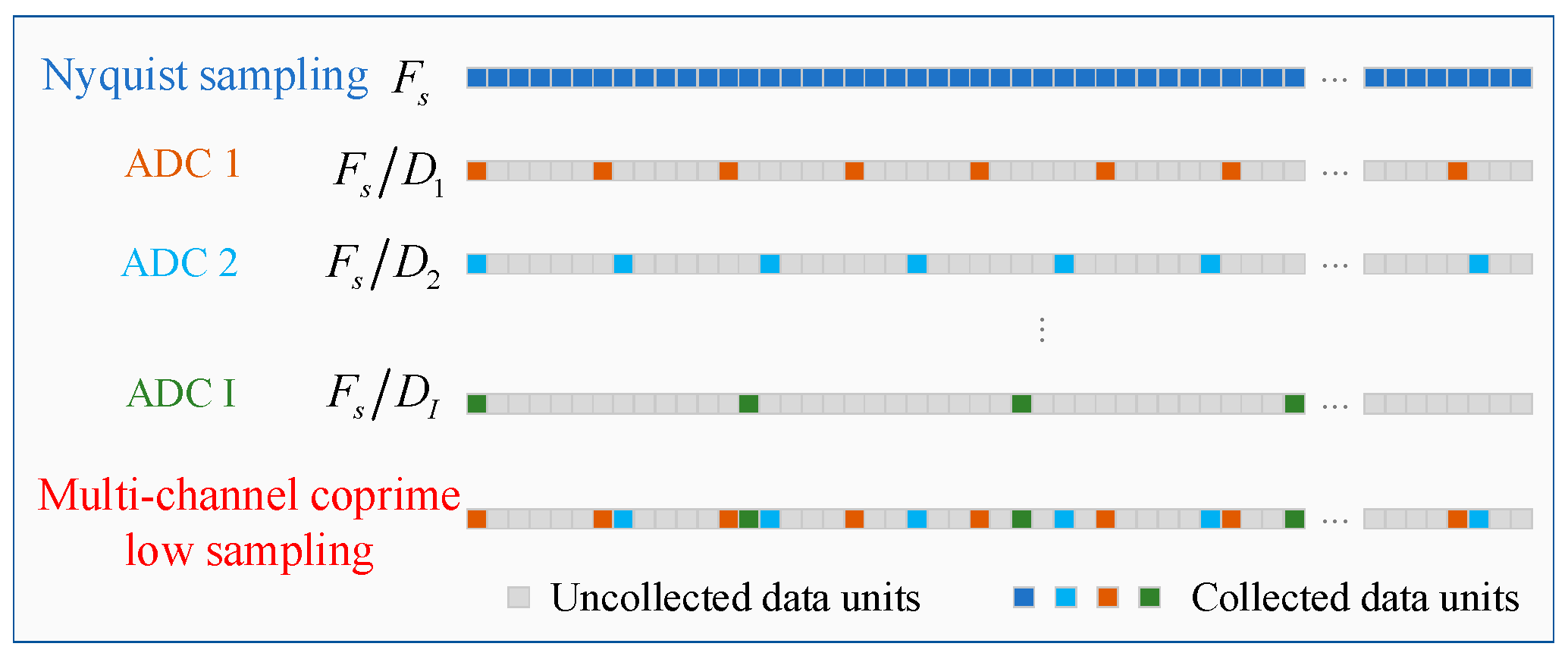
The multi-channel coprime low-sampling scheme is shown in Figure 3. There are I coprime multiple channels, and each channel has a fixed sampling frequency. The sampling intervals among channels are uniform and coprime. The sampling rates of each channel ADC are F s / D 1 , F s / D 2 , F s / D I , where F s is the Nyquist sampling rate of the laser radar, and D 1 , D 2 , , D I are all coprime. The sum of the sampling rates of multi-channel coprime low-sampling is less than F s . s i M i × 1 is the time-domain echo of the dechirp-received signal that can be collected by the i th channel, where 1 i I . M is the number of sampling points of laser radar under ideal Nyquist sampling.
The signals collected by the multi-channel coprime low-sampling can be expressed as
s M C O = Φ M C O a + n s M C O = Γ v e c s 1 , s 2 , , s I T M ¯ × 1 Φ M C O = Γ Φ 1 , Φ 2 , , Φ I T M ¯ × M Φ i = Φ i 1 , Φ i 2 , Φ i M i , Φ i M M i × M 1 i I Φ i n = Φ i n , 1 , Φ i n , 2 , Φ i n , M i , Φ i n , M 1 n M i Φ i n , m = exp j 2 π n 1 D i m M 1 m M
where s M C O represents the pre-processed echo after the dechirping of the multi-channel coprime low-sampling scheme. a is the range profile to be reconstructed. n is the system noise, and Φ M C O is the sensing matrix of the multi-channel coprime low-sampling, which is the non-uniform Fourier transform matrix. In Equation (11), s i and Φ i represent echo under dechirp processing and partial sensing matrix of the i-th channel. Γ · represents the matrix operation, which sorts the data according to the acquisition time and eliminates the repeated acquisition values of multi-channels at the same time. After the above matrix operation on data from the multi-channel coprime low-sampling scheme, s M C O is the M ¯ × 1 matrix, Φ M C O is the M ¯ × M matrix, and M ¯ < i = 1 I M i . In the model-establishment process, we can see that the sample number based on the multi-channel coprime low sampling is much smaller than the Nyquist sampling.
When ADC based on the multi-channel coprime low-sampling scheme performs laser-radar sampling, there is asynchronous sampling-time error among the channels. The model is as follows:
s M C O _ g = Φ M C O _ g a + n = Θ Φ M C O a + n
where s M C O _ g represents the echo after the dechirping process of the multi-channel coprime sampling with sampling-time error, Θ is the phase-error matrix of the sampling-time error, and represents the Hadamard product.

3. High-Resolution Ranging Based on Optimal Multi-Channel Coprime Low-Sampling under Low SNR

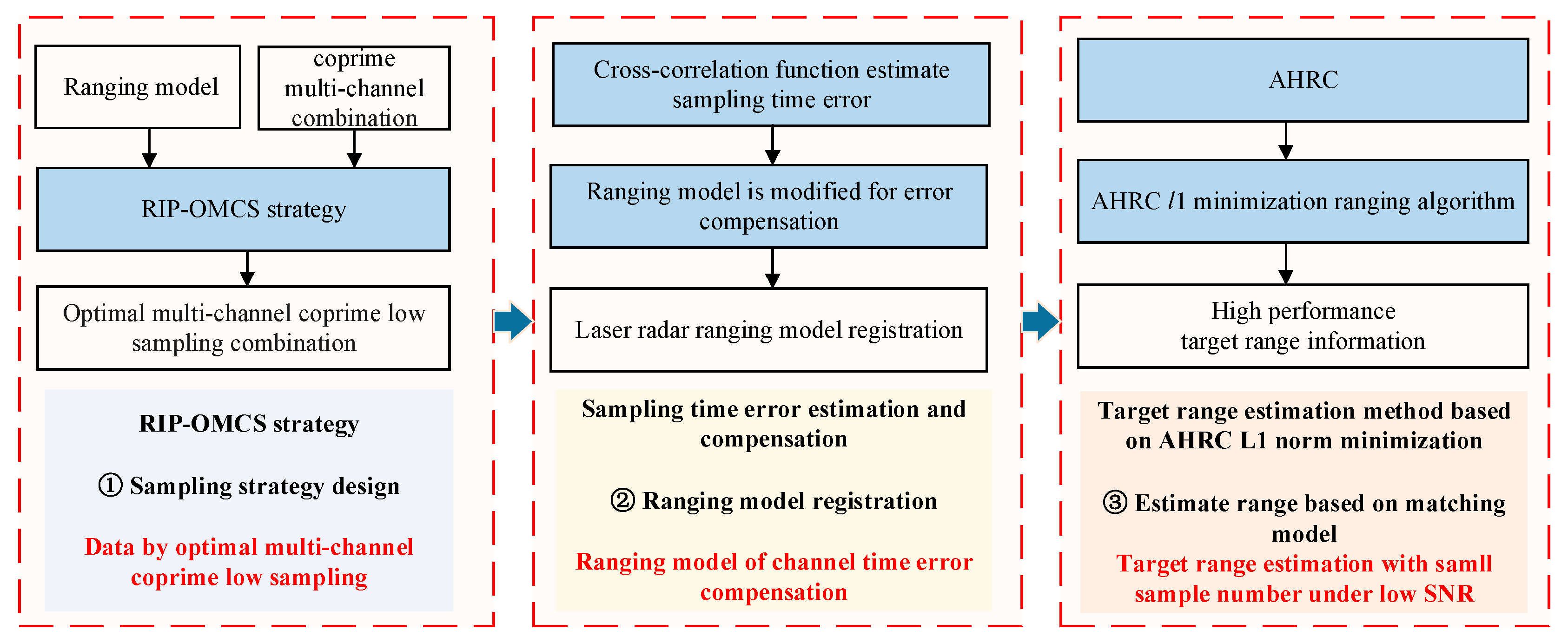
High-resolution ranging based on optimal multi-channel coprime low-sampling under low SNR is proposed in this section, and some key procedures are discussed in detail. According to the ranging model in Section 2, the challenges of selecting the optimal multi-channel coprime low-sampling combination and mitigating asynchronous sampling-time error and noise interference are crucial for accurately estimating the target range with a small sample number. To address these issues, in this manuscript, we propose the novel processing framework shown in Figure 4.
  • To reduce the overall sample number of the laser-radar system, we propose the RIP-OMCS strategy. This strategy achieves a small overall sample number while maintaining ranging accuracy.
  • Addressing the issue of asynchronous sampling-time error, we propose the cross-correlation method to estimate errors. The time error compensation is performed by means of ranging model registration.
  • To tackle the performance limitations of traditional sparse-reconstruction algorithms and the accuracy issues of target-range estimation under low SNR, we introduce a target-range estimation method based on AHRC l 1 minimization under a low SNR. AHRC is formulated by combining logarithmic and arctangent penalty functions. This constraint function dynamically imposes precise constraints on the noise and target components, obtaining a high-resolution range profile and enhancing the target-range-estimation accuracy.

3.1. RIP-OMCS Strategy

Nyquist sampling may lead to a large amount of data transmission and storage requirements, increasing system cost and complexity. According to the model established in Section 2, this section proposes the RIP-OMCS strategy, which can significantly reduce the sample number while ensuring the ranging accuracy.
Assume that the range profile a M contains at most K non-zero elements, where M represents the space of complex numbers. Then, a is referred to as K-sparse [19], denoted as
a K = a M : a 0 K
where · p is the l p norm.
Since the range profile is sparse, we can use compressed sensing to process sparse signals, which can achieve high-precision estimation of target-range information with fewer data. If the sparse sampling strategy satisfies the RIP [20,53,54], the accurate estimation of the range can be obtained under the minimum number of samples. The general sampling method can be described by the sensing matrix. In Section 2, the sensing matrix Φ M C O is a non-uniform Fourier transform matrix, so Φ M C O should meet the RIP. For any K-sparse range profile, the following conditions should be satisfied
1 δ K a 2 2 Φ M C O a 2 2 1 + δ K a 2 2
where δ K is the K-order Restricted Isometry Coefficient (RIC), and its value range is 0 δ K 1 . The RIP ensures that the sensing matrix does not map different sparse signals to the same target-range unit.
The non-uniform Fourier transform matrix Φ M C O can be regarded as a dimensionality-reduction operator. If Φ M C O satisfies the RIP, the measurement is accurate enough, and the original signal is a sparse signal. Equation (12) has a unique exact solution. For any K-sparse laser-radar range profile a , let τ be its support set; then, we can obtain the following:
Φ M C O a 2 2 = Φ M C O τ a , Φ M C O τ a = Φ M C O τ H Φ M C O τ a , a
where · is the scalar product, and · H denotes conjugate transpose. If Φ M C O satisfies the RIP, then the eigenvalues of Φ M C O τ H Φ M C O τ belong to 1 δ K , 1 + δ K . The smaller δ K is, the closer the eigenvalue of Φ M C O τ H Φ M C O τ is to 1, which means that Φ M C O τ H Φ M C O τ is closer to the unit matrix. This shows that the column vectors of Φ M C O are approximately orthogonal to each other, and the equation group (12) composed of the laser-radar ranging model based on a multi-channel coprime low-sampling scheme is independent. A more accurate target-range estimation result is obtained by solving this equation group.
In this manuscript, the optimal RIC is used as the RIP-OMCS strategy for the selection of a multi-channel coprime low-sampling combination. The selected optimal coprime multiple channels can significantly reduce the required sample number while maintaining high-quality signal acquisition. This provides data support for the high-performance sparse reconstruction of target-range information.

3.2. Asynchronous Sampling-Time Error Estimation and Compensation

The performance of hardware implementation components may constrain the sampling time of different channel ADCs. Asynchronous sampling-time errors can lead to mismatches in the ranging model, failing to reconstruct the range profile. In Section 3.2, the mathematical model analyzes the influence of sampling-time errors of the coprime channels, and sampling-time errors are estimated by the cross-correlation function.
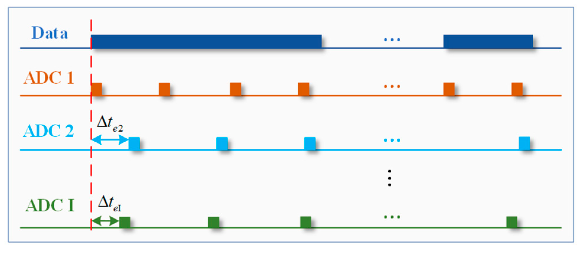
The sampling-time error is a fixed synchronization time error, as shown in Figure 5. When the channel has a sampling-time error Δ t e , the signal received by the channel can be expressed as
s r _ e t + Δ t e = i = 1 P a i rect t + Δ t e 2 R i c T P exp j 2 π f c t + Δ t e 2 R i c exp j π γ t + Δ t e 2 R i c 2
The dechirp-received signal with a sampling-time error can then be obtained
s d _ e t + Δ t e = i = 1 P a i rect t + Δ t e 2 R i c T p exp j 4 π c γ t + Δ t e 2 R r e f c R i Δ exp j 4 π c f c R i Δ   exp j 4 π γ c 2 R i Δ 2
Fourier transform is performed on Equation (17), and the frequency-domain expression of the dechirp-received signal with sampling-time error can be obtained
S d _ e f = i = 1 P a i sin c T P f + 2 γ c R i Δ exp j 4 π c f c R i Δ exp j 4 π γ R i Δ 2 c 2 exp j 4 π f R i Δ c exp j 2 π f c Δ t e
It can be seen in Equation (18) that the dechirp-received signal with sampling-time error from the time domain to the frequency domain becomes a sinc-shaped narrow pulse with a width of 1 / T p and a peak value at f = 2 γ × R i Δ / c . It is obvious that the peak position is not affected by the sampling-time error. However, the phase in the frequency domain will change, and the change is related to the sampling-time error Δ t e . Due to the phase error of the dechirp-received signal between the channels, the dechirp-received signal among the channels will degenerate into a non-coherent signal, and it is impossible to combine multiple channels to achieve high-precision signal recovery.
To solve these problems, Section 3.2 proposes a sampling-time error estimation method based on cross-correlation function, which is shown in Figure 6.
Assuming that the sampling-time error is independent of time, the calibration signal can be used to estimate sampling-time error, and the bandwidth of the calibration signal is less than the minimum channel sampling frequency in the optimal multi-channel coprime low-sampling combination. The signal spectrum after the dechirping process is S i 1 i I O , and I O is the total number of channels. The dechirp-received signal spectrum is interpolated and truncated, so that the spectrum range and sampling points of each channel are consistent, and the corresponding spectrum is u i . The corresponding time-domain spectrum u t _ i is further obtained. The first ADC sampling channel is used as the reference channel, and the cross-correlation function of the time-domain spectrum of the i-th channel and the reference channel can be expressed as
R 1 i τ Δ i = u t _ 1 t u t _ i t τ Δ i d τ Δ i 1 < i I O
According to the value of R 1 i τ Δ i , the coarse sampling-time error Δ t m i can be estimated. However, the coarse sampling-time error estimated by Equation (19) is the multiple of the sampling time. The sampling rate of each channel is relatively low, and the sampling-time error-estimation accuracy is also poor. In order to improve the accuracy of sampling-time error estimation, the target phase in each channel spectrum can be used to estimate the small sampling-time error, which can be expressed as
u i f = u 0 _ i f exp j 2 π f Δ t s i
where u 0 _ i is the spectrum obtained by interpolating and truncating the dechirp-received signal spectrum of each channel when there is no sampling-time error. The small sampling-time error estimation results Δ t s i in the range of π , π can be estimated from the phase angle u i f . Using the small sampling-time error Δ t s i , combined with the coarse sampling-time error Δ t m i of phase ambiguity eliminating, we can obtain the precise sampling-time error Δ t e i corresponding to the i-th coprime channel and the reference channel.
According to the phase-error factor of Equation (20), the laser-radar ranging model is registered. The ranging model under sampling-time error compensation is obtained as follows:
s M C O _ g = Φ M C O _ g a + n = Θ Φ M C O a + n s M C O _ g = Γ v e c s g 1 , s g 2 , , s g I T M ¯ × 1 Θ = Γ Θ 1 , Θ 2 , , Θ I O T M ¯ × M Θ i = Θ i 1 , Θ i 2 , Θ i n , Θ i M M i × M 1 i I O Θ i n = Θ i n , 1 , Θ i n , 2 , Θ i n , M i , Θ i n , M 1 n M i Θ i n , m = exp j 2 π Δ t e i F S M m 1 m M
where s M C O _ g represents the echo based on the multi-channel coprime low-sampling scheme with sampling-time error, and s g i is the echo under dechirp processing of the i-th channel with the sampling-time error. Θ is the phase-error matrix of the sampling-time error.

3.3. AHRC l 1 Minimization for Target-Range Estimation

After asynchronous sampling-time error compensation, the measurement data of the multiple channels can be combined so that the target-range estimation can be converted into the high-precision frequency-estimation problem of the non-uniformly sampled signals. It is necessary to break through the limited length of data observation and non-uniform sampling to complete ultra-high-precision frequency analysis. At the same time, due to the decrease in the amount of sampling data, the coherent accumulation value of the target signal becomes lower, which makes the influence of environmental noise more obvious. Thus, it is more critical to suppress the influence of noise.
Based on the ranging model obtained in Section 3.2, this section proposes an AHRC l 1 minimization target-range estimation method combining the logarithmic penalty function and arctangent penalty function.
Solving Equation (21) can realize the high-resolution range-profile reconstruction and target-range estimation under the optimal coprime low-sampling multi-channel scheme. The optimization problem of Equation (21) can be written as
min a 1 ,   s . t .   s M C O _ g = Θ Φ M C O a + n
By solving the optimization problem of Equation (22), the reconstructed laser-radar range profile can be obtained, and the target range can be estimated. However, the performance of the target-range estimation obtained by directly solving Equation (22) is limited under the condition of a low SNR. To improve the accuracy of target-range estimation under a low SNR, it is necessary to use l 1 weighting [35,55,56] and prior knowledge to ensure that the parameters converge to the actual value.

3.3.1. AHRC

The effective weighted l 1 can distinguish the contribution of signal and noise on the ranging model, improve the reconstruction performance of the range profile at a low SNR, and make the target-range-estimation result more accurate at a low SNR. The weighted l 1 optimization problem can be expressed as
min W a 1 ,   s . t .   s M C O _ g = Θ Φ M C O a + n
where W is the weight diagonal matrix; the weight of the i-th component of a on the diagonal is w i , and the others are zero. In the weighted l 1 norm optimization problem of Equation (23), it is necessary to select the appropriate weighting coefficient to make the solution as small as possible to satisfy the sparsity. More importantly, the non-zero part of the solution is consistent with the target amplitude and position, and the zero part of the solution corresponds to the noise, which can make the recovery result more accurate. Applying a large constraint coefficient to the element in the solution can make the element reach a zero value. On the contrary, applying a small constraint coefficient can make the element reach a non-zero value, and the value of the non-zero value is still affected by the constraint coefficient. Therefore, how to establish the mapping relationship between the constraint coefficient and the element values of the results to be restored determines the accuracy of the recovery results. The constraint coefficient needs to be determined by the solution, and the solution is unknown in the process of completing the solution, which means the solution of Equation (23) can only be completed by the Expectation Maximization (EM) algorithm. We must gradually correct the constraint coefficient of the solution according to the change of the solution in the iterative solution process. In the iterative process, the re-weighted constraint of the solution is updated, and the function describing the relationship between the solution and the constraint coefficient cannot be simply constructed by the inverse ratio of the solution. It should have sufficient sensitivity to the numerical changes of the solution and have the rationality of change mapping so that the constraint coefficient can converge to the most appropriate value in the iterative process to ensure the rationality and accuracy of the solution.
Both the logarithmic function and arctangent function have the trend wherein the slope tends to zero when the independent variable increases. The logarithmic function is such that as the independent variable increases, the slope gradually approaches 0. The arctangent function is such that as the independent variable increases, the slope can quickly approach 0, but the slope of the logarithmic function is greater than that of the arctangent function when the independent variable is very small. Therefore, this manuscript proposes a hybrid re-weighted constraint coefficient construction method combining the logarithmic penalty function and arctangent penalty function by using the characteristics of the logarithmic penalty function and arctangent penalty function under different independent variables.
The arctangent penalty function is used to construct weights; Equation (23) can be expressed as
min m = 1 M a r c tan a m ε , s . t .   s M C O _ g = Θ Φ M C O a + n , m = 1 , M
where a m is the m-th component of a , ε > 0 . Equation (24) can then be rewritten as
min m = 1 M a r c tan u m ε , s . t .   s M C O _ g = Θ Φ M C O a + n ,   a m u m
These formulas show that if a is the solution of Equation (24), a , a is the solution of Equation (25); conversely, if a , u is the solution of Equation (25), then a is the solution of Equation (24).
u k and a k are the k-th iteration result of the optimization variable. The first-order Taylor expansion of m = 1 M a r c tan u m ε can be expressed as
m = 1 M a r c tan u m ε m = 1 M a r c tan u m k ε + m = 1 M u m u m k u m k 2 + ε 2 ε
Through deduction, we can obtain
a k + 1 , u k + 1 = arg min m = 1 M u m u m k 2 + ε 2 , s . t .   s M C O _ g = Θ Φ M C O a + n ,   a m u m
where u m k is the m-th component of u k . a m k is the m-th component of a k . It can be rewritten as
a k + 1 = arg min m = 1 M a m a m k 2 + ε 2 , s . t .   s M C O _ g = Θ Φ M C O a + n
The arctangent penalty function can determine that the re-weighted matrix of a in the k-th iteration is
W a r c tan k = d i a g a m k 2 + ε 2 1
The logarithmic penalty function [55] is used to construct the reweighted weights W log k , and Equation (23) can be expressed as
min m = 1 M log a m + ε , s . t .   s M C O _ g = Θ Φ M C O a + n
By repeating the Equations (24)–(28) deduction process, the logarithmic penalty function constructs the reweighted matrix W log k = d i a g a m k + ε 1 of a in the k-th iteration.
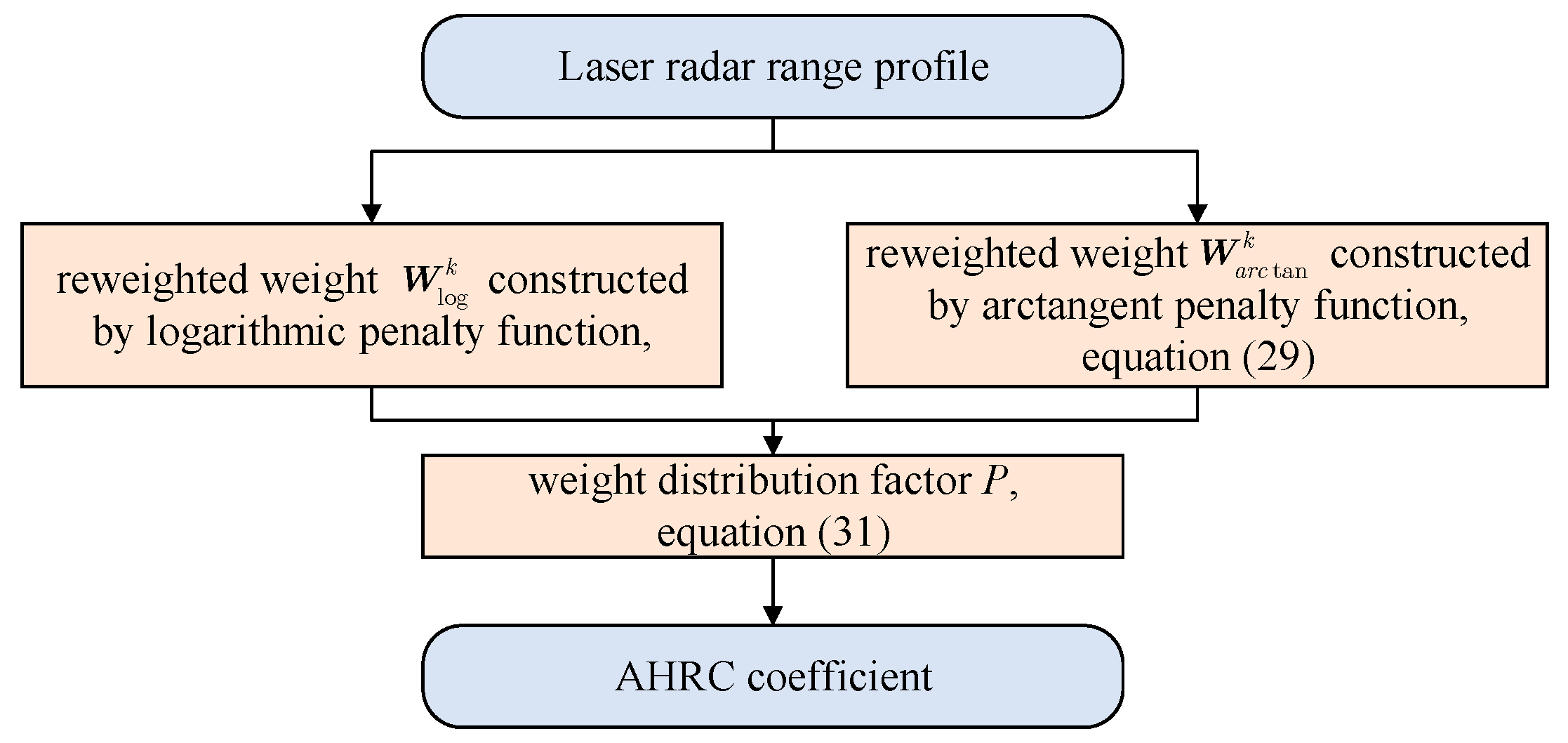
When a m k is small, the logarithmic penalty function performs better, and when a m k is large, the arctangent penalty function performs better. The weight distribution factor P is introduced to construct the AHRC matrix W .
P m k = a m k max a m k + C
w m k = 1 a m k 2 + ε 2 × P m k + 1 a m k + ε × 1 P m k
Here, P m k represents the weight-distribution factor of the a m k , and the larger the value of a m k , the larger the value of P m k . C > 0 is the weight-balance coefficient. w m k is the AHRC coefficient corresponding to a m k .
The flowchart of AHRC is shown in Figure 7. In this manuscript, ε is considered to be one-thousandth of the average absolute value of the distance image, and the weight-balance coefficient C is the average absolute value of the profile range. As shown in Figure 7, AHRC adopts a complex weighting scheme, which adds a smaller weight to the strong-scattering center region and a bigger weight-to-noise region. Combined with the characteristics of the logarithmic penalty function and the arctangent penalty function in different regions, AHRC can better distinguish the influence of signal and noise on solving the optimization problem, reconstruct the target distance more accurately, and reduce the influence of noise in the solution process. In addition, the strategic allocation of weights enables AHRC to dynamically adapt to changing SNR and ensure robust performance under different scenarios and environmental conditions.

3.3.2. Statistical Modeling

In this section, maximum a posteriori (MAP) estimation [22,23] is used to transform the laser-radar ranging model based the optimal multi-channel coprime low-sampling scheme into the sparse representation problem. The complex Gaussian model is used to represent the noise distribution [22,26]. The weighted range profile W a submits to the Laplace distribution, and the elements are independent of each other and submit to the same distribution [23].
P D F s M C O _ g W a = π σ n 2 M exp 1 σ n 2 s M C O _ g Θ Φ M C O W 1 W a 2 2
P D F W a γ = γ 2 M exp γ W a 1
Here, σ n 2 is the variance of n . γ is the Laplace scale coefficient. Using the MAP estimation, the final formulation is decomposed into the iteration between the sparse reconstruction of the target range and the AHRC:
a ^ = arg min a s M C O _ g Θ Φ M C O a 2 2 + μ W a 1
W = F W a ^
where μ represents the sparse-constraint coefficient, which is determined by the variance and image distribution of the laser-radar range profile. The previous section analyzes the relationship between W and a , which can be expressed by the function F W · .
The sparse-constraint coefficient μ is the parameter used to measure the fidelity and sparsity of the signal. It can effectively suppress the influence of scene noise when it is used in Equation (35), which can be expressed as
μ = σ 2 γ σ 2 = E a n o H a n o γ = M / a 1
where E · denotes the averaging operation. The noise unit is extracted from the laser-radar ranging profile and vectorized to obtain the noise vector a n o .
The proposed method transforms the laser-radar ranging into the MAP estimation of sparse constraints using the Laplace distribution to describe the target signal and considering the noise of the complex Gaussian distribution. Using statistical modeling, we can quantify the sparsity and noise of the target signal and accurately select the parameters in the sparse optimization. The sparse-constraint coefficient depends entirely on the statistical parameters of the target signal and noise, and the mathematical meaning is clear. It addresses a common challenge encountered in many existing l 1 regularization methods, where the selection of sparse-constraint coefficients poses difficulty and the mathematical interpretation remains unclear. At the same time, AHRC can better distinguish the influence of signal and noise when solving the optimization problem, reconstruct the target range more accurately, and reduce the influence of noise on the solution process. By using μ and W , a high-resolution range profile and better target-range-estimation results can be achieved at a low SNR.

3.3.3. Solution of the Optimization Problem

The laser-radar ranging of RIP-OMCS is transformed into the sparse solution problems of AHRC l 1 minimization in Equations (35) and (36). The quasi-Newton method and conjugate gradient method are used to solve the problem.
W k = d i a g 1 a m k 2 + ε 2 × P m k + 1 a m k + ε × 1 P m k
H a k = Θ Φ M C O H Θ Φ M C O + μ W k Λ a ^ k
H a k a ^ k + 1 2 Θ Φ M C O H s M C O _ g = 0
Here, a ^ k and a ^ k + 1 are the estimates of a in the k-th and (k + 1)-th iterations, respectively. W k is the AHRC coefficient corresponding to a ^ k . H a k is an approximated Hessian matrix. Λ a ^ k is the diagonal matrix, and its m-th element is a ^ m k 2 + τ 1 / 2 , where τ is a constant small positive number used to overcome the non-differentiability of a ^ m k .
The conjugate gradient method [23] is used to solve Equation (40), which can effectively avoid the high amount of computation caused by matrix inversion in the optimization iteration. The solution of the conjugate gradient method can obtain the reconstructed laser-radar range profile a ^ k + 1 at the (k + 1)-th iteration and through several iterations until the convergence condition a ^ k + 1 a ^ k 2 / a ^ k 2 ρ is satisfied, where ρ represents the preset threshold.
The target-range-estimation method based on AHRC l 1 minimization is shown in Figure 8. The sparse-constraint coefficient μ and the AHRC coefficient W suppress the influence of noise on target-range information estimation in the process of solving and can reconstruct the high-resolution range profile and obtain high-accuracy target-range information under a low SNR.

4. Discussion

In this section, we conduct experiments on different situations of data to verify the effectiveness of the proposed method. For further comparative analysis, various types of methods are used as reference comparison methods [25,57].

4.1. Performance Analysis of RIP-OMCS

This section describes the experiments carried out based on laser-radar data to verify the effectiveness of RIP-OMCS. Assume that the laser radar transmits an LFM signal with the parameters shown in Table 1. The selected multi-channel coprime low-sampling combination is shown in Table 2. There are three sets of coprime multi-channel combinations. The down-sampling rate is the ratio of the sample number of the coprime combination to the number of Nyquist samplings.
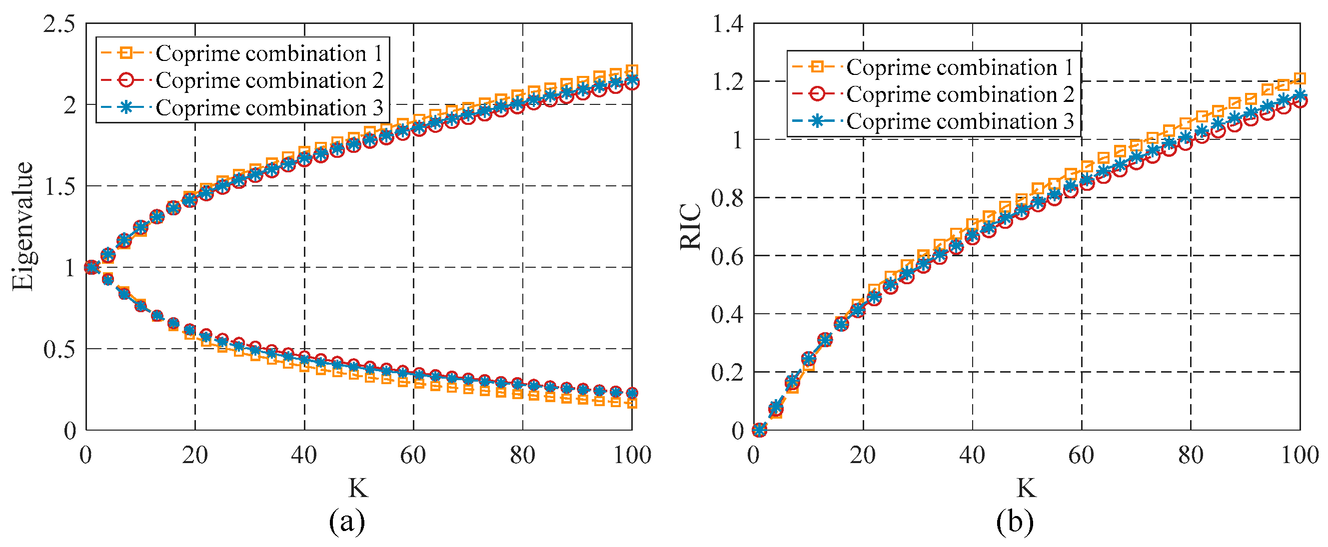
The performance of the different coprime combinations is shown in Figure 9. Under the sensing matrix of each coprime combination, the number of strong points K was traversed from 1 to 100, and 5000 random experiments were performed under each K. Figure 9a shows the maximum and minimum eigenvalue corresponding to the coprime combination, and Figure 9b shows the RIC corresponding to the coprime combination. The RIC of Coprime Combination 2 was the smallest, and its performance was the best. Therefore, based on the RIP-OMCS strategy, Coprime Combination 2 was selected as the optimal multi-channel coprime combination for the following analysis.
In the experimental process, qualitative and quantitative indicators were used to objectively evaluate the proposed algorithm. The correlation coefficient (CORR) [26,57] was used to evaluate the target-range-estimation performance of multi-channel coprime low-sampling. CORR reflects the similarity between two radar-range profiles, which is expressed as
CORR = a 0 , a ^ a 0 2 · a ^ 2
where a 0 and a ^ are the complex vectors. a 0 and a ^ are the radar range profiles from the ideal reference Nyquist sampling and sparse-reconstructed data, respectively.
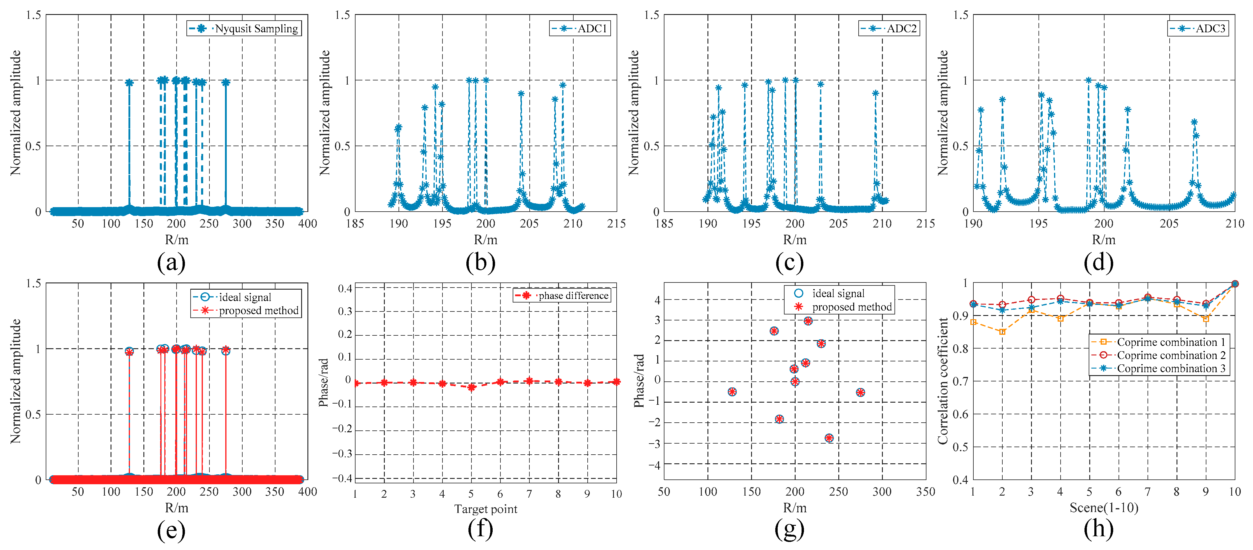
Figure 10 shows the comparative analysis of the results of the optimal coprime combination. In this manuscript, ε is considered to be one-thousandth of the average absolute value of the distance image, and the weight-balance coefficient C is the average absolute value of the profile range. Figure 10a is the range profile under the ideal Nyquist sampling. Figure 10b–d are the range profiles under each channel. Figure 10e shows the comparison of the radar-range profiles between the sparse reconstruction using the proposed method and the ideal Nyquist sampling. Figure 10f shows the target phase difference between the ideal Nyquist sampling and the proposed method. Figure 10g shows the two-dimensional comparison of target-range information and target-phase information between the sparse reconstruction using the proposed method and the ideal Nyquist sampling. Figure 10h shows the correlation-coefficient comparison of 3 coprime combinations in 10 scenarios (different target positions in the scene). Figure 10 shows that the proposed method can effectively reconstruct the target-range profile with a small sample number. It is worth noting that the reconstructed target position and phase have very high fidelity in the target position and phase obtained by Nyquist sampling, indicating the excellent accuracy and reliability of the range-estimation method based on AHRC l 1 minimization. The selected optimal Coprime Combination 2 had the best performance in multiple scenarios. This further verifies the reliability and effectiveness of the RIP-OMCS strategy. The RIP-OMCS strategy can select the optimal multi-channel coprime low-sampling combination, which can effectively use low-sampling data to reconstruct a high-resolution radar-range profile, expand the radar ranging range, and obtain accurate target-distance information. In addition, the proposed method helps to save data sampling and storage resources, thereby improving operational efficiency and effectiveness, and the internal sampling of each channel is uniform and easy to implement on hardware.

4.2. Performance Analysis of Sampling-Time Error Compensation

To verify the effect of the sampling-time error compensation method, we now show the sampling-time error-compensation results of the optimal multi-channel coprime low-sampling combination. Figure 11 compares the results before and after the sampling-time error compensation of the optimal multi-channel coprime low-sampling combination. Figure 11a compares the radar range profile between the sparse reconstruction using the proposed method with sampling-time error compensation and the ideal Nyquist sampling. Figure 11b compares the radar range profile between the sparse reconstruction using the proposed method without sampling-time error compensation and the ideal Nyquist sampling. Figure 11c shows a two-dimensional comparison of target range information and target phase information under sampling-time error compensation, without sampling-time error compensation and ideal sampling. Figure 11d shows the correlation-coefficient comparison between sampling-time error compensation and without compensation sampling-time error in 10 scenarios.
It can be clearly seen that there was a mismatch in the ranging model with sampling-time error, and the obtained ranging result had a large deviation from the ideal range and phase. The sampling-time error estimation and compensation method proposed in this manuscript can effectively reduce the impact of sampling-time error. The proposed method can effectively register the ranging model, and the target-range estimation performance of the compensating sampling-time error is excellent, which is much better than that of without compensated sampling-time error.
To verify the robustness of the sampling-time error-estimation and compensation method, we performed Monte Carlo tests to test the target-distance-estimation performance under different scenarios and different sampling-time error conditions, and 100 random scene experiments were performed under each sampling-time error. Figure 12 shows the average of the correlation coefficients of different sampling-time errors between the compensated sampling-time error and the without compensated sampling-time error. The performance of the target-range estimation with sampling-time error compensation is much better than that without sampling-error compensation. The correlation coefficient also proves that the proposed method is robust.

4.3. Performance Analysis of the Proposed Algorithm under Different SNRs

To verify the performance of the target-range-estimation method based on AHRC l 1 minimization under different SNRs, white Gaussian noise was added to the echo to generate different SNR echo data.
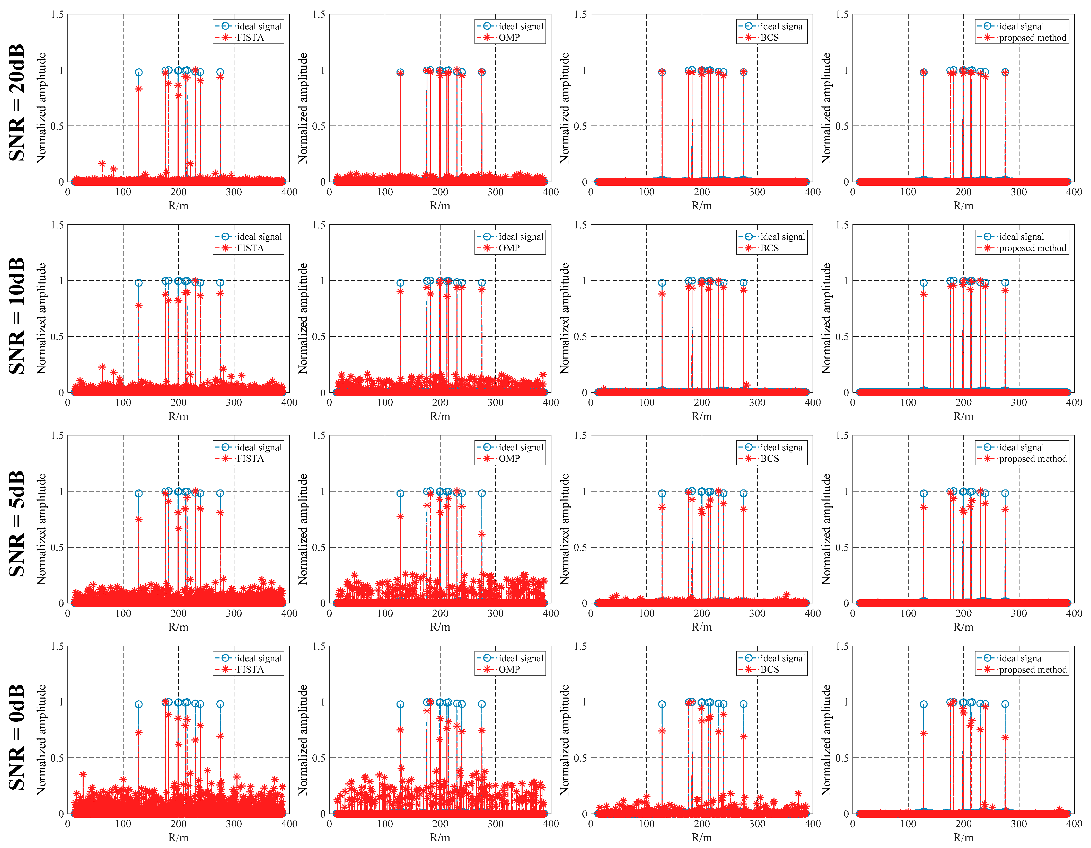
Figure 13 shows different algorithms’ target-range-estimation results when the SNR is 20, 10, 5, and 0 dB, respectively. The target-range information obtained by the FISTA algorithm is shown in the first column in Figure 13. The target-range information obtained by the OMP algorithm is shown in the second column in Figure 13. The target-range information obtained by the BCS algorithm is shown in the third column in Figure 13. The target-range information obtained by the proposed method is shown in the fourth column in Figure 13. When the SNR is 20 dB, the target-range information can be obtained by the four algorithms. With the continuous reduction in the SNR, the target-range estimation results of OMP, FISTA, and BCS algorithms have strong false points. The proposed method can still accurately obtain the target-range information without introducing strong false points.
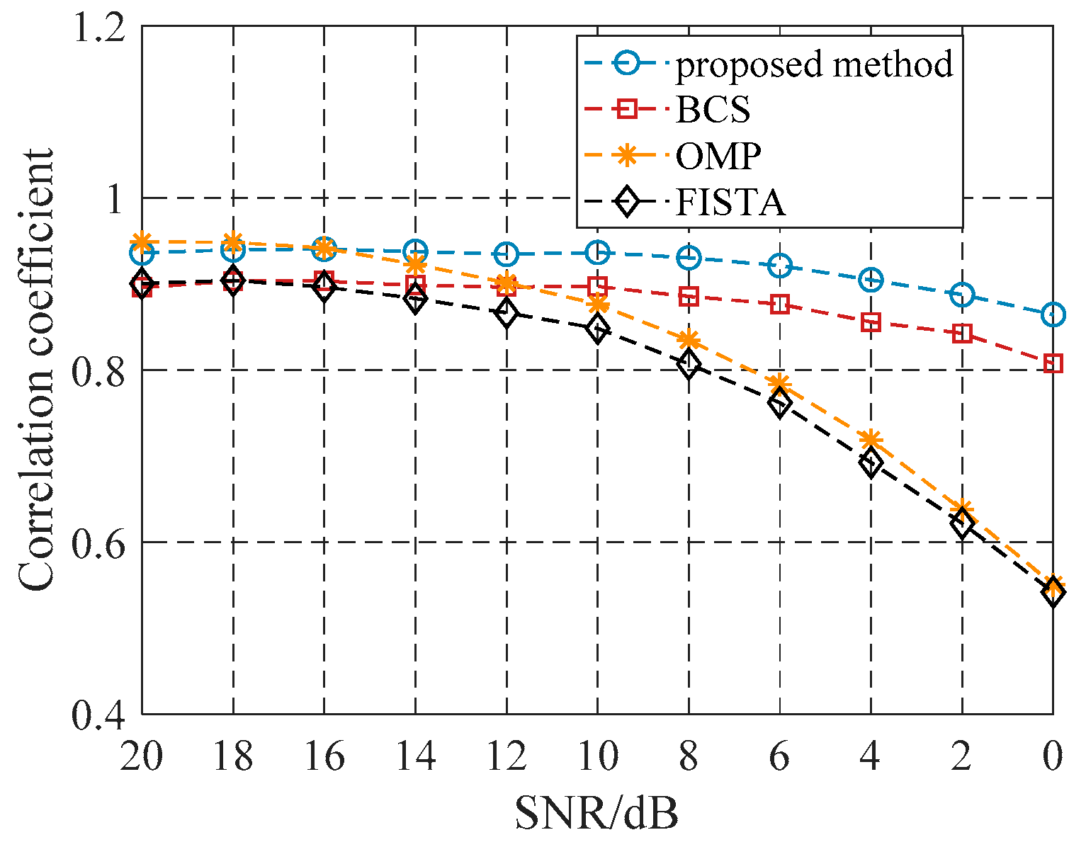
To verify the effectiveness and robustness of the proposed method, we conducted Monte Carlo tests to assess its performance in estimating target distances in different scenarios and different SNRs. We conducted 100 random experiments for each SNR, and the target positions were randomly distributed in the ranging range in each random experiment. Figure 14 and Table 3 show the average of the correlation coefficients of the four methods under different SNRs in multiple scenarios. The target-range-estimation method based on AHRC l 1 minimization effectively estimated the target-range information under a low SNR. It is worth noting that it showed high amplitude and phase-estimation accuracy. With a decrease in the SNR, the performance of the proposed method was much better than that of other reference methods, which further shows that the proposed method can estimate the target-distance information with high performance under low-SNR and small-sample conditions.
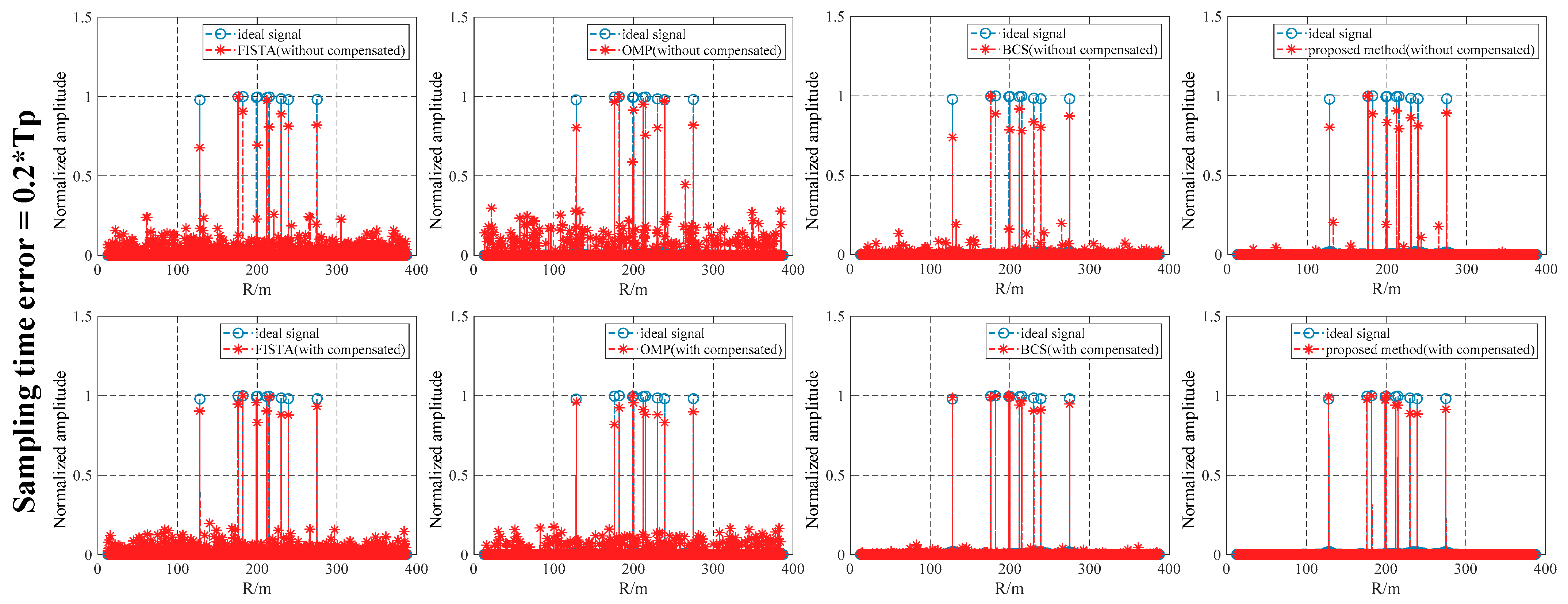
To further evaluate the performance of the proposed method, the performance of the target-range-estimation results under the SNR were compared and analyzed in combination with the sampling-time error. Figure 15, Figure 16 and Figure 17 show the distance-estimation results obtained by different methods under 10 dB SNR when the sampling-time error is 0.02 T P , 0.1 T P , and 0.2 T P , respectively. The target-range information was obtained by different algorithms without sampling-time error compensation and is shown in the first row in Figure 15, Figure 16 and Figure 17. The target-range information obtained by different algorithms with sampling-time error compensation is shown in the second row in Figure 15, Figure 16 and Figure 17. It can be clearly seen that the performance of the different algorithms with sampling-time error compensation was significantly higher than that of the algorithm without error compensation under a 10 dB SNR. The effectiveness of our proposed sampling-time error-compensation method is further illustrated. The distance estimation results of the proposed method were obviously better than those of the other reference methods, showing that it can accurately estimate the target-distance information without introducing false points.
We performed Monte Carlo tests to determine the target-distance-estimation performance in different scenarios and SNRs with sampling-time error compensation, and 100 random scene experiments were performed under each SNR. Figure 18 shows the average of the correlation coefficients of the four methods under different SNRs in multiple scenarios with the sampling-time error compensation. With the decrease in the SNR, the correlation coefficient of the OMP and FISTA algorithms decreased rapidly, and the correlation coefficient of the BCS algorithm was also lower than that of the proposed algorithm. This further shows that the proposed algorithm performed better under a low SNR with sampling-time error. The target distance and phase estimation were more accurate, and the proposed algorithm has strong noise robustness.

5. Conclusions

In this manuscript, we proposed a novel high-resolution ranging frame for laser radar with a small sample number under a low SNR utilizing the RIP-OMCS strategy and AHRC l 1 minimization. The RIP-OMCS strategy was designed to effectively reduce the amount of sampling. Aiming to cancel the sampling-time error, error estimation based on the cross-correlation function was proposed, and the ranging model was registered according to the estimated sampling-time error. High-resolution range-profile and target-range-estimation results were obtained by solving an optimization problem. The prior information about the target signal and features provides sparse constraints and AHRC for the optimization problem. AHRC takes into account the features of signals in different regions, which can better distinguish between the target and noise. The iterative solving procedure gradually corrects the AHRC l 1 minimization model to improve the accuracy of the solution at a low SNR. The experimental results show that the proposed method can effectively reduce the sampling data and estimate the target-range information at a low SNR.
This proposed method showed satisfactory performance in an environment with a large bandwidth, large ranging range, and low SNR, especially in the case of a limited sampling rate and storage space. However, it is worth noting that when the SNR was lower than 0 dB, the performance of the proposed method was poor. Therefore, future research directions can focus on laser-radar ranging methods under ultra-low SNR and ultra-low sampling conditions to improve performance.

Author Contributions

M.X. (Min Xue) created the research idea, wrote the manuscript, conducted the theoretical analyses, and verified the proposed method; M.X. (Mengdao Xing) and Y.G. were involved in improving the proposed method; J.F. and Z.W. designed the experiments; W.T. contributed to revising the manuscript; and all authors have read and agreed to the published version of the manuscript. All authors have read and agreed to the published version of the manuscript.

Funding

This research was funded in part by the National Natural Science Foundation of China under Grant 62301389, in part by the Open Fund of the Laboratory of Pinghu.

Data Availability Statement

No new data were created or analyzed in this study. Data sharing is not applicable to this article.

Conflicts of Interest

The authors declare no conflicts of interest.

References

  1. Amann, M.-C.; Bosch, T.M.; Lescure, M.; Myllylae, R.A.; Rioux, M. Laser ranging: A critical review of unusual techniques for distance measurement. Opt. Eng. 2001, 40, 10–19. [Google Scholar]
  2. Lu, Z.; Ge, C.; Wang, Z.; Jia, D.; Yang, T. Basics and developments of frequency modulation continuous wave LiDAR. Opto-Electron. Eng. 2019, 46, 190038-1–190038-14. [Google Scholar]
  3. Azadbakht, M.; Fraser, C.S.; Khoshelham, K. A Sparsity-Based Regularization Approach for Deconvolution of Full-Waveform Airborne Lidar Data. Remote Sens. 2016, 8, 648. [Google Scholar] [CrossRef]
  4. Swatantran, A.; Tang, H.; Barrett, T.; DeCola, P.; Dubayah, R. Rapid, High-Resolution Forest Structure and Terrain Mapping over Large Areas using Single Photon Lidar. Sci. Rep. 2016, 6, 28277. [Google Scholar] [CrossRef]
  5. Pfrunder, A.; Borges, P.V.K.; Romero, A.R.; Catt, G.; Elfes, A. Real-time autonomous ground vehicle navigation in heterogeneous environments using a 3D LiDAR. In Proceedings of the 2017 IEEE/RSJ International Conference on Intelligent Robots and Systems (IROS), Vancouver, BC, Canada, 24–28 September 2017; pp. 2601–2608. [Google Scholar]
  6. Wang, X.; Guo, L.; Li, Y.; Han, L.; Xu, Q.; Jing, D.; Li, L.; Xing, M. Noise-Robust Vibration Phase Compensation for Satellite ISAL Imaging by Frequency Descent Minimum Entropy Optimization. IEEE Trans. Geosci. Remote Sens. 2022, 60, 1–17. [Google Scholar] [CrossRef]
  7. Trahan, R.; Nemati, B.; Zhou, H.; Shao, M.; Hahn, I.; Schulze, W. Low-CNR inverse synthetic aperture LADAR imaging demonstration with atmospheric turbulence. Proc. SPIE 2016, 9846, 87–99. [Google Scholar]
  8. Chen, J.; Li, M.; Xing, M.; Xu, G.; Zhu, Y.; Li, R.; Li, W. Processing of airborne microwave photonic SAR raw data with inaccurate RSF. IEEE J. Miniaturization Air Space Syst. 2023, 4, 86–92. [Google Scholar] [CrossRef]
  9. Meta, A.; Hoogeboom, P.; Ligthart, L.P. Signal processing for FMCW SAR. IEEE Trans. Geosci. Remote Sens. 2007, 45, 3519–3532. [Google Scholar] [CrossRef]
  10. Pierrottet, D.; Amzajerdian, F.; Petway, L.; Barnes, B.; Lockard, G.; Rubio, M. Linear FMCW laser radar for precision range and vector velocity measurements. MRS Proc. 2008, 1076, 10760406. [Google Scholar] [CrossRef]
  11. Xi, R.; Ma, D.; Liu, X.; Wang, L.; Liu, Y. Intra-Pulse Frequency Coding Design for a High-Resolution Radar against Smart Noise Jamming. Remote Sens. 2022, 14, 5149. [Google Scholar] [CrossRef]
  12. Qian, X.; Jiang, W.; Deen, M.J. Single Photon Detectors for Automotive LiDAR Applications: State-of-the-Art and Research Challenges. IEEE J. Sel. Top. Quantum Electron. 2024, 30, 1–20. [Google Scholar] [CrossRef]
  13. Behroozpour, B.; Sandborn, A.M.; Wu, M.C.; Boser, B.E. Lidar system architectures and circuits. IEEE Commun. Mag. 2017, 55, 135–142. [Google Scholar] [CrossRef]
  14. Candan, C. A method for fine resolution frequency estimation from three DFT samples. IEEE Signal Process. Lett. 2011, 18, 351–354. [Google Scholar] [CrossRef]
  15. Aiello, M.; Cataliotti, A.; Nuccio, S. A comparison of spectrum estimation techniques for nonstationary signals in induction motor drive measurements. IEEE Trans. Instrum. Meas. 2005, 54, 2264–2271. [Google Scholar] [CrossRef]
  16. Bhutani, A.; Marahrens, S.; Gehringer, M.; Göttel, B.; Pauli, M.; Zwick, T. The role of millimeter-waves in the distance measurement accuracy of an FMCW radar sensor. Sensors 2019, 19, 3938. [Google Scholar] [CrossRef]
  17. Chen, A.; Huang, J.; Qiu, J.; Ke, Y.; Zheng, L.; Chen, X. Signal processing for a FMCW material level measurement system. In Proceedings of the 2016 IEEE 13th International Conference on Signal Processing (ICSP), Chengdu, China, 6–10 November 2016; pp. 244–247. [Google Scholar]
  18. Chen, J.; Li, M.; Yu, H.; Xing, M. Full-aperture processing of airborne microwave photonic SAR raw data. IEEE Trans. Geosci. Remote Sens. 2023, 61, 1–12. [Google Scholar] [CrossRef]
  19. Donoho, D.L. Compressed sensing. IEEE Trans. Inf. Theory 2006, 52, 1289–1306. [Google Scholar] [CrossRef]
  20. Giusti, E.; Cataldo, D.; Bacci, A.; Tomei, S.; Martorella, M. ISAR image resolution enhancement: Compressive sensing versus state-of-the-art super-resolution techniques. IEEE Trans. Aerosp. Electron. Syst. 2018, 54, 1983–1997. [Google Scholar] [CrossRef]
  21. Ender, J.H. On compressive sensing applied to radar. Signal Process. 2010, 90, 1402–1414. [Google Scholar] [CrossRef]
  22. Zhang, L.; Qiao, Z.-J.; Xing, M.-D.; Sheng, J.-L.; Guo, R.; Bao, Z. High-resolution ISAR imaging by exploiting sparse apertures. IEEE Trans. Antennas Propag. 2012, 60, 997–1008. [Google Scholar] [CrossRef]
  23. Xu, G.; Xing, M.-D.; Xia, X.-G.; Zhang, L.; Liu, Y.-Y.; Bao, Z. Sparse regularization of interferometric phase and amplitude for InSAR image formation based on Bayesian representation. IEEE Trans. Geosci. Remote Sens. 2015, 53, 2123–2136. [Google Scholar] [CrossRef]
  24. Jiang, N.; Du, H.; Ge, S.; Zhu, J.; Feng, D.; Wang, J.; Huang, X. High-Resolution Azimuth Missing Data SAR Imaging Based on Sparse Representation Autofocusing. Remote Sens. 2023, 15, 3425. [Google Scholar] [CrossRef]
  25. Huang, D.-r.; Zhang, L.; Xing, M.-D.; Xu, G.; Duan, J.; Bao, Z. Sparse aperture inverse synthetic aperture radar imaging of manoeuvring targets with compensation of migration through range cells. IET Radar Sonar Navig. 2014, 8, 1164–1176. [Google Scholar] [CrossRef]
  26. Zhang, L.; Wang, H.; Qiao, Z. Resolution enhancement for ISAR imaging via improved statistical compressive sensing. EURASIP J. Adv. Signal Process. 2016, 2016, 80. [Google Scholar] [CrossRef]
  27. Yu, H.; Lan, Y.; Yuan, Z.; Xu, J.; Lee, H. Phase unwrapping in InSAR: A review. IEEE Geosci. Remote Sens. Mag. 2019, 7, 40–58. [Google Scholar] [CrossRef]
  28. Yu, H.; Zhou, Y.; Ivey, S.S.; Lan, Y. Large-scale multibaseline phase unwrapping: Interferogram segmentation based on multibaseline envelope-sparsity theorem. IEEE Trans. Geosci. Remote Sens. 2019, 57, 9308–9322. [Google Scholar] [CrossRef]
  29. Tang, Y.; Qin, B.; Yan, Y.; Wang, L.; Xing, M. High-resolution and wide-swath imaging of the multiple-transmitter-multiple-receiver synthetic aperture ladar system. Infrared Laser Eng. 2016, 45, 0830001. [Google Scholar] [CrossRef]
  30. Xu, Z.; Qi, S.; Zhang, P. High Accuracy Multi-Antenna Ranging Algorithm and Performance Analysis for FMCW Radar. IEEE Trans. Radar Syst. 2023, 1, 657–668. [Google Scholar] [CrossRef]
  31. Li, D.; Zhou, K.; Cui, A.; Qiao, M.; Wu, S.; Wang, Y.; Yao, Y.; Wu, J.; Gao, J. Multi-Channel Inverse Synthetic Aperture Ladar Imaging Detection Technology and Experimental Research. Laser Optoelectron. Prog. 2021, 58, 342–353. [Google Scholar]
  32. Engels, F.; Heidenreich, P.; Wintermantel, M.; Stäcker, L.; Kadi, M.A.; Zoubir, A.M. Automotive radar signal processing: Research directions and practical challenges. IEEE J. Sel. Top. Signal Process. 2021, 15, 865–878. [Google Scholar] [CrossRef]
  33. Li, Y.; Wang, T.; Huo, T.; Nie, L. A Study on the Range Equation Modeling for Multichannel Medium-Earth-Orbit SAR-GMTI Systems. Remote Sens. 2021, 13, 2734. [Google Scholar] [CrossRef]
  34. Guo, L.; Xu, Q.; Li, X.; Zeng, X.; Tang, Y.; Xing, M. Multi-channel scan mode and imaging algorithm for synthetic aperture ladar. Optik 2021, 155, 225–232. [Google Scholar] [CrossRef]
  35. Xu, G.; Liu, Y.; Xing, M. Multi-channel synthetic aperture radar imaging of ground moving targets using compressive sensing. IEEE Access 2018, 6, 66134–66142. [Google Scholar] [CrossRef]
  36. Yao, Z.; Mauldin, T.; Hefferman, G.; Wei, T. Digitally integrated self-trained predistortion curve finder for passive sweep linearization of semiconductor lasers. IEEE J. Sel. Top. Quantum Electron. 2019, 25, 1–5. [Google Scholar] [CrossRef]
  37. Xu, X.; Chen, Y.; Zhu, K.; Yang, J.; Tan, Z.; Luo, M. Research on FPGA pulse laser ranging method based on deep learning. IEEE Trans. Instrum. Meas. 2021, 70, 1–11. [Google Scholar] [CrossRef]
  38. Yuan, S.; Yan, X.; Xu, J.; Zhu, W.; Qin, H. Cognitive Imaging Lidar Based on Deep Learning. Acta Photonica Sin. 2021, 50, 1011002. [Google Scholar]
  39. Liu, B.; Liu, J. A Method of the Realization of High Accuracy in FMCW Ranging System. J. Instrum. 2001, 15, 41–45. [Google Scholar]
  40. Li, Z.; Zhang, R.; Yang, J.; Xiong, J. Improving Range Precision of LFMCW Radar with Frequency Domain Up-Sampling-Interpolating Method. Telecommun. Eng. 2005, 45, 77–80. [Google Scholar]
  41. Vasilyev, A.; Satyan, N.; Xu, S.; Rakuljic, G.; Yariv, A. Multiple source frequency-modulated continuous-wave optical reflectometry: Theory and experiment. App. Opt. 2010, 49, 1932–1937. [Google Scholar] [CrossRef]
  42. Scherr, S.; Ayhan, S.; Fischbach, B.; Bhutani, A.; Pauli, M.; Zwick, T. An efficient frequency and phase estimation algorithm with CRB performance for FMCW radar applications. IEEE Trans. Instrum. Meas. 2015, 64, 1868–1875. [Google Scholar] [CrossRef]
  43. Xu, Z.; Qi, S.; Zhang, P. A coherent CZT-based algorithm for high-accuracy ranging with FMCW radar. IEEE Trans. Instrum. Meas. 2023, 72, 1–11. [Google Scholar] [CrossRef]
  44. Zhang, T.; Qu, X.; Zhang, F. The Slight Vibrations Compensation of FMCW Ranging Method Based on Three Light Paths Structure. Spectrosc. Spect. Anal. 2020, 40, 1007–1011. [Google Scholar]
  45. He, J.; Zhang, Q.; Yang, X.; Luo, Y.; Ji, N. Sampling Technology of ISAIL. Acta Photonica Sin. 2010, 39, 1272–1277. [Google Scholar]
  46. Zang, B.; Guo, R.; Zhang, L.; Tang, Y.; Xing, M. A Phase Adjustment Algorithm for ISAIL Based on Sparsity. Acta Electonica Sin. 2011, 39, 1272–1277. [Google Scholar]
  47. Tian, H.; Mao, H.; Liu, Z.; Zeng, Z. Airborne ladar sparse imaging on targets with micro-motions based on inverse synthetic aperture technique. Infrared Laser Eng. 2020, 49, 20200190. [Google Scholar]
  48. Wu, S.; Ding, L.; Li, P.; Chen, L.; Zhu, Y. Millimeter-Wave SAR Sparse Imaging With 2-D Spatially Pseudorandom Spiral-Sampling Pattern. IEEE Trans. Microw. Theory Tech. 2020, 68, 4672–4683. [Google Scholar] [CrossRef]
  49. Wang, L.; Ai, Z.; Shi, J.; Wang, J.; Zhang, X.; Yang, J. Low Computational Complexity SAR Imaging Algorithm for Ship Monitoring via 2-D Band-Limited Sparse Fourier Transform. IEEE Sens. J. 2024, 24, 13326–13342. [Google Scholar] [CrossRef]
  50. Fan, J.; Wu, Y.; Wang, F.; Zhang, P.; Li, M. New Point Matching Algorithm Using Sparse Representation of Image Patch Feature for SAR Image Registration. IEEE Trans. Geosci. Remote Sens. 2017, 55, 1498–1510. [Google Scholar] [CrossRef]
  51. Pu, W.; Bao, Y. RPCA-AENet: Clutter Suppression and Simultaneous Stationary Scene and Moving Targets Imaging in the Presence of Motion Errors. IEEE Trans. Neural Netw. Learn. Syst. 2024, 35, 2339–2352. [Google Scholar] [CrossRef]
  52. Romero, D.; Ariananda, D.D.; Tian, Z.; Leus, G. Compressive covariance censing: Structure-based compressive sensing beyond sparsity. IEEE Signal Process. Mag. 2016, 33, 78–93. [Google Scholar] [CrossRef]
  53. Candes, E.J. The restricted isometry property and its implications for compressed sensing. Comptes Rendus Math. 2008, 346, 589–592. [Google Scholar] [CrossRef]
  54. Tsaig, Y.; Donoho, D.L. Extensions of compressed sensing. Signal Process. 2006, 86, 549–571. [Google Scholar] [CrossRef]
  55. Wipf, D.; Nagarajan, S. Solving sparse linear inverse problems: Analysis of reweighted L1 and L2 methods. In Proceedings of the Signal Processing with Adaptive Sparse Structured Representations (SPARS), Saint-Malo, France, 6–9 April 2009; pp. 1–7. [Google Scholar]
  56. Huang, Y.; Liao, G.; Zhang, L.; Xiang, Y.; Li, J.; Nehorai, A. Efficient narrowband RFI mitigation algorithms for SAR systems with reweighted tensor structures. IEEE Trans. Geosci. Remote Sens. 2019, 57, 9396–9409. [Google Scholar] [CrossRef]
  57. Xu, G.; Zhang, B.; Yu, H.; Chen, J.; Xing, M.; Hong, W. Sparse synthetic aperture radar imaging from compressed sensing and machine learning: Theories applications and trends. IEEE Geosci. Remote Sens. Mag. 2022, 10, 32–69. [Google Scholar] [CrossRef]
Figure 1. Typical laser-radar ranging system.
Remotesensing 16 01647 g001
Figure 2. Principle diagram of laser-radar ranging.
Remotesensing 16 01647 g002
Figure 3. Multi-channel coprime low-sampling scheme.
Remotesensing 16 01647 g003
Figure 4. Flowchart of the proposed method.
Remotesensing 16 01647 g004
Figure 5. Asynchronous sampling-time error diagram.
Remotesensing 16 01647 g005
Figure 6. Sampling-time error-estimation diagram.
Remotesensing 16 01647 g006
Figure 7. Flowchart of the AHRC.
Remotesensing 16 01647 g007
Figure 8. Flowchart of the range-estimation method based on AHRC l 1 minimization.
Remotesensing 16 01647 g008
Figure 9. Performance comparison of different coprime combinations. (a) Maximum and minimum eigenvalues of different coprime combinations; (b) RICs of different coprime combinations.
Remotesensing 16 01647 g009
Figure 10. Performance comparison of optimal coprime combinations. (a) Range profile of Nyquist sampling. (b) Range profile of ADC1. (c) Range profile of ADC2. (d) Range profile of ADC3. (e) Range profile of the proposed method. (f) Target phase difference. (g) Two-dimensional figure of target range phase. (h) CORR under 10 scenes.
Remotesensing 16 01647 g010
Figure 11. Comparison of the results before and after the sampling-time error compensation. (a) With compensation. (b) Without compensation. (c) Two-dimensional figure of target range phase. (d) CORR under 10 sampling-time error scenarios.
Remotesensing 16 01647 g011
Figure 12. Average of the correlation coefficient under different sampling-time error conditions. (a) Correlation coefficient under Channel 2 with sampling-time error of 0 0.2 T P . (b) Correlation coefficient under Channel 3 with sampling-time error of 0 0.2 T P . (c) Correlation coefficient under Channels 2 and 3 in 0 0.2 T P sampling-time error conditions.
Remotesensing 16 01647 g012
Figure 13. Target-range-estimation result of different algorithms under different SNRs.
Remotesensing 16 01647 g013
Figure 14. Average of the correlation coefficients of four methods under different SNRs in multiple scenarios.
Remotesensing 16 01647 g014
Figure 15. Target-range-estimation result of different algorithms under 10 dB SNR when the sampling-time error is 0.02 T P .
Remotesensing 16 01647 g015
Figure 16. Target-range-estimation result of different algorithms under 10 dB SNR when the sampling-time error is 0.1 T P .
Remotesensing 16 01647 g016
Figure 17. Target-range-estimation result of different algorithms under 10 dB SNR when the sampling-time error is 0.2 T P .
Remotesensing 16 01647 g017
Figure 18. Average of the correlation coefficients of the four methods under different SNRs in multiple scenarios with the sampling-time error compensation. (a) Sampling-time error is 0.02 T P . (b) Sampling-time error is 0.1 T P . (c) Sampling-time error is 0.2 T P .
Remotesensing 16 01647 g018
Table 1. Parameters used in the simulation.
ParameterValue ParameterValue
Wavelength1.55 μmR0200 m
Pulse width28 μs Ranging   range   Δ R 300 m
Bandwidth1 GHzFs89.3 MHz
Table 2. Multi-channel coprime low-sampling combination.
ParameterADC 1ADC 2ADC 3ADC 4Downsampling Rate
Coprime Combination 1Fs/11Fs/1316.78%
Coprime Combination 2Fs/17Fs/18Fs/1916.7%
Coprime Combination 3Fs/13Fs/29Fs/37Fs/4016.34%
Table 3. Average of the correlation coefficients under different SNRs in multiple scenarios.
20 dB18 dB16 dB14 dB12 dB10 dB8 dB6 dB4 dB2 dB0 dB
Proposed method94%94%94%94%93%93%93%92%90%89%86%
BCS90%90%90%90%90%90%89%88%86%84%80%
OMP95%95%94%92%90%88%83%78%72%64%55%
FISTA90%90%90%88%87%85%81%76%69%62%54%
Disclaimer/Publisher’s Note: The statements, opinions and data contained in all publications are solely those of the individual author(s) and contributor(s) and not of MDPI and/or the editor(s). MDPI and/or the editor(s) disclaim responsibility for any injury to people or property resulting from any ideas, methods, instructions or products referred to in the content.