


Modeling Canopy Height of Forest–Savanna Mosaics in Togo Using ICESat-2 and GEDI Spaceborne LiDAR and Multisource Satellite Data


Abstract
1. Introduction
2. Materials and Methods
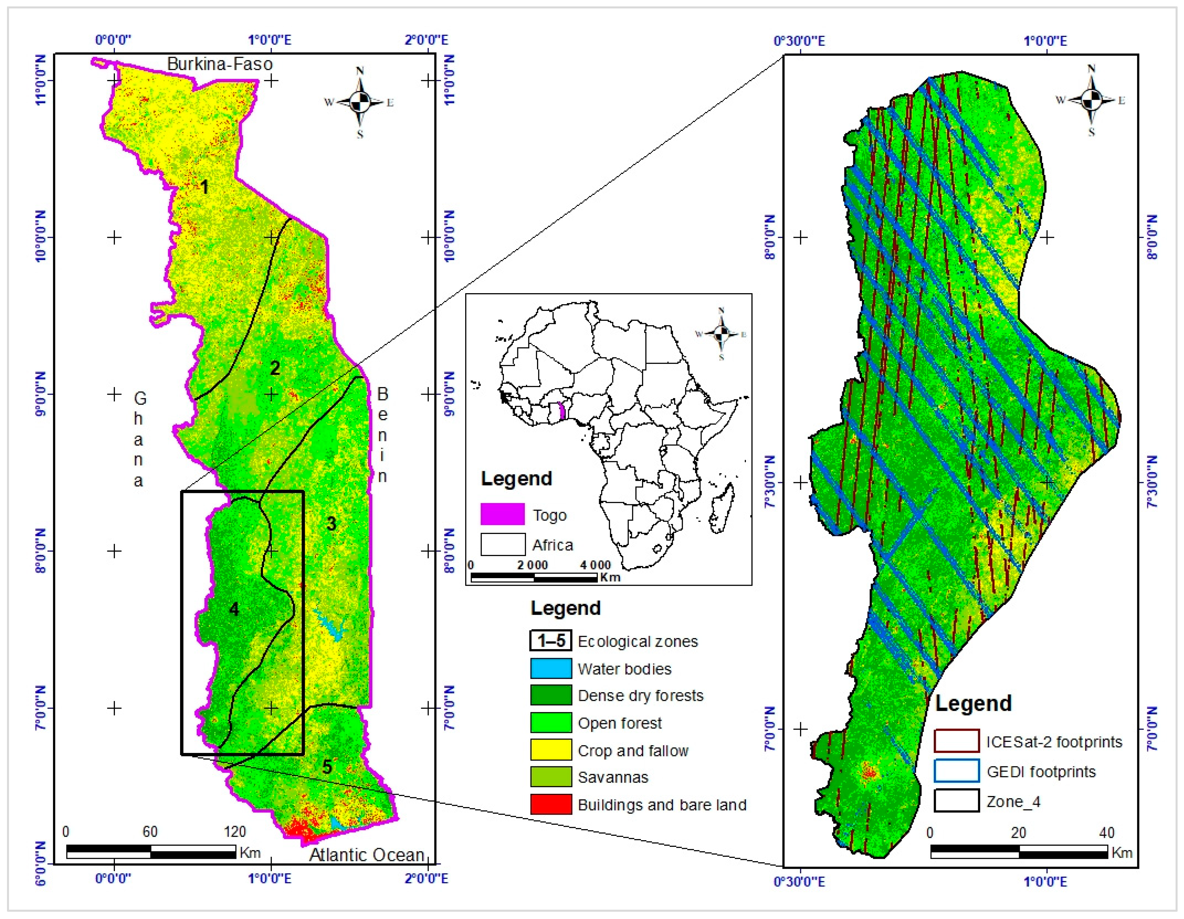
2.1. Study Area
2.2. Data Collection and Preprocessing
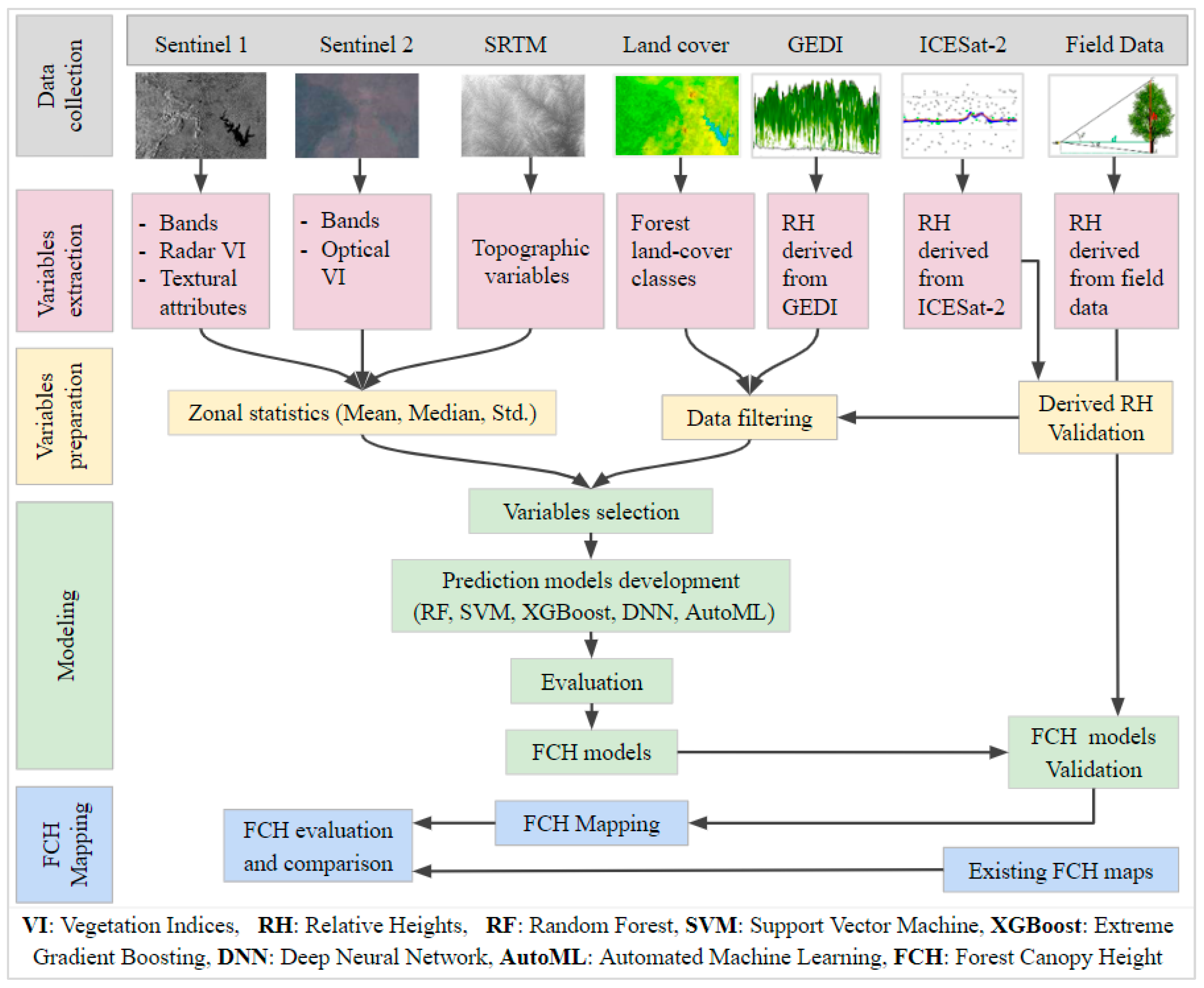
2.3. Methods
2.3.1. Feature Extraction
2.3.2. Dataset Preparation
- Validation of satellite LiDAR data
- Data filtering
- Calculation of zonal statistics
2.3.3. Modeling
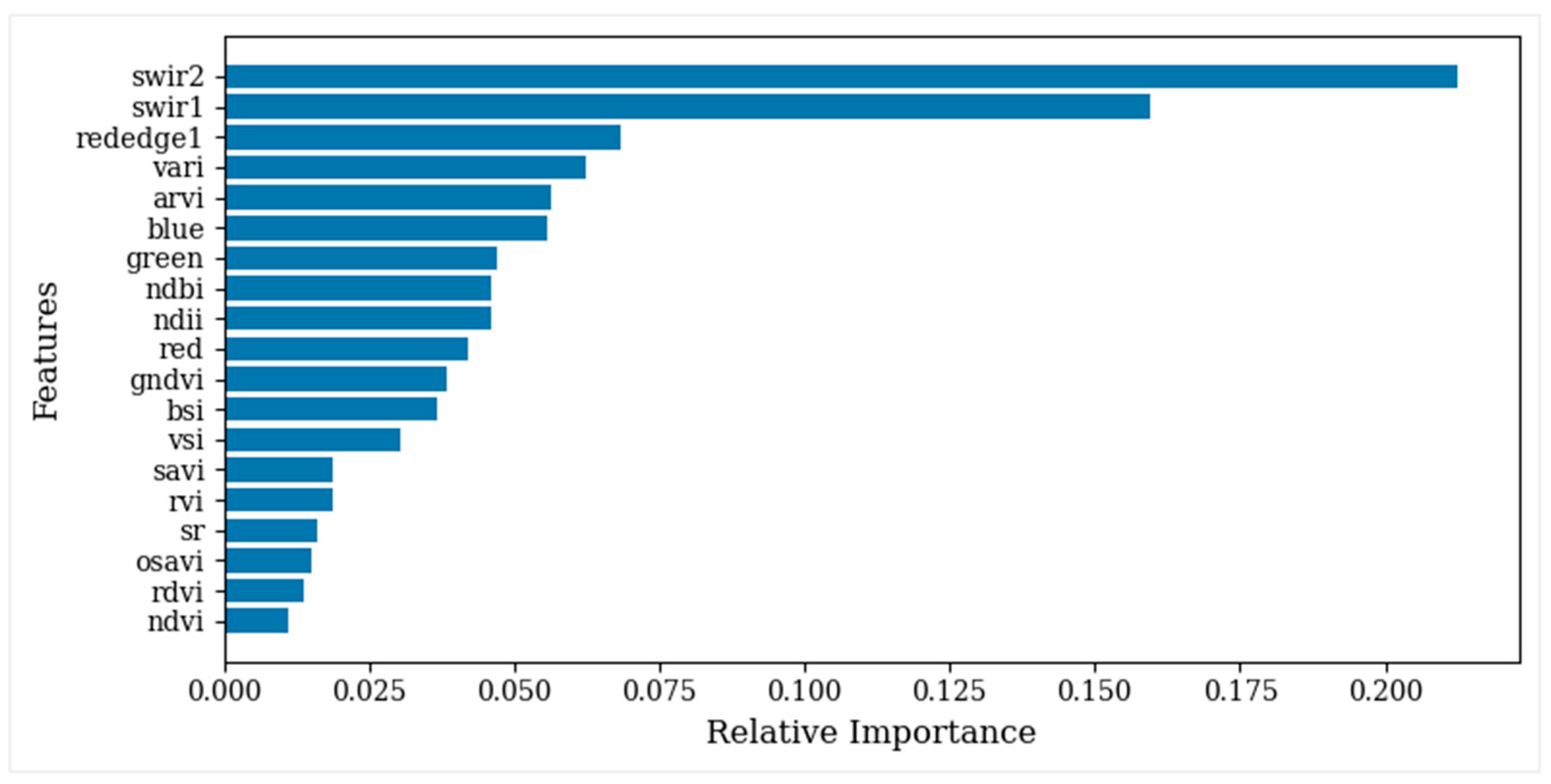
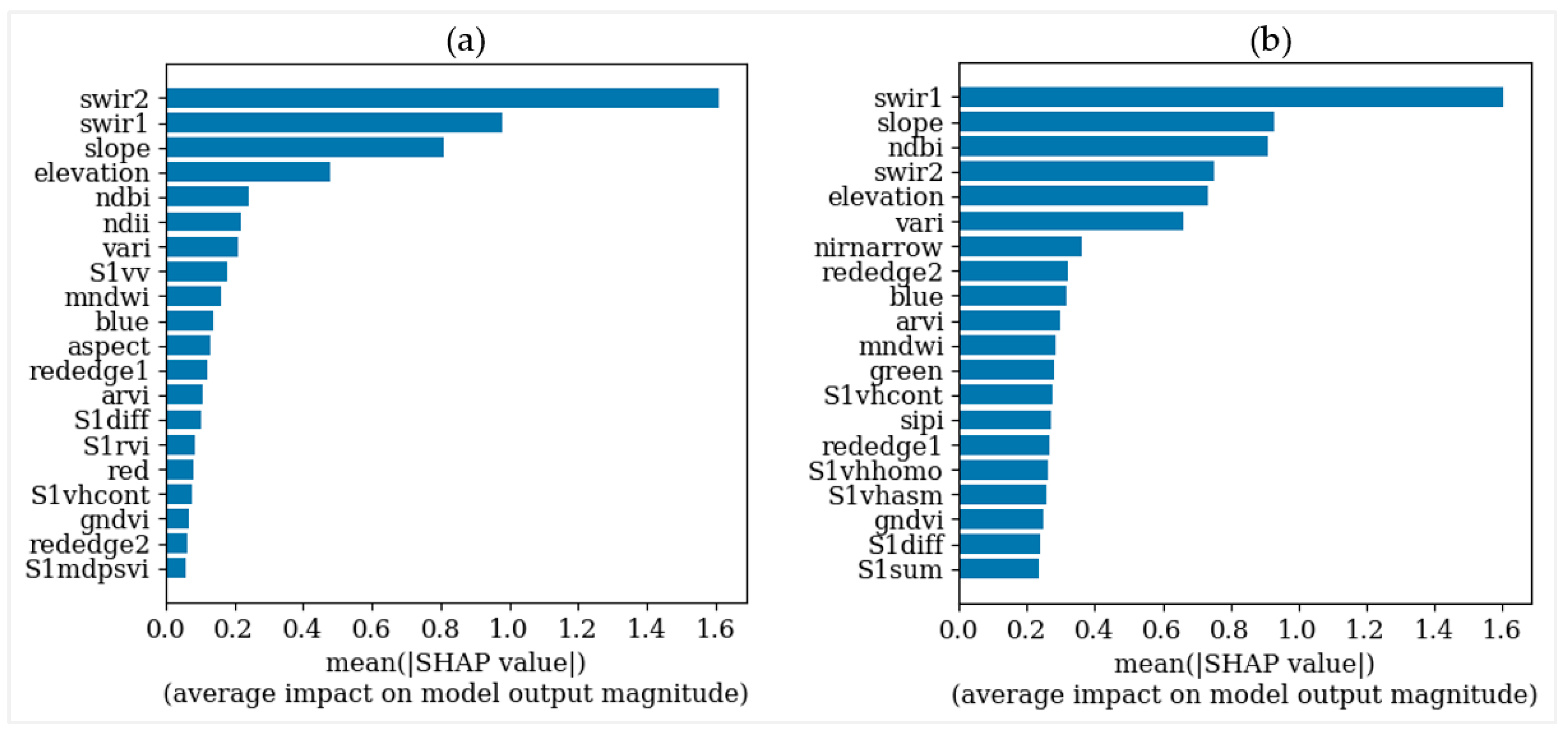
- Features selection
- Development of prediction models
- Performance evaluation of the developed models
2.4. Forest Height Mapping and Comparison with Existing Products
3. Results
3.1. Validation of the Reference Data
3.2. Selection and Combination of Multisource Variables
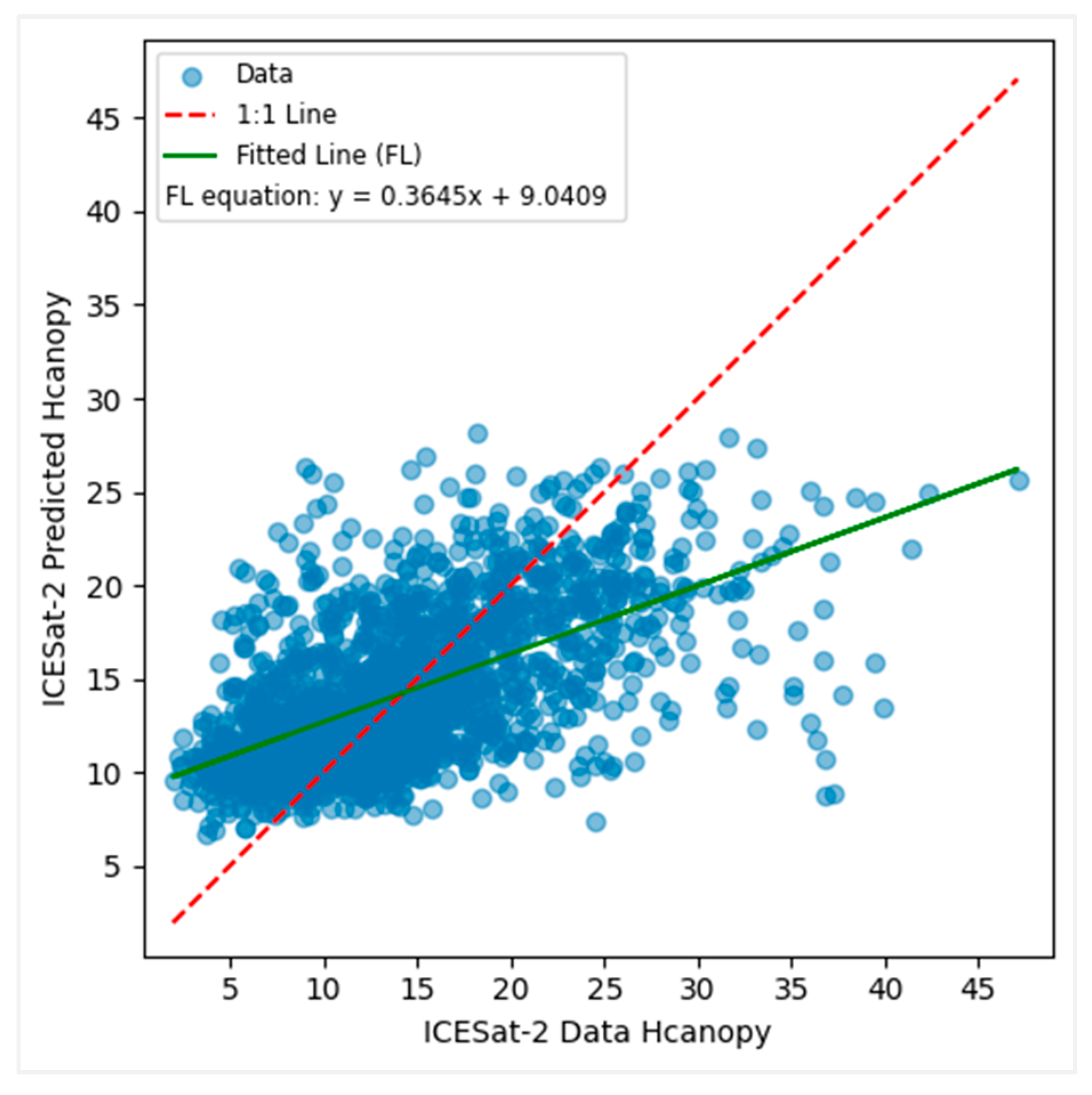
3.3. Modeling Canopy Height Using ICESat-2 Data
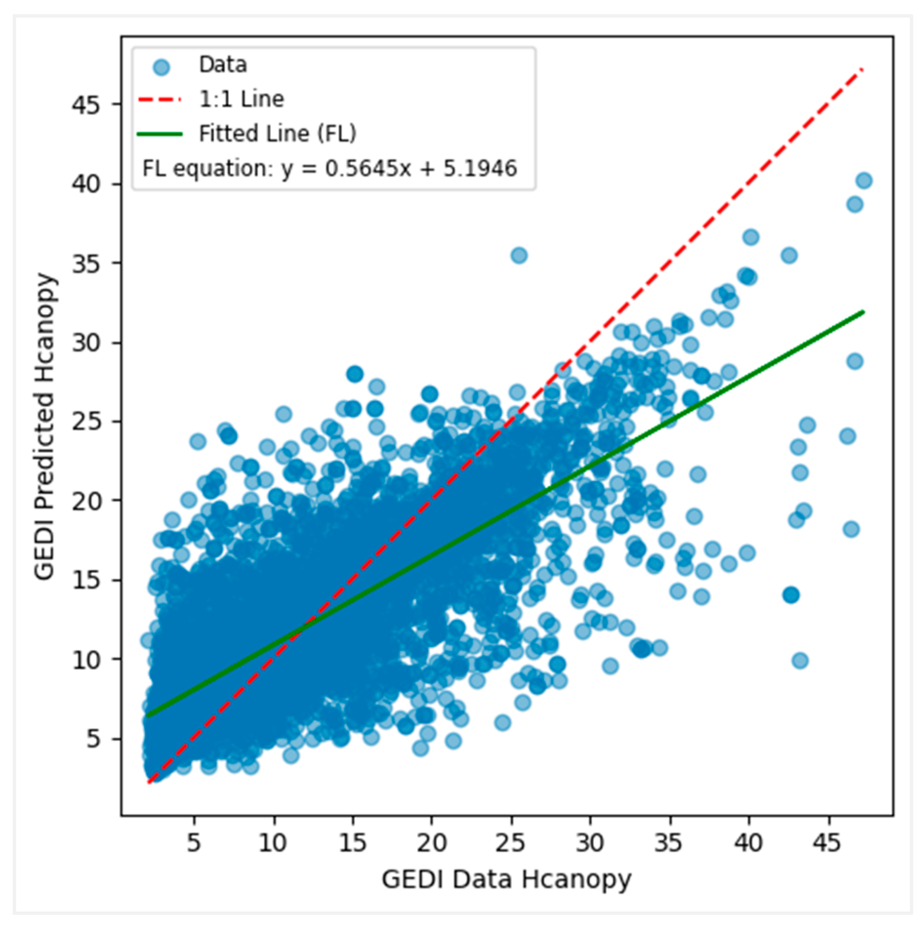
3.4. Modeling Canopy Height from GEDI Data
3.5. Forest Canopy Height Mapping from Developed Models
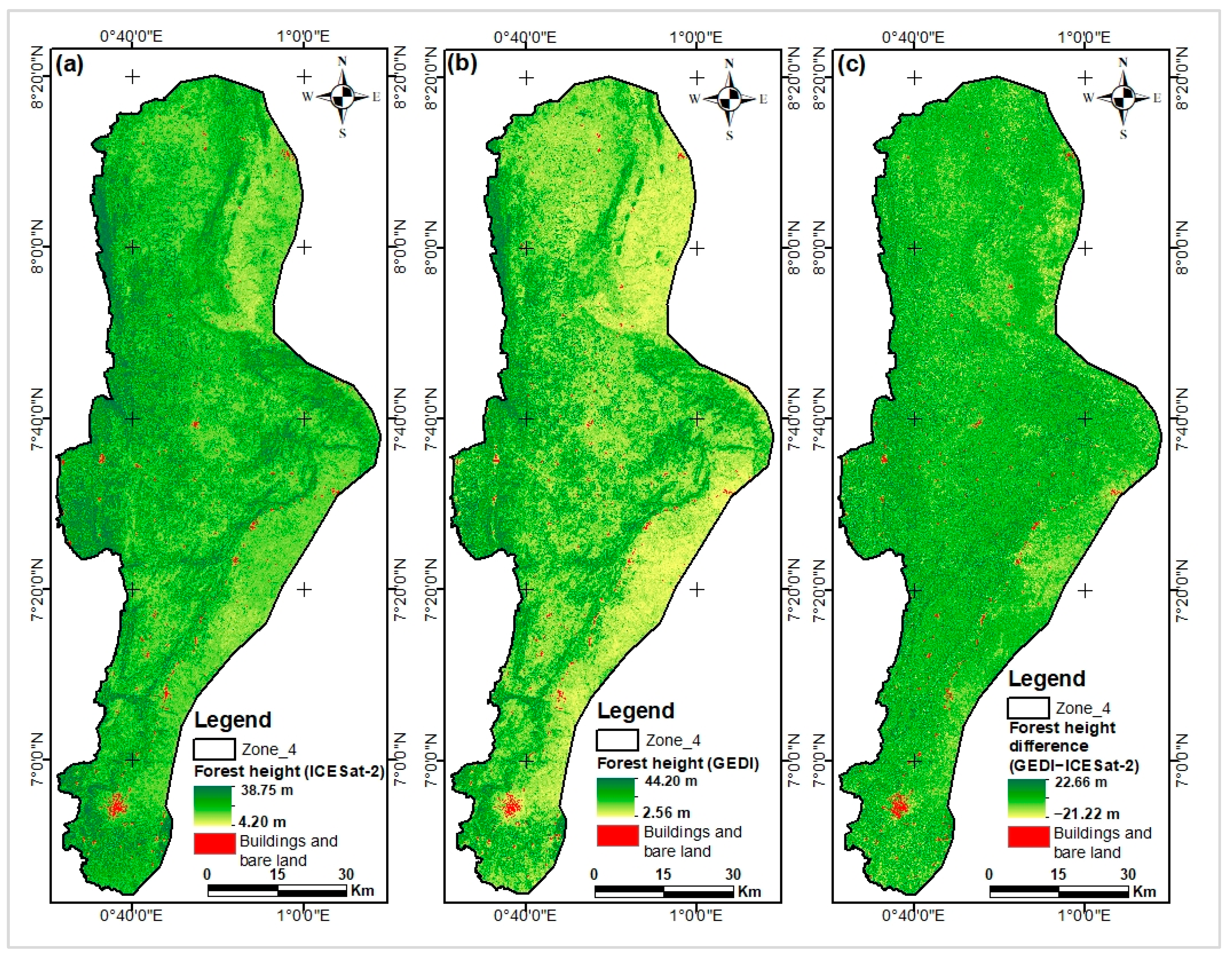
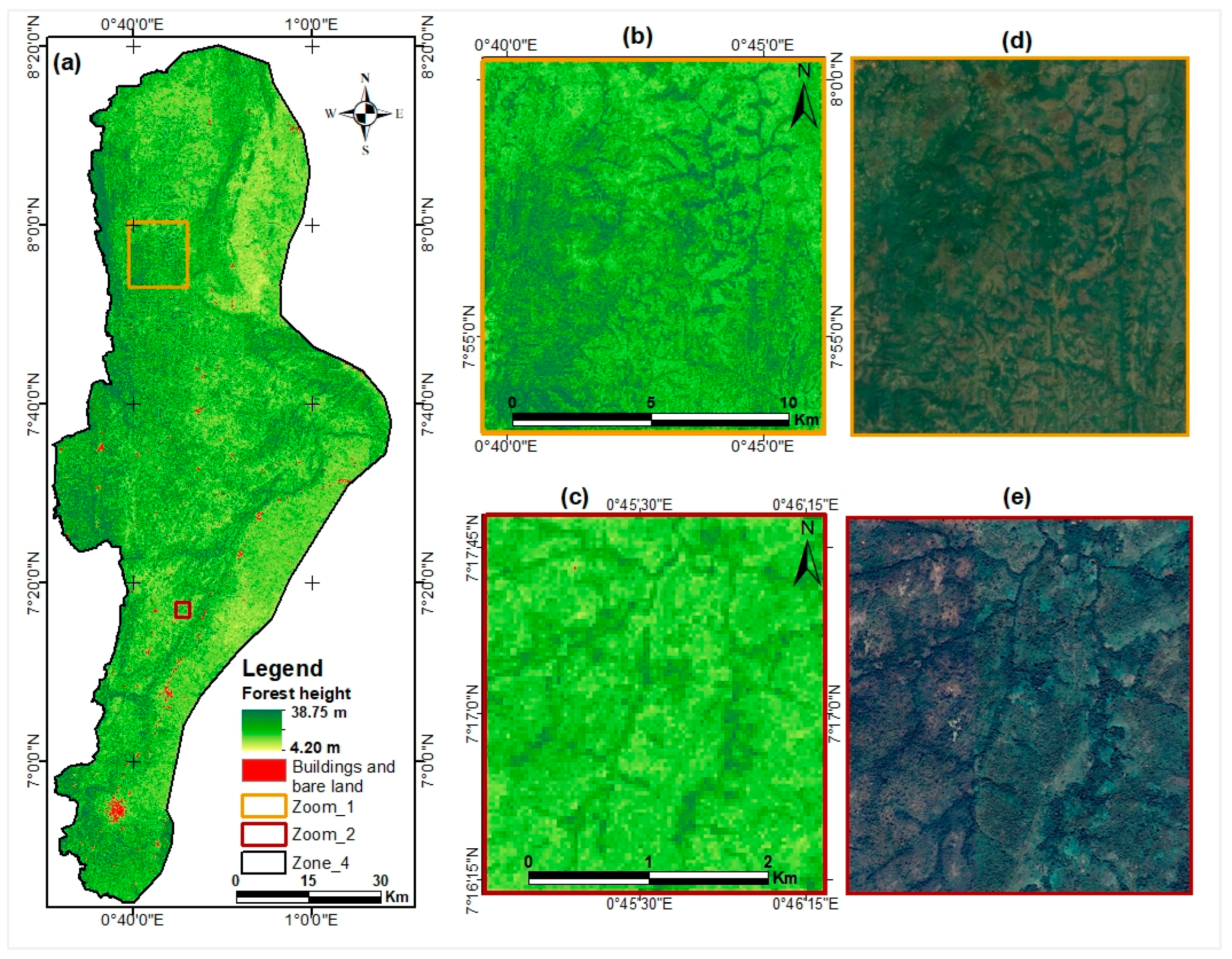
3.5.1. Forest Canopy Height Map Created from the ICESat-2 Based Model
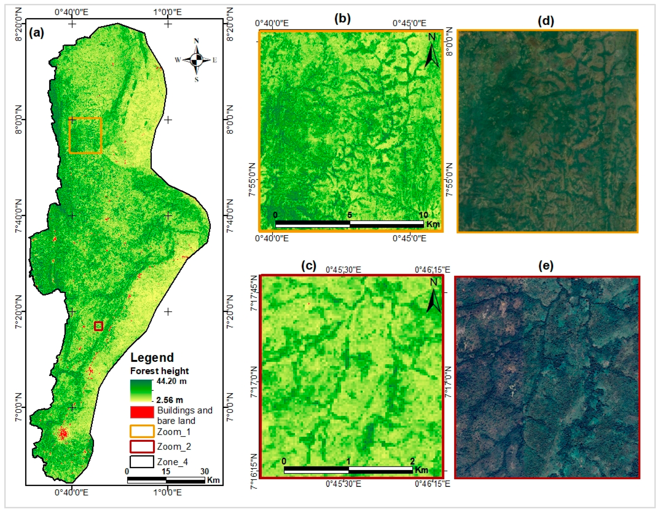
3.5.2. Forest Canopy Height Map from GEDI-Based Model
3.6. Comparative Analysis of Developed Models with Existing Products
4. Discussion
5. Conclusions
Author Contributions
Funding
Data Availability Statement
Acknowledgments
Conflicts of Interest
Appendix A
Appendix B

| Covariates | Description | Covariates | Description |
|---|---|---|---|
| S1vv | Vertical transmit, Vertical receive polarization | green | Sentinel2 B3 |
| S1vh | Vertical transmit, Horizontal receive polarization | red | Sentinel2 B4 |
| S1diff | Bands difference between VV and VH | rededge1 | Sentinel2 B5 |
| S1mdpsvi | Modified Dual Polarimetric Sar Vegetation Index | rededge2 | Sentinel2 B6 |
| S1npdi | Normalized Polarization Difference Index | rededge3 | Sentinel2 B7 |
| S1prod | Bands product between VV and VH | nir | Sentinel2 B8 |
| S1rept | Bands report between VV and VH | nirnarrow | Sentinel2 B8A |
| S1rvi | Ratio Vegetation Index | swir1 | Sentinel2 B11 |
| S1sum | Bands sum between VV and VH | swir2 | Sentinel2 B12 |
| S1vhasm | VH GLCM Angular Second Moment | arvi | Atmospherically Resistant Vegetation Index |
| S1vhcont | VH GLCM Contrast | bsi | Bare Soil Index |
| S1vhcorr | VH GLCM Correlation | evi | Enhanced Vegetation Index |
| S1vhdiss | VH GLCM Dissimilarity | gndvi | Green Normalized Difference Vegetation Index |
| S1vhener | VH GLCM Energy | mndwi | Modified Normalized Difference Water Index |
| S1vhent | VH GLCM Entropy | msavi | Modified Soil Adjusted Vegetation Index |
| S1vhhomo | VH GLCM Inverse Difference Moment | mtvi | Modified Triangular Vegetation Index |
| S1vhmax | VH GLCM Maximum | ndbi | Normalized Difference Built-up Index |
| S1vhmean | VH GLCM Mean | ndii | Normalized Difference Infrared Index |
| S1vhvar | VH GLCM Variance | ndvi | Normalized Difference Vegetation Index |
| S1vvasm | VV GLCM Angular Second Moment | osavi | Optimized Soil Adjusted Vegetation Index |
| S1vvcont | VV GLCM Contrast | rdvi | Renormalized Difference Vegetation Index |
| S1vvcorr | VV GLCM Correlation | rvi | Ratio Vegetation Index |
| S1vvdiss | VV GLCM Dissimilarity | savi | Soil Adjusted Vegetation Index |
| S1vvener | VV GLCM Energy | sipi | Structure Insensitive Pigment Index |
| S1vvent | VV GLCM Entropy | sr | Simple Ratio |
| S1vvhomo | VV GLCM Inverse Difference Moment | vari | Visible Atmospherically Resistant Index |
| S1vvmax | VV GLCM Maximum | vsi | Vegetation Structure Index |
| S1vvmean | VV GLCM Mean | aspect | SRTM aspect |
| S1vvvar | VV GLCM Variance | elevation | SRTM elevation |
| blue | Sentinel2 B2 | slope | SRTM slope |
Appendix C
| No. | Feature Abbrev. | Description | Native Band/Formula | References |
|---|---|---|---|---|
| 1 | S1vv | Vertical transmit—vertical channel backscattering coefficients, dB | VV | [106] |
| 2 | S1vh | Vertical transmit—horizontal channel backscattering coefficients, dB | VH | [106] |
| 3 | S1diff | Bands difference between VV and VH | [107] | |
| 4 | S1mdpsvi | Modified Dual Polarimetric Sar Vegetation Index | [108] | |
| 5 | S1npdi | Normalized Polarization Difference Index | [109] | |
| 6 | S1prod | Bands product between VV and VH | [107] | |
| 7 | S1rept | Bands report between VV and VH | [16] | |
| 8 | S1rvi | Ratio Vegetation Index | 4 × VH/(VV + VH) | [107] |
| 9 | S1sum | Bands sum between VV and VH | [110] | |
| 10 | S1vhasm | VH GLCM * Angular Second Moment | [111] | |
| 11 | S1vhcont | VH GLCM Contrast | [111] | |
| 12 | S1vhcorr | VH GLCM Correlation | [111] | |
| 13 | S1vhdiss | VH GLCM Dissimilarity | [111] | |
| 14 | S1vhener | VH GLCM Energy | [111] | |
| 15 | S1vhent | VH GLCM Entropy | [111] | |
| 16 | S1vhhomo | VH GLCM Homogeneity | [111] | |
| 17 | S1vhmax | VH GLCM Maximum | [111] | |
| 18 | S1vhmean | VH GLCM Mean | [111] | |
| 19 | S1vhvar | VH GLCM Variance | [111] | |
| 20 | S1vvasm | VV GLCM Angular Second Moment | [111] | |
| 21 | S1vvcont | VV GLCM Contrast | [111] | |
| 22 | S1vvcorr | VV GLCM Correlation | [111] | |
| 23 | S1vvdiss | VV GLCM Dissimilarity | [111] | |
| 24 | S1vvener | VV GLCM Energy | [111] | |
| 25 | S1vvent | VV GLCM Entropy | [111] | |
| 26 | S1vvhomo | VV GLCM Homogeneity | [111] | |
| 27 | S1vvmax | VV GLCM Maximum | [111] | |
| 28 | S1vvmean | VV GLCM Mean | [111] | |
| 29 | S1vvvar | VV GLCM Variance | [111] | |
| 30 | blue | Blue band | B2 | [112] |
| 31 | green | Green band | B3 | [112] |
| 32 | red | Red band | B4 | [112] |
| 33 | rededge1 | Red edge1 band | B5 | [112] |
| 34 | rededge2 | Red edge2 band | B6 | [112] |
| 35 | rededge3 | Red edge3 band | B7 | [112] |
| 36 | nir | Near-infrared (NIR) band | B8 | [112] |
| 37 | nirnarrow | Near-infrared narrow (NIR–narrow) band | B8A | [112] |
| 38 | wir1 | Short-wave infrared (SWIR1) band | B11 | [112] |
| 39 | swir2 | Short-wave infrared (SWIR 2) band | B12 | [112] |
| 40 | arvi | Atmospherically Resistant Vegetation Index | NIR − (2 × Red − Blue)/NIR + (2 × Red − Blue) | [113] |
| 41 | bsi | Bare Soil Index | [114] | |
| 42 | evi | Enhanced Vegetation Index | 2.5 × (NIR − Red)/(NIR + 6Red − 7.5 × Blue + 1) | [113] |
| 43 | gndvi | Green Normalized Difference Vegetation Index | (NIR − Green)/(NIR + Green) | [16] |
| 44 | mndwi | Modified Normalized Difference Water Index | (Green − SWIR)/(Green + SWIR) | [115] |
| 45 | msavi | Modified Soil Adjusted Vegetation Index | [116] | |
| 46 | mtvi | Modified Triangular Vegetation Index | 1.2 × [1.2(NIR − Green) − 2.5 × (Red − Green)] | [67] |
| 47 | ndbi | Normalized Difference Built-up Index | [117] | |
| 48 | ndii | Normalized Difference Infrared Index | [118] | |
| 49 | ndvi | Normalized Difference Vegetation Index | (NIR − Red)/(NIR + Red) | [113] |
| 50 | osavi | Optimized Soil Adjusted Vegetation Index | [119] | |
| 51 | rdvi | Renormalized Difference Vegetation Index | [120] | |
| 52 | rvi | Ratio Vegetation Index | (Red/NIR) | [121] |
| 53 | savi | Soil Adjusted Vegetation Index | 1.5 × (NIR − Red)/(NIR + Red + 0.5) | [122] |
| 54 | sipi | Structure Insensitive Pigment Index | (NIR − Blue)/(NIR − Red) | [67] |
| 55 | sr | Simple Ratio | (NIR/Red) | [123] |
| 56 | vari | Visible Atmospherically Resistant Index | (Green − Red)/(Green + Red − Blue) | [124] |
| 57 | vsi | Vegetation Structure Index | NDVI/(1 − NIR) | [125] |
| 58 | aspect | Aspect | [126] | |
| 59 | elevation | Elevation | [126] | |
| 60 | slope | Slope | [126] |
Appendix D
Appendix E
- Random Forest
- Support Vector Machine
- Extreme Gradient Boosting
- Deep Neural Network
Appendix F
Appendix G
Appendix H. Difference Between Canopy Height Maps by Subtraction
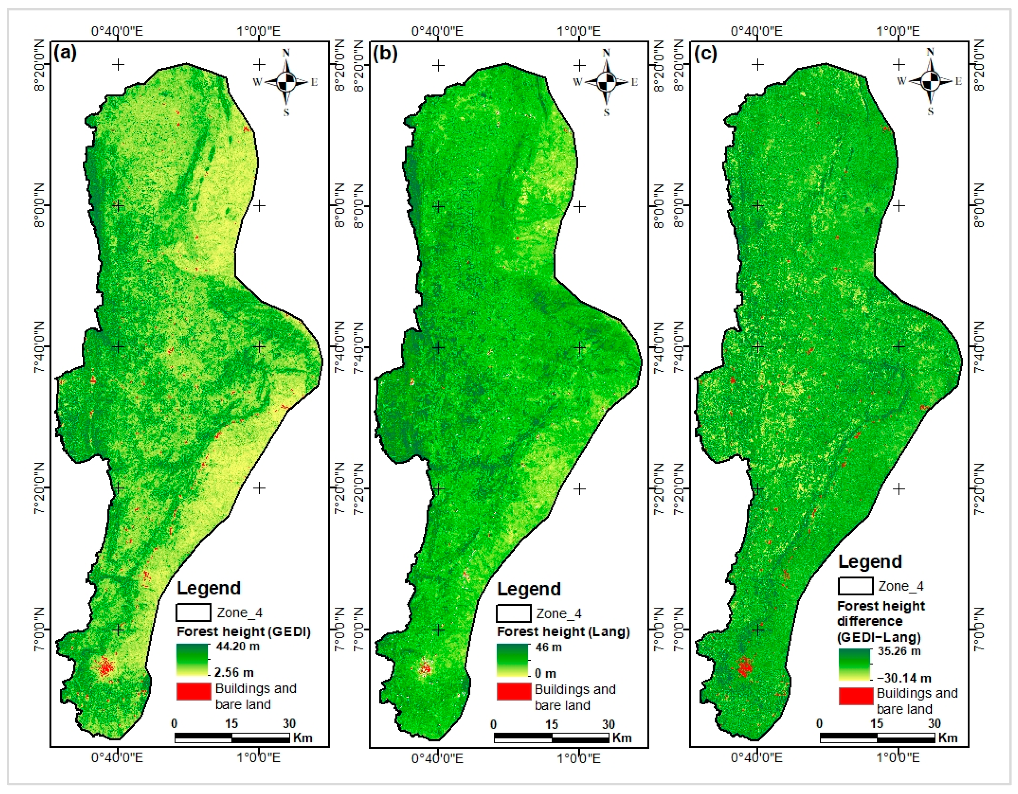

Appendix I. Comparing Our Models Maps with Lang and Potapov Maps

References
- Van Houtan, K.S.; Tanaka, K.R.; Gagné, T.O.; Becker, S.L. The Geographic Disparity of Historical Greenhouse Emissions and Projected Climate Change. Sci. Adv. 2021, 7, eabe4342. [Google Scholar] [CrossRef] [PubMed]
- Xu, X.; Huang, A.; Belle, E.; De Frenne, P.; Jia, G. Protected Areas Provide Thermal Buffer against Climate Change. Sci. Adv. 2022, 8, eabo0119. [Google Scholar] [CrossRef]
- Moore, J.W.; Schindler, D.E. Getting Ahead of Climate Change for Ecological Adaptation and Resilience. Science 2022, 376, 1421–1426. [Google Scholar] [CrossRef] [PubMed]
- Babiker, M.; Berndes, G.; Blok, K.; Cohen, B.; Cowie, A.; Geden, O.; Ginzburg, V.; Leip, A.; Smith, P.; Sugiyama, M.; et al. Cross-Sectoral Perspectives (Chapter 12). In IPCC, 2022: Climate Change 2022: Mitigation of Climate Change. Contribution of Working Group III to the Sixth Assessment Report of the Intergovernmental Panel on Climate Change; Shukla, A.R., Skea, J., Slade, R., Al Khourdajie, A., van Diemen, R., McCollum, D., Pathak, M., Some, S., Vyas, P., Fradera, R., et al., Eds.; Cambridge University Press: Cambridge, UK; New York, NY, USA, 2022; pp. 1245–1354. ISBN 978-1-009-15792-6. [Google Scholar]
- Fischer, H.W.; Chhatre, A.; Duddu, A.; Pradhan, N.; Agrawal, A. Community Forest Governance and Synergies among Carbon, Biodiversity and Livelihoods. Nat. Clim. Chang. 2023, 13, 1340–1347. [Google Scholar] [CrossRef]
- Lamb, W.F.; Gasser, T.; Roman-Cuesta, R.M.; Grassi, G.; Gidden, M.J.; Powis, C.M.; Geden, O.; Nemet, G.; Pratama, Y.; Riahi, K.; et al. The Carbon Dioxide Removal Gap. Nat. Clim. Chang. 2024, 14, 644–651. [Google Scholar] [CrossRef]
- Bonan, G.B. Forests and Climate Change: Forcings, Feedbacks, and the Climate Benefits of Forests. Science 2008, 320, 1444–1449. [Google Scholar] [CrossRef]
- Le Quéré, C.; Andrew, R.M.; Friedlingstein, P.; Sitch, S.; Pongratz, J.; Manning, A.C.; Korsbakken, J.I.; Peters, G.P.; Canadell, J.G.; Jackson, R.B.; et al. Global Carbon Budget 2017. Earth Syst. Sci. Data 2018, 10, 405–448. [Google Scholar] [CrossRef]
- Zhu, X.; Nie, S.; Wang, C.; Xi, X.; Lao, J.; Li, D. Consistency Analysis of Forest Height Retrievals between GEDI and ICESat-2. Remote Sens. Environ. 2022, 281, 113244. [Google Scholar] [CrossRef]
- Potapov, P.; Li, X.; Hernandez-Serna, A.; Tyukavina, A.; Hansen, M.C.; Kommareddy, A.; Pickens, A.; Turubanova, S.; Tang, H.; Silva, C.E.; et al. Mapping Global Forest Canopy Height through Integration of GEDI and Landsat Data. Remote Sens. Environ. 2021, 253, 112165. [Google Scholar] [CrossRef]
- Herold, M.; Carter, S.; Avitabile, V.; Espejo, A.B.; Jonckheere, I.; Lucas, R.; McRoberts, R.E.; Næsset, E.; Nightingale, J.; Petersen, R.; et al. The Role and Need for Space-Based Forest Biomass-Related Measurements in Environmental Management and Policy. Surv. Geophys. 2019, 40, 757–778. [Google Scholar] [CrossRef]
- Chen, J.; Yan, F.; Lu, Q. Spatiotemporal Variation of Vegetation on the Qinghai–Tibet Plateau and the Influence of Climatic Factors and Human Activities on Vegetation Trend (2000–2019). Remote Sens. 2020, 12, 3150. [Google Scholar] [CrossRef]
- Liu, A.; Cheng, X.; Chen, Z. Performance Evaluation of GEDI and ICESat-2 Laser Altimeter Data for Terrain and Canopy Height Retrievals. Remote Sens. Environ. 2021, 264, 112571. [Google Scholar] [CrossRef]
- Hurtt, G.; Zhao, M.; Sahajpal, R.; Armstrong, A.; Birdsey, R.; Campbell, E.; Dolan, K.; Dubayah, R.; Fisk, J.P.; Flanagan, S.; et al. Beyond MRV: High-Resolution Forest Carbon Modeling for Climate Mitigation Planning over Maryland, USA. Environ. Res. Lett. 2019, 14, 045013. [Google Scholar] [CrossRef]
- Li, W.; Niu, Z.; Shang, R.; Qin, Y.; Wang, L.; Chen, H. High-Resolution Mapping of Forest Canopy Height Using Machine Learning by Coupling ICESat-2 LiDAR with Sentinel-1, Sentinel-2 and Landsat-8 Data. Int. J. Appl. Earth Obs. Geoinf. 2020, 92, 102163. [Google Scholar] [CrossRef]
- Zhang, N.; Chen, M.; Yang, F.; Yang, C.; Yang, P.; Gao, Y.; Shang, Y.; Peng, D. Forest Height Mapping Using Feature Selection and Machine Learning by Integrating Multi-Source Satellite Data in Baoding City, North China. Remote Sens. 2022, 14, 4434. [Google Scholar] [CrossRef]
- Xi, Z.; Xu, H.; Xing, Y.; Gong, W.; Chen, G.; Yang, S. Forest Canopy Height Mapping by Synergizing ICESat-2, Sentinel-1, Sentinel-2 and Topographic Information Based on Machine Learning Methods. Remote Sens. 2022, 14, 364. [Google Scholar] [CrossRef]
- de Bem, P.P.; de Carvalho Junior, O.A.; Fontes Guimarães, R.; Trancoso Gomes, R.A. Change Detection of Deforestation in the Brazilian Amazon Using Landsat Data and Convolutional Neural Networks. Remote Sens. 2020, 12, 901. [Google Scholar] [CrossRef]
- Hemati, M.; Hasanlou, M.; Mahdianpari, M.; Mohammadimanesh, F. A Systematic Review of Landsat Data for Change Detection Applications: 50 Years of Monitoring the Earth. Remote Sens. 2021, 13, 2869. [Google Scholar] [CrossRef]
- Grabska, E.; Hostert, P.; Pflugmacher, D.; Ostapowicz, K. Forest Stand Species Mapping Using the Sentinel-2 Time Series. Remote Sens. 2019, 11, 1197. [Google Scholar] [CrossRef]
- Hemmerling, J.; Pflugmacher, D.; Hostert, P. Mapping Temperate Forest Tree Species Using Dense Sentinel-2 Time Series. Remote Sens. Environ. 2021, 267, 112743. [Google Scholar] [CrossRef]
- Nguyen, T.T.H.; Pham, T.A.; Luong, T.P. Estimate Tropical Forest Stand Volume Using SPOT 5 Satellite Image. IOP Conf. Ser. Earth Environ. Sci. 2021, 652, 012016. [Google Scholar] [CrossRef]
- Peerbhay, K.; Adelabu, S.; Lottering, R.; Singh, L. Mapping Carbon Content in a Mountainous Grassland Using SPOT 5 Multispectral Imagery and Semi-Automated Machine Learning Ensemble Methods. Sci. Afr. 2022, 17, e01344. [Google Scholar] [CrossRef]
- De Petris, S.; Sarvia, F.; Borgogno-Mondino, E. Uncertainties and Perspectives on Forest Height Estimates by Sentinel-1 Interferometry. Earth 2022, 3, 479–492. [Google Scholar] [CrossRef]
- Ge, S.; Su, W.; Gu, H.; Rauste, Y.; Praks, J.; Antropov, O. Improved LSTM Model for Boreal Forest Height Mapping Using Sentinel-1 Time Series. Remote Sens. 2022, 14, 5560. [Google Scholar] [CrossRef]
- Persson, H.; Fransson, J.E.S. Forest Variable Estimation Using Radargrammetric Processing of TerraSAR-X Images in Boreal Forests. Remote Sens. 2014, 6, 2084–2107. [Google Scholar] [CrossRef]
- Vastaranta, M.; Niemi, M.; Karjalainen, M.; Peuhkurinen, J.; Kankare, V.; Hyyppä, J.; Holopainen, M. Prediction of Forest Stand Attributes Using TerraSAR-X Stereo Imagery. Remote Sens. 2014, 6, 3227–3246. [Google Scholar] [CrossRef]
- Lei, Y.; Treuhaft, R.; Gonçalves, F. Automated Estimation of Forest Height and Underlying Topography over a Brazilian Tropical Forest with Single-Baseline Single-Polarization TanDEM-X SAR Interferometry. Remote Sens. Environ. 2021, 252, 112132. [Google Scholar] [CrossRef]
- Bao, J.; Zhu, N.; Chen, R.; Cui, B.; Li, W.; Yang, B. Estimation of Forest Height Using Google Earth Engine Machine Learning Combined with Single-Baseline TerraSAR-X/TanDEM-X and LiDAR. Forests 2023, 14, 1953. [Google Scholar] [CrossRef]
- Chen, W.; Zheng, Q.; Xiang, H.; Chen, X.; Sakai, T. Forest Canopy Height Estimation Using Polarimetric Interferometric Synthetic Aperture Radar (PolInSAR) Technology Based on Full-Polarized ALOS/PALSAR Data. Remote Sens. 2021, 13, 174. [Google Scholar] [CrossRef]
- Sa, R.; Nei, Y.; Fan, W. Combining Multi-Dimensional SAR Parameters to Improve RVoG Model for Coniferous Forest Height Inversion Using ALOS-2 Data. Remote Sens. 2023, 15, 1272. [Google Scholar] [CrossRef]
- Sinha, S.; Jeganathan, C.; Sharma, L.K.; Nathawat, M.S. A Review of Radar Remote Sensing for Biomass Estimation. Int. J. Environ. Sci. Technol. 2015, 12, 1779–1792. [Google Scholar] [CrossRef]
- Zhao, P.; Lu, D.; Wang, G.; Wu, C.; Huang, Y.; Yu, S. Examining Spectral Reflectance Saturation in Landsat Imagery and Corresponding Solutions to Improve Forest Aboveground Biomass Estimation. Remote Sens. 2016, 8, 469. [Google Scholar] [CrossRef]
- Naik, P.; Dalponte, M.; Bruzzone, L. Prediction of Forest Aboveground Biomass Using Multitemporal Multispectral Remote Sensing Data. Remote Sens. 2021, 13, 1282. [Google Scholar] [CrossRef]
- Ahmad, A.; Gilani, H.; Ahmad, S.R. Forest Aboveground Biomass Estimation and Mapping through High-Resolution Optical Satellite Imagery—A Literature Review. Forests 2021, 12, 914. [Google Scholar] [CrossRef]
- Gaveau, D.L.A.; Hill, R.A. Quantifying Canopy Height Underestimation by Laser Pulse Penetration in Small-Footprint Airborne Laser Scanning Data. Can. J. Remote Sens. 2003, 29, 650–657. [Google Scholar] [CrossRef]
- Wilkes, P.; Jones, S.D.; Suarez, L.; Mellor, A.; Woodgate, W.; Soto-Berelov, M.; Haywood, A.; Skidmore, A.K. Mapping Forest Canopy Height Across Large Areas by Upscaling ALS Estimates with Freely Available Satellite Data. Remote Sens. 2015, 7, 12563–12587. [Google Scholar] [CrossRef]
- Liu, G.; Wang, J.; Dong, P.; Chen, Y.; Liu, Z. Estimating Individual Tree Height and Diameter at Breast Height (DBH) from Terrestrial Laser Scanning (TLS) Data at Plot Level. Forests 2018, 9, 398. [Google Scholar] [CrossRef]
- Tian, J.; Dai, T.; Li, H.; Liao, C.; Teng, W.; Hu, Q.; Ma, W.; Xu, Y. A Novel Tree Height Extraction Approach for Individual Trees by Combining TLS and UAV Image-Based Point Cloud Integration. Forests 2019, 10, 537. [Google Scholar] [CrossRef]
- Wulder, M.A.; White, J.C.; Nelson, R.F.; Næsset, E.; Ørka, H.O.; Coops, N.C.; Hilker, T.; Bater, C.W.; Gobakken, T. Lidar Sampling for Large-Area Forest Characterization: A Review. Remote Sens. Environ. 2012, 121, 196–209. [Google Scholar] [CrossRef]
- Esteban, J.; McRoberts, R.E.; Fernández-Landa, A.; Tomé, J.L.; Nӕsset, E. Estimating Forest Volume and Biomass and Their Changes Using Random Forests and Remotely Sensed Data. Remote Sens. 2019, 11, 1944. [Google Scholar] [CrossRef]
- Lang, N.; Schindler, K.; Wegner, J.D. Country-Wide High-Resolution Vegetation Height Mapping with Sentinel-2. Remote Sens. Environ. 2019, 233, 111347. [Google Scholar] [CrossRef]
- Morin, D.; Planells, M.; Baghdadi, N.; Bouvet, A.; Fayad, I.; Le Toan, T.; Mermoz, S.; Villard, L. Improving Heterogeneous Forest Height Maps by Integrating GEDI-Based Forest Height Information in a Multi-Sensor Mapping Process. Remote Sens. 2022, 14, 2079. [Google Scholar] [CrossRef]
- Simard, M.; Pinto, N.; Fisher, J.B.; Baccini, A. Mapping Forest Canopy Height Globally with Spaceborne Lidar. J. Geophys. Res. Biogeosciences 2011, 116, G04021. [Google Scholar] [CrossRef]
- Baghdadi, N.; le Maire, G.; Fayad, I.; Bailly, J.S.; Nouvellon, Y.; Lemos, C.; Hakamada, R. Testing Different Methods of Forest Height and Aboveground Biomass Estimations from ICESat/GLAS Data in Eucalyptus Plantations in Brazil. IEEE J. Sel. Top. Appl. Earth Obs. Remote Sens. 2014, 7, 290–299. [Google Scholar] [CrossRef]
- Fayad, I.; Baghdadi, N.; Bailly, J.-S.; Barbier, N.; Gond, V.; Hajj, M.E.; Fabre, F.; Bourgine, B. Canopy Height Estimation in French Guiana with LiDAR ICESat/GLAS Data Using Principal Component Analysis and Random Forest Regressions. Remote Sens. 2014, 6, 11883–11914. [Google Scholar] [CrossRef]
- Narine, L.L.; Popescu, S.C.; Malambo, L. Synergy of ICESat-2 and Landsat for Mapping Forest Aboveground Biomass with Deep Learning. Remote Sens. 2019, 11, 1503. [Google Scholar] [CrossRef]
- Qi, W.; Lee, S.-K.; Hancock, S.; Luthcke, S.; Tang, H.; Armston, J.; Dubayah, R. Improved Forest Height Estimation by Fusion of Simulated GEDI Lidar Data and TanDEM-X InSAR Data. Remote Sens. Environ. 2019, 221, 621–634. [Google Scholar] [CrossRef]
- Tsao, A.; Nzewi, I.; Jayeoba, A.; Ayogu, U.; Lobell, D.B. Canopy Height Mapping for Plantations in Nigeria Using GEDI, Landsat, and Sentinel-2. Remote Sens. 2023, 15, 5162. [Google Scholar] [CrossRef]
- Alvites, C.; O’Sullivan, H.; Francini, S.; Marchetti, M.; Santopuoli, G.; Chirici, G.; Lasserre, B.; Marignani, M.; Bazzato, E. High-Resolution Canopy Height Mapping: Integrating NASA’s Global Ecosystem Dynamics Investigation (GEDI) with Multi-Source Remote Sensing Data. Remote Sens. 2024, 16, 1281. [Google Scholar] [CrossRef]
- Xing, Y.; Huang, J.; Gruen, A.; Qin, L. Assessing the Performance of ICESat-2/ATLAS Multi-Channel Photon Data for Estimating Ground Topography in Forested Terrain. Remote Sens. 2020, 12, 2084. [Google Scholar] [CrossRef]
- Lin, X.; Xu, M.; Cao, C.; Dang, Y.; Bashir, B.; Xie, B.; Huang, Z. Estimates of Forest Canopy Height Using a Combination of ICESat-2/ATLAS Data and Stereo-Photogrammetry. Remote Sens. 2020, 12, 3649. [Google Scholar] [CrossRef]
- Jiang, F.; Zhao, F.; Ma, K.; Li, D.; Sun, H. Mapping the Forest Canopy Height in Northern China by Synergizing ICESat-2 with Sentinel-2 Using a Stacking Algorithm. Remote Sens. 2021, 13, 1535. [Google Scholar] [CrossRef]
- Guo, Q.; Du, S.; Jiang, J.; Guo, W.; Zhao, H.; Yan, X.; Zhao, Y.; Xiao, W. Combining GEDI and Sentinel Data to Estimate Forest Canopy Mean Height and Aboveground Biomass. Ecol. Inform. 2023, 78, 102348. [Google Scholar] [CrossRef]
- Wu, Z.; Yao, F.; Zhang, J.; Ma, E.; Yao, L.; Dong, Z. Genetic Programming Guided Mapping of Forest Canopy Height by Combining LiDAR Satellites with Sentinel-1/2, Terrain, and Climate Data. Remote Sens. 2024, 16, 110. [Google Scholar] [CrossRef]
- Zhang, L.; Shao, Z.; Liu, J.; Cheng, Q. Deep Learning Based Retrieval of Forest Aboveground Biomass from Combined LiDAR and Landsat 8 Data. Remote Sens. 2019, 11, 1459. [Google Scholar] [CrossRef]
- Sothe, C.; Gonsamo, A.; Lourenço, R.B.; Kurz, W.A.; Snider, J. Spatially Continuous Mapping of Forest Canopy Height in Canada by Combining GEDI and ICESat-2 with PALSAR and Sentinel. Remote Sens. 2022, 14, 5158. [Google Scholar] [CrossRef]
- Liu, X.; Su, Y.; Hu, T.; Yang, Q.; Liu, B.; Deng, Y.; Tang, H.; Tang, Z.; Fang, J.; Guo, Q. Neural Network Guided Interpolation for Mapping Canopy Height of China’s Forests by Integrating GEDI and ICESat-2 Data. Remote Sens. Environ. 2022, 269, 112844. [Google Scholar] [CrossRef]
- PANA. Plan d’Action National d’Adaptation Au Changement Climatique; Ministère de l’Environnement et des Ressources Forestières (MERF): Lomé, Togo, 2009; p. 113. [Google Scholar]
- Ern, H. Die Vegetation Togos. Gliederung, Gefährdung, Erhaltung. Willdenowia 1979, 9, 295–312. [Google Scholar]
- MEDDPN. Analyse Cartographique de l’occupation Des Zones Agroécologiques et Bassins de Concentration Des Populations Au Togo, Folega F., Consultant Sous Ordre de La Coordination Nationale Sur Les Changements Climatiques; Ministère de l’Environnement, du Développement Durable et la protection de la Nature (MEDDPN): Lomé, Togo, 2019; p. 66. [Google Scholar]
- Atakpama, W.; Amegnaglo, K.B.; Afelu, B.; Folega, F.; Batawila, K.; Akpagana, K. Biodiversité et biomasse pyrophyte au Togo. VertigO-La Rev. Électronique Sci. L’environnement 2019, 19-3. [Google Scholar] [CrossRef]
- Kombate, A.; Folega, F.; Atakpama, W.; Dourma, M.; Wala, K.; Goïta, K. Characterization of Land-Cover Changes and Forest-Cover Dynamics in Togo between 1985 and 2020 from Landsat Images Using Google Earth Engine. Land 2022, 11, 1889. [Google Scholar] [CrossRef]
- MEDDPN. Niveau de Référence pour les Forêts (NRF) du Togo; Ministère de l’Environnement, du Développement Durable et la protection de la Nature (MEDDPN): Lomé, Togo, 2020; p. 80. [Google Scholar]
- Ravina da Silva, M.; Merkovic, M. Forest Carbon Partnership Facility-Republic of Togo: R-Package. In Proceedings of the P30 Meeting 2021, Lomé, Togo, 14 December 2021. [Google Scholar]
- Dubayah, R.; Hofton, M.; Blair, J.; Armston, J.; Tang, H.; Luthcke, S. GEDI L2A Elevation and Height Metrics Data Global Footprint Level V002. [GEDI02_A]. NASA EOSDIS Land Processes DAAC. Available online: https://lpdaac.usgs.gov/products/gedi02_av002/ (accessed on 8 August 2022).
- Xue, J.; Su, B. Significant Remote Sensing Vegetation Indices: A Review of Developments and Applications. J. Sens. 2017, 2017, e1353691. [Google Scholar] [CrossRef]
- Fotso Kamga, G.A.; Bitjoka, L.; Akram, T.; Mengue Mbom, A.; Rameez Naqvi, S.; Bouroubi, Y. Advancements in Satellite Image Classification : Methodologies, Techniques, Approaches and Applications. Int. J. Remote Sens. 2021, 42, 7662–7722. [Google Scholar] [CrossRef]
- Neuenschwander, A.; Pitts, K. The ATL08 Land and Vegetation Product for the ICESat-2 Mission. Remote Sens. Environ. 2019, 221, 247–259. [Google Scholar] [CrossRef]
- Milenković, M.; Reiche, J.; Armston, J.; Neuenschwander, A.; De Keersmaecker, W.; Herold, M.; Verbesselt, J. Assessing Amazon Rainforest Regrowth with GEDI and ICESat-2 Data. Sci. Remote Sens. 2022, 5, 100051. [Google Scholar] [CrossRef]
- Wang, R.; Lu, Y.; Lu, D.; Li, G. Improving Extraction of Forest Canopy Height through Reprocessing ICESat-2 ATLAS and GEDI Data in Sparsely Forested Plain Regions. GIScience Remote Sens. 2024, 61, 2396807. [Google Scholar] [CrossRef]
- Pang, S.; Li, G.; Jiang, X.; Chen, Y.; Lu, Y.; Lu, D. Retrieval of Forest Canopy Height in a Mountainous Region with ICESat-2 ATLAS. For. Ecosyst. 2022, 9, 100046. [Google Scholar] [CrossRef]
- Lahssini, K.; Baghdadi, N.; le Maire, G.; Fayad, I. Influence of GEDI Acquisition and Processing Parameters on Canopy Height Estimates over Tropical Forests. Remote Sens. 2022, 14, 6264. [Google Scholar] [CrossRef]
- Bruening, J.; May, P.; Armston, J.; Dubayah, R. Precise and Unbiased Biomass Estimation from GEDI Data and the US Forest Inventory. Front. For. Glob. Chang. 2023, 6, 1149153. [Google Scholar] [CrossRef]
- East, A.; Hansen, A.; Jantz, P.; Currey, B.; Roberts, D.W.; Armenteras, D. Validation and Error Minimization of Global Ecosystem Dynamics Investigation (GEDI) Relative Height Metrics in the Amazon. Remote Sens. 2024, 16, 3550. [Google Scholar] [CrossRef]
- Moudrý, V.; Prošek, J.; Marselis, S.; Marešová, J.; Šárovcová, E.; Gdulová, K.; Kozhoridze, G.; Torresani, M.; Rocchini, D.; Eltner, A.; et al. How to Find Accurate Terrain and Canopy Height GEDI Footprints in Temperate Forests and Grasslands? Earth Space Sci. 2024, 11, e2024EA003709. [Google Scholar] [CrossRef]
- Probst, P.; Wright, M.N.; Boulesteix, A.-L. Hyperparameters and Tuning Strategies for Random Forest. WIREs Data Min. Knowl. Discov. 2019, 9, e1301. [Google Scholar] [CrossRef]
- Louppe, G.; Wehenkel, L.; Sutera, A.; Geurts, P. Understanding Variable Importances in Forests of Randomized Trees. In Proceedings of the 26th International Conference on Neural Information Processing Systems, Lake Tahoe, NV, USA, 5–10 December 2013; Curran Associates, Inc.: Red Hook, NY, USA, 2013; Volume 26. [Google Scholar]
- Scornet, E. Trees, Forests, and Impurity-Based Variable Importance in Regression. Ann. L’institut Henri Poincaré Probab. Stat. 2023, 59, 21–52. [Google Scholar] [CrossRef]
- Janitza, S.; Celik, E.; Boulesteix, A.-L. A Computationally Fast Variable Importance Test for Random Forests for High-Dimensional Data. Adv. Data Anal. Classif. 2018, 12, 885–915. [Google Scholar] [CrossRef]
- Hwang, S.-W.; Chung, H.; Lee, T.; Kim, J.; Kim, Y.; Kim, J.-C.; Kwak, H.W.; Choi, I.-G.; Yeo, H. Feature Importance Measures from Random Forest Regressor Using Near-Infrared Spectra for Predicting Carbonization Characteristics of Kraft Lignin-Derived Hydrochar. J. Wood Sci. 2023, 69, 1. [Google Scholar] [CrossRef]
- Mangalathu, S.; Hwang, S.-H.; Jeon, J.-S. Failure Mode and Effects Analysis of RC Members Based on Machine-Learning-Based SHapley Additive exPlanations (SHAP) Approach. Eng. Struct. 2020, 219, 110927. [Google Scholar] [CrossRef]
- Ekanayake, I.U.; Meddage, D.P.P.; Rathnayake, U. A Novel Approach to Explain the Black-Box Nature of Machine Learning in Compressive Strength Predictions of Concrete Using Shapley Additive Explanations (SHAP). Case Stud. Constr. Mater. 2022, 16, e01059. [Google Scholar] [CrossRef]
- Gebreyesus, Y.; Dalton, D.; Nixon, S.; De Chiara, D.; Chinnici, M. Machine Learning for Data Center Optimizations: Feature Selection Using Shapley Additive exPlanation (SHAP). Future Internet 2023, 15, 88. [Google Scholar] [CrossRef]
- Chen, C.; Liu, Y.; Li, Y.; Chen, D. Explainable Artificial Intelligence Framework for Urban Global Digital Elevation Model Correction Based on the SHapley Additive Explanation-Random Forest Algorithm Considering Spatial Heterogeneity and Factor Optimization. Int. J. Appl. Earth Obs. Geoinf. 2024, 129, 103843. [Google Scholar] [CrossRef]
- Pallissier-Tanon, A.; Ciais, P.; Schwartz, M.; Fayad, I.; Xu, Y.; Ritter, F.; Truchis, A.; Leban, J.-M. Combining Satellite Images with National Forest Inventory Measurements for Monitoring Post-Disturbance Forest Height Growth. Front. Remote Sens. 2024, 5, 1432577. [Google Scholar] [CrossRef]
- Lundberg, S.M.; Lee, S.-I. A Unified Approach to Interpreting Model Predictions. In Proceedings of the 31st International Conference on Neural Information Processing Systems, Long Beach, CA, USA, 4–9 December 2017; Curran Associates, Inc.: Red Hook, NY, USA, 2017; Volume 30. [Google Scholar]
- Lundberg, S.M.; Erion, G.; Chen, H.; DeGrave, A.; Prutkin, J.M.; Nair, B.; Katz, R.; Himmelfarb, J.; Bansal, N.; Lee, S.-I. From Local Explanations to Global Understanding with Explainable AI for Trees. Nat. Mach. Intell. 2020, 2, 56–67. [Google Scholar] [CrossRef] [PubMed]
- Bischl, B.; Binder, M.; Lang, M.; Pielok, T.; Richter, J.; Coors, S.; Thomas, J.; Ullmann, T.; Becker, M.; Boulesteix, A.-L.; et al. Hyperparameter Optimization: Foundations, Algorithms, Best Practices, and Open Challenges. WIREs Data Min. Knowl. Discov. 2023, 13, e1484. [Google Scholar] [CrossRef]
- Probst, P.; Boulesteix, A.-L.; Bischl, B. Tunability: Importance of Hyperparameters of Machine Learning Algorithms. J. Mach. Learn. Res. 2019, 20, 1–32. [Google Scholar]
- Lounici, K.; Meziani, K.; Riu, B. Optimizing Generalization on the Train Set: A Novel Gradient-Based Framework to Train Parameters and Hyperparameters Simultaneously. arXiv 2020, arXiv:2006.06705. [Google Scholar]
- Naik, P.; Dalponte, M.; Bruzzone, L. Automated Machine Learning Driven Stacked Ensemble Modeling for Forest Aboveground Biomass Prediction Using Multitemporal Sentinel-2 Data. IEEE J. Sel. Top. Appl. Earth Obs. Remote Sens. 2023, 16, 3442–3454. [Google Scholar] [CrossRef]
- Lankford, S. Effective Tuning of Regression Models Using an Evolutionary Approach: A Case Study. In Proceedings of the 2020 3rd Artificial Intelligence and Cloud Computing Conference; Association for Computing Machinery, New York, NY, USA, 15 March 2021; pp. 102–108. [Google Scholar]
- Gaber, M.; Kang, Y.; Schurgers, G.; Keenan, T. Using Automated Machine Learning for the Upscaling of Gross Primary Productivity. Biogeosciences 2024, 21, 2447–2472. [Google Scholar] [CrossRef]
- Masood, A. Automated Machine Learning: Hyperparameter Optimization, Neural Architecture Search, and Algorithm Selection with Cloud Platforms; Packt Publishing Ltd.: Birmingham, UK, 2021. [Google Scholar]
- Wang, X.; Tang, Y.; Guo, T.; Sang, B.; Wu, J.; Sha, J.; Zhang, K.; Qian, J.; Tang, M. Couler: Unified Machine Learning Workflow Optimization in Cloud. In Proceedings of the 2024 IEEE 40th International Conference on Data Engineering (ICDE), Utrecht, The Netherlands, 13–16 May 2024; IEEE: Piscataway, NJ, USA, 2024; pp. 5224–5237. [Google Scholar]
- Lang, N.; Kalischek, N.; Armston, J.; Schindler, K.; Dubayah, R.; Wegner, J.D. Global Canopy Height Regression and Uncertainty Estimation from GEDI LIDAR Waveforms with Deep Ensembles. Remote Sens. Environ. 2022, 268, 112760. [Google Scholar] [CrossRef]
- Luo, Y.; Qi, S.; Liao, K.; Zhang, S.; Hu, B.; Tian, Y. Mapping the Forest Height by Fusion of ICESat-2 and Multi-Source Remote Sensing Imagery and Topographic Information: A Case Study in Jiangxi Province, China. Forests 2023, 14, 454. [Google Scholar] [CrossRef]
- Liu, D.; Du, Y.; Sun, G.; Yan, W.-Z.; Wu, B.-I. Analysis of InSAR Sensitivity to Forest Structure Based on Radar Scattering Model. Prog. Electromagn. Res. 2008, 84, 149–171. [Google Scholar] [CrossRef]
- Zadbagher, E.; Marangoz, A.M.; Becek, K. Characterizing and Estimating Forest Structure Using Active Remote Sensing: An Overview. Adv. Remote Sens. 2023, 3, 38–46. [Google Scholar]
- Craig Dobson, M.; Ulaby, F.T.; Pierce, L.E. Land-Cover Classification and Estimation of Terrain Attributes Using Synthetic Aperture Radar. Remote Sens. Environ. 1995, 51, 199–214. [Google Scholar] [CrossRef]
- Wang, Y.; Day, J.L.; Davis, F.W. Sensitivity of Modeled C- and L-Band Radar Backscatter to Ground Surface Parameters in Loblolly Pine Forest. Remote Sens. Environ. 1998, 66, 331–342. [Google Scholar] [CrossRef]
- Garestier, F.; Dubois-Fernandez, P.C.; Guyon, D.; Le Toan, T. Forest Biophysical Parameter Estimation Using L- and P-Band Polarimetric SAR Data. IEEE Trans. Geosci. Remote Sens. 2009, 47, 3379–3388. [Google Scholar] [CrossRef]
- Cazcarra-Bes, V.; Tello-Alonso, M.; Fischer, R.; Heym, M.; Papathanassiou, K. Monitoring of Forest Structure Dynamics by Means of L-Band SAR Tomography. Remote Sens. 2017, 9, 1229. [Google Scholar] [CrossRef]
- Zhu, X.; Nie, S.; Zhu, Y.; Chen, Y.; Yang, B.; Li, W. Evaluation and Comparison of ICESat-2 and GEDI Data for Terrain and Canopy Height Retrievals in Short-Stature Vegetation. Remote Sens. 2023, 15, 4969. [Google Scholar] [CrossRef]
- Torres, R.; Snoeij, P.; Geudtner, D.; Bibby, D.; Davidson, M.; Attema, E.; Potin, P.; Rommen, B.; Floury, N.; Brown, M.; et al. GMES Sentinel-1 Mission. Remote Sens. Environ. 2012, 120, 9–24. [Google Scholar] [CrossRef]
- Alvarez-Mozos, J.; Villanueva, J.; Arias, M.; Gonzalez-Audicana, M. Correlation Between NDVI and Sentinel-1 Derived Features for Maize. In Proceedings of the 2021 IEEE International Geoscience and Remote Sensing Symposium IGARSS, Brussels, Belgium, 11–16 July 2021; pp. 6773–6776. [Google Scholar]
- dos Santos, E.P.; Da Silva, D.D.; do Amaral, C.H. Vegetation Cover Monitoring in Tropical Regions Using SAR-C Dual-Polarization Index: Seasonal and Spatial Influences. Int. J. Remote Sens. 2021, 42, 7581–7609. [Google Scholar] [CrossRef]
- Huang, W.; Min, W.; Ding, J.; Liu, Y.; Hu, Y.; Ni, W.; Shen, H. Forest Height Mapping Using Inventory and Multi-Source Satellite Data over Hunan Province in Southern China. For. Ecosyst. 2022, 9, 100006. [Google Scholar] [CrossRef]
- Nasirzadehdizaji, R.; Balik Sanli, F.; Abdikan, S.; Cakir, Z.; Sekertekin, A.; Ustuner, M. Sensitivity Analysis of Multi-Temporal Sentinel-1 SAR Parameters to Crop Height and Canopy Coverage. Appl. Sci. 2019, 9, 655. [Google Scholar] [CrossRef]
- Tavus, B.; Kocaman, S.; Gokceoglu, C. Flood Damage Assessment with Sentinel-1 and Sentinel-2 Data after Sardoba Dam Break with GLCM Features and Random Forest Method. Sci. Total Environ. 2022, 816, 151585. [Google Scholar] [CrossRef] [PubMed]
- Drusch, M.; Del Bello, U.; Carlier, S.; Colin, O.; Fernandez, V.; Gascon, F.; Hoersch, B.; Isola, C.; Laberinti, P.; Martimort, P.; et al. Sentinel-2: ESA’s Optical High-Resolution Mission for GMES Operational Services. Remote Sens. Environ. 2012, 120, 25–36. [Google Scholar] [CrossRef]
- Zhou, J.; Zhou, Z.; Zhao, Q.; Han, Z.; Wang, P.; Xu, J.; Dian, Y. Evaluation of Different Algorithms for Estimating the Growing Stock Volume of Pinus Massoniana Plantations Using Spectral and Spatial Information from a SPOT6 Image. Forests 2020, 11, 540. [Google Scholar] [CrossRef]
- Vaudour, E.; Gomez, C.; Lagacherie, P.; Loiseau, T.; Baghdadi, N.; Urbina-Salazar, D.; Loubet, B.; Arrouays, D. Temporal Mosaicking Approaches of Sentinel-2 Images for Extending Topsoil Organic Carbon Content Mapping in Croplands. Int. J. Appl. Earth Obs. Geoinf. 2021, 96, 102277. [Google Scholar] [CrossRef]
- Du, Y.; Zhang, Y.; Ling, F.; Wang, Q.; Li, W.; Li, X. Water Bodies’ Mapping from Sentinel-2 Imagery with Modified Normalized Difference Water Index at 10-m Spatial Resolution Produced by Sharpening the SWIR Band. Remote Sens. 2016, 8, 354. [Google Scholar] [CrossRef]
- Gilabert, M.A.; González-Piqueras, J.; García-Haro, F.J.; Meliá, J. A Generalized Soil-Adjusted Vegetation Index. Remote Sens. Environ. 2002, 82, 303–310. [Google Scholar] [CrossRef]
- Xi, Y.; Thinh, N.X.; LI, C. Preliminary Comparative Assessment of Various Spectral Indices for Built-up Land Derived from Landsat-8 OLI and Sentinel-2A MSI Imageries. Eur. J. Remote Sens. 2019, 52, 240–252. [Google Scholar] [CrossRef]
- Sothe, C.; Almeida, C.M.d.; Liesenberg, V.; Schimalski, M.B. Evaluating Sentinel-2 and Landsat-8 Data to Map Sucessional Forest Stages in a Subtropical Forest in Southern Brazil. Remote Sens. 2017, 9, 838. [Google Scholar] [CrossRef]
- Leolini, L.; Moriondo, M.; Rossi, R.; Bellini, E.; Brilli, L.; López-Bernal, Á.; Santos, J.A.; Fraga, H.; Bindi, M.; Dibari, C.; et al. Use of Sentinel-2 Derived Vegetation Indices for Estimating fPAR in Olive Groves. Agronomy 2022, 12, 1540. [Google Scholar] [CrossRef]
- Segarra, J.; González-Torralba, J.; Aranjuelo, Í.; Araus, J.L.; Kefauver, S.C. Estimating Wheat Grain Yield Using Sentinel-2 Imagery and Exploring Topographic Features and Rainfall Effects on Wheat Performance in Navarre, Spain. Remote Sens. 2020, 12, 2278. [Google Scholar] [CrossRef]
- Solymosi, K.; Kövér, G.; Romvári, R. The Development of Vegetation Indices: A Short Overview. Acta Agrar. Kaposvariensis 2019, 23, 75–90. [Google Scholar] [CrossRef]
- Urban, M.; Schellenberg, K.; Morgenthal, T.; Dubois, C.; Hirner, A.; Gessner, U.; Mogonong, B.; Zhang, Z.; Baade, J.; Collett, A.; et al. Using Sentinel-1 and Sentinel-2 Time Series for Slangbos Mapping in the Free State Province, South Africa. Remote Sens. 2021, 13, 3342. [Google Scholar] [CrossRef]
- Kumar, Y.; Babu, S.; Singh, S. Vegetation Cover and Carbon Pool Loss Assessment Due to Extreme Weather Induced Disaster in Mandakini Valley, Western Himalaya. Environ. Conserv. J. 2020, 21, 49–62. [Google Scholar] [CrossRef]
- Sun, H.; Wang, Q.; Wang, G.; Lin, H.; Luo, P.; Li, J.; Zeng, S.; Xu, X.; Ren, L. Optimizing kNN for Mapping Vegetation Cover of Arid and Semi-Arid Areas Using Landsat Images. Remote Sens. 2018, 10, 1248. [Google Scholar] [CrossRef]
- Sharma, R.C. Vegetation Structure Index (VSI): Retrieving Vegetation Structural Information from Multi-Angular Satellite Remote Sensing. J. Imaging 2021, 7, 84. [Google Scholar] [CrossRef] [PubMed]
- Liu, Y.; Gong, W.; Xing, Y.; Hu, X.; Gong, J. Estimation of the Forest Stand Mean Height and Aboveground Biomass in Northeast China Using SAR Sentinel-1B, Multispectral Sentinel-2A, and DEM Imagery. ISPRS J. Photogramm. Remote Sens. 2019, 151, 277–289. [Google Scholar] [CrossRef]
- Breiman, L. Random Forests. Mach. Learn. 2001, 45, 5–32. [Google Scholar] [CrossRef]
- Kelkar, K.M.; Bakal, J.W. Hyper Parameter Tuning of Random Forest Algorithm for Affective Learning System. In Proceedings of the 2020 Third International Conference on Smart Systems and Inventive Technology (ICSSIT), Tirunelveli, India, 20–22 August 2020; pp. 1192–1195. [Google Scholar]
- Wu, J.; Yang, H. Linear Regression-Based Efficient SVM Learning for Large-Scale Classification. IEEE Trans. Neural Netw. Learn. Syst. 2015, 26, 2357–2369. [Google Scholar] [CrossRef] [PubMed]
- Yang, L.; Shami, A. On Hyperparameter Optimization of Machine Learning Algorithms: Theory and Practice. Neurocomputing 2020, 415, 295–316. [Google Scholar] [CrossRef]
- Valkenborg, D.; Rousseau, A.-J.; Geubbelmans, M.; Burzykowski, T. Support Vector Machines. Am. J. Orthod. Dentofac. Orthop. 2023, 164, 754–757. [Google Scholar] [CrossRef] [PubMed]
- Kavzoglu, T.; Teke, A. Predictive Performances of Ensemble Machine Learning Algorithms in Landslide Susceptibility Mapping Using Random Forest, Extreme Gradient Boosting (XGBoost) and Natural Gradient Boosting (NGBoost). Arab. J. Sci. Eng. 2022, 47, 7367–7385. [Google Scholar] [CrossRef]
- Friedman, J.H. Greedy Function Approximation: A Gradient Boosting Machine. Ann. Stat. 2001, 29, 1189–1232. [Google Scholar] [CrossRef]
- Chen, T.; Guestrin, C. A Scalable Tree Boosting System. In Proceedings of the 22nd ACM Sigkdd International Conference on Knowledge Discovery and Data Mining, San Francisco, CA, USA, 13–17 August 2016; pp. 785–794. [Google Scholar]
- Dairu, X.; Shilong, Z. Machine Learning Model for Sales Forecasting by Using XGBoost. In Proceedings of the 2021 IEEE International Conference on Consumer Electronics and Computer Engineering (ICCECE), Guangzhou, China, 15–17 January 2021; pp. 480–483. [Google Scholar]
- Rithani, M.; Kumar, R.P.; Doss, S. A Review on Big Data Based on Deep Neural Network Approaches. Artif. Intell. Rev. 2023, 56, 14765–14801. [Google Scholar] [CrossRef]
- Han, W.; Lee, D.; Lee, J.-S.; Lim, D.S.; Yoon, H.-K. Prediction of Flowability and Strength in Controlled Low-Strength Material through Regression and Oversampling Algorithm with Deep Neural Network. Case Stud. Constr. Mater. 2024, 20, e03192. [Google Scholar] [CrossRef]
- Astola, H.; Seitsonen, L.; Halme, E.; Molinier, M.; Lönnqvist, A. Deep Neural Networks with Transfer Learning for Forest Variable Estimation Using Sentinel-2 Imagery in Boreal Forest. Remote Sens. 2021, 13, 2392. [Google Scholar] [CrossRef]
- Park, S.-H.; Jung, H.-S.; Lee, S.; Kim, E.-S. Mapping Forest Vertical Structure in Sogwang-Ri Forest from Full-Waveform Lidar Point Clouds Using Deep Neural Network. Remote Sens. 2021, 13, 3736. [Google Scholar] [CrossRef]
- Qin, Y.; Wu, B.; Lei, X.; Feng, L. Prediction of Tree Crown Width in Natural Mixed Forests Using Deep Learning Algorithm. For. Ecosyst. 2023, 10, 100109. [Google Scholar] [CrossRef]

| Data Source | Type of Data | Year | Spatial Resolution | Brief Description |
|---|---|---|---|---|
| GEDI | Satellite LiDAR | 2020 | 25 m diameter | GEDI02_A granules containing relative canopy heights and other variables |
| ICESat-2 | Satellite LiDAR | 2020 | 17 m × 100 m | ATL08 products containing relative canopy heights and other variables |
| Sentinel 1 | Radar | 2020 | 10 m × 10 m | Synthetic aperture radar (SAR) images from the Sentinel-1A satellite |
| Sentinel 2 | Optical | 2020 | 10 m × 10 m, 20 m × 20 m | Multi-spectral images from the Sentinel-2A satellite |
| SRTM | Altimetry | 2000 | 30 m × 30 m | Digital Terrain Model |
| Field plots and NFI2 plots | Dendrometry | 2020 2021 | 17 m × 100 m and 40 m diameter | Individual tree height and diameters at breast height (DBH) |
| Land use map | Cartography | 2020 | 30 m × 30 m | Existing land use map based on Landsat 8 data |
| Configurations | Sensitivity | Quality_flag | Beam Type | Acquisition Time |
|---|---|---|---|---|
| Config1 | All beams | All beams | All beams | All beams |
| Config2 | ≥0 | 1 | Power | Day |
| Config3 | ≥0 | 1 | Power | Night |
| Config4 | ≥0 | 1 | Coverage | Day |
| Config5 | ≥0 | 1 | Coverage | Night |
| Config6 | ≥0.9 | 1 | Power | Day |
| Config7 | ≥0.9 | 1 | Power | Night |
| Config8 | ≥0.9 | 1 | Coverage | Day |
| Config9 | ≥0.9 | 1 | Coverage | Night |
| Scenarios | Variables Combinations * | Number of Variables |
|---|---|---|
| S1 | Optical | 28 |
| S2 | Radar | 29 |
| S3 | Topographic | 03 |
| S4 | Optical—Radar | 57 |
| S5 | Optical—Topographical | 31 |
| S6 | Radar—Topographical | 32 |
| S7 | Optical—Radar—Topographical | 60 |
| Models | Hyperparameters | Search Range |
|---|---|---|
| RF | max_depth | {10, 20, 30, 40} |
| n_estimators | {100, 200, 500} | |
| SVM | C (Regularization parameter) | {0.01, 0.1, 1, 10} |
| Gamma | {0.001, 0.01, 0.1, 1, 10} | |
| XGBoost | eta | {0.01, 0.1, 0.2, 0.3} |
| n_estimators | {100, 200, 500} | |
| max_depth | {3, 4, 5, 6, 7, 8} | |
| DNN | Number of Layers | {2, 4, 6} |
| Neurons per Layer | {16, 32, 64, 128} | |
| Batch Size | {16, 32, 64, 128} | |
| Learning Rate | {0.001, 0.01, 0.1} | |
| Dropout Rate | {0.2, 0.5, 0.7} |
| Min. | 1st Qu. | Med | Mean | Max. | RH50 | RH55 | RH60 | RH65 | RH70 | RH75 | RH80 | RH85 | RH90 | RH95 | RH98 | h_canopy | |
| Min. | 1 | ||||||||||||||||
| 1st Qu. | 0.76 | 1 | |||||||||||||||
| Med | 0.65 | 0.92 | 1 | ||||||||||||||
| Mean | 0.64 | 0.88 | 0.95 | 1 | |||||||||||||
| Max. | 0.23 | 0.40 | 0.48 | 0.67 | 1 | ||||||||||||
| RH50 | 0.65 | 0.92 | 1.00 | 0.95 | 0.48 | 1 | |||||||||||
| RH55 | 0.61 | 0.89 | 0.99 | 0.96 | 0.5 | 0.99 | 1 | ||||||||||
| RH60 | 0.58 | 0.87 | 0.98 | 0.96 | 0.52 | 0.98 | 0.99 | 1 | |||||||||
| RH65 | 0.56 | 0.83 | 0.95 | 0.96 | 0.54 | 0.95 | 0.97 | 0.99 | 1 | ||||||||
| RH70 | 0.53 | 0.80 | 0.93 | 0.96 | 0.56 | 0.93 | 0.95 | 0.97 | 0.99 | 1 | |||||||
| RH75 | 0.50 | 0.77 | 0.91 | 0.95 | 0.58 | 0.91 | 0.93 | 0.95 | 0.98 | 0.99 | 1 | ||||||
| RH80 | 0.47 | 0.73 | 0.87 | 0.94 | 0.63 | 0.87 | 0.90 | 0.92 | 0.95 | 0.97 | 0.98 | 1 | |||||
| RH85 | 0.45 | 0.69 | 0.83 | 0.94 | 0.68 | 0.83 | 0.86 | 0.89 | 0.92 | 0.93 | 0.95 | 0.98 | 1 | ||||
| RH90 | 0.42 | 0.65 | 0.78 | 0.91 | 0.75 | 0.78 | 0.81 | 0.83 | 0.86 | 0.88 | 0.90 | 0.94 | 0.97 | 1 | |||
| RH95 | 0.37 | 0.56 | 0.68 | 0.85 | 0.83 | 0.68 | 0.71 | 0.73 | 0.75 | 0.78 | 0.80 | 0.84 | 0.88 | 0.94 | 1 | ||
| RH98 | 0.31 | 0.49 | 0.59 | 0.78 | 0.92 | 0.59 | 0.62 | 0.64 | 0.66 | 0.69 | 0.71 | 0.76 | 0.81 | 0.87 | 0.96 | 1 | |
| h_canopy | 0.11 | 0.23 | 0.32 | 0.41 | 0.49 | 0.32 | 0.33 | 0.34 | 0.36 | 0.39 | 0.41 | 0.42 | 0.45 | 0.5 | 0.52 | 0.53 | 1 |
| Models | RF | SVM | XGBoost | DNN | ||||||
|---|---|---|---|---|---|---|---|---|---|---|
| Scenarios | S1 | S2 | S3 | S4 | S5 | S6 | S7 | S7 | S7 | S7 |
| r | 0.53 | 0.26 | 0.28 | 0.56 | 0.57 | 0.46 | 0.62 | 0.53 | 0.57 | 0.57 |
| RMSE | 5.72 | 6.25 | 6.57 | 5.52 | 5.40 | 9.96 | 5.28 | 5.50 | 5.21 | 5.68 |
| MAE | 4.23 | 4.70 | 4.88 | 4.15 | 3.92 | 4.44 | 4.00 | 4.08 | 4.06 | 4.11 |
| Metrics | Training * | Testing |
|---|---|---|
| r | 0.58 | 0.62 |
| RMSE | 5.43 | 5.28 |
| MAE | 4.02 | 4.00 |
| Relative Height | Config1 | Config2 | Config3 | Config4 | Config5 | Config6 | Config7 | Config8 | Config9 |
|---|---|---|---|---|---|---|---|---|---|
| Pearson Correlation Coefficient (r) | |||||||||
| RH75 | 0.55 | 0.60 | 0.67 | 0.59 | 0.76 | 0.59 | 0.69 | 0.67 | 0.77 |
| RH80 | 0.57 | 0.54 | 0.69 | 0.67 | 0.78 | 0.56 | 0.69 | 0.67 | 0.78 |
| RH85 | 0.56 | 0.61 | 0.69 | 0.66 | 0.76 | 0.58 | 0.69 | 0.65 | 0.77 |
| RH90 | 0.56 | 0.61 | 0.71 | 0.62 | 0.77 | 0.54 | 0.70 | 0.63 | 0.77 |
| RH95 | 0.58 | 0.58 | 0.70 | 0.61 | 0.77 | 0.58 | 0.70 | 0.64 | 0.77 |
| RH98 | 0.58 | 0.61 | 0.70 | 0.67 | 0.77 | 0.58 | 0.71 | 0.68 | 0.80 |
| RH100 | 0.59 | 0.59 | 0.69 | 0.69 | 0.73 | 0.59 | 0.69 | 0.65 | 0.77 |
| Root-Mean-Square-Error (RMSE) | |||||||||
| RH75 | 6.04 | 5.06 | 4.83 | 4.21 | 3.91 | 5.22 | 5.00 | 3.68 | 3.84 |
| RH80 | 6.17 | 5.75 | 5.03 | 3.91 | 4.01 | 5.66 | 5.09 | 3.83 | 4.01 |
| RH85 | 6.61 | 5.62 | 5.32 | 4.25 | 4.39 | 5.87 | 5.27 | 4.33 | 4.28 |
| RH90 | 6.90 | 5.97 | 5.57 | 4.48 | 4.51 | 5.90 | 5.45 | 4.48 | 4.53 |
| RH95 | 6.88 | 6.33 | 5.91 | 4.73 | 4.62 | 6.50 | 5.85 | 4.89 | 4.69 |
| RH98 | 7.19 | 6.70 | 6.10 | 4.56 | 4.71 | 6.83 | 6.09 | 4.48 | 4.42 |
| RH100 | 7.23 | 6.59 | 6.18 | 4.45 | 5.09 | 6.67 | 6.17 | 4.75 | 4.90 |
| Mean Absolute Error (MAE) | |||||||||
| RH75 | 3.91 | 3.70 | 3.30 | 3.04 | 2.72 | 3.80 | 3.40 | 2.61 | 2.65 |
| RH80 | 4.07 | 4.20 | 3.51 | 2.80 | 2.84 | 4.20 | 3.53 | 2.89 | 2.83 |
| RH85 | 4.41 | 4.26 | 3.75 | 3.13 | 3.11 | 4.37 | 3.74 | 3.12 | 3.07 |
| RH90 | 4.63 | 4.51 | 4.03 | 3.35 | 3.30 | 4.48 | 3.95 | 3.31 | 3.24 |
| RH95 | 4.77 | 4.89 | 4.35 | 3.54 | 3.36 | 4.87 | 4.29 | 3.53 | 3.42 |
| RH98 | 4.95 | 5.03 | 4.55 | 3.36 | 3.43 | 5.24 | 4.51 | 3.40 | 3.15 |
| RH100 | 5.03 | 5.12 | 4.64 | 3.34 | 3.83 | 5.16 | 4.61 | 3.53 | 3.52 |
| Metrics | Training * | Testing |
|---|---|---|
| r | 0.74 | 0.80 |
| RMSE | 5.06 | 4.42 |
| MAE | 3.73 | 3.15 |
| Data | Models | r | RMSE | MAE |
|---|---|---|---|---|
| ICESat-2 | RF | 0.62 | 5.28 | 4.00 |
| AutoGluon (RF) | 0.64 | 5.12 | 3.83 | |
| TPOT (RF) | 0.65 | 5.10 | 3.80 | |
| GEDI | RF | 0.80 | 4.42 | 3.15 |
| AutoGluon (RF) | 0.83 | 4.16 | 2.65 | |
| TPOT (RF) | 0.84 | 4.15 | 2.36 |
| No. | Regression Data | r | RMSE | MAE |
|---|---|---|---|---|
| 1 | ICESat-2_Data/Field_data | 0.53 | 4.85 | 3.84 |
| 2 | ICESat-2_Model/Field_data | 0.54 | 3.11 | 2.54 |
| 3 | ICESat-2_Data/Lang | 0.60 | 3.66 | 2.80 |
| 4 | ICESat-2_Model/Lang | 0.71 | 3.38 | 2.55 |
| 5 | ICESat-2_Data/Potapov | 0.52 | 3.15 | 2.39 |
| 6 | ICESat-2_Model/Potapov | 0.62 | 3.80 | 2.93 |
| 7 | ICESat-2_ Model/NFI2 | 0.55 | 3.65 | 2.98 |
| 8 | GEDI_Data/Lang | 0.64 | 3.90 | 2.94 |
| 9 | GEDI_Model/Lang | 0.65 | 5.50 | 4.17 |
| 10 | GEDI_Data/Potapov | 0.54 | 4.11 | 3.15 |
| 11 | GEDI_ Model/Potapov | 0.55 | 6.04 | 4.64 |
| 12 | GEDI_ Model/NFI2 | 0.63 | 3.40 | 2.65 |
| 13 | Lang/INFI2 | 0.64 | 3.96 | 3.09 |
| 14 | Potapov/NFI2 | 0.46 | 4.21 | 3.28 |
Disclaimer/Publisher’s Note: The statements, opinions and data contained in all publications are solely those of the individual author(s) and contributor(s) and not of MDPI and/or the editor(s). MDPI and/or the editor(s) disclaim responsibility for any injury to people or property resulting from any ideas, methods, instructions or products referred to in the content. |
© 2024 by the authors. Licensee MDPI, Basel, Switzerland. This article is an open access article distributed under the terms and conditions of the Creative Commons Attribution (CC BY) license (https://creativecommons.org/licenses/by/4.0/).
Share and Cite
Kombate, A.; Fotso Kamga, G.A.; Goïta, K. Modeling Canopy Height of Forest–Savanna Mosaics in Togo Using ICESat-2 and GEDI Spaceborne LiDAR and Multisource Satellite Data. Remote Sens. 2025, 17, 85. https://doi.org/10.3390/rs17010085
Kombate A, Fotso Kamga GA, Goïta K. Modeling Canopy Height of Forest–Savanna Mosaics in Togo Using ICESat-2 and GEDI Spaceborne LiDAR and Multisource Satellite Data. Remote Sensing. 2025; 17(1):85. https://doi.org/10.3390/rs17010085
Chicago/Turabian StyleKombate, Arifou, Guy Armel Fotso Kamga, and Kalifa Goïta. 2025. "Modeling Canopy Height of Forest–Savanna Mosaics in Togo Using ICESat-2 and GEDI Spaceborne LiDAR and Multisource Satellite Data" Remote Sensing 17, no. 1: 85. https://doi.org/10.3390/rs17010085
APA StyleKombate, A., Fotso Kamga, G. A., & Goïta, K. (2025). Modeling Canopy Height of Forest–Savanna Mosaics in Togo Using ICESat-2 and GEDI Spaceborne LiDAR and Multisource Satellite Data. Remote Sensing, 17(1), 85. https://doi.org/10.3390/rs17010085