Abstract
Marine atmospheric boundary-layer height (MABLH) is crucial for ocean heat, momentum, and substance transfer, affecting ocean circulation, climate, and ecosystems. Due to the unique geographical location of the South China Sea (SCS), coupled with its complex atmospheric environment and sparse ground-based observation stations, accurately determining the MABLH remains challenging. Coherent Doppler wind lidar (CDWL), as a laser-based active remote sensing technology, provides high-resolution wind profiling by transmitting pulsed laser beams and analyzing backscattered signals from atmospheric aerosols. In this study, we developed a stacking optimal ensemble model (SOEM) to estimate MABLH in the vicinity of the site by integrating CDWL measurements from a representative SCS site with ERA5 (fifth-generation reanalysis dataset from the European Centre for Medium-Range Weather Forecasts) data from December 2019 to May 2021. Based on the categorization of the total cloud cover data into weather conditions such as clear/slightly cloudy, cloudy/transitional, and overcast/rainy, the SOEM demonstrates enhanced performance with an average mean absolute percentage error of 3.7%, significantly lower than the planetary boundary-layer-height products of ERA5. The SOEM outperformed random forest, extreme gradient boosting, and histogram-based gradient boosting models, achieving a robustness coefficient () of 0.95 and the lowest mean absolute error of 32 m under the clear/slightly cloudy condition. The validation conducted in the coastal city of Qingdao further confirmed the superiority of the SOEM in resolving meteorological heterogeneity. The predictions of the SOEM aligned well with CDWL observations during Typhoon Sinlaku (2020), capturing dynamic disturbances in MABLH. Overall, the SOEM provides a precise approach for estimating convective boundary-layer height, supporting marine meteorology, onshore wind power, and coastal protection applications.
1. Introduction
The marine atmospheric boundary layer (MABL) serves as a critical interface for energy, momentum, and mass exchange between the ocean and the atmosphere [1,2], significantly influencing global climate systems [3], weather forecasting [4], and marine ecosystems [5]. The accurate prediction of MABL height (MABLH) and its dynamic variations is essential to understand air–sea interactions [6], refine climate models [7], and improve weather prediction accuracy [8]. However, in complex maritime regions, such as the South China Sea (SCS), challenges arise from sparse ground station coverage, complex terrain, and dynamic sea states [9], compounded by multi-scale interactions within the weather systems, which hinder the precise observation of MABLHs [10].
Previous methods for retrieving MABLHs include meteorological statistics [11,12], radiosonde observations [13,14], satellite remote sensing [15,16], and numerical modeling [17]. In marine environments, deploying ground-based meteorological stations is logistically challenging [18,19]. Although radiosondes offer high precision, their operational costs and inability to provide continuous measurements limit their utility [20]. Satellite remote sensing is often constrained by cloud cover and aerosol interference [21,22], while numerical models struggle to resolve small-scale turbulent processes due to parameterization limitations [23]. As an active laser remote sensing technology, coherent Doppler wind lidar overcomes these limitations by transmitting pulsed laser beams and analyzing backscattered signals from atmospheric aerosols. CDWL measures vertical aerosol distributions with high spatiotemporal resolutions (up to 30 m vertically and 1 min temporally), providing MABLH data unaffected by cloud coverage through adaptive cloud-identification algorithms [24]. The real-time monitoring capability of CDWL effectively captures nuanced variations within MABL [25]. Furthermore, when integrated with cloud-identification algorithms, it facilitates observations in all weather conditions, remaining unaffected by the presence of clouds or aerosols [26].
Recent advancements in machine learning and artificial intelligence have revolutionized atmospheric research in complex environments [27]. By extracting nonlinear features from multi-source data (e.g., satellite imagery, lidar measurements, reanalysis datasets), machine learning overcomes the challenges faced by traditional methods [28]. For instance, deep learning models, such as convolutional neural networks (CNNs) and long short-term memory (LSTM) networks, are widely adopted for the spatiotemporal prediction of boundary-layer heights (BLHs) [29], leveraging their ability to integrate multimodal data and capture dynamic interactions across meteorological scales. Ensemble learning techniques, including random forests and gradient boosting trees, enhance retrieval accuracy and robustness [30]. Machine learning also facilitates sensitivity analysis through Shapley values or local interpretable model-agnostic explanations, quantifying the contributions of meteorological variables to the height of the boundary layer and guiding the optimization of the climate model variables [31]. These innovations reduce observational costs and enable real-time early warning systems for extreme weather events [32]. However, three significant challenges remain: (1) Systematic biases inherent in ERA5 (fifth-generation reanalysis dataset from the European Centre for Medium-Range Weather Forecasts) data across marine and land–sea transition zones (for instance, the underestimation of extreme precipitation intensities by up to sixfold compared to satellite observations) may propagate errors into BLH predictions; (2) black-box models like CNN-LSTM lack explicit physical constraints, hindering the resolution of cross-scale coupling mechanisms, such as turbulent energy cascade and latent heat release; (3) ensemble learning and interpretability computations increase memory overhead by 300–500%, resulting in minute-scale forecasting delays that exceed the 10-second operational deployment threshold.
The SCS, situated at the convergent boundary of the Eurasian, Indo-Australian, and Pacific Plates, represents the largest marginal sea in the western Pacific and exhibits highly heterogeneous geological structures [33]. Dominated by intense monsoon forcing, vigorous mesoscale eddies, and cross-scale air–sea coupling processes, the SCS serves as a pivotal component of the East Asian Monsoon system, where oceanic–atmospheric interfacial dynamics exert substantial modulation on regional climate regimes [34]. The SCS faces sparse meteorological station coverage and cloud-obstructed satellite data, hindering continuous high-precision meteorological variable acquisition [35]. Its intricate topography, numerous islands, and dynamic sea states lead to pronounced spatial heterogeneity in MABLHs [36]. Frequent extreme weather events, such as typhoons, monsoons, and heavy rainfall, further complicate meteorological observations [37]. Additionally, dynamic oceanic processes, including currents, tides, and waves, exacerbate data collection challenges [38]. As a core component of the East Asian Monsoon system, MABLH variations in this region significantly influence the regional climate [39]. Accurate MABLH prediction supports scientific decision-making for offshore oil exploration and fisheries, and its correlation with typhoons and sea fog underscores its importance in improving disaster early warning capabilities [40].
This study focuses on the SCS area. In this study, based on the detection results of CDWL, we employed K-means clustering, random forest (RF), extreme gradient boosting (XGB), histogram-based gradient boosting (HGB), and stacking models. These methods were used to integrate relevant meteorological variables from ERA5 reanalysis data and high-spatiotemporal-resolution observational data, thus accurately estimating the convective BLH. The results of this study provide valuable insights and are extremely beneficial for weather forecasting and engineering construction in coastal areas. The rest of this article is organized as follows. Section 2 presents the data used in this study. Section 3 introduces the main techniques used to determine MABLHs, including RF, XGB, HGB, and the SOEM method. Section 4 presents the results, comparing the four methods under different weather conditions, and contrasts the SOEM predictions with the CDWL observations during Typhoon Sinlaku (2020). Section 5 presents a short discussion, and the conclusion is drawn in Section 6.
2. Data Source
2.1. Study Site and CDWL Data
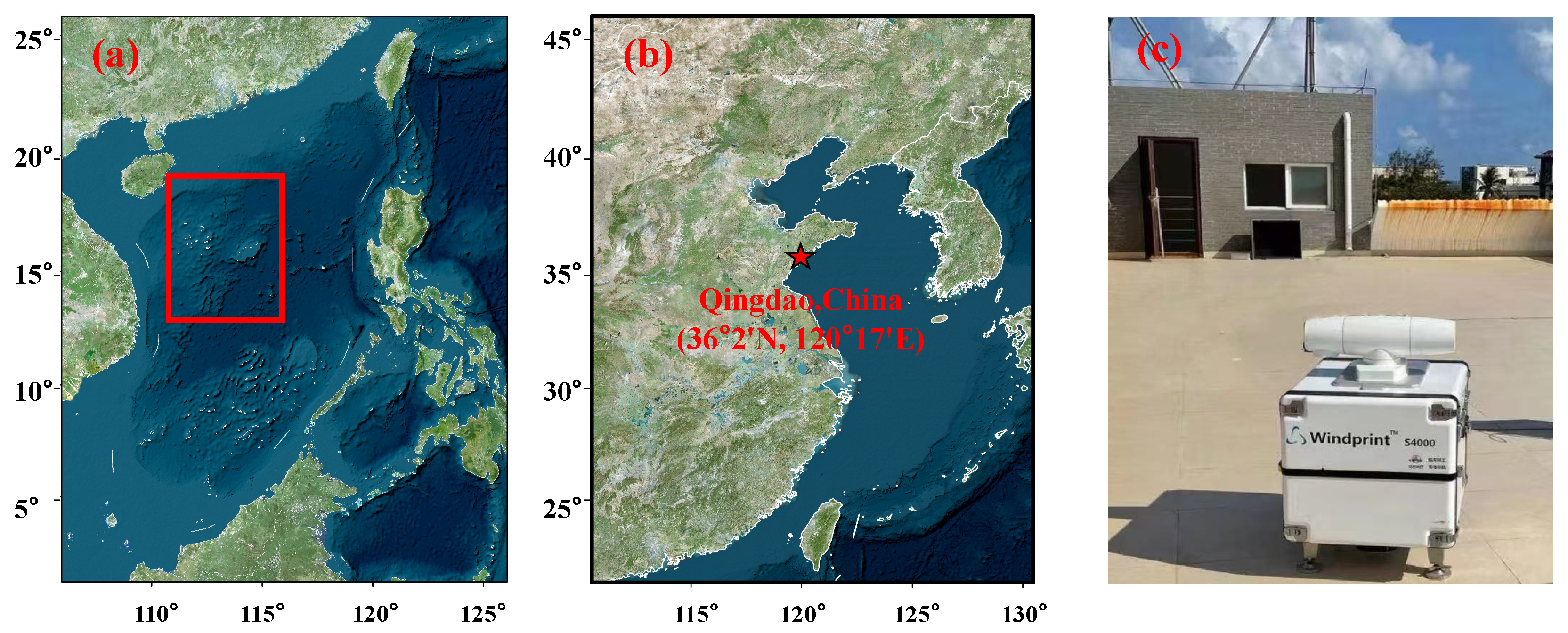
The atmospheric observation experiment site is located in the SCS, as marked by the red rectangle in Figure 1a. The Institute of Optics and Fine Mechanics of the Chinese Academy of Sciences conducted a series of experiments focusing on marine fixed-point wind profiling and shipborne measurements of marine atmospheric turbulence within the SCS from December 2019 to May 2021. To validate the adaptability of the SOEM framework to heterogeneous coastal climates, an atmospheric observation campaign was conducted in Qingdao, Shandong Province, China (36°2′N 120°17′E), from December 2019 to April 2020, as illustrated in Figure 1b.
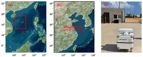
Figure 1.
(a) Study site (red rectangle) in the SCS. (b) Study site in Qingdao. (c) Picture of the Windprint S4000 CDWL during field data collection.
Measurements were carried out using Windprint S4000 CDWL (Qingdao Aerospace Seaglet Environmental Technology Ltd., Qingdao, China), as shown in Figure 1c. CDWL retrieves three-dimensional wind fields through Doppler shift measurements, precisely capturing transient variations in MABLH and providing an independent validation benchmark for the SOEM model. In this setup, the blind size is reduced since the laser beam is coaxial with the telescope axis, and the technical specifications are shown in Table 1. The diameter of the telescope was configured to 40 mm, with a focal length of 1 km. The vertical resolution of this instrument was 30 m, and the temporal resolution, including data sampling and processing, was 4 s. The measurement scheme periodically switched to five directions: north, south, east, west, and vertical. As a result, the data interval for each column was 20 s.

Table 1.
Technical specifications of Windprint S4000 CDWL.
A typical SNR image, which includes 180 successive measurements, is shown in Figure 2a. The SNR of one measurement and the average SNR of the successive 180 measurements are demonstrated in Figure 2b. The MABL is in the range of the red rectangular area, and the aerosol extinction coefficient (AEC) of MABL is homogeneous. This work presents an automated algorithm to extract MABLHs simultaneously. The weather in December was chosen for a typical case to verify the feasibility of the proposed method. The continuous sample data of 24 h obtained by CDWL were used to study the daily evolution of MABLHs and the optical properties of aerosol.
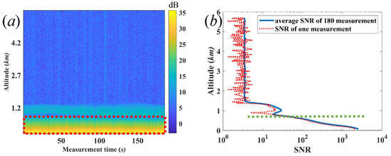
Figure 2.
(a) A typical SNR image of 180 successive measurements; (b) SNR of one measurement, and the average SNR of 180 successive measurements. The MABL is in the red rectangular area. The green dashed line denotes the top of the MABL, which can be considered an MABLH.
2.2. Micro-Pulse Lidar Data
Micro-pulse lidar (MPL), a type of Mie-scattering micro-pulse lidar [41], was utilized for continuous observations of aerosol optical properties during the SCS experiment from June 2019 to December 2020. MPL identifies cloud base heights and the top of the mixed layer through aerosol backscatter coefficient profiles. By synergizing with CDWL observations during comparisons against ERA5 boundary-layer data, this multi-sensor approach addresses the limitations of single-sensor systems in resolving complex atmospheric processes. MPL offered a vertical resolution of 30 m intervals with a temporal resolution of 5 min. The detection range was about 5 km during the day and could reach up to 15 km at night. In this study, the aerosol extinction coefficient was derived from the backscatter signals of the MPL. The planetary BLH (PBLH) was calculated using both the raw signal gradient method and the extinction coefficient gradient method, which supplemented the data obtained from the CDWL.
2.3. ERA5 Data
ERA5 is the European Centre for Medium-Range Weather Forecasts (ECMWF)’s fifth-generation reanalysis dataset for the global climate and weather over the past eight decades [42]. Reanalysis integrates model data with observations from around the world into a globally complete and consistent dataset using the laws of physics. This principle, known as data assimilation, involves optimally combining previous forecasts with newly available observations every 12 h at the ECMWF to generate the best new estimate of the state of the atmosphere. ERA5 provides hourly estimates for a vast number of atmospheric, ocean-wave, and land-surface variables. The data have been regridded to a regular latitude–longitude grid of 0.25° for reanalysis and 0.5° for uncertainty estimation (0.5° and 1° for ocean waves, respectively). The dataset comprises four distinct subsets defined by temporal resolutions (hourly or monthly) and vertical structures: hourly pressure-level products (upper air fields), hourly single-level products (atmospheric, ocean-wave, and land-surface variables), monthly pressure-level products, and monthly single-level products.
The MABL is a critical region for air–sea interactions, with its characteristics influenced by multiple meteorological variables. The selection of these variables for marine atmospheric boundary-layer-height (BLH) quantification is rooted in their capacity to characterize the thermodynamic and dynamic processes governing air mass vertical structure. The impacts of energy–thermodynamic drivers (, , RH, SP, SSH, and STRD) and momentum exchange terms (10U and 10V) on coastal atmospheric BLH estimation exhibit significant variability across distinct meteorological regimes [43]. Sensible heat flux (SHF) is a major factor in the temporal and spatial variations of the BLH [44]. As the concentration of meteorological elements (e.g., cloud cover and aerosols) increases, the sensitivity of the SSR errors of ERA5 to TCC and TP exhibits a significant enhancement [45].
This study focuses on three core processes of MABLH: energy balance, momentum exchange, and vertical structure regulation. A total of 23 variables from ERA5 were selected and categorized into three functional groups: energy and thermodynamic drivers, momentum exchange, and boundary-layer structure and cloud processes. The characteristics of these variables are summarized in Table 2.
Table 2.
The characteristics of 23 variables from ERA5, which were selected and categorized into energy and thermodynamic drivers, momentum exchange, and boundary-layer structure and cloud processes.
3. Materials and Methods
This study focuses on estimating MABLHs in the vicinity of the observation site within the SCS, a region characterized by meteorological sparsity and coupled dynamic–thermodynamic complexity. To address the challenges of data scarcity and intricate physical processes in MABLH prediction, we propose a comprehensive ensemble model framework, termed the stacking optimal ensemble model (SOEM), that integrates multi-source data and artificial intelligence technologies, as shown in Figure 3. The SOEM framework comprises three sequential phases, radar data preprocessing, weather clustering and data assimilation/integration, and SOEM validation and output, each designed to systematically resolve observational limitations and enhance prediction robustness through synergistic data fusion.
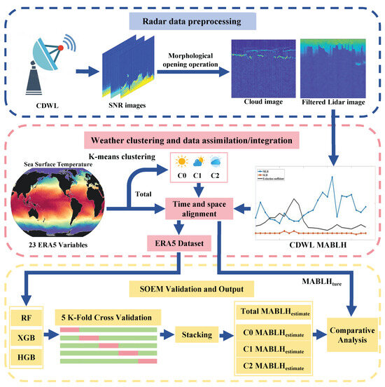
Figure 3.
The framework of the proposed SOEM. C0, clear/slightly cloudy condition; C1, cloudy/transitional condition; C2, overcast/rainy condition.
3.1. Radar Data Preprocessing
CDWL obtains vertical wind speed profiles and aerosol extinction coefficients by emitting laser pulses and receiving backscattered signals. The signal-to-noise ratio (SNR) of CDWL depends mainly on four factors: the average direct detection power, the heterodyne efficiency, the wavelength , and the receiver bandwidth B [1]. Under the conditions of negligible refractive-turbulence effects, the matched filter , where is the pulse duration, and the far-field operation, the peak of the SNR depends on the altitude z and can be expressed as follows [46,47]:
where is the quantum efficiency of the detector, h is the Planck constant, is the transmitting pulse energy, is the backscatter coefficient, and D is the diameter of the laser beam. is the dimensionless one-way irradiance extinction at wavelength , and is the linear AEC along the propagation path.
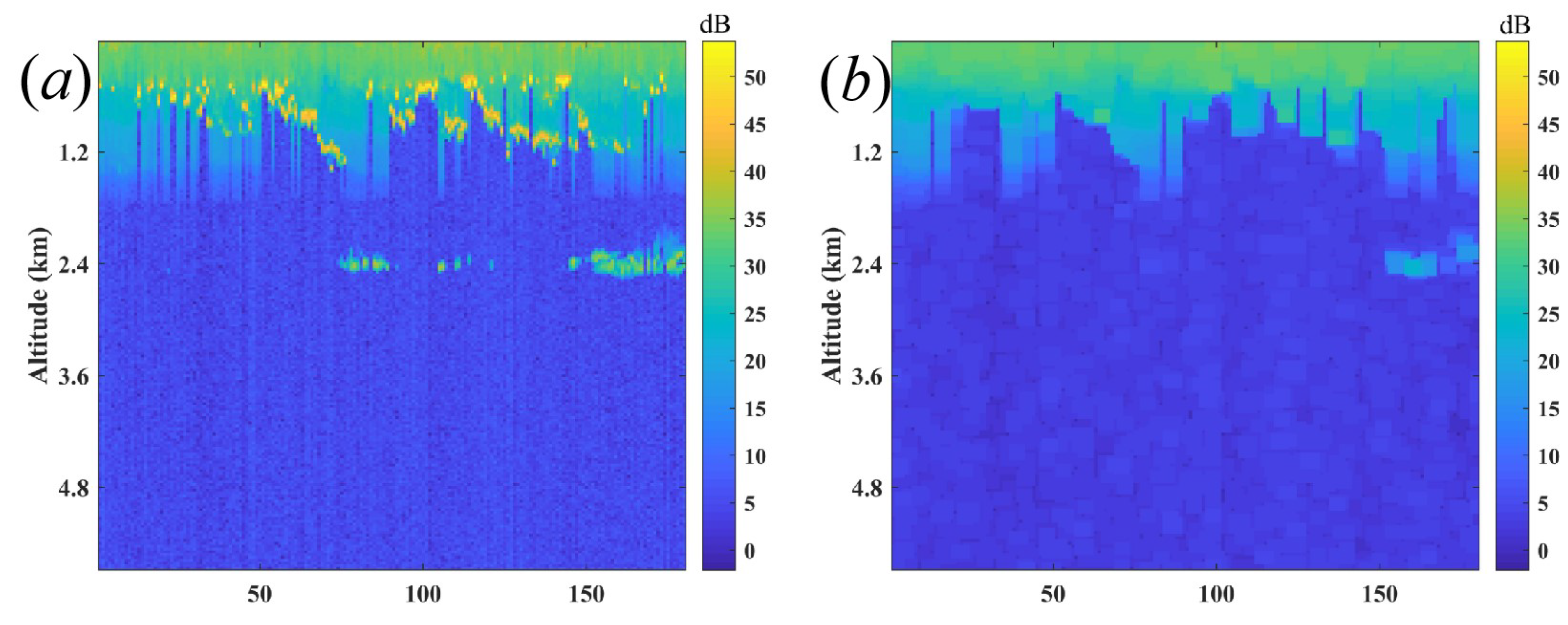
The core methodology for extracting MABLH in this study follows the standardized procedures previously validated by our research team [47,48]. To address the challenge of cloud interference in CDWL SNR images, cloud signals were isolated via a morphological opening operation to generate cloud-removed filtered images. This process effectively eliminates cloud-induced disturbances on signal attenuation patterns while preserving vertical aerosol distribution characteristics within the boundary layer, significantly enhancing data quality, as demonstrated in Figure 4a,b. Subsequently, the Haar wavelet covariance transform combined with an automated dilation algorithm was implemented to precisely identify local extrema in the SNR profiles for determining MLH from the filtered images. The robustness of this methodology has been confirmed through long-term observations at our SCS site and under complex meteorological conditions in Qingdao.

Figure 4.
(a) A lidar image destroyed by clouds; (b) the filtered lidar image with the morphological opening operation.
In marine environments, the presence of a low SNR constitutes a significant challenge. Wavelet threshold denoising can be used to enhance the SNR, separating signals from noise through multi-scale decomposition while preserving turbulent pulsation characteristics. The morphological opening operation is applied to the SNR image to eliminate isolated noise points while preserving the boundaries of the aerosol layers.
3.2. Weather Clustering and Data Assimilation/Integration
The 1 h resolution data from ERA5 are matched to the 10 min resolution of CDWL using bilinear interpolation, effectively addressing the temporal mismatch between ERA5 data and observational data. This spatiotemporal alignment ensures consistency in large-scale meteorological patterns while preserving the unique capability of CDWL to resolve sub-hourly boundary-layer transients.
In the ERA5 dataset, 23 variables were meticulously screened to exclude non-numeric, missing, or outlier data (for example, BLH values of less than 200 m). Subsequently, bivariate linear interpolation was applied, which yielded a refined dataset comprising 47,057 data groups. This preprocessed ERA5 dataset serves as the exclusive input to the SOEM, generating estimated MABLH values (MABLHestimate). The CDWL-derived MABLH (MABLHtrue) acts as an independent benchmark for rigorous validation, leveraging its high-resolution observational fidelity.
To further explore the variations in MABLH in different ABL structures, a K-means clustering algorithm [13] was employed to group the data into homogeneous clusters. This dual-validation framework, combining the broad coverage of ERA5 with the process-scale fidelity of CDWL, ensures the representativeness of the training data across diverse meteorological regimes. Notably, the SOEM excludes CDWL data during training to prevent information leakage, ensuring validation objectivity. The accuracy and robustness of the model were subsequently evaluated by comparing the clustering outcomes with the training results derived from the observed data. The K-means algorithm was strategically applied to the total cloud cover (TCC) of ERA5 to address variable scarcity. This selection emphasizes cloud-driven boundary-layer transitions while maintaining methodological consistency with the aerosol-based retrievals of CDWL [49].
3.3. SOEM Validation and Output
Three base models—RF, XGB, and HGB—were selected and trained on both unclustered and clustered data (cluster 0/1/2). Clustering via K-means enhances computational efficiency by grouping weather regimes with similar thermodynamic profiles. The stacking framework integrates these heterogeneous models to harness their complementary strengths: RF captures nonlinear feature interactions, XGB optimizes gradient pathways, and HGB enables efficient high-dimensional feature processing. This hierarchical design reduces overfitting risks and corrects systematic biases through meta-learning.
The inputs to the SOEM exclusively comprise ERA5 reanalysis variables (e.g., temperature, humidity, wind speed) without incorporating any CDWL-derived MABLH data. The CDWL dataset serves solely as an independent observational benchmark for validating SOEM outputs. ERA5 reanalysis and CDWL observations exhibit complementary roles in validation. ERA5 provides globally consistent estimates of the marine atmospheric boundary-layer height (MABLH) through multi-source data assimilation, acting as a reliable reference for large-scale climate regimes. CDWL captures 10 min interval MABLH transients (e.g., boundary-layer turbulence collapse) with 15 m scale vertical resolution—a capability constrained by the vertical interpolation smoothing effects of ERA5. Cross-validation between model-driven (ERA5) and observation-driven (CDWL) datasets reveals systematic biases while confirming methodological consistency, thereby demonstrating the framework’s robustness.
The dataset was partitioned into training (80%) and testing (20%) sets, with 20% of the training set allocated for hyperparameter validation. We implemented stratified five-fold cross-validation to address class imbalance and high-dimensional feature space challenges, preserving population distributions across folds and ensuring reliable performance estimation and enhanced generalizability.
3.3.1. RF Modeling
The RF Regressor, which is based on the bootstrap aggregating (bagging) algorithm, involves sampling the training set with replacement, thereby dividing different weather types into diverse subsets of samples [50]. During the node-splitting process of each decision tree, the feature dimensions are randomly selected, and the optimal feature is used to split the nodes for estimation. Ultimately, by integrating the predictive results of all subset decision trees and averaging them (denoted as ), the predicted value of the target variable, such as the MABLH, is obtained. This method boasts high robustness, the efficient handling of high-dimensional features, and excellent generalizability. It effectively suppresses noise interference and can directly process the multi-dimensional spatiotemporal data of meteorological elements without feature dimensionality reduction, showing stable performance in predicting extreme weather events and correcting climate models.
3.3.2. XGB Modeling
XGB is a highly efficient ensemble learning algorithm based on the gradient boosting framework [51]. Its core principle lies in iteratively training multiple decision trees, where each tree focuses on correcting the residuals of its predecessor, thereby progressively enhancing the prediction accuracy of target variables (e.g., MABLH). In atmospheric data modeling, XGB demonstrates notable strengths in efficiency, flexibility, and precision. Leveraging parallel computing and sparsity-aware algorithms significantly accelerates the training process on large-scale meteorological datasets. Additionally, its support for customizable loss functions and regularization terms enables effective adaptation to nonlinear relationships and complex physical mechanisms inherent in atmospheric data. XGB has shown exceptional performance in extreme weather event prediction and climate model correction, particularly excelling in handling high-dimensional features.
3.3.3. HGB Modeling
HGB is a gradient boosting algorithm that utilizes histogram binning to discretize continuous features, thereby reducing computational complexity and accelerating model training [52]. In atmospheric data modeling, Hist offers several advantages, including high computational efficiency, low memory consumption, and strong robustness. These characteristics make it particularly suitable for processing high-resolution meteorological data, while its insensitivity to noise and outliers ensures the stable handling of uncertainties in atmospheric datasets.
3.3.4. Stacking Modeling
The stacking modeling framework enhances atmospheric data modeling performance through the hierarchical integration of complementary heterogeneous base models [53]. Our implementation includes three base learners: Random forest (RF) captures nonlinear interactions, XGBoost (XGB) optimizes gradient paths, and histogram-based gradient boosting (HGB) accelerates feature binning. The five-fold cross-validation generates meta-features, ensuring that base model predictions remain independent of the training data to prevent information leakage.
A modified histogram-based gradient boosting model serves as the meta-learner. Its nonlinear splitting mechanism dynamically reweights base models and compensates for systematic biases. Hierarchical hyperparameter optimization isolates base model tuning from meta-model configurations to avoid objective conflicts.
Finally, the performance of the stacked model was rigorously evaluated on the testing set, demonstrating its ability to enhance prediction accuracy and robustness compared to individual models, particularly in capturing complex atmospheric phenomena such as MABLH variations and extreme weather events.
3.4. Evaluation Indicators
To comprehensively evaluate the performance of SOEM in the estimation of MABLH, we performed a tripartite comparison between lidar-derived MABLHs() and SOEM-generated estimates (). The evaluation framework incorporates multiple statistical metrics to address different aspects of model performance. The root mean square error (RMSE) quantifies the overall magnitude of the deviation while emphasizing larger errors. The mean absolute error (MAE) provides robust dispersion measurement. The mean absolute percentage error (MAPE) evaluates the relative error distribution. The coefficient of determination () assesses the explained variance:
where N denotes the sample size, superscript i indicates the ith measurement, and represents the observational mean. This multi-metric approach combines error magnitude analysis (RMSE/MAE), relative error assessment (MAPE), and variance explanations () to rigorously evaluate model performance. Five-fold stratified cross-validation and bilinear spatiotemporal interpolation guarantee statistical robustness, the RMSE/MAE ratio quantifies the outlier impacts and -MAPE, and anticorrelation reveals scale-dependent performance degradation. This integrated methodology overcomes individual metric limitations by synergistically resolving absolute errors, relative deviations, variance attribution, and regime-specific biases.
4. Results
4.1. Model Evaluation
This study employs a K-means clustering algorithm to decouple complex meteorological conditions into subclasses with distinct physical characteristics, revealing the dynamic–thermal coupling mechanisms in boundary-layer structures under varying cloud coverage conditions. As shown in Table 3, the total sample size of 43,037, which was not subjected to TCC-based clustering, is denoted as “Total”. When K = 3, the Silhouette score was 0.65, and the Calinski–Harabasz score was 25,6750.46, effectively distinguishing meteorological states under different cloud conditions. Specifically, Cluster 0 (TCC < 0.336) represents the clear/slightly cloudy condition, corresponding to a stable boundary layer dominated by radiative cooling (such as at night or under anticyclonic control), and it is denoted as “C0”. Cluster 1 (0.336 ≤ TCC < 0.729) represents the partially cloudy/transitional condition, potentially accompanied by stratocumulus clouds or frontal passages, with the boundary layer influenced by dynamic (wind shear) and thermal (entrainment) processes; it is denoted as “C1”. Cluster 2 (TCC ≥ 0.729) represents overcast/rainy, potentially corresponding to strong convection or persistent stratiform clouds, where the PBLH is suppressed or lifted by the radiative cooling of the top of the cloud; it is denoted as “C2”. The number of filtered samples for each cluster was 14,738, 17,227, and 11,072, respectively.
Table 3.
Results of four machine learning models.
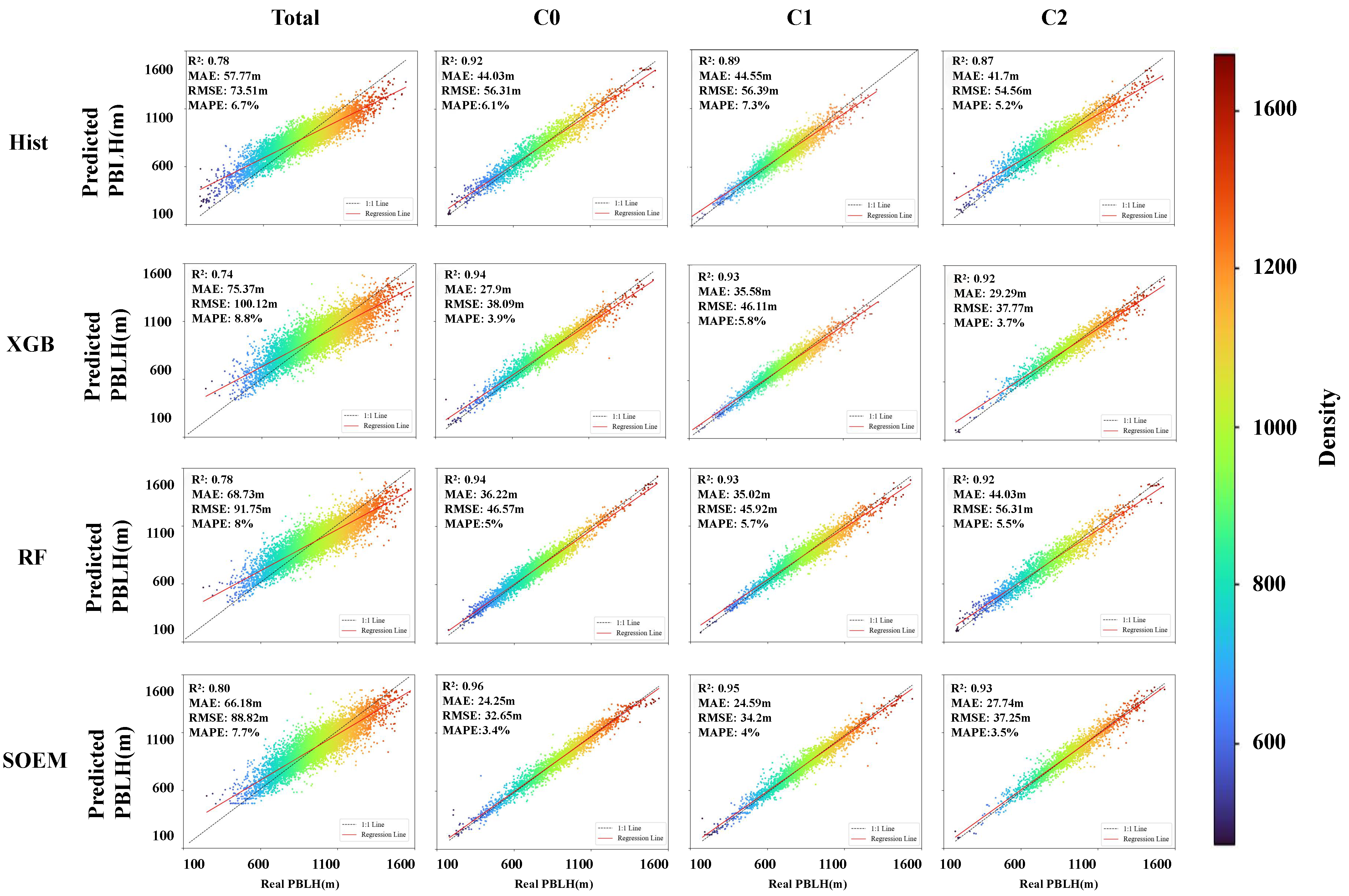
To evaluate whether the introduction of clustering technology enhances the predictive performance of the model and the performance of the integrated SOEM, we first compared it with baseline models such as HGB, XGB, RF, and SOEM. Table 3 presents the evaluation results of these four models for estimating MABLH. The results indicate that introducing clustering technology significantly improves the model’s predictive performance. By dividing the data into subsets corresponding to different meteorological conditions, the model can better adapt to specific conditions, thereby enhancing the accuracy and robustness of the predictions.
Figure 5 presents the results of the MABLH predictions of the HGB, XGB, RF, and SOEM models against the observations measured by CDWL. After clustering, the MAE fluctuation range is significantly reduced for all models. It is worth noting that the MAE is reduced from 66.18 m (Total) to 24.25 m (C0), 24.59 m (C1), and 27.75 m (C2) for the SOEM model. This indicates that the predictive performance of the model is more stable under different meteorological conditions. The SOEM shows an average improvement of 12% in and 22% in the MAE over other models in complex meteorological environments. The SOEM achieves an average MAPE of 3.7% for the MABLH estimation, reducing the error by 37.7% compared to ERA5 products. Under conditions C0, C1, and C2, SOEM demonstrates an average RMSE of 34.45 m (42.9% reduction) and MAPE values of 6.18%, 6.3%, and 7%, whereas ERA5 has higher errors of 10.2%, 10.3%, and 10.4%, highlighting the critical role of clustering technology for model stability under different meteorological conditions.
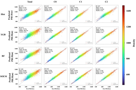
Figure 5.
Results of MABLH predictions from HGB, XGB, RF, and SOEM models against the observations measured by CDWL.
The RF model demonstrates robust predictive performance in all cluster scenarios, characterized by high values and low MAE values. This indicates the effectiveness of the model in capturing the underlying patterns and mixed meteorological conditions. The model achieves its lowest MAE in C1 (35.02 m), benefiting from the bagging strategy that reduces variance and adapts to the stochastic nature of parameter fluctuations under transitional conditions. However, its MAE in C2 increases sharply to 44.03 m, potentially due to the failure of individual tree-splitting rules under multimodal input parameter distributions (such as vertical wind speed and cloud water content) under cloudy conditions.
XGB exhibits a polarization phenomenon, performing best in C0 (MAE = 27.9 m) and C2 (MAE = 29.29 m), as its boosting mechanism is more sensitive to the ranking of feature importance under stable conditions (clear sky) and strong constraint conditions (cloud-top inhibition). However, it has the lowest in the overall (Total) scenario, reflecting the model’s difficulty in balancing conflicting patterns under unclustered meteorological conditions.
The HGB model maintains relatively high performance in the overall (Total) scenario due to its computational efficiency and ability to prevent overfitting. However, when faced with complex and heterogeneous data patterns in this study, the HGB model is less flexible than the RF and XGB models, with the highest reaching 0.92.
In contrast, the SOEM dynamically assigns weights to base models through a meta-learner (such as linear regression), achieving an of 0.96 in the C0 scenario, which is a 2% improvement compared to the best single model ( of the RF model). Switching dominant physical processes under different meteorological conditions requires the predictive model to possess “dynamic expert” characteristics. The SOEM constructs a “conditional ensemble” framework by training sub-models after clustering, demonstrating its superior predictive performance.
4.2. Temporal Characteristics of Prediction Errors in the SOEM and ERA5
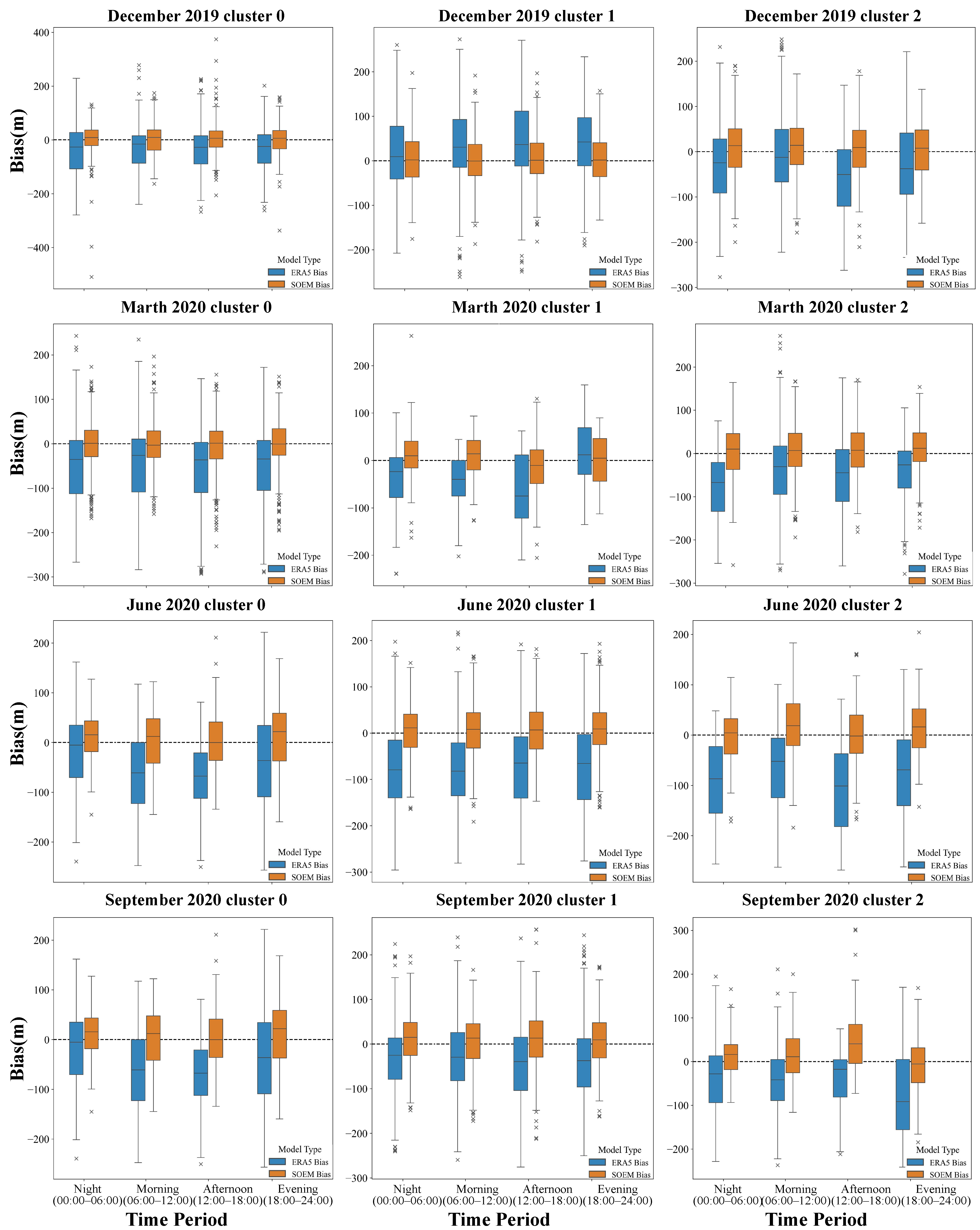
To elucidate seasonal variations in temporal error characteristics between BLH, , and , this study analyzed observational data under different synoptic conditions (C0, C1, and C2) at representative stations during four crucial climatic months: December 2019 (winter), March 2020 (spring), June 2020 (summer), and September 2020 (autumn).
As shown in Figure 6, statistical validation demonstrates that the SOEM, which integrates physics-constrained machine learning, achieves significantly higher accuracy than the traditional reanalysis dataset ERA5 in retrieving MABLH over the SCS under all weather conditions. Bias distributions across synoptic regimes (C0/C1/C2) reveal critical error mechanisms; under the C0 condition, SOEM exhibits a higher median bias (MED) and higher interquartile range (IQR) compared to the C1 and C2 conditions. The minimum IQR of 21.2 m observed in March 2020 confirmed the stability of the model during the transitional seasons. ERA5_bias shows a negative skewness in 93% of the cases (MED = −101.1 m in summer C2), with an elevated IQR (mean = 62.3 m), reflecting the decoupling effects of parameterization schemes from multi-scale air–sea interactions. The static Charnock coefficient in ERA5 fails to capture tidal-modulated momentum flux transients, leading to underestimated afternoon sensible heat fluxes and the delayed simulation of boundary-layer collapse.
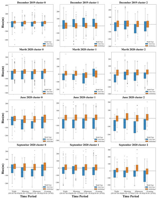
Figure 6.
Temporal characteristics of prediction errors in SOEM and ERA5.
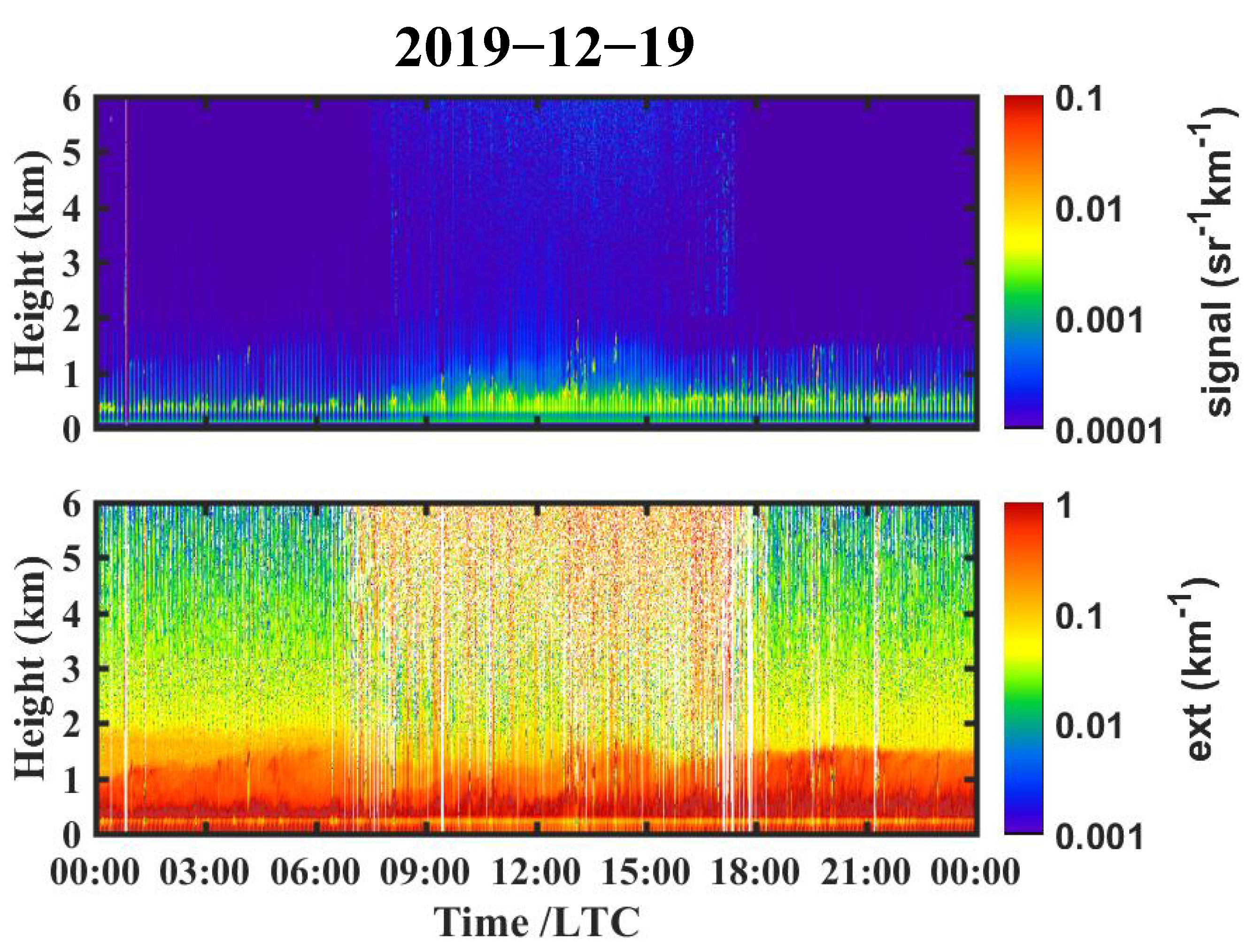
The seasonal bias characteristics at the monitoring site are governed by monsoon–sea surface temperature configurations, with pronounced negative biases during summer and autumn nights, contrasting with smaller biases in spring and winter. This pattern correlates directly with phase lags in latent heat flux during monsoon transitions. MPL lidar observations confirm that MABLH diurnal variability is generally subdued compared to terrestrial sites (except under C2 conditions), which is attributed to oceanic thermal inertia. The weak disequilibrium in turbulent kinetic energy budgets between day and night results in flattened diurnal cycles, as shown in Figure 7.
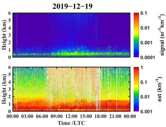
Figure 7.
Spatiotemporal distribution of echo signals (Top) and BLH (Bottom) observed by MPL on 19 December 2019.
This study demonstrates that in dynamically complex regions such as the SCS, where multi-scale processes interplay, traditional global models (e.g., ERA5) fail to predict boundary-layer dynamics due to the inadequate parameterization of oceanic subgrid processes and decoupled regional thermal forcing. In contrast, the novel SOEM employs a fully coupled cloud–boundary-layer architecture, translating intricate environmental factors into physics-informed constraints, thereby substantially enhancing predictive reliability.
4.3. Capability of Detecting Anomalous Weather
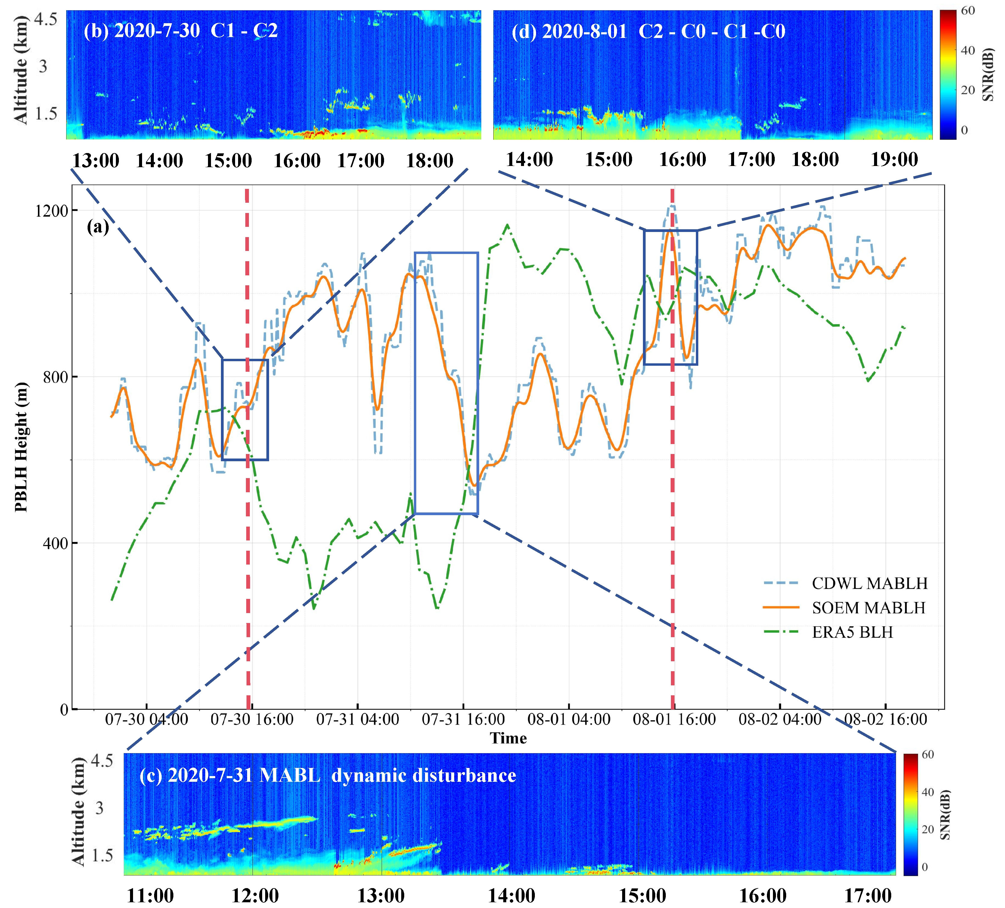
Figure 8 systematically demonstrates the co-evolution of MABLH and SNR during Typhoon Sinlaku’s passage over the SCS in 2020. Benefiting from its high vertical resolution (30 m), CDWL precisely resolved aerosol-layer discontinuities characterized by steep SNR gradients.

Figure 8.
Co-evolution of MABLH and SNR during Typhoon Sinlaku’s passage over the Study Site in 2020. (a) Intercomparison of MABLH time series derived from CDWL, ERA5 reanalysis, and SOEM. (b) Approaching Phase: SNR evolution and synoptic pattern transition (C1–C2). (c) Passing Phase: MABL dynamic disturbance. (d) Departing Phase: SNR evolution and synoptic pattern transition (C2–C0–C1). Two red vertical dashed lines demarcate typhoon transit phases: Approaching Phase–Passing Phase–Departing Phase.
Figure 8a compares the MABLH time series derived from CDWL, ERA5 reanalysis, and SOEM from 30 July to 2 August 2020. The SOEM MABLH exhibited a strong correlation with CDWL observations in capturing the three-stage evolution (Approaching Phase, Passing Phase, and Departing Phase) of the typhoon-induced boundary-layer dynamics, particularly revealing a distinct bimodal structure in MABLH during this event. In contrast, ERA5 BLH demonstrated significant phase lag (6~7 h) and systematic underestimation.
Figure 8b corresponds to the pre-approval phase transition (13:00–18:00 LT, 30 July), depicting SNR evolution and synoptic pattern shifts (C1–C2). As the typhoon’s outer rainbands progressively enveloped the region, the cloud systems evolved from cirrus to cumulonimbus with thickening cloud layers and intermittent heavy precipitation, causing the elevation in MABLH from 600 m to 850 m.
Figure 8c captures MABL dynamic disturbance during the Passing Phase (11:00–17:00 LT, 31 July), triggered by extreme synoptic variability. Through temporal correlation clustering (TCC) and physics-constrained loss functions, the SOEM accurately resolved the abrupt MABLH collapse from 1087 m to 476 m.
Figure 8d illustrates the post-Departing Phase transition (14:00–19:00 LT, 1 August), characterized by decaying trailing rainbands, subsidence-dominated regimes, and cloud dissipation. As precipitation gradually stopped, the synoptic pattern reverted from C2 to the C0/C1 states.
This study establishes an observation–model-coupled framework to quantify typhoon–boundary-layer interactions, offering a novel paradigm for optimizing marine boundary-layer parameterization under extreme weather.
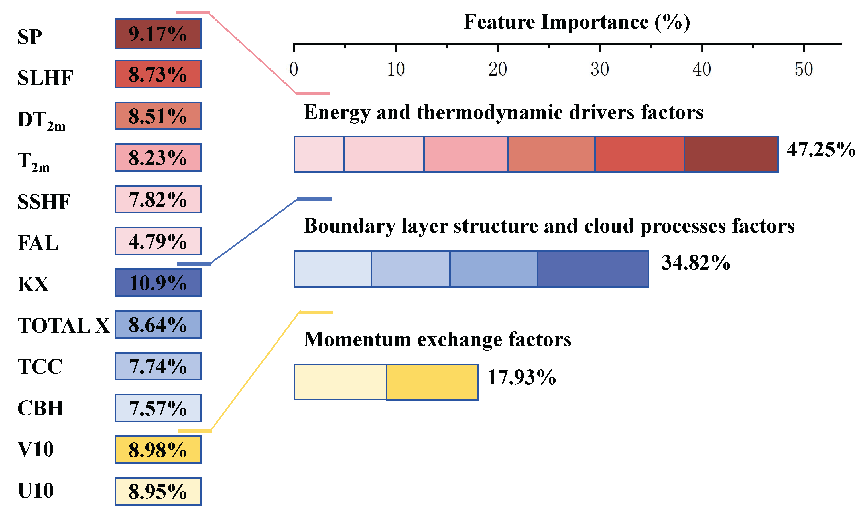
4.4. Feature Importance Analysis
To identify the key drivers of MABLH variability, Shapley Additive exPlanations (SHAP) analysis was applied to 23 ERA5 parameters (excluding BLH), and 12 dominant drivers were selected. Figure 9 demonstrates that the thermodynamic parameters (, , SLHF, and SSHF) dominate feature importance, accounting for 47.25% of the total contribution. MABLH is primarily driven by latent heat flux (SLHF), with a correlation coefficient as high as 0.8, validating the “latent-heat-dominant” thermal characteristic of the oceanic boundary layer. The dynamic parameters (U10 and V10) collectively contribute 34.82% to the importance and exhibit threshold responses, with correlations that decay significantly when wind speeds exceed −10 m/s. Cloud- and boundary-layer structural parameters (CBH, TCC, TOTAL X, SP, FAL, and KX) account for 17.93% of the total importance. Notably, the negative correlations () between the cloud/precipitation parameters (TCC and TOTAL X) highlight the triadic interactions among radiation, turbulence, and phase transitions.
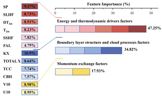
Figure 9.
Drivers of MABLH variability.
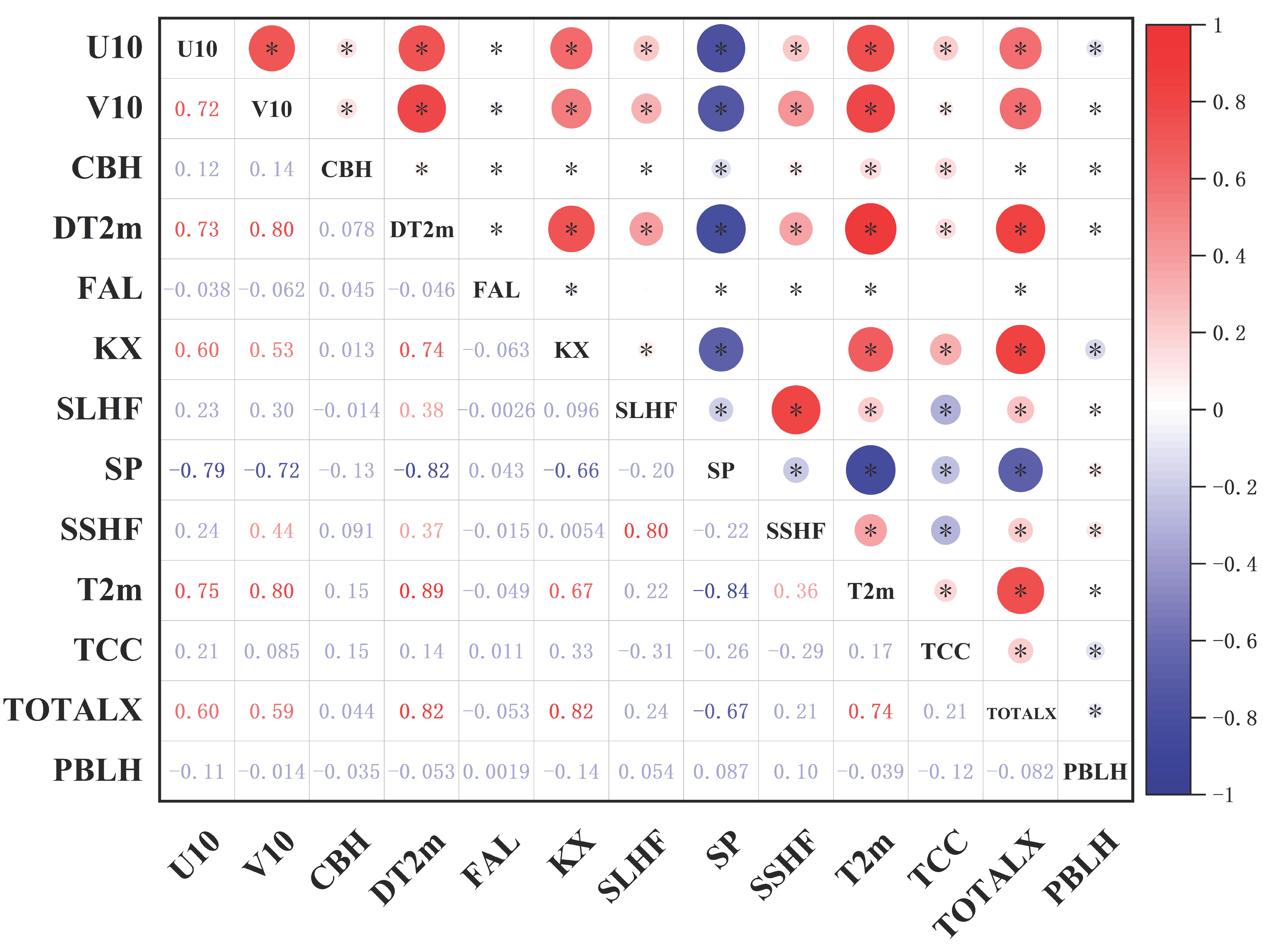
Figure 10 shows the thermodynamic matrix of parameter–PBLH interactions with statistical significance tests. Strong positive correlations between PBLH and KX (), TCC (), and U10 () highlight the dominance of thermal and mechanical turbulence in the development of the boundary layer. enhances near-surface instability, driving convective updrafts that expand the PBLH. Similarly, high wind speeds (U10/V10) generate mechanical turbulence, increasing vertical mixing. In contrast, the strong negative correlation with SP () reflects the suppression of PBLH in high-pressure systems, where subsidence and stable stratification inhibit turbulent energy. These relationships align with the classical boundary-layer theory, where thermal forcing and wind shear jointly regulate PBL growth, revealing two distinct regimes that govern MABLH.
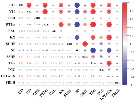
Figure 10.
Correlation matrix of MBL parameters. ∗ denotes statistical significance (p < 0.01). The heatmap color gradient represents Pearson correlation coefficients, with red/blue indicating positive/negative correlations.
Weak statistically significant correlations (for example, FAL-PBLH: ; and TOTAL X-PBLH: ) may arise from indirect mechanisms or dataset properties. For aerosols (FAL/TOTAL X), slight negative links could stem from radiative effects: elevated aerosol layers may reduce surface heating by scattering solar radiation, subtly dampening convective energy. Although these correlations are statistically significant () due to large sample sizes, their minimal magnitude suggests limited physical influence compared to dominant drivers such as . This underscores the need to distinguish statistical significance from practical relevance in interpreting atmospheric correlations.
5. Discussion
5.1. Generalization of Weather Regime Clustering
The SOEM framework, though optimized for MABLH retrieval in the SCS, demonstrates promising but constrained generalizability across diverse climatic regimes. Notably, the CDWL-derived MABLH serves as the ground truth of the comparative analysis of the SOEM, with the model’s accuracy fundamentally rooted in active remote sensing measurements from the SCS.
Through systematic validation conducted during the fourth quarter of 2024 in three representative marine regions—the tropical monsoon-dominated western Pacific (Naha, Okinawa), the California current-influenced eastern Pacific (San Diego), and the Mediterranean climate zone (Athens)—classification accuracies of 70.2%, 68%, and 63% were achieved, respectively.
However, the absence of CDWL observations in these regions necessitated reliance on ERA5 reanalysis TCC parameters for weather regime clustering, which is a methodological adaptation that evaluates synoptic pattern adaptability rather than strict geographic–climatic validation.
These results align with previous studies on unsupervised learning in weather pattern recognition while also revealing region-specific limitations. In an investigation of tropical convective clouds, Kim et al. (2023) implemented a computer vision-based segmentation framework to isolate meteorological entities exhibiting divergent cloud characteristics [44]. Their self-organizing map-clustering method achieved a regional consistency rate of 70% in diverse periods. However, this performs poorly compared to the 81.7% consistency reported in Qingdao tests, likely due to the univariate TCC clustering’s failure to account for significant thermodynamic divergence between marine climate subtypes. The discrepancies are mainly due to transitional weather processes (e.g., discontinuities in typhoon rainbands), contributing to 30% of misclassifications in tropical margins and underscoring the necessity for adaptive feature engineering.
5.2. Validation Conducted in Qingdao, China
Situated within the Bohai Sea temperate monsoon zone, Qingdao exhibits distinctive land–sea interactions: Winter temperatures (−16 °C to 5 °C) are modulated by the northerly transport of industrial pollutants, and summer convective systems are driven by Yellow Sea cyclonic activity under high-humidity conditions. The winter aerosol regime is dominated by hybrid particles from Bohai marine salts and anthropogenic emissions from coal-fired heating systems, generating complex boundary-layer stratification.
As summarized in Table 4, the unclustered dataset (“Total”) comprises 16,419 samples. K-means clustering (K = 3) achieved optimal class separation with a Silhouette score of 0.61 and a Calinski–Harabasz score of 129,478.23, successfully categorizing meteorological states under distinct cloud regimes. The resulting clusters (C0, C1, and C2) contained 5469, 7618, and 3332 filtered samples, respectively.
Table 4.
Performance comparison of four machine learning models for estimating MABLH in the Qingdao coastal region.
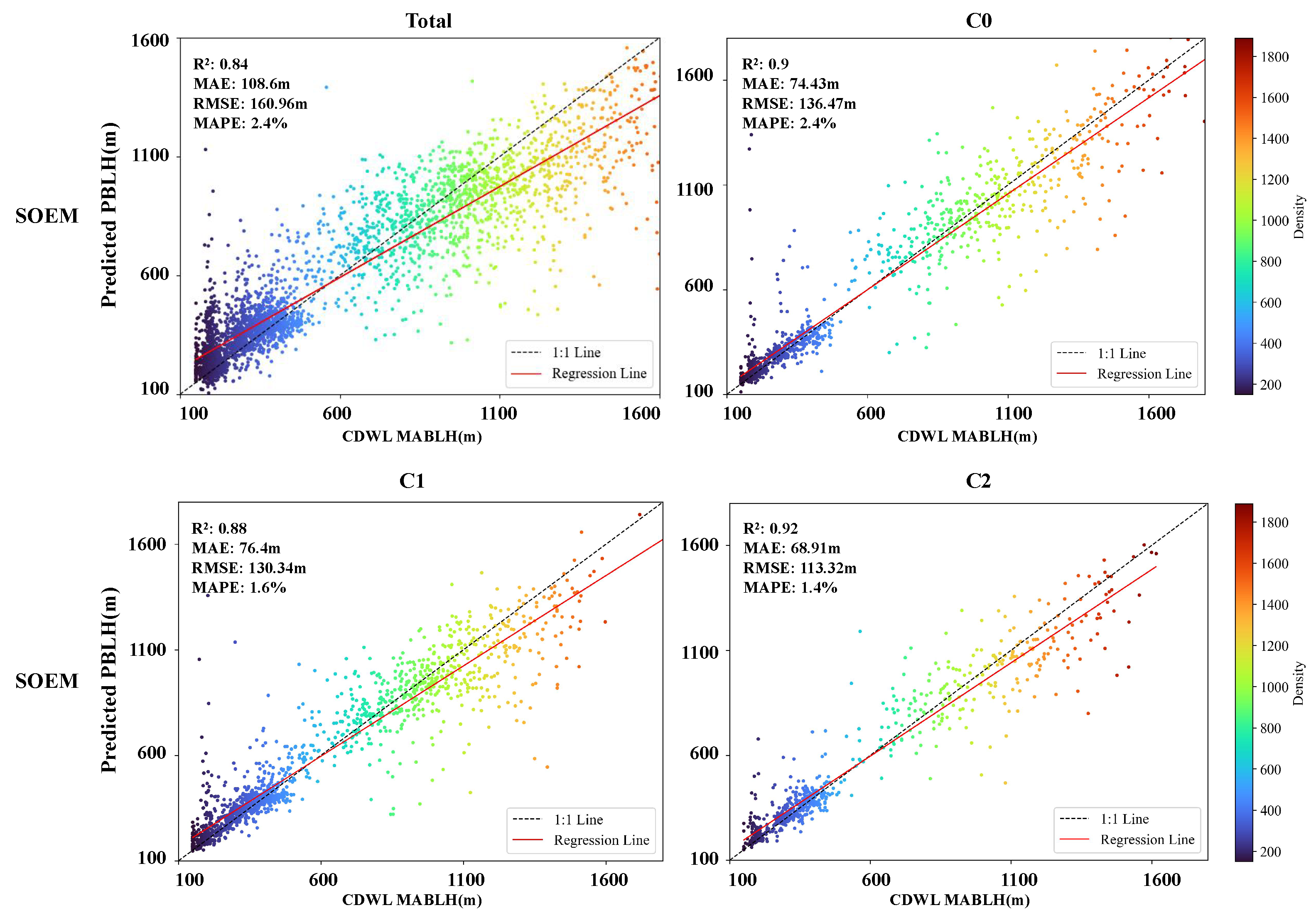
As shown in Table 4, the SOEM framework demonstrates robust performance in Qingdao’s dynamically complex boundary-layer environment. Primarily, SOEM outperforms other baseline models under both clustered and non-clustered scenarios, validating its ensemble optimization efficacy through multi-learner synergy. Notably, the non-clustered configuration (“Total”) achieves with MAE = 108.6 m, while weather-regime-specific clustering further enhances precision across all subcategories. This performance hierarchy conclusively demonstrates the necessity of meteorological regime-aware modeling, particularly in coastal zones where aerosol–cloud interactions dominate boundary-layer evolution.
Figure 11 shows the MABLH predictions from the HGB, XGB, RF, and SOEM models against the observations measured in Qingdao, China. The clustered validation reveals optimal performance for regime C2 (3332 samples), with = 0.92 (MAE 68.91 m), while regime C0 in the SCS achieves = 0.96, with 14,738 samples. The result highlights the framework’s capacity to resolve multi-scale meteorological processes, particularly in data-sparse coastal environments where aerosol–cloud interactions amplify boundary-layer variability. The adaptability of SOEM to limited training samples through adaptive feature reweighting and regime-specific physical parameterization underscores its operational viability in observation-constrained marine zones.
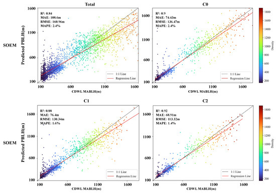
Figure 11.
Results of MABLH predictions from the HGB, XGB, RF, and SOEM models against the observations measured by CDWL in Qingdao, China.
Although current validation is limited to station-adjacent waters, the established framework enables future scalability. Planned expansions incorporate multi-station CDWL and CALIPSO satellite lidar to assess monsoon-driven spatial heterogeneity. These findings underscore the need to develop regionally adaptive MABLH retrieval frameworks. Future research directions should focus on three key improvements: (1) The integration of multi-source heterogeneous data, including coherent CDWL and microwave radiometer observations, to enhance spatialtemporal resolution; (2) the development of graph neural network (GNN)-based spatiotemporal correlation models to address characterization challenges in transitional weather processes; (3) the implementation of transfer learning frameworks to mitigate domain shifts caused by climatic regime disparities, coupled with embedding multi-condition adaptive parameters (e.g., turbulent kinetic energy dissipation rate and gradient Richardson number Ri) as physical constraints into loss functions for improved dynamical consistency in cross-scale interactions.
6. Conclusions
This study proposes a novel SOEM to address the challenge of real-time MABLH retrieval in the data-sparse regions of the SCS. By integrating ERA5 reanalysis data with high-resolution CDWL observations, the SOEM framework incorporates dynamic K-means clustering based on TCC to classify weather conditions into three distinct regimes: clear/slightly cloudy condition (C0), cloudy/transitional condition (C1), and overcast/rainy condition (C2). The model synergizes machine learning techniques, including RF, XGB, HGB, and stacking, to adaptively optimize the feature weights in weather scenarios. The validation results demonstrate that the SOEM achieves an average MAPE of 3.7%, which is significantly lower than conventional ERA5 planetary boundary-layer height products across diverse meteorological conditions. Physical constraints derived from SHAP analysis reveal that energy–thermodynamic drivers, momentum–boundary-layer interactions, and cloud processes collectively govern model performance.
The SOEM outperformed RF, XGB, and HGB models under clear/slightly cloudy conditions, achieving an of 0.95 and an MAE of 32 m. During Typhoon Sinlaku (2020), the predictions of SOEM aligned well with CDWL observations, capturing dynamic disturbances in MABLH. Validation in the coastal city of Qingdao further confirmed the superiority of the SOEM in resolving meteorological heterogeneity.
The validations in the weather clustering algorithm across four regions (Qingdao, Naha, San Diego, and Greece) demonstrated that single-variable clustering based on ERA5 TCC reduced regional consistency from 81.7% to 63%, necessitating multi-physical-variable collaborative clustering. The SOEM framework validated in Qingdao achieved an MABLH inversion accuracy of = 0.92 through K-means regime classification optimization, representing a 9.52% improvement over non-clustered scenarios, thereby confirming its effectiveness in coastal data-sparse regions.
The proposed SOEM framework provides a feasible technical solution for estimating MABLH in data-sparse maritime regions. Its core innovation introduces regime-adaptive optimization via TCC-based weather clustering to resolve coastal meteorological heterogeneity; furthermore, it develops a CDWL-ERA5 synergistic paradigm that compensates observational sparsity through multi-source data fusion. This advancement advances marine weather forecasting accuracy, strengthens early warning capabilities for ocean disasters, and delivers boundary-layer data for air–sea interaction studies in coastal protection engineering.
Author Contributions
Conceptualization, T.L., W.Z. and N.W.; data curation, T.L., G.S. and Q.L.; formal analysis, Y.C., W.Z. and Y.L.; funding acquisition, Y.C., X.J. and N.W.; investigation, Y.C. and Y.L.; methodology, Y.C., T.L., W.Z., X.J. and N.W.; resources, T.L., G.S., W.Z. and Q.L.; software, Y.C.; supervision, G.S.; validation, Y.C.; visualization, Y.C., Q.L., Y.L. and X.J.; writing—original draft, Y.C.; writing—review and editing, T.L., W.Z., X.J. and N.W. All authors have read and agreed to the published version of the manuscript.
Funding
This research was funded by the Anhui Provincial Science and Technology Program (Grant No. O53AG11601), the Research Fund of the State Key Laboratory of Pulsed Power Laser Technology (Grant No. SKL2023ZZ03), and the Natural Science Foundation of Anhui Higher Education Institutions of China (Grant No. KJ2021A1161).
Data Availability Statement
The data are not publicly available due to the requirement that the underlying data of the results presented in this study may only be obtained from the authors upon reasonable request.
Conflicts of Interest
The authors declare no conflicts of interest.
References
- Stull, R.B. (Ed.) An Introduction to Boundary Layer Meteorology; Springer: Dordrecht, The Netherlands, 1988. [Google Scholar] [CrossRef]
- Edwards, J.M.; Beljaars, A.C.; Holtslag, A.A.; Lock, A.P. Representation of Boundary-Layer Processes in Numerical Weather Prediction and Climate Models. Bound. Layer Meteorol. 2020, 177, 511–539. [Google Scholar] [CrossRef]
- Davy, R. The climatology of the atmospheric boundary layer in contemporary global climate models. J. Clim. 2018, 31, 9151–9173. [Google Scholar] [CrossRef]
- Eastman, R.; Mccoy, I.L.; Wood, R. Environmental and internal controls on lagrangian transitions from closed cell mesoscale cellular convection over subtropical oceans. J. Atmos. Sci. 2021, 78, 2367–2383. [Google Scholar] [CrossRef]
- Yang, H.; Chen, Z.; Sun, S.; Li, M.; Cai, W.; Wu, L.; Cai, J.; Sun, B.; Ma, K.; Ma, X.; et al. Observations Reveal Intense Air-Sea Exchanges Over Submesoscale Ocean Front. Geophys. Res. Lett. 2024, 51, e2023GL106840. [Google Scholar] [CrossRef]
- Von Engeln, A.; Teixeira, J. A planetary boundary layer height climatology derived from ECMWF reanalysis data. J. Clim. 2013, 26, 6575–6590. [Google Scholar] [CrossRef]
- Jin, W.; Liang, C.; Hu, J.; Meng, Q.; Lü, H.; Wang, Y.; Lin, F.; Chen, X.; Liu, X. Modulation effect of mesoscale eddies on sequential typhoon-induced oceanic responses in the South China sea. Remote Sens. 2020, 12, 3059. [Google Scholar] [CrossRef]
- Krishnamurthy, R.; Newsom, R.K.; Berg, L.K.; Xiao, H.; Ma, P.L.; Turner, D.D. On the estimation of boundary layer heights: A machine learning approach. Atmos. Meas. Tech. 2021, 14, 4403–4424. [Google Scholar] [CrossRef]
- Dang, J.; Xie, X.; Wen, X. Evaluation of Boundary Layer Characteristics at Mount Siâ˘AZ´ e Based on UAV and Lidar Data. Remote Sens. 2024, 16, 3816. [Google Scholar] [CrossRef]
- Wang, G.; Chen, J.; Xu, J.; Yun, L.; Zhang, M.; Li, H.; Qin, X.; Deng, C.; Zheng, H.; Gui, H.; et al. Atmospheric Processing at the Sea-Land Interface Over the South China Sea: Secondary Aerosol Formation, Aerosol Acidity, and Role of Sea Salts. J. Geophys. Res. Atmos. 2022, 127, e2021JD036255. [Google Scholar] [CrossRef]
- Jin, X.; Song, X.; Yang, Y.; Wang, M.; Shao, S.; Zheng, H. Estimation of turbulence parameters in the atmospheric boundary layer of the Bohai Sea, China, by coherent Doppler lidar and mesoscale model. Opt. Express 2022, 30, 13263. [Google Scholar] [CrossRef]
- Wang, L.; Yuan, J.; Xia, H.; Zhao, L.; Wu, Y. Marine Mixed Layer Height Detection Using Ship-Borne Coherent Doppler Wind Lidar Based on Constant Turbulence Threshold. Remote Sens. 2022, 14, 745. [Google Scholar] [CrossRef]
- Rieutord, T.; Aubert, S.; MacHado, T. Deriving boundary layer height from aerosol lidar using machine learning: KABL and ADABL algorithms. Atmos. Meas. Tech. 2021, 14, 4335–4353. [Google Scholar] [CrossRef]
- de Arruda Moreira, G.; Sánchez-Hernández, G.; Guerrero-Rascado, J.L.; Cazorla, A.; Alados-Arboledas, L. Estimating the urban atmospheric boundary layer height from remote sensing applying machine learning techniques. Atmos. Res. 2022, 266, 105962. [Google Scholar] [CrossRef]
- Rey-Sanchez, C.; Wharton, S.; Vilà-Guerau de Arellano, J.; Paw U, K.T.; Hemes, K.S.; Fuentes, J.D.; Osuna, J.; Szutu, D.; Ribeiro, J.V.; Verfaillie, J.; et al. Evaluation of Atmospheric Boundary Layer Height From Wind Profiling Radar and Slab Models and Its Responses to Seasonality of Land Cover, Subsidence, and Advection. J. Geophys. Res. Atmos. 2021, 126, e2020JD033775. [Google Scholar] [CrossRef]
- Millard, K.; Richardson, M. Quantifying the relative contributions of vegetation and soil moisture conditions to polarimetric C-Band SAR response in a temperate peatland. Remote Sens. Environ. 2018, 206, 123–138. [Google Scholar] [CrossRef]
- Wu, N.; Ding, X.; Wen, Z.; Chen, G.; Meng, Z.; Lin, L.; Min, J. Contrasting frontal and warm-sector heavy rainfalls over South China during the early-summer rainy season. Atmos. Res. 2020, 235, 104693. [Google Scholar] [CrossRef]
- Chen, F.; Kusaka, H.; Bornstein, R.; Ching, J.; Grimmond, C.S.; Grossman-Clarke, S.; Loridan, T.; Manning, K.W.; Martilli, A.; Miao, S.; et al. The integrated WRF/urban modelling system: Development, evaluation, and applications to urban environmental problems. Int. J. Climatol. 2011, 31, 273–288. [Google Scholar] [CrossRef]
- Zeng, X.; Atlas, R.; Birk, R.J.; Carr, F.H.; Carrier, M.J.; Cucurull, L.; Hooke, W.H.; Kalnay, E.; Murtugudde, R.; Posselt, D.J.; et al. Use of observing system simulation experiments in the United States. Bull. Am. Meteorol. Soc. 2021, 101, E1427–E1438. [Google Scholar] [CrossRef]
- Chen, S.; Tong, B.; Russell, L.M.; Wei, J.; Guo, J.; Mao, F.; Liu, D.; Huang, Z.; Xie, Y.; Qi, B.; et al. Lidar-based daytime boundary layer height variation and impact on the regional satellite-based PM2.5 estimate. Remote Sens. Environ. 2022, 281, 113224. [Google Scholar] [CrossRef]
- Tonttila, J.; O’Connor, E.J.; Hellsten, A.; Hirsikko, A.; O’Dowd, C.; Järvinen, H.; Räisänen, P. Turbulent structure and scaling of the inertial subrange in a stratocumulus-topped boundary layer observed by a Doppler lidar. Atmos. Chem. Phys. 2015, 15, 5873–5885. [Google Scholar] [CrossRef]
- Freund, Y.; Schapire, R.E. A Decision-Theoretic Generalization of On-Line Learning and an Application to Boosting. J. Comput. Syst. Sci. 1997, 55, 119–139. [Google Scholar] [CrossRef]
- Ye, J.; Liu, L.; Wang, Q.; Hu, S.; Li, S. A Novel Machine Learning Algorithm for Planetary Boundary Layer Height Estimation Using AERI Measurement Data. IEEE Geosci. Remote Sens. Lett. 2022, 19, 1002305. [Google Scholar] [CrossRef]
- Peng, K.; Xin, J.; Zhu, X.; Wang, X.; Cao, X.; Ma, Y.; Ren, X.; Zhao, D.; Cao, J.; Wang, Z. Machine learning model to accurately estimate the planetary boundary layer height of Beijing urban area with ERA5 data. Atmos. Res. 2023, 293, 106925. [Google Scholar] [CrossRef]
- Dagon, K.; Truesdale, J.; Biard, J.C.; Kunkel, K.E.; Meehl, G.A.; Molina, M.J. Machine Learning-Based Detection of Weather Fronts and Associated Extreme Precipitation in Historical and Future Climates. J. Geophys. Res. Atmos. 2022, 127, e2022JD037038. [Google Scholar] [CrossRef]
- Burgos-Cuevas, A.; Magaldi, A.; Adams, D.K.; Grutter, M.; García Franco, J.L.; Ruiz-Angulo, A. Boundary Layer Height Characteristics in Mexico City from Two Remote Sensing Techniques. Bound.-Layer Meteorol. 2023, 186, 287–304. [Google Scholar] [CrossRef]
- Li, Q.; Katul, G. Bridging the Urban Canopy Sublayer to Aerodynamic Parameters of the Atmospheric Surface Layer. Bound.-Layer Meteorol. 2022, 185, 35–61. [Google Scholar] [CrossRef]
- Muñoz-Esparza, D.; Becker, C.; Sauer, J.A.; Gagne, D.J.; Schreck, J.; Kosovi´c, B. On the Application of an Observations-Based Machine Learning Parameterization of Surface Layer Fluxes Within an Atmospheric Large-Eddy Simulation Model. J. Geophys. Res. Atmos. 2022, 127, e2021JD036214. [Google Scholar] [CrossRef]
- Allabakash, S.; Lim, S. Climatology of planetary boundary layer height-controlling meteorological parameters over the Korean Peninsula. Remote Sens. 2020, 12, 2571. [Google Scholar] [CrossRef]
- Kakkanattu, S.P.; Mehta, S.K.; Purushotham, P.; Betsy, K.B.; Seetha, C.J.; Musaid, P.P. Continuous monitoring of the atmospheric boundary layer (ABL) height from micro pulse lidar over a tropical coastal station, Kattankulathur (12.82° N, 80.04° E). Meteorol. Atmos. Phys. 2023, 135, 1–17. [Google Scholar] [CrossRef]
- Reichstein, M.; Camps-Valls, G.; Stevens, B.; Jung, M.; Denzler, J.; Carvalhais, N.; Prabhat. Deep learning and process understanding for data-driven Earth system science. Nature 2019, 566, 195–204. [Google Scholar] [CrossRef]
- Espeholt, L.; Agrawal, S.; Sønderby, C.; Kumar, M.; Heek, J.; Bromberg, C.; Gazen, C.; Carver, R.; Andrychowicz, M.; Hickey, J.; et al. Deep learning for twelve hour precipitation forecasts. Nat. Commun. 2022, 13, 5145. [Google Scholar] [CrossRef] [PubMed]
- Yang, X.; Yao, H.; Huang, B.S. Crustal Footprint of Mantle Upwelling and Plate Amalgamation Revealed by Ambient Noise Tomography in Northern Vietnam and the Northern South China Sea. J. Geophys. Res. Solid Earth 2021, 126, e2020JB020593. [Google Scholar] [CrossRef]
- Liu, Y.; Jing, Z. Intrathermocline Eddy with Lens-Shaped Low Potential Vorticity and Diabatic Forcing Mechanism in the South China Sea. J. Phys. Oceanogr. 2024, 54, 929–948. [Google Scholar] [CrossRef]
- Ashkezari, M.D.; Hill, C.N.; Follett, C.N.; Forget, G.; Follows, M.J. Oceanic eddy detection and lifetime forecast using machine learning methods. Geophys. Res. Lett. 2016, 43, 12234–12241. [Google Scholar] [CrossRef]
- Illingworth, A.J.; Cimini, D.; Haefele, A.; Haeffelin, M.; Hervo, M.; Kotthaus, S.; Löhnert, U.; Martinet, P.; Mattis, I.; O’Connor, E.J.; et al. How can existing ground-based profiling instruments improve european weather forecasts? Bull. Am. Meteorol. Soc. 2019, 100, 605–620. [Google Scholar] [CrossRef]
- Akbari Asanjan, A.; Yang, T.; Hsu, K.; Sorooshian, S.; Lin, J.; Peng, Q. Short-Term Precipitation Forecast Based on the PERSIANN System and LSTM Recurrent Neural Networks. J. Geophys. Res. Atmos. 2018, 123, 12543–12563. [Google Scholar] [CrossRef]
- Uddin, M.J.; Li, Y.; Sattar, M.A.; Liu, M.; Yang, N. An Improved Cluster-Wise Typhoon Rainfall Forecasting Model Based on Machine Learning and Deep Learning Models Over the Northwestern Pacific Ocean. J. Geophys. Res. Atmos. 2022, 127, e2022JD036603. [Google Scholar] [CrossRef]
- Tuna Tuygun, G.; Elbir, T. Long-term temporal analysis of the columnar and surface aerosol relationship with planetary boundary layer height at a southern coastal site of Turkey. Atmos. Pollut. Res. 2020, 11, 2259–2269. [Google Scholar] [CrossRef]
- Moreira, G.d.A.; Guerrero-Rascado, J.L.; Bravo-Aranda, J.A.; Foyo-Moreno, I.; Cazorla, A.; Alados, I.; Lyamani, H.; Landulfo, E.; Alados-Arboledas, L. Study of the planetary boundary layer height in an urban environment using a combination of microwave radiometer and ceilometer. Atmos. Res. 2020, 240, 104932. [Google Scholar] [CrossRef]
- Wang, R.; Zhang, Q.; Yue, P.; Huang, Q.; Zeng, J.; Chou, Y. Characteristics of boundary layer height and its influencing factors in global monsoon regions. Glob. Planet. Chang. 2023, 231, 104309. [Google Scholar] [CrossRef]
- Hersbach, H.; Bell, B.; Berrisford, P.; Hirahara, S.; Horányi, A.; Muñoz-Sabater, J.; Nicolas, J.; Peubey, C.; Radu, R.; Schepers, D.; et al. The ERA5 global reanalysis. Q. J. R. Meteorol. Soc. 2020, 146, 1999–2049. [Google Scholar] [CrossRef]
- Peng, K.; Xin, J.; Zhu, X.; Xu, Q.; Wang, X.; Wang, W.; Tan, Y.; Zhao, D.; Jia, D.; Cao, X.; et al. An Optimal Weighted Ensemble Machine Learning Approach to Accurate Estimate the Coastal Boundary Layer Height Using ERA5 Multi-Variables. J. Geophys. Res. Atmos. 2024, 129, e2023JD039993. [Google Scholar] [CrossRef]
- Kim, D.; Kim, H.J.; Choi, Y.S. Unsupervised Clustering of Geostationary Satellite Cloud Properties for Estimating Precipitation Probabilities of Tropical Convective Clouds. J. Appl. Meteorol. Climatol. 2023, 62, 1083–1094. [Google Scholar] [CrossRef]
- Wen, Q.; Liu, K.; Li, Y.; Li, X.; Song, W. Climatic characteristics and meteorology-sensitivity of surface solar radiation in reanalysis products compared to observations and satellite data over China. Atmos. Environ. 2024, 334, 120713. [Google Scholar] [CrossRef]
- Dang, R.; Yang, Y.; Hu, X.M.; Wang, Z.; Zhang, S. A Review of Techniques for Diagnosing the Atmospheric Boundary Layer Height (ABLH) Using Aerosol Lidar Data. Remote Sens. 2019, 11, 1590. [Google Scholar] [CrossRef]
- Chen, Y.; Jin, X.; Weng, N.; Zhu, W.; Liu, Q.; Chen, J. Simultaneous Extraction of Planetary Boundary-Layer Height and Aerosol Optical Properties from Coherent Doppler Wind Lidar. Sensors 2022, 22, 3412. [Google Scholar] [CrossRef]
- Chen, Y.; Jin, X.; Weng, N.; Zhu, W.; Liu, Q.; Liu, N. Automated Detection of the Planetary Boundary Layer Height and Cloud in Qingdao Based on Morphological Processing. IEEE J. Sel. Top. Appl. Earth Obs. Remote Sens. 2023, 16, 5951–5962. [Google Scholar] [CrossRef]
- Chen, Y.; Jin, X.; Liu, Y.; Weng, N.; Zhu, W.; Liu, Q. A Feasible Method for Categorizing Weather Patterns Using K-Means Clustering Based on Coherent Doppler Wind Lidar. In Proceedings of the 2024 10th International Conference on Systems and Informatics (ICSAI), Shanghai, China, 14–16 December 2024; pp. 1–5. [Google Scholar] [CrossRef]
- Breiman, L. Random forests. Mach. Learn. 2001, 45, 5–32. [Google Scholar] [CrossRef]
- Chen, T.; Guestrin, C. XGBoost: A scalable tree boosting system. In Proceedings of the ACM SIGKDD International Conference on Knowledge Discovery and Data Mining, San Francisco, CA, USA, 13–17 August 2016; pp. 785–794. [Google Scholar] [CrossRef]
- Machado, M.R.; Karray, S.; De Sousa, I.T. LightGBM: An effective decision tree gradient boosting method to predict customer loyalty in the finance industry. In Proceedings of the 14th International Conference on Computer Science and Education, ICCSE 2019, Toronto, ON, Canada, 19–21 August 2019; pp. 1111–1116. [Google Scholar] [CrossRef]
- Wolpert, D.H. Stacked generalization. Neural Netw. 1992, 5, 241–259. [Google Scholar] [CrossRef]


Disclaimer/Publisher’s Note: The statements, opinions and data contained in all publications are solely those of the individual author(s) and contributor(s) and not of MDPI and/or the editor(s). MDPI and/or the editor(s) disclaim responsibility for any injury to people or property resulting from any ideas, methods, instructions or products referred to in the content. |
© 2025 by the authors. Licensee MDPI, Basel, Switzerland. This article is an open access article distributed under the terms and conditions of the Creative Commons Attribution (CC BY) license (https://creativecommons.org/licenses/by/4.0/).