Abstract
Mapping methods for loosened rock mass in mountainous areas are useful for risk management of landslide disasters. Depending on the type of aircraft and sensor, there are several different aerial electromagnetic measurement methods for estimating subsurface structures. Helicopter-borne electromagnetic methods are commonly used. Recently, unmanned aerial vehicles (drones) have been used. By understanding the characteristics of each method, it is possible to choose a suitable method for the target of observation. In this study, resistivity from the frequency-domain helicopter-borne electromagnetic (HEM) method and resistivity from the time-domain drone-grounded electrical-source airborne transient electromagnetic (D-GREATEM) method were compared to estimate loosened zones in mountainous areas. The resistivity cross-sectional profiles were largely similar, but differences were observed near the surface in some zones. The comparative analysis of both methods with outcrop observations revealed that D-GREATEM resistivity data can detect both loosened rock mass from the surface to an approximately 30 m depth located above the groundwater and saturated rock mass. It is because D-GREATEM resistivity was obtained by assuming five layers from the surface to a depth of 40 m. This indicates that D-GREATEM is suitable for estimating near-surface loosened rock mass distribution in the valleys. However, D-GREATEM has a limited observation range. Therefore, it was concluded that the D-GREATEM method is suitable for a detailed and localized estimation of landslide susceptibility near the surface, whereas the HEM method is suitable for wide-area analysis.
1. Introduction
There are ways in which populations can coexist with landslide-prone topography. Stable landslide bodies have been cultivated as terraced paddy fields in mountainous areas. Nonetheless, large-scale landslides can severely affect society, for example, by damming rivers, disrupting road networks, and burying villages [1,2,3]. Rock masses disturbed and loosened by previous landslides can be reactivated by heavy rains and earthquakes [1,4].
A critically important step for landslide disaster management is the identification of landslide-susceptible areas. Previous landslide masses and areas of disturbed and deformed slope provide useful information [5,6,7]. Regional-scale landslide inventories have been constructed via the morphological method, which is based on analyses and interpretation of aerial photographs and satellite imagery [8,9,10,11]. Although morphological methods are relatively quick and simple to use, they can be ineffective if the morphological features of landslides have been disturbed by surface processes, such as weathering, erosion, and vegetation cover. In contrast, geological and geotechnical methods (e.g., drilling and trenching) provide subsurface information about the deformation and looseness of rock masses, even in terrains where the surface morphological features of landslide masses are unclear. Because the data provided by drilling and trenching are limited to the immediate vicinity of the sampling location, those data have often been supplemented by electrical and magnetic survey data [12,13,14,15]. Electrical resistivity tomography techniques have been widely used in subsurface investigations [16,17,18]. The resistivity is influenced by several subsurface characteristics, such as the water content, clay content, and looseness of the rock mass [19]. To understand regional geodisaster susceptibility, airborne electromagnetic (AEM) surveys have been used to quickly obtain regional-scale three-dimensional coverage of subsurface structures. The AEM survey measures the secondary magnetic field induced in the ground by the primary magnetic field to obtain resistivity data over a wide area, allowing measurements even in mountainous areas where accessibility cannot be ensured because of steep slopes and difficult access.
AEM surveys use either the frequency-domain method [20,21] or the time-domain method [22,23]. Steuer et al. [24] compared the results of these methods in an investigation of the subsurface structure of a valley; they reported that, despite differences in the depth of penetration and resolution at depth, the two methods provided similar results. Mogi et al. [25] developed a variant of this system called the GREATEM system, which uses a helicopter-towed receiver and a grounded electrical-dipole source as a transmitter. A grounded source can be a large-moment source with a long transmitter–receiver distance, and the resulting greater depth of penetration increases the survey depth. The GREATEM system has been used in several studies [26,27,28,29]. Although AEM surveying via helicopters is effective for geological analysis of large areas, it is not suitable for steep, rugged slopes in mountainous areas because of safety issues caused by low-altitude observations. It is also unsuitable for surveying small areas in terms of efficiency. For aerial data acquisition in such small areas, lightweight unmanned aerial vehicles (drones) might provide a cost-effective alternative. AEM surveying via drone uses a receiver mounted on the drone and grounded power transmitters [30,31]. However, for estimating landslide susceptibility in a mountainous area, the applicability of drone-based AEM surveys has not been clearly demonstrated yet. The objective of this study is to investigate the applicability of drone-based AEM surveys for estimating the loosened rock mass zones in mountainous areas.
In this study, resistivity from frequency-domain helicopter-borne electromagnetic (HEM) methods and resistivity from the time-domain drone-grounded electrical-source airborne transient electromagnetic (D-GREATEM) method were compared in order to investigate suitable methods for estimating near-surface loosened rock mass zones in mountainous areas. The differences in resistivity acquired with the two methods were analyzed by using the outcrop observations. The applicability of aerial electromagnetic methods is discussed for estimating near-surface landslide susceptibility in mountainous areas.
2. Study Area
Our study area is located at approximately 33°28′14.60″N, 134°9′36.24″E (Figure 1a) in Shikoku, southwest Japan. The study area is close to the headwaters of the Sakihama River, where it is underlain by sedimentary rocks of the Palaeogene Murotohanto Group. The bedrock in the area consists of steeply dipping shale and sandstone and some strata are gradually deformed and loosened [32].
It is recorded that a large rock avalanche was triggered by the Hoei Nankai earthquake in 1707 (M8.6) and it was reactivated by heavy rainfall in 1746 [32]. The scar of the rock avalanche is known as the Kanagi landslide (“Kanagi-Kuzure” in Japanese) [8], which is located close to the study area (Figure 1b). The total volume of the debris is estimated to be 30 million m3, and the debris has been deposited in the Sakihama River and along the river valley. Surrounding the Kanagi-Kuzure, the loosened slopes due to flexural toppling are identified by interpreting the surface morphological characteristics, such as linear depressions and uphill-facing scarps over gentle slopes from visualized laser altimetry data [33] (Figure 1b). Loosened and toppled rock mass was also identified at P1 in the field (Figure 1c).

Figure 1.
Study area: (a) Location of the study area. (b) Topography of the study area [34]. (c) Photograph of the outcrop at P1.
Figure 1.
Study area: (a) Location of the study area. (b) Topography of the study area [34]. (c) Photograph of the outcrop at P1.

In our previous study [34], in order to explore the method for loosened rock mass mapping with AEM survey resistivity data, a HEM survey was widely conducted over 2.2 km × 2.0 km including this study area (Figure 2, the details are mentioned in Section 2). By using cross-sectional data of resistivity and field observation data, it is shown that high-resistivity zones correspond to loosened zones. The depth of the loosened zone was estimated to be approximately 50 m. It is indicated that, since outcrop surveys are difficult to conduct over a wide area or subsurface zones, aerial electromagnetic survey data are useful in complementing field observation and measurement for estimating the distribution of loosened zones. The 140 kHz HEM resistivity data shows high values on the ridges and over the gentle slopes and low values along the valleys. It shows that the distribution of resistivity is influenced by not only the loosening of rock mass but also the distribution of groundwater. It implies that, although HEM resistivity is useful, further research is necessary to estimate the distribution of loosened rock mass by using AEM resistivity data.
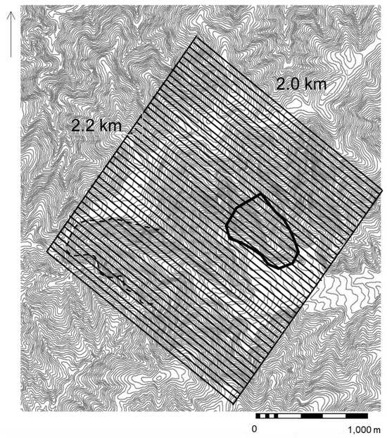
Figure 2.
The coverage and scanning lines of HEM measurement. The bold black polygon shows the D-GREATEM survey area [34].
3. Data Acquisition and Processing Methods
In this study, two types of airborne resistivity observation methods were applied and the acquired data were compared: HEM data and D-GREATEM data.
3.1. Drone-Grounded Electrical-Source Airborne Transient ElectroMagnetic (D-GREATEM) Survey
The UAV survey was conducted along eight lines (from Line A to Line H) across the study area at a flight speed of 10–13 km/h (Figure 3a). The survey period was 3–6 June 2020, and there was no precipitation during the two days prior to the survey period and during the survey period itself. The source signal was a time-varying current of 5.3 A transmitted to the subsurface by a 1 km long grounded electrical dipole source set parallel to the forest management road (Figure 3a). Steel electrodes were implanted in the ground to a depth of 0.3–0.4 m, with 30–50 electrodes 15 mm in diameter and 0.6 m in length on each side of the transmitter cable (Figure 3b). The electrode space is approximately 900 m. The vertical component of the secondary magnetic field related to subsurface resistivity was recorded by a sensor towed by the drone. The receiver was carried by the drone and it was flown at a height of approximately 100 m above the ground (Figure 3c). Magnetic field responses were recorded when the grounded electric dipole source was turned on and off. The switching of the transmitter and receiver signals on and off was synchronized to the circuit of the 1 pulse per second (PPS) signal in the GPS receiver (Figure 3d).
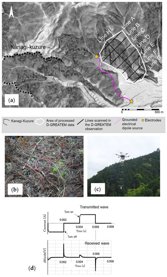
Figure 3.
Observation by D-GREATEM. (a) Setting and scanning lines of observation. (b) Photograph of the grounded electrical dipole source. (c) Photograph of the drone towing the transmitter. (d) Transmitted wave and received wave used in the measurement.
The waveforms were digitized through a 24-bit AD converter at a rate of 1 μs, and 8000 electromagnetic responses were recorded during one cycle of 8.0 ms (Figure 3d).
To use the magnetic field response data to estimate the resistivity, natural and artificial noise was removed by multiple stacking of the received signal at the ground monitoring site. The data stacking method was applied in each second. The data from 125 cycles were observed each second, and two transient signals, positive half cycles and negative reversed half cycles, were observed in one cycle. The positive half cycles and negative reversed half cycles were then stacked. Therefore, 250 records were stacked in each second. Moreover, the data were stacked every 10 m along the scanning lines.
After the noise removal operation, the inversion was performed by comparing the noise-free transient response curve of the vertical magnetic field with the theoretical response curve [30,35]. For the theoretical models, the height of the receiver recorded by GPS is used to estimate the vertical magnetic field. At deeper layers, the wavelength of propagating electromagnetic waves becomes longer. The closer to the surface, the higher the vertical resolution. Therefore, it is assumed that the vertical resolution of the surface layer is higher than that of deeper layers and the following thirteen horizontal layers from the surface to a depth of 200 m were set [35]: depths of 0.0–2.6 m, 2.6–7.7 m, 7.7–15.4 m, 15.4–25.6 m, 25.6–38.5 m, 38.5–53.8 m, 53.8–71.8 m, 71.8–92.3 m, 92.3–115.4 m, 115.4–141.0 m, 141.0–169.2 m, 169.2–200.0 m, and deeper than 200.0 m. By fitting the transient curve of the observation data to the theoretical model including the system response (Figure 4), the vertical structure of the resistivity was estimated by applying the 1D inversion assuming a horizontal layered structure model. To eliminate the error, data with RMSE > 0.20 was excluded. The resistivity was calculated from the surface to the depth at which the sensitivity was obtained.
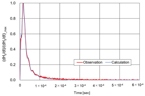
Figure 4.
Relative intensity to maximum amplitude of the transient curve including the system response derived from the field observation data and the modeling data. The RMSE of this data is 0.01.
3.2. Frequency-Domain Helicopter-Borne Electromagnetic (HEM) Survey
The frequency-domain helicopter-borne electromagnetic survey method was used. In this study, the same HEM resistivity data was used as in our previous research [34]. Here, we briefly explain the HEM survey and the acquired resistivity data.
HEM surveying determines the ground resistivity by measuring the intensity of a secondary magnetic field. Primary signals are generated by the flow of a sinusoidal current through transmitter coils to induce eddy currents in the subsurface layer. The lower the frequency of the transmitted electromagnetic waves, the deeper the ground penetration [36]. In order to estimate the resistivity up to a few hundred meters, these sensors were selected. The depth of the wave propagation is according to the frequency. Therefore, we used the HEM system employing transmitting and receiving coils oriented horizontally with frequencies of 140 kHz, 31 kHz, 6.9 kHz, 1.5 kHz, and 340 Hz. These coils were enclosed in a cylindrical container that was suspended by wires 30 m below a helicopter and flown at a height of ~35 m above the surface. The survey was conducted over 2.2 km × 2.0 km and the interval of the flight lines was approximately 50 m (Figure 2).
For the secondary field data, the in-phase and quadrature components at specific frequencies were measured. Due to the induction process within the subsurface layer, there is a small phase shift between the primary and secondary fields. The HEM resistivity was estimated by using phasor diagram for each frequency. With the measurement settings (the sensor height is approximately 30 m), the order of the in-phase and quadrature component measurement (102) is larger than system noise (100). Therefore, the signal to noise ratio was confirmed to be reasonable. After applying the spike noise removing and EM zero leveling operations to the secondary field data, an AEM data inversion homogeneous half-space model was derived from the relationship among in-phase, quadrature, and resistivity at a specific depth [37]. In order to exclude the influence of the upper layers from the deeper subsurface resistivity data, a differential method developed by Huang and Fraser [36] was applied to estimate the resistivity of each frequency, and residual leveling error was removed by using the 2D filter. Figure 5 shows the profile of the centroid depth and the corrected resistivity for each horizontal coil along Line A in Figure 3a. By assuming a horizontal-layered structure, the vertical structure of the resistivity was estimated [38].
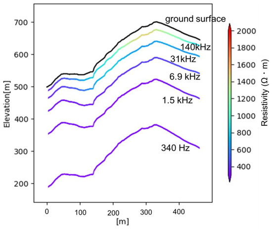
Figure 5.
Profile of the centroid depth of HEM observations and the corrected resistivity for the five horizontal coils with different frequencies along Line A in Figure 3a.
In order to compare the resistivity acquired by D-GREATEM and HEM, HEM resistivity data were extracted along the eight D-GREATEM flight lines (Figure 6). Moreover, the resistivity data were horizontally interpolated by the Kriging method and processed into 10 m resolution data at each frequency. In this study, the 140 kHz of HEM resistivity data (Figure 7b) was used to estimate the threshold of the HEM resistivity in the conductive zones.
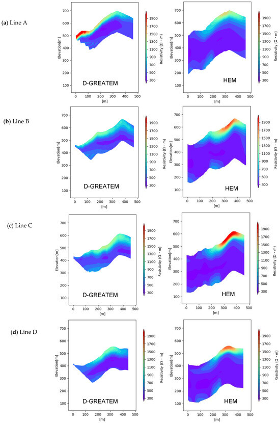
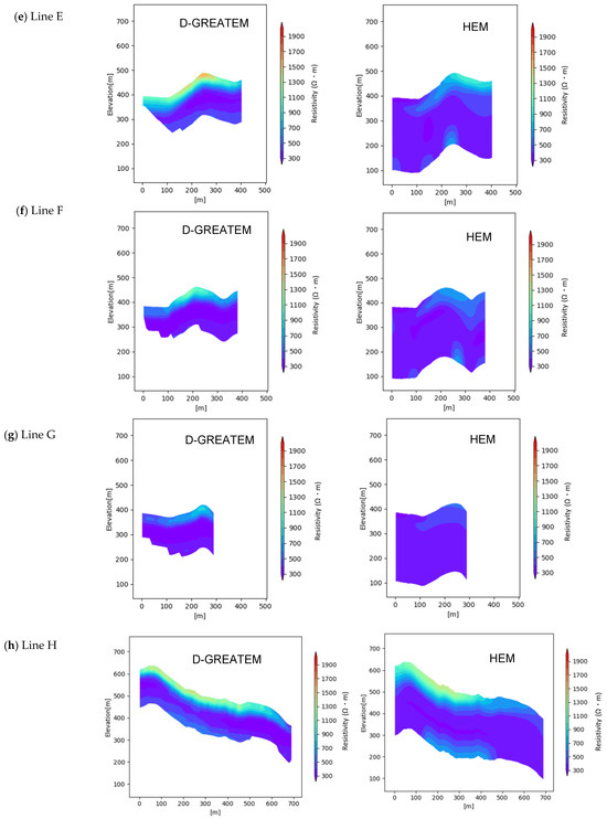
Figure 6.
Cross-sectional views of the resistivity of HEM and D-GREATEM along the eight flight lines. (a) Line A, (b) Line B, (c) Line C, (d) Line D, (e) Line E, (f) Line F, (g) Line G, (h) Line H.
Figure 7.
(a) Extracted valley floor using digital elevation data outlined in red. (b) HEM resistivity obtained at 140 kHz.
4. Results
4.1. Cross-Sectional View of the HEM and D-GREATEM Resistivity
In this section, we compare the resistivity obtained from the HEM and D-GREATEM observation methods. Rather than comparing the resistivity values one-to-one, we compare the resistivity distributions obtained via the HEM and D-GREATEM methods.
Figure 6 compares cross-sectional views of the resistivity of HEM and D-GREATEM along the eight flight lines. In this study, the near-surface zones from the ground surface to an approximately 100 m depth are focused on because they are closely related to landslide disasters. The HEM method has deeper exploration depths and greater resistivity contrast than the D-GREATEM method does, but the relative distributions of resistivity values are largely similar in the near-surface layer; both the HEM and D-GREATEM data reveal that the resistivity is higher around the ridge and the higher-resistivity zones are vertically distributed from the surface to depths of approximately 30–50 m.
However, the vertical pattern of the resistivity distribution differs between D-GREATEM and HEM measurements in some sections along Line A, Line B, and Line E, where HEM resistivity is low from the surface to deeper zones while, on the other hand, the D-GREATEM resistivity is high in the surface zones (depth 30 to 50 m) and low below the surface zones (Figure 6a,b,e). In the next section, the differences in resistivity obtained by D-GREATEM and HEM are investigated.
4.2. Comparison Between the HEM and D-GREATEM Resistivity
In some sections along Line A, Line B, and Line E, the resistivity of the vertical profile is different between D-GREATEM HEM. The resistivity of D-GREATEM is higher near the surface and it decreases with depth (Figure 6). On the other hand, the resistivity of HEM is low from the surface to a depth of 100 m, namely, the conductive zones are identified from the surface to a depth of 100 m. This difference probably shows the difference in vertical resolution between HEM and D-GREATEM in near-surface layers. This difference will be discussed in more detail in the following.
In order to analyze the difference in the estimated resistivity from HEM and D-GREATEM measurements, zones with different vertical profiles of resistivity distribution needed to be identified. In the previous study [34], it is shown that HEM resistivity obtained at 140 kHz is lower in the valley floor and sedimentary basins along the Sakihama River. This is consistent with the valley floor being saturated with groundwater and highly conductive. To determine the threshold of HEM resistivity in highly conductive zones, firstly, the valley floor was extracted as an area where the gradient of the slopes was smaller than 30° and the elevation lower than that of the surrounding area, which are delineated with red lines (Figure 7a). In the next step, by calculating the outliers of resistivity sampled within the valley floor (Figure 7b), the threshold of resistivity was defined. Since the HEM resistivity in the valley floor has a non-normal distribution, the robust Z score is calculated via the median (μ), first quantile (Q1), third quantile (Q3), and normalized interquartile range (NIQR) [39]. The Z score shows a standard normal distribution with a mean of 0 and a standard deviation of 1, and it shows a statistical measure of how many standard deviations a given data point is from the mean of a distribution.
x: measurement data, μ: median, Q1: the first quantile, Q3: the third quantile.
Z score = (x−μ)/NIQR
NIQR = (Q3−Q1)/(F(0.75)−F(0.25))
In this study, the threshold was set to Z score = 3 to exclude the 99th percentile. NIQR is calculated by using Q3, Q1, and the probability distribution function (F) as a normalized interquartile range of 0.75 and 0.25 (F(0.75)−F(0.25)): Q1 = 185.6 Ωm, Q3 = 298.0 Ωm, μ = 230.6 Ωm, and NIQR = (298.0−185.6)/1.3489 = 83.3. The resistivity value corresponding to Z score = 3 is 480.6 Ωm, which is nearly 500 Ωm. Thus, the threshold value for the highly conductive zone is set to 500 Ωm, and the areas where the resistivity is less than 500 Ωm are defined as the resistivity in the high-conductivity zone, namely, low resistivity.
In the cross-sections along A0–A1, B0–B1, and the E0–E1 (Figure 8), the zones with HEM resistivity lower than 500 Ωm are distributed both in layers from the surface to depths of approximately 30 m (surface layers) and below the surface layer (deeper layers), whereas the D-GREATEM resistivity is higher in the surface layers than in the deeper layers.
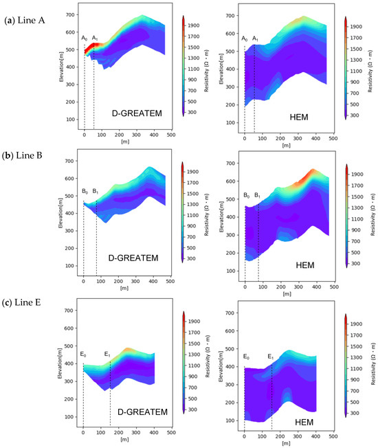
Figure 8.
Comparison of resistivity cross-sections showing differences between HEM and D-GREATEM observations. (a) Line A, (b) Line B, (c) Line E.
In Section 4.3, the differences between the HEM and D-GREATEM methods are discussed in terms of resistivity cross-section diagrams and outcrops and other field observation data.
4.3. The Comparative Analysis of D-GREATEM and HEM Resistivity with Outcrop Observations
Outcrop surveys were conducted at sites where different trends were identified between the HEM and D-GREATEM resistivity cross-sections along A0–A1 and B0–B1, respectively (Figure 9a). Point A0 is located on the ridge. At point A2, which is located in the vicinity of A0, the outcrop consists of alternating layers of sandstone and shale beds (N60E), and the rock masses are intensely fractured, dipping south by 14° (Figure 9b). The ridge is flanked by two drainage channels. In both channels (V1 and V2), erosion control weirs were constructed, and some spring water was discharged through drainage pipes (Figure 9c). These observations indicate that the surface layers are fractured and loosened and deeper layers are likely to be influenced by groundwater. This implies that the conductivity is low in the upper layers and the conductivity is high in the deeper layers.
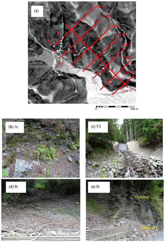
Figure 9.
Photographs of field observations: (a) Location of the survey points and flight lines, (b) outcrop at point A2, (c) channel V2, (d) slope at point B1, (e) outcrop and colluvium at point B1.
At point B1, the outcrop consists of alternating sandstone and shale beds (N60W), and the rock masses are intensely fractured and dip north by 28°N (Figure 9d). At point B1, the surface of the slope is covered with colluvium, probably because slope failures repeatedly occurred (Figure 9e). B0–B1 cross a drainage channel, where the V2 and V1 drainage channels meet. Therefore, zones along B0–B1 are affected by groundwater in the deeper zone. These observations indicate that the rock mass in the surface layer is loosened and the rock mass in the deeper layers is likely to be influenced by groundwater. This also implies that the conductivity is low in the upper layers and the conductivity is high in the deeper layers.
The observed features in the field surveys are compared with cross-sections of the resistivity from the HEM and D-GREATEM measurements. In the cross-sections along A0–A1 and B0–B1, the HEM resistivity values are similarly low (resistivity < 500 Ω m) both in the layer from the surface to an approximately 30 m depth (upper layers) and below the surface layer (the deeper layers), whereas the D-GREATEM resistivity values are higher in the surface layer than in the deeper layers. The D-GREATEM resistivity data reveal both zones: a zone in which the rock mass is loosened and unsaturated above the groundwater table, and a zone that is located below the groundwater table and saturated. The vertical resolution of HEM is according to the centroid depth of the measurement with each sensor, while the vertical resolution of D-GREATEM measurement is according to the assumed layers by the theoretical model. By estimating the resistivity in the same slopes with different methods, the characteristic of the measurement can be clearly shown. The details of the difference are discussed in Section 5.
5. Discussion
In this study, the resistivities obtained from HEM and D-GREATEM are compared. The resistivities of HEM and D-GREATEM have largely similar distributions; however, there are some differences, especially in the near-surface layers. The cross-sections of HEM resistivity tended to have higher resistivity in the ridges and lower resistivity in the valleys, whereas the D-GREATEM cross-sections had higher resistivity at the surface and lower resistivity at depths of 30 m or deeper on the loosened slopes, even in the valleys. In order to analyze the cause of the difference in resistivity between HEM and D-GREATEM, the assumed layers of the D-GREATEM method and the centroid depth of HEM are compared in the next paragraph.
The differences between the D-GREATEM and HEM measurements are analyzed. The HEM measurements derive the resistivity by assuming that the horizontal layer is at a specific depth, which depends on the frequency of measurements and resistivity [38], and the vertical resolution of the resistivity distribution depends on the frequency of the system of measurement. On the other hand, in the D-GREATEM method, the vertical resolution of the resistivity distribution depends on the observed transient response and the assumed structure. Figure 10 shows the comparison of the centroid depth of the measurements of HEM resistivity and the assumed theoretical layers for analyzing the D-GREATEM data along Line A. While HEM measurements were obtained from only one depth to a depth of 40 m below the ground surface, resistivity measurements using D-GREATEM were obtained from five depths. Therefore, D-GREATEM is suitable for measuring resistivity to estimate the loosened rock mass near the surface. Since the depth of earthquake-induced landslides has been reported to range from the surface to 30 m [40,41], D-GREATEM measurements are useful for estimating the susceptibility to earthquake-induced landslides on specific slopes. The HEM method is suitable for broadly and deeply measuring resistivity.
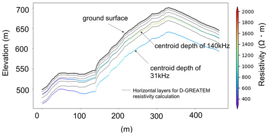
Figure 10.
Comparison of the centroid depth of measurements of HEM resistivity and the assumed horizontal layers for analyzing the D-GREATEM data along Line A.
It is important to select an appropriate observation method according to the observation target and purpose. Assuming that observations will be conducted, we compared two observation methods from multiple perspectives. HEM is suitable for wide-area surveys, while D-GREATEM is suitable for narrow-area surveys (Table 1).

Table 1.
Comparison of HEM and D-GREATEM for resistivity measurement (M.).
6. Conclusions
In this study, the use of drone-borne sensors for recording transient electromagnetic waves generated by a grounded electric dipole source was investigated to estimate the distribution of loosened rock masses in mountainous areas. A comparison was made between HEM and D-GREATEM methods. In particular, the vertical profiles of resistivity near the surface zones were different, and the D-GREATEM data revealed that it was possible to detect both loosened rock mass near the surface and rock mass saturated with groundwater beneath the surface layers. Therefore, D-GREATEM is suitable for intensive surveys of critical areas because it can capture near-surface loosened rock mass in detail and the drone is highly maneuverable. On the other hand, this method is not suitable for wide-area surveys because of its limited observation range. By combining methods such as HEM (for wide-area surveys) and D-GREATEM (for localized surveys), it is possible to conduct efficient surveys for estimating near-surface loosened rock mass zones in mountainous areas.
In mountainous regions, such as the Swiss Alps and the Himalayas, electrical resistivity tomography has been used to investigate the details of geological and hydrological structures in known landslides [42,43]. In order to widely detect unknown loosened rock mass zones in mountainous areas, combining HEM and D-GREATEM surveys should be useful.
Author Contributions
A.N. wrote the manuscript and interpreted the HEM and D-GREATEM data. S.H. supported the interpretation of the D-GREATEM data and the field work. A.J. (Akira Jomori), A.J. (Atsuyoshi Jomori), and T.T. performed the D-GREATEM measurements in this study area; M.O. performed the HEM resistivity data analysis; and H.H. supported the interpretation of the D-GREATEM data and the field work. H.O. supported the data visualization. Y.K. supported our research planning. All authors have read and agreed to the published version of the manuscript.
Funding
The D-GREATEM survey was funded by the SECOM Science and Technology Foundation. This research was part of a project funded by the KAKENHI (23K04348).
Data Availability Statement
The data that support the findings of this study are available from the corresponding author, Atsuko Nonomura, upon reasonable request.
Acknowledgments
This research was supported by Aki Forest Management Office.
Conflicts of Interest
Authors Akira Jomori, Tetsuya Toyama and Atsuyoshi Jomori are employed by the company NeoScience Co., Author Minoru Okumura is employed by the company Dia Nippon Engineering Consultants Co., Ltd., and Author Hiroaki Hoshino is employed by the company West Nippon Expressway Co., Ltd. The remaining authors declare that the research was conducted in the absence of any commercial or financial relationships that could be construed as a poten-tial conflict of interest.
Abbreviations
The following abbreviations are used in this manuscript:
| AEM | Airborne electromagnetic |
| D-GREATEM | Drone-grounded electrical-source airborne transient electromagnetic |
| EM | Electromagnetic |
| ERT | Electrical resistivity tomography |
| GREATEM | Grounded electrical-source airborne transient electromagnetic |
| HEM | Frequency-domain helicopter-borne electromagnetic |
| TEM | Transient electromagnetic |
References
- Xu, Q.; Fan, X.; Huang, R.; Westen, C. Landslide dams triggered by the Wenchuan Earthquake, Sichuan Province, south west China. Bull. Eng. Geol. Environ. 2009, 68, 373–386. [Google Scholar] [CrossRef]
- Lacroix, P. Landslides triggered by the Gorkha earthquake in the Langtang valley, volumes and initiation processes. Earth Planets Space 2016, 68, 46. [Google Scholar] [CrossRef]
- Doi, I.; Kamai, T.; Azuma, R.; Wang, G. A landslide induced by the 2016 Kumamoto Earthquake adjacent to tectonic displacement-Generation mechanism and long-term monitoring. Eng. Geol. 2019, 248, 80–88. [Google Scholar] [CrossRef]
- Chigira, M.; Tsou, C.; Matsushi, Y.; Hiraishi, N.; Matsuzawa, M. Topographic precursors and geological structures of deep-seated catastrophic landslides caused by Typhoon Talas. Geomorphology 2013, 201, 479–493. [Google Scholar] [CrossRef]
- Guzzetti, F.; Mondini, A.; Cardinali, M.; Fiorucci, F.; Santangelo, M.; Chang, K. Landslide inventory maps: New tools for an old problem. Earth-Sci. Rev. 2012, 112, 42–66. [Google Scholar] [CrossRef]
- Chang, K.; Chan, Y.; Chen, R.; Hsieh, Y. Geomorphological evolution of landslides near an active normal fault in northern Taiwan, as revealed by lidar and unmanned aircraft system data. Nat. Hazards Earth Syst. Sci. 2018, 18, 709–727. [Google Scholar] [CrossRef]
- Fan, X.; Zhan, W.; Dong, X.; Westen, C.; Xu, Q.; Dai, L.; Yang, Q.; Huang, R.; Havenith, H. Analyzing successive landslide dam formation by different triggering mechanisms: The case of the Tangjiawan landslide, Sichuan. Chin. Eng. Geol. 2018, 243, 128–144. [Google Scholar] [CrossRef]
- Chigira, M.; Kiho, K. Deep-seated rockslide-avalanches preceded by mass rock creep of sedimentary rocks in the Akaishi Mountains, central Japan. Eng. Geol. 1994, 38, 221–230. [Google Scholar] [CrossRef]
- Chigira, M.; Yagi, H. Geological and geomorphological characteristics of landslides triggered by the 2004 Mid Niigta prefecture earthquake in Japan. Eng. Geol. 2006, 82, 202–221. [Google Scholar] [CrossRef]
- Sato, H.; Hasegawa, H.; Fujiwara, S.; Tobita, M.; Koarai, M.; Une, H.; Iwahashi, J. Interpretation of landslide distribution triggered by the 2005 Northern Pakistan earthquake using SPOT5 imagery. Landslides 2007, 4, 113–122. [Google Scholar] [CrossRef]
- Chigira, M.; Wu, X.; Inokuchi, T.; Wang, G. Landslides induced by the 2008 Wenchuan earthquake, Sichuan, China. Geomorphology 2010, 118, 225–238. [Google Scholar] [CrossRef]
- Godio, A.; Bottino, G. Electrical and electromagnetic investigation for landslide characterization. Phys. Chem. Earth Part C Sol. Terr. Planet. Sci. 2001, 26, 705–710. [Google Scholar]
- Lapenna, V.; Lorenzo, P.; Perrone, A.; Piscitelli, S.; Sdao, F.; Rizzo, E. High-resolution geoelectrical tomographies in the study of Giarrossa landslide (southern Italy). Bull. Eng. Geol. Environ. 2003, 62, 259–268. [Google Scholar] [CrossRef]
- Schrott, L.; Sass, O. Application of field geophysics in geomorphology: Advances and limitations exemplified by case studies. Geomorphology 2008, 93, 55–73. [Google Scholar] [CrossRef]
- Kasprzak, M.; Jancewicz, K.; Różycka, M.; Kotwicka, W.; Migoń, P. Geomorphology- and geophysics-based recognition of stages of deep-seated slope deformation (Sudetes, SW Poland). Eng. Geol. 2019, 260, 105230. [Google Scholar] [CrossRef]
- Perrone, A.; Lapenna, V.; Piscitelli, S. Electrical resistivity tomography technique for landslide investigation: A review. Earth-Sci. Rev. 2014, 135, 65–82. [Google Scholar] [CrossRef]
- Rønning, J.S.; Ganerød, G.V.; Fabienne, E.D.; Reiser, F. Resistivity mapping as a tool for identification and characterisation of weakness zones in crystalline bedrock: Definition and testing of an interpretational model. Bull. Eng. Geol. Environ. 2014, 73, 1225–1244. [Google Scholar] [CrossRef]
- Hen-Jones, R.M.; Hughes, P.N.; Stirling, R.A.; Glendinning, S.; Chambers, J.E.; Gunn, D.A.; Cui, Y.J. Seasonal effects on geophysical–geotechnical relationships and their implications for electrical resistivity tomography monitoring of slopes. Acta Geotech. 2017, 12, 1159–1173. [Google Scholar] [CrossRef]
- Palacky, G. Resistivity characteristics of geologic targets. In Electromagnetic Methods in Applied Geophysics, Investigations in Geophysics No. 3; Nabighian, M., Ed.; Society of Exploration Geophysicists: Houston, TX, USA, 1988; pp. 53–129. [Google Scholar]
- Nakazato, H.; Konishi, N. Subsurface structure exploration of wide landslide area by Aerial electromagnetic exploration. Landslides 2005, 2, 165–169. [Google Scholar] [CrossRef]
- Baranwal, V.; Brönner, M.; Rønning, J.; Elvebakk, H.; Dalsegg, E. 3D interpretation of helicopter-borne frequency-domain electromagnetic (HEM) data from Ramså Basin and adjacent areas at Andøya, Norway. Earth Planets Space 2020, 72, 52. [Google Scholar] [CrossRef]
- Høyer, A.; Jørgensen, F.; Foged, N.; He, X.; Christiansen, A. Three-dimensional geological modelling of AEM resistivity data –A comparison of three methods. J. Appl. Geophys. 2015, 115, 65–78. [Google Scholar] [CrossRef]
- Auken, E.; Christiansen, A.; Westergaard, J.; Kirkegaard, C.; Foged, N.; Viezzoli, A. An integrated processing scheme for high-resolution airborne electromagnetic surveys, the SkyTEM system. Explor. Geophys. 2009, 40, 184–192. [Google Scholar] [CrossRef]
- Steuer, A.; Siemon, B.; Auken, E. A comparison of helicopter-borne electromagnetics in frequency- and time-domain at the Cuxhaven valley in Northern Germany. J. Appl. Geophys. 2009, 67, 194–205. [Google Scholar] [CrossRef]
- Mogi, T.; Kusunoki, K.; Kaieda, H.; Ito, H.; Jomori, A.; Jomori, N.; Yuuki, Y. Grounded electrical-source airborne transient electromagnetic (GREATEM) survey of Mount Bandai, north-eastern Japan. Explor. Geophys. 2009, 40, 1–7. [Google Scholar] [CrossRef]
- Okazaki, K.; Mogi, T.; Utsugi, M.; Ito, Y.; Kunishima, H.; Yamazaki, T.; Takahashi, Y.; Hashimoto, T.; Ymamaya, Y.; Ito, H.; et al. Airborne electromagnetic and magnetic surveys for long tunnel construction design. Phys. Chem. Earth (A,B,C) 2011, 36, 1237–1246. [Google Scholar] [CrossRef]
- Ito, H.; Kaieda, H.; Mogi, T.; Jomori, A.; Yuuki, Y. Grounded electrical-source airborne transient electromagnetics (GREATEM) survey of Aso Volcano, Japan. Explor. Geophys. 2014, 45, 43–48. [Google Scholar] [CrossRef]
- Allah, S.; Mogi, T.; Ito, H.; Jymori, A.; Yuuki, Y.; Fomenko, E.; Kiho, K.; Kaieda, H.; Suzuki, K.; Tsukuda, K. Three-dimensional resistivity modelling of grounded electrical-source airborne transient electromagnetic ((GREATEM) survey data from the Nojima Fault, Awaji Island, south-east Japan. Explor. Geophys. 2014, 45, 49–61. [Google Scholar] [CrossRef]
- Allah, S.; Mogi, T. Three-dimensional resistivity modeling of GREATEM survey data from Ontake Volcano, northwest Japan. Earth Planets Space 2016, 68, 76. [Google Scholar] [CrossRef]
- Jomori, A.; Jomori, N.; Jomori, A.; Kondo, T.; Yuuki, Y.; Shinsei, A. Development of airborne transient electromagnetics system using Drone: D-GREATEM, D-TEM [GLS], D-TEM [ALS]. BUTSURI-TANSA (Geopysical Explor.) 2020, 73, 83–95. (In Japanese) [Google Scholar] [CrossRef]
- Parshin, A.; Bashkeev, A.; Davidenko, Y.; Persova, M.; Iakovlev, S.; Bukhalov, S.; Grebenkin, N.; Tokareva, M. Lightweight Unmanned Aerial System for Time-Domain Electromagnetic Prospecting-The Next Stage in Applied UAV-Geophysics. Appl. Sci. 2021, 11, 2060. [Google Scholar] [CrossRef]
- Chigira, M. Geological prediction of rock avalanches. In Proceedings of the 8th International Congress of the International Association of Engineering Geology and Environment, Vancouver, BC, Canada, 21–25 September 1998; pp. 1409–1414. [Google Scholar]
- Nonomura, A.; Hasegawa, S. Regional extraction of flexural-toppled slopes in epicentral regions of subduction earthquakes along the Nankai Trough using DEMs. Environ. Earth Sci. 2013, 68, 139–149. [Google Scholar] [CrossRef]
- Nonomura, A.; Hasegawa, S.; Kageura, R.; Kawato, K.; Chiba, T.; Onoda, S.; Dahal, R. A method for regionally mapping gravitationally deformed and loosened slopes using helicopter-borne electromagnetic resistivity data. Nat. Hazards 2016, 81, 123–144. [Google Scholar] [CrossRef]
- Ward, S.; Hohmann, G. Electromagnetic theory for geophysical applications. In Electromagnetic Methods in Applied Geophysics; Nabighian, M.N., Ed.; SEG: Tulsa, OK, USA, 1988; pp. 131–311. [Google Scholar]
- Huang, H.; Fraser, D.C. The differential parameter method for multifrequency airborne resistivity mapping. Geophysics 1996, 61, 100–109. [Google Scholar] [CrossRef]
- Sinha, A.K.; Collett, L.S. Electromagnetic Fields of Oscillating Magnetic Dipoles Placed over a Multilayer Conducting Earth; Geological Survey of Canada Paper; Department of Energy, Mines and Resources: Ottawa, ON, Canada, 1973; Volume 73, pp. 1–48. [Google Scholar]
- Siemon, B. Electromagnetic methods–frequency domain. In Groundwater Geophysics; Kirsch, R., Ed.; Springer: Berlin/Heidelberg, Germany, 2009; pp. 155–178. [Google Scholar]
- Ishibashi, Y.; Asada, S.; Igaki, H.; Yamada, S.; Tsuruta, S.; Shimura, M.; Kakita, K.; Ono, A.; Sakata, M. Results of proficiency testing for determination of Dioxins in marine sediment (3rd round) based on ISO/IEC Guide 43-1. BUNSEKI KAGAKU 2005, 54, 235–242. [Google Scholar] [CrossRef][Green Version]
- Yunus, A.; Xinyu, C.; Catani, F.; Subramaniam, S.; Fan, X.; Jie, D.; Sajinjumar, K.; Gupta, A.; Avtar, R. Earthquake-induced soil landslides: Volume estimates and uncertainties with the existing scaling exponents. Sci. Rep. 2023, 13, 8151. [Google Scholar] [CrossRef] [PubMed]
- Saito, H.; Uchiyama, S.; Hayakawa, Y.; Obanawa, H. Landslides triggered by an earthquake and heavy rainfalls at Aso volcano, Japan, detected by UAS and SfM-MVS photogrammetry. Prog. Earth Planet. Sci. 2018, 5, 15. [Google Scholar] [CrossRef]
- Biévre, G.; Jongmans, D.; Lebourg, T.; Carriére, S. Electrical resistivity monitoring of an earthslide with electrodes located outside the unstable zone (Pont-Bourquin landlide, Swiss Alps). Near Surf. Geophys. 2021, 19, 225–239. [Google Scholar] [CrossRef]
- Singh, S.; Gautam, P.; Bagchi, D.; Singh, S.; Kumar, S.; Kannaujiya, S. 2D Electrical resistivity imaging for geothermal groundwater characterization and rejuvenation of the Gaurikund hot spring in the Main Central Thrust (MCT) zone of the Garhwal Himalaya, Uttrakhand, India. Groundw. Sustain. Dev. 2021, 15, 100686. [Google Scholar] [CrossRef]


Disclaimer/Publisher’s Note: The statements, opinions and data contained in all publications are solely those of the individual author(s) and contributor(s) and not of MDPI and/or the editor(s). MDPI and/or the editor(s) disclaim responsibility for any injury to people or property resulting from any ideas, methods, instructions or products referred to in the content. |
© 2025 by the authors. Licensee MDPI, Basel, Switzerland. This article is an open access article distributed under the terms and conditions of the Creative Commons Attribution (CC BY) license (https://creativecommons.org/licenses/by/4.0/).